Literature Study

The transcritical organic Rankine cycle

Department of Flow, Heat and Combustion Mechanics

Catternan Tom

Table of ContentTable of Content.....................................................................................................................................2

Nomenclature........................................................................................................................................6

Chapter 1 Introduction...........................................................................................................................8

Chapter 2 The organic Rankine cycle...................................................................................................10

1. Introduction..........................................................................................................................10

2. Components.........................................................................................................................12

3. Applications of organic Rankine cycles.................................................................................13

2.1 Biomass [10].................................................................................................................13

2.2 Geothermal heat sources [10]......................................................................................14

2.3 Solar energy [20]...........................................................................................................15

2.4 Waste heat recovery from internal combustion engines [10]......................................16

2.5 Industrial waste heat [22].............................................................................................17

2.5.1 Cement industry...................................................................................................17

2.5.2 Steel industry........................................................................................................18

2.5.3 Glass industry........................................................................................................18

Chapter 3 Transcritical organic Rankine cycle.....................................................................................19

1. Introduction..........................................................................................................................19

2. Temperature profile in the heat exchanger..........................................................................22

3. The transcritical cycle...........................................................................................................23

Chapter 4 Classification of working fluids-Selection criteria................................................................26

1. Introduction..........................................................................................................................26

2. Classification and selection criteria of working fluids...........................................................27

2.1 Screening criteria..........................................................................................................27

2.1.1 Safety criterion (ASHRAE 34)................................................................................27

2.1.2 Environmental criterion........................................................................................28

2.1.3 Stability of the working fluid and compatibility with materials in contact............30

2.1.4 Thermophysical properties...................................................................................30

2.1.4.1 Type of fluids.....................................................................................................30

2.1.4.1.1 Trans – and subcritical ‘wet’ cycles.............................................................32

2.1.4.1.2 Trans – and subcritical ‘dry’ cycles..............................................................33

2.1.4.2 Influence of latent heat, density and specific heat............................................35

2.1.4.3 Critical temperature and pressure.....................................................................35

2.1.4.4 Mixtures.............................................................................................................36

2.1.5 Availability and cost of working fluids...................................................................37

2.2 Cycle criteria - Selection by performance indicator......................................................38

2.2.1 Thermodynamic performance indicators..............................................................38

2.2.1.1 First law efficiency - Thermal efficiency of the cycle – Net power output.........38

2.2.1.2 Second law efficiency - Exergy efficiency...........................................................39

2.2.1.2.1 System total irreversibility..........................................................................43

2.2.1.2.2 Exergy destruction factor (EDF)..................................................................45

2.2.1.3 Other efficiencies...............................................................................................45

2.2.1.3.1 Heat-exchanger and system efficiency [10] [23].........................................45

2.2.1.3.2 Recovery efficiency [65]..............................................................................46

2.2.1.3.3 Rankine cycle efficiency (bron)...................................................................46

2.2.2 Heat exchanger performance indicators...............................................................47

2.2.2.1 Heat transfer capacity UA capacity....................................................................47

2.2.2.2 Total heat exchanger surface.............................................................................47

2.2.2.3 Heat exchanger efficiency..................................................................................48

2.2.3 Cost performance indicators.................................................................................49

2.2.3.1 APR....................................................................................................................49

2.2.3.2 Levelized energy cost LEC..................................................................................49

3. Working fluids for organic Rankine cycles............................................................................51

3.1 Fluid candidates............................................................................................................51

3.1.1 Group 1: Fluids ammonia, benzene and toluene..................................................53

3.1.2 Group 2: Fluids R170, R744, R41, R23, R116, R32, R125 and R143a.....................54

3.1.3 Group 3: Fluids propyne, HC270, R152a, R22 and R1270.....................................54

3.1.4 Group 4: Fluids R21, R142b, R134a, R290, R141b, R123, R245ca, R245fa, R236ea, R124, R227ea, R218..............................................................................................................54

3.1.5 Group 5: Fluids R601, R600, R600a, FC-4-1-12, RC318, R-3-1-10.........................54

3.2 Working fluids for transcritical organic Rankine cycles.................................................55

Chapter 5 Modelling.............................................................................................................................58

1. Introduction..........................................................................................................................58

2. Energy balances....................................................................................................................58

3.3 Pump............................................................................................................................59

3.4 Vapour generator.........................................................................................................59

3.5 Expander.......................................................................................................................59

3.6 Condenser.....................................................................................................................59

3.7 Regenerator (Internal Heat Exchanger)........................................................................60

3. Heat transfer........................................................................................................................61

3.1 Vapour generator.........................................................................................................62

3.1.1 Working fluid – heat transfer coefficient..............................................................62

3.1.2 Heat source...........................................................................................................63

3.2 Condenser.....................................................................................................................63

3.2.1 Working fluid........................................................................................................64

3.2.1.1 Single-phase heat transfer coefficient...............................................................64

3.2.1.2 Two-phase heat transfer coefficient..................................................................64

3.2.2 Cooling fluid..........................................................................................................65

3.3 Evaporator (subcritical).................................................................................................65

3.3.1 Working fluid single-phase heat transfer coefficient............................................65

3.3.2 Working fluid two-phase heat transfer coefficient...............................................65

4. Pressure drop.......................................................................................................................66

4.1 Vapour generator.........................................................................................................66

4.1.1 Working fluid........................................................................................................66

4.2 Condenser.....................................................................................................................66

4.2.1 Working fluid........................................................................................................66

4.2.1.1 Single-phase pressure drop...............................................................................66

4.2.1.2 Two-phase pressure drop..................................................................................66

4.2.2 Cooling fluid - single-phase pressure drop............................................................66

4.3 Evaporator (subcritical).................................................................................................67

4.3.1.1 Single-phase pressure drop...............................................................................67

4.3.1.2 Two-phase pressure drop..................................................................................67

Chapter 6 Fluid selection and cycle optimization.................................................................................68

1. Parametric study and cycle optimization..............................................................................68

2.1 Energy analysis.............................................................................................................70

2.2 Exergy analysis..............................................................................................................73

2.3 Recovery efficiency.......................................................................................................77

2.4 Total heat transfer capacity UA....................................................................................78

2.5 Heat exchanger surface................................................................................................79

2.6 Thermo-economic analysis...........................................................................................81

2. Fluid selection.......................................................................................................................85

Chapter 7 Heat exchanger design.........................................................................................................86

Chapter 8 Experimental organic Rankine cycle....................................................................................87

References............................................................................................................................................90

NomenclatureH Enthalpy (kJ)

h Specific enthalpy (kJ/kg)

m Mass (kg)

m Mass flow rate (kg/s)

P Power (kW)

Q Heat (kJ)

q Specific heat (kJ/kg)

Q Heat flow rate (kJ/s)

T Temperature (°C)

S Entropy (kJ/K)

s Specific entropy (kJ/kgK)

W Work (kJ)

w Specific work (kJ/kg)

Greek symbols

η Efficiency (%)

ηth Thermal efficiency (%)

ηt Total heat-recovery efficiency (%)

Φ Heat availability (-)

Sub- and superscripts

s Isentropic

crit Critical

CS Cold Source

Mech Mechanical

WH Waste heat

Evap Evaporator

Exp Expander

Cond Condenser

Vap-gen Vapour Generator

WH Waste heat

In Inlet

Out Outlet

1,2,3… State points

Acronyms

ORC Organic Rankine Cycle

IHE Internal Heat Exchanger

Chapter 1IntroductionDuring the last 100 years, the world’s population and industrial activity increased considerably. As a consequence, the energy demand during this period has risen almost exponentially.

Fossil fuels have been used to achieve great technological and economic progress. However, the increasing consumption of these limited resources has led to more and more environmental problems such as global warming, ozone depletion and atmospheric pollution. Furthermore, along with the fast development of industry, energy shortages and blackouts have appeared more and more frequently all over the world.

This situation illustrates the necessity of developing new clean energy sources and also the necessity of decreasing the energy intensity in all sectors of the economy.

There is much effort in using renewable energy sources like solar, water and wind energy. But also biomass and the utilization of low-grade heat sources, such as geothermal resources, exhaust gas of gas turbines and waste heat from industrial plants can be used for the production of electricity. These resources have potential in reducing consumption of fossil fuels and in relaxing environmental problems.

The valorisation of industrial thermal wastes seems to offer an important potential. As an example, 71% of the 3,220 PJ annually consumed by the eight principal industrial sectors in Canada are thrown away in the form of thermal wastes and represent an annual recovery potential of 2,280 PJ of thermal energy [1].

Experts assume that the annual unused industrial waste heat potential amounts to 140TWh in Europe alone, implying a CO2-reduction potential of about 14Mton of CO2 per annum [2]. In Flanders alone, several studies indicate the enormous amount (order of several hundreds of MWth) of available thermal power at low temperatures (± 100°). Such ‘waste’ heat is available in the steel, cement, glass, paper, plastic, chemical and food industry in the form of cooling water, exhaust air of drying installations, flue gasses, afterburners, … [3]. In fact today only the first steps are being made to recover the energy present in the waste heat and the driving force for doing so is energy efficiency:

Rising energy prices force industry to make their processes more energy efficient from a purely economic point of view [4].

EU (and regional) legislation related to CO2-emission reductions (the 202020-goals) force industry to reduce their CO2-emissions in order to be compliant to the rules [EU17215/08].

The organic Rankine cycle (short: ORC) is a promising process for conversion of low and medium temperature heat to electricity. Hence, ORC technology has a big economical potential and can help to realize the 202020 goals. However, there are only few applications that can use this energy directly as heat. Furthermore, transportation of large quantities of heat over long distances is not

practical. In situ utilization of this heat as the source of a power cycle is thus a concept generating a lot of interest.

In chapter 2 an introduction about organic Rankine cycles and an overview of the main components are given. Further, the main applications of organic Rankine cycles are discussed.

In chapter 3 the transcritical Rankine cycle and its advantages are explained.

Chapter 4 gives an overview of the selection criteria for the working fluids and lists the potential candidates for transcritical Rankine cycles.

In chapter 5 the thermodynamic and heat exchanger models are described, which will be used in the numerical simulations with EES.

In chapter 6 an overview is given of parametric studies done by several researchers and the influence of the key parameters on different performance indicators are studied.

Chapter 7 describes the heat exchanger design and chapter 8 shows an existing experimental setup of a solar-powered Rankine cycle.

Chapter 2 The organic Rankine cycle

1. Introduction

The process of an organic Rankine cycle works like the traditional Clausius-Rankine steam power cycle, but instead of water it uses an organic working fluid.

Advantages presented by water as working fluid are [5]:

very good thermal/chemical stability (no risk of decomposition); very low viscosity (less pumping work required); good energy carrier (high latent and specific heat); non-toxic, non-flammable and no threat to the environment (zero ODP, zero GWP); cheap and abundant (present almost everywhere on earth).

However, many problems are encountered when using water as working fluid [6]:

need of superheating to prevent condensation during expansion; risk of erosion of turbine blades; excess pressure in the evaporator; complex and expensive turbines.

The traditional steam cycle does not give a satisfying performance when utilizing low-grade waste heat because of its low thermal efficiency and large volume flows (Hung et al. [7]). For low-temperature waste heat recovery in small to medium scale power plants, organic fluids have been proposed, because of its several advantages over conventional steam (Tchanche et al. [8]):

less heat is needed during the evaporation process; the evaporation process takes place at lower pressure and temperature; the expansion process ends in the vapour region and hence the superheating is not required

and the risk of blades erosion is avoided; the smaller temperature difference between evaporation and condensation also means that

the pressure drop/ratio will be much smaller and thus simple single stage turbines can be used.

In contrast to water, the expansion in the turbine ends for most organic fluids not in the wet steam regime but in the gas phase above condenser temperature. Thus, often an internal heat exchanger (or regenerator) is used to improve efficiency by preheating the liquid working fluid with the expanded superheated vapour before the condenser.

The difference between water and several organic fluids is shown in a T,s-diagram in Figure 1.

Figure 1: Comparison T,s-diagram of water and an organic fluid.

The diagram shows the saturation lines for water and a few organic fluids. It can be clearly seen, that the critical point (top of the saturation curve) of an organic fluid is reached at lower pressures and temperatures compared with water.

A comparison of the fluid properties between an organic fluid and steam is presented in Table 1 [8].

Table 1: Summary of fluid properties comparison in steam and organic Rankine cycles

A big challenge for optimizing an organic Rankine cycle for waste heat recovery is the choice of the proper organic working fluid and the design of the cycle for variable heat input and waste heat temperature.

A configuration and the cycle plotted in a T,s-diagram of an organic Rankine cycle is shown in Figure 2.

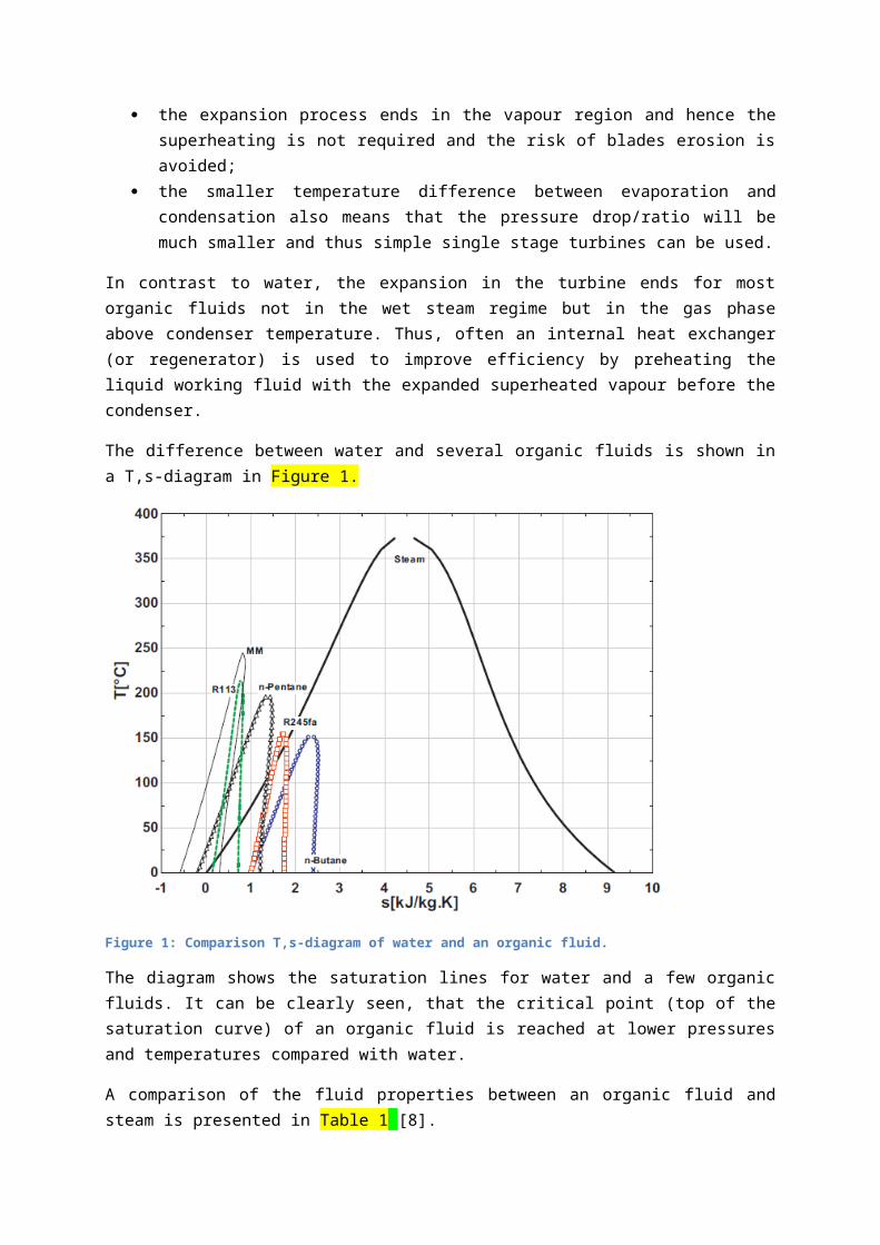
Figure 2: Demonstration of an organic Rankine cycle: (a) Configuration of an organic Rankine cycle; (b) An organic Rankine cycle process in T–s diagram.

2. Components

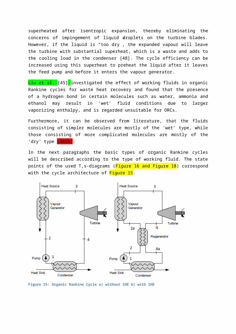
A general description of an organic Rankine cycle can be found in Figure 3. As can be seen, the cycle exists out of several components, which are similar to a normal cooling cycle. The main components are:

a feeding pump of the organic fluid; a vapour generator; a turbine or expander; a condenser; and if necessary an internal heat exchanger or regenerator.

Figure 3: Organic Rankine Cycle a) without IHE b) with IHE

An advantage of organic working fluids is that the turbine built for ORCs typically requires only a single-stage expander, which results in a simpler, more economical system in terms of capital costs and maintenance [9].

The power range of ORC process applications can vary from a few kW up to 1 MW. The most commonly used turbines which are available in the market cover a range above 50 kW. Therefore, expanders in the power range below 10 kW have to be found.

Schuster et al. gives a short overview of the used expanders in ORC technology in [10], as summarized below.

A very promising solution to this turbine market problem is to use the scroll expander. This expander works in a reverse way as the scroll compressor, which is a positive displacement machine used in air conditioning technologies. Scroll machines have two identical coils, one of which is fixed and the other is orbiting with 180° out of phase forming crescent-shaped chambers, whose volumes accelerate with increasing angle of rotation.

Another promising machine for the expansion of the working fluid is the screw type compressor. Rotary screw compressors are also positive displacement machines. The mechanism for gas compression utilizes either a single screw element or two counter rotating intermeshed helical screw elements housed within a specially shaped chamber. As the mechanism rotates, the meshing and rotation of the two helical rotors produces a series of volume-reducing cavities. Gas is drawn in through an inlet port in the casing, captured in a cavity, compressed as the cavity reduces in volume, and then discharged through another port in the casing. Screw type compressors can work in the reverse direction also as expanders providing similar efficiencies. The effectiveness of the screw mechanism is dependent on close fitting clearances between the helical rotors and the chamber for sealing of the compression cavities.

Recently, Gerotor and scroll expanders were experimentally tested for performance in organic Rankine cycles [11].

3. Applications of organic Rankine cycles

Organic Rankine cycles can be used with several (renewable) energy sources:

biomass; geothermal heat sources; waste heat recovery of internal combustion engines or industrial plants; solar energy.

2.1 Biomass [10]

Combustion is the most common process for energy production from this renewable fuel. The fact that it is CO2-free has lead the countries to the financial support of biomass combustion technologies.

Some countries, for example Germany, support extra the use of innovative technologies such as ORC process. Therefore, many examples of ORC powered Combined Heat and Power plants are working in central Europe like Stadtwärme Lienz Austria 1000 kWel, Sauerlach Bavaria 700 kWel, Toblach South Tyrol 1100 kWel, Fußach Austria 1500 kWel [12].

The main reason why the construction of new ORC plants increases is the fact that it is the only proven technology for decentralized applications for the production of power up to 1 MWel from solid fuels like biomass. The electrical efficiency of the ORC process lies between 6-17 % [13].

However, even if the efficiency of the ORC is low, it has advantages, like the fact that the system can work without maintenance, which leads to very low personnel costs. Furthermore the organic working fluid has, in comparison with water, a relatively low enthalpy difference between high pressure and expanded vapour. This leads to higher mass flows compared with water. The application of larger turbines due to the higher mass flow reduces the gap losses compared to a water-steam turbine with the same power. The efficiency of an organic Rankine cycle turbine is up to 85 % and it has an outstanding part load behavior [14].

The exhaust gas from biomass combustion has a temperature of about 1000 °C. For the use of the exhaust heat in the ORC process, the working fluid which is used in most of the biomass applications is octamethyltrisiloxane (OMTS). Drescher et al. [15] discusses the use of other organic fluids and calculated an efficiency rise of around three percentage points in the case where Butylbenzene (C10H14) is used.

For biomass applications, the temperature levels are significantly higher than low-grade heat applications (see Table 2 for typical temperatures of ORC for biomass application).

Table 2: Typical temperatures of ORC for biomass application

2.2 Geothermal heat sources [10]

Geothermal heat sources vary in temperature from 50 to 350°C, and can either be dry, mainly steam, a mixture of steam and water, or just liquid water. The temperature of the resource is a major determinant of the type of technologies required to extract the heat and the uses to which it can be applied [16] [17].

Generally, the high-temperature reservoirs are the ones most suitable for commercial production of electricity. Dry steam and flash steam systems are widely used to produce electricity from high-temperature resources. Dry steam systems use the steam from geothermal reservoirs as it comes from wells, and route it directly through turbine/generator units to produce electricity. Flash steam plants are the most common type of geothermal power generation plants in operation today. In flash

steam plants, hot water under very high pressure is suddenly released to a much lower pressure, allowing some of the water to convert into steam, which is then used to drive a turbine.

Medium-temperature geothermal resources, where temperatures are typically in the range of 100–220°C, are by far the most commonly available resource. Binary cycle power plants are the most common technology for utilizing such resources for electricity generation. There are many different technical variations of binary plants including the organic Rankine cycles. Binary cycle geothermal power generation plants differ from dry steam and flash steam systems in that the water or the steam from the geothermal reservoir never comes in contact with the turbine/generator units. In binary systems, the water from the geothermal reservoir is used to heat a secondary fluid which is vaporized and used to turn the turbine/generator units. The geothermal water and the working fluid are each confined in separate circulating systems and never come in contact with each other.

Although binary power plants are generally more expensive to build than steam-driven plants, they have several advantages. The working fluid boils and flashes to a vapour at a lower temperature than water does, so electricity can be generated from reservoirs with lower temperatures.

An example of a geothermal plant using the ORC process is the plant Neustadt-Glewe in Germany [18], which was the first geothermal power plant in Germany [19]. This plant is a simple organic Rankine cycle plant which uses n- Perfluorpentane (C5F12) as working fluid. It uses water of approximately 98°C located at a depth of 2,250 m and converts this heat to 210 kW electricity by means of an organic Rankine cycle (ORC) turbine. Another well-known geothermal plant using ORC process is the Altheim Rankine Cycle Turbogenerator in the upper Austrian city Altheim. This plant produces 1 MWel power and supply heat to a small district heating system. The thermal power input from the geothermal water is equal to 12.4 MWth.

2.3 Solar energy [20]

Concentrating solar power is a well-proven technology: the sun is tracked and reflected on a linear or on a punctual collector, transferring heat to a fluid at high temperature. The heat is then transferred to a power cycle generating electricity. The three main concentrating technologies are the parabolic dish, the solar tower, and the parabolic trough. Parabolic dishes and solar towers are punctual concentration technologies, leading to a higher concentration factor and to higher temperatures. The best suited power cycles for these technologies are the Stirling engine (small-scale plants), the steam cycle, or even the combined cycle, for solar towers.

Parabolic troughs work at a lower temperature (300°C to 400°C). Up to now, they were mainly coupled to traditional steam Rankine cycles for power generation (Müller-Steinhagen & Trieb, 2004). The same limitation as in geothermal or biomass power plants remains: steam cycles require high temperatures, high pressures, and therefore high installed power to be profitable.

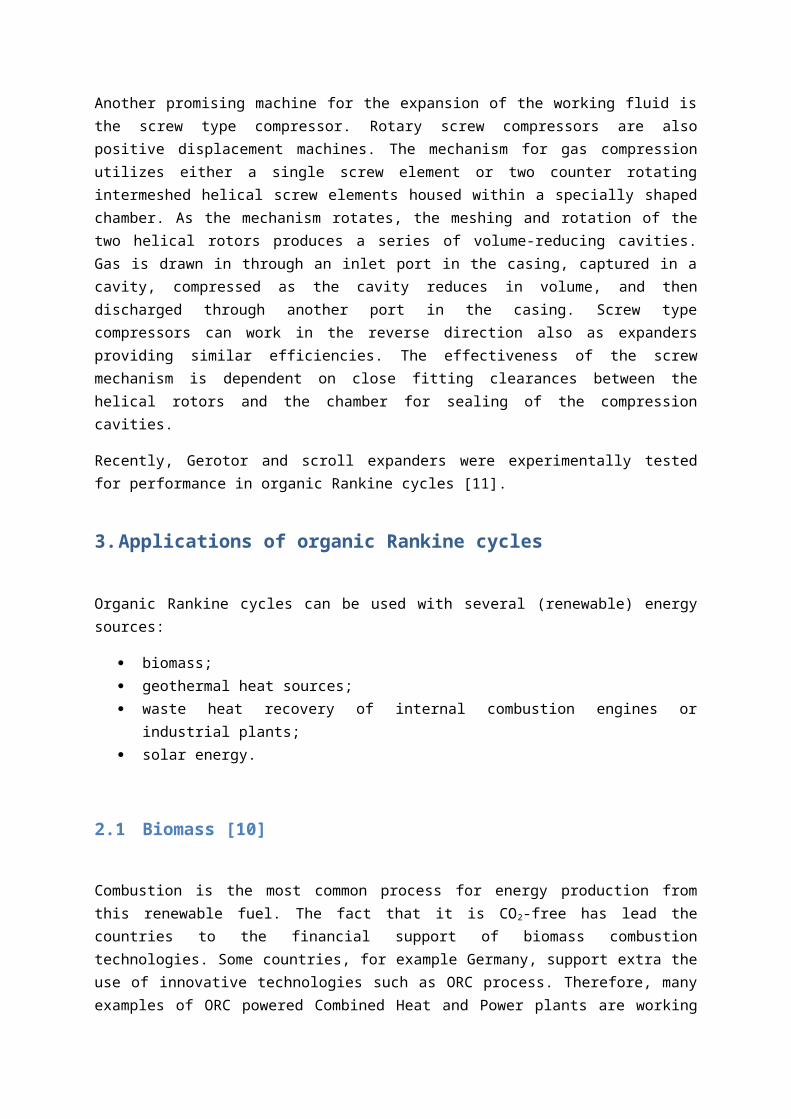
Organic Rankine cycles seem to be a promising technology to decrease investment costs at small scale: they can work at lower temperatures, and the total installed power can be reduced down to the kW scale. The working principle of solar energy powered Rankine cycle for combined heat recovery and power generation is presented in Figure 4. Technologies such as Fresnel linear

concentrators (Ford, 2008) are particularly suitable for solar ORCs since they require lower investment cost, but work at a lower temperature.

Up to now, very few CSP plants using ORC are available on the market:

A 1MWe concentrating solar power ORC plant was completed in 2006 in Arizona. The ORC module uses n-pentane as the working fluid and shows an efficiency of 20 %. The overall solar to electricity efficiency is 12.1% on the design point (Canada, 2004).

Some very small-scale systems are being studied for remote off-grid applications. The only available proof-of-concept is a 1 KWe system installed in Lesotho by “STG International” for rural electrification. The goal of this project is to develop and implement a small scale solar thermal technology utilizing medium temperature collectors and an ORC to achieve economics analogous to large-scale solar thermal installations. This configuration aims at replacing or supplementing Diesel generators in off-grid areas of developing countries, by generating clean power at a lower levelized cost.

Figure 4: Solar energy powered Rankine cycle using supercritical CO2 for combined power generation and heat recovery

2.4 Waste heat recovery from internal combustion engines [10]

A typical example of ORC powered waste heat recovery units can be found in the field of internal combustion (IC) engines, for example in biomass digestion plants. In this case, biogas coming out from the biomass digester is burned in an internal combustion engine. The waste heat from this engine operates the ORC cycle. Depending on the size of the digestion plant and the standard of the insulation of the plant, the thermal need is between 20 … 25 % of the waste heat of the motor [21]. According to the low temperature level, the digester can be heated with the cooling water of the motor and the turbocharger. For driving the ORC, the heat of the exhaust gas can be used.

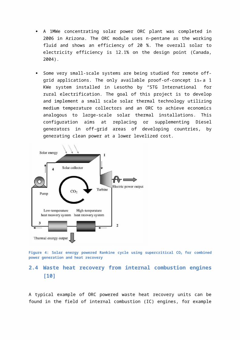
A coupling of the ORC process with internal combustion engines can be also found in first prototypes for on-road-vehicle applications, where the condition for waste heat is variable. Figure 5 shows the schematic setup of such a system.

Figure 5: Schematic representation of waste heat recovery for combustion engines

2.5 Industrial waste heat [22]

Heat recovery from ORC power plants can have many applications in the industrial sector, especially in fields where energy has an impact on the production process. Below is a list of potential fields for the ORC heat recovery systems.

2.5.1 Cement industry

The cement production process involves lime decarbonizing reactions, which being endothermic, requires great amounts of heat and high temperatures to take place.

The unused heat supplied for these reactions can be found in the combustion gas – or kiln gas – (after the raw material pre-heating) and in the clinker cooler air flow (an air stream used to cool down the clinker after it exits the kiln). These flows could, via thermal oil heat recovery circuits, be the heat sources feeding the ORC for power generation purposes.

Typical cement production plants have a production capacity between 2,000 and 8,000 tons per day, with energy consumption ranging from 3.5 to 5 GJ/ton of clinker produced (10%–15% of it in the form of electricity).

As an indication, the power that can be produced by a Turboden [14] ORC system in a typical cement making process can range from 0.5 to 1 MW/kilotons per day of clinker production capacity (assuming heat recovery from both kiln and cooler waste flows).

Using these figures, it can be estimated that the energy produced by an ORC can account for around 10%–20% of the total electricity consumed by a cement plant.

Additionally, in the case of heavy fuel oil (or similar liquid fuels) being used as a fuel (either primary or as a back-up), some of the recovered heat can also be used to keep the system at the correct working temperature.

2.5.2 Steel industry

In the steel production and processing industry, there are multiple waste heat sources where energy recovery with the ORC is possible. They can be divided into relatively ‘clean’ sources (fumes from rolling pre-heating furnaces, forging pre-heating furnaces, thermal treatments that are typically methane-fuelled and have a relatively low dust content) and relatively ‘unclean’ ones (fumes from blast furnaces, electric arc furnaces …).

For the clean sources, heat recovery processes can rely on established technology to interface with the process (heat recovery exchangers); the second option, the exhaust characteristics (very high flows, high temperatures, high dust content, large variations in operating loads, environmental constraints) requires significant development to be carried out on the heat recovery exchangers.

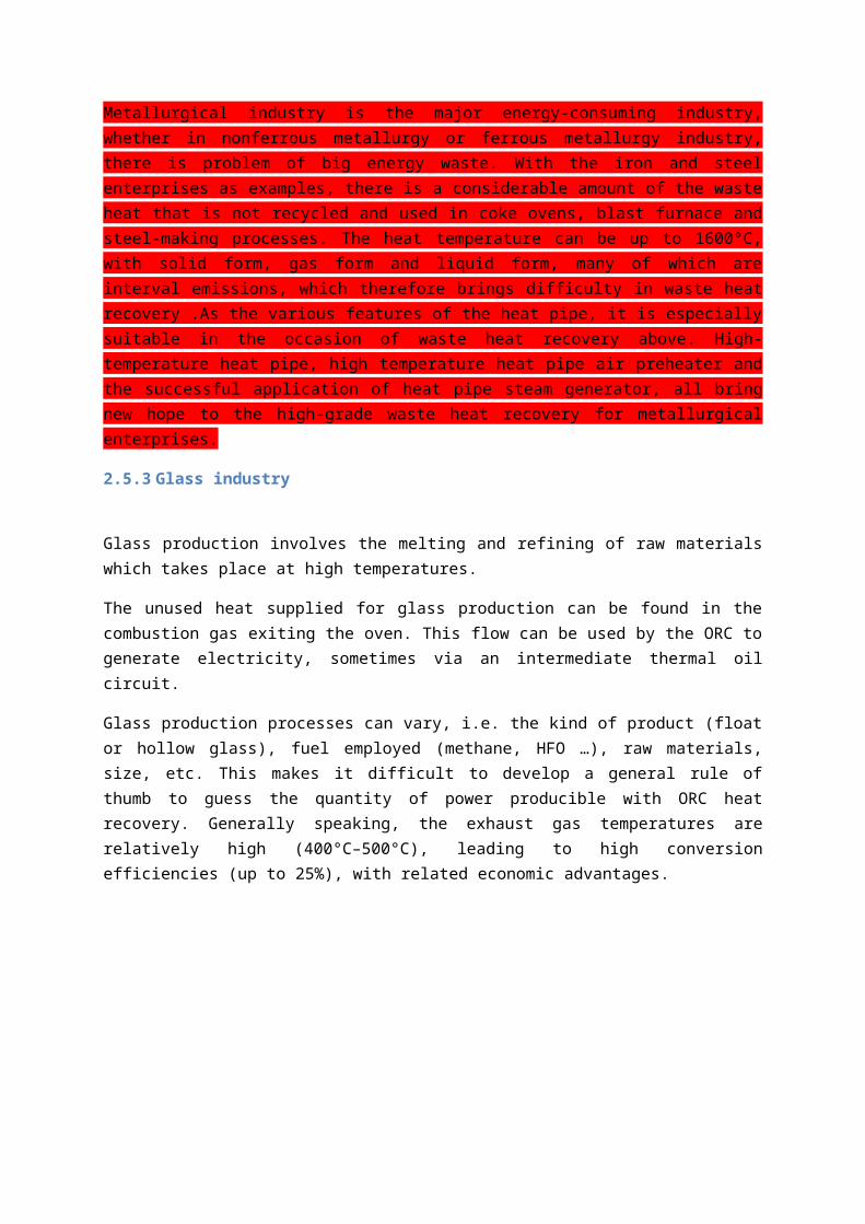
Metallurgical industry is the major energy-consuming industry, whether in nonferrous metallurgy or ferrous metallurgy industry, there is problem of big energy waste. With the iron and steel enterprises as examples, there is a considerable amount of the waste heat that is not recycled and used in coke ovens, blast furnace and steel-making processes. The heat temperature can be up to 1600°C, with solid form, gas form and liquid form, many of which are interval emissions, which therefore brings difficulty in waste heat recovery .As the various features of the heat pipe, it is especially suitable in the occasion of waste heat recovery above. High-temperature heat pipe, high temperature heat pipe air preheater and the successful application of heat pipe steam generator, all bring new hope to the high-grade waste heat recovery for metallurgical enterprises.

2.5.3 Glass industry

Glass production involves the melting and refining of raw materials which takes place at high temperatures.

The unused heat supplied for glass production can be found in the combustion gas exiting the oven. This flow can be used by the ORC to generate electricity, sometimes via an intermediate thermal oil circuit.

Glass production processes can vary, i.e. the kind of product (float or hollow glass), fuel employed (methane, HFO …), raw materials, size, etc. This makes it difficult to develop a general rule of thumb to guess the quantity of power producible with ORC heat recovery. Generally speaking, the exhaust gas temperatures are relatively high (400°C–500°C), leading to high conversion efficiencies (up to 25%), with related economic advantages.

Chapter 3 Transcritical organic Rankine cycle

1. Introduction

The ideal thermal efficiency of a power cycle operating between a constant heat source and cold source temperature is the Carnot efficiency, defined as follows:

ηC=|w|q¿

=q¿−|qout|

qout=TH−T L

T H=1−

T L

T H

The Carnot cycle consists of the four reversible processes shown in the T,s-diagram Figure 6. The processes are:

1→2: Isentropic expansion during which work is produced by the cycle working fluid 2→3: Isothermal heat rejection from the working fluid to a cooling medium 3→4: Isentropic compression during which work is performed on the cycle working fluid 4→1: Isothermal heat addition to the working fluid from a heating medium.

Figure 6: Ideal Carnot cycle

Due to the fact that in power production cycles, for example using waste heat, the heat source is cooled down in the heat exchange process, the Carnot-efficiency and the maximum amount of transferred heat are competing objectives (Figure 7).

Figure 7: Heat exchanger efficiency for a cooled down heat source, for a ideal Carnot cycle with Tmax = 130°C and 160°C [23].

DiPippo [24] reviewed the Carnot cycle to its appropriateness to serve as the ideal model for geothermal binary power plants. It was shown that the Carnot cycle sets an unrealistically high upper limit on the thermal efficiency of these plants. A more useful model is the triangular or trilateral cycle (Figure 8) because binary plants, for example operating on geothermal hot water, use a non-isothermal heat source. The triangular cycle imposes a lower upper bound on the thermal efficiency and serves as a more meaningful ideal cycle against which to measure the performance of real binary cycles.

Figure 8: Triangular cycle

The thermal efficiency of a triangular cycle is lower than the ideal Carnot cycle for the same upper and lower temperature.

The triangular cycle consists out of three processes (Figure 8):

The first two are the same as in the ideal Carnot cycle. The heating process (state point 3 to state point 1) now is non-isothermal.

The thermal efficiency of the ideal triangular cycle is defined by (DiPippo [24]):

ηthTri=

T H−T L

TH+T L

The cycle 1561 (Figure 8) represents the maximum-efficiency triangular cycle, given the temperature of the heat source and the prevailing dead-state temperature. The thermal efficiency for this cycle is:

ηth ,maxTri =

T H−T 0T H+T 0

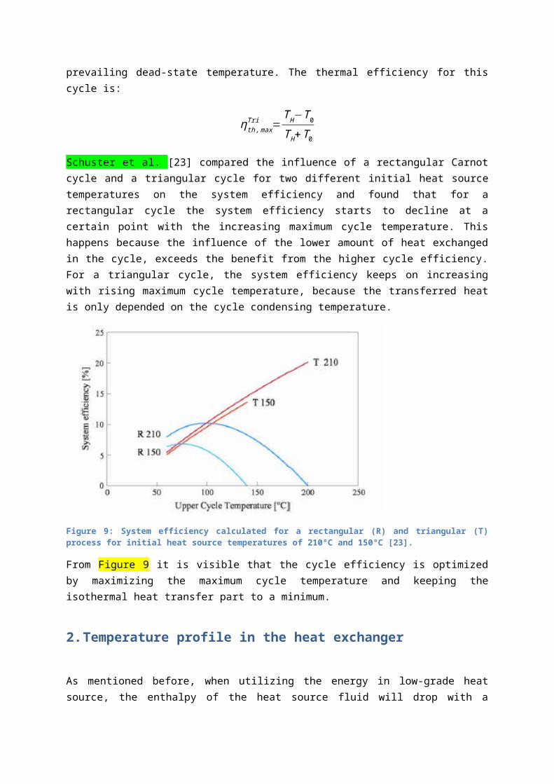
Schuster et al. [23] compared the influence of a rectangular Carnot cycle and a triangular cycle for two different initial heat source temperatures on the system efficiency and found that for a rectangular cycle the system efficiency starts to decline at a certain point with the increasing maximum cycle temperature. This happens because the influence of the lower amount of heat exchanged in the cycle, exceeds the benefit from the higher cycle efficiency. For a triangular cycle, the system efficiency keeps on increasing with rising maximum cycle temperature, because the transferred heat is only depended on the cycle condensing temperature.

Figure 9: System efficiency calculated for a rectangular (R) and triangular (T) process for initial heat source temperatures of 210°C and 150°C [23].

From Figure 9 it is visible that the cycle efficiency is optimized by maximizing the maximum cycle temperature and keeping the isothermal heat transfer part to a minimum.

2. Temperature profile in the heat exchanger

As mentioned before, when utilizing the energy in low-grade heat source, the enthalpy of the heat source fluid will drop with a gliding temperature profile in the main heat exchanger during the energy transfer process. Larjola et al. [25] pointed out that for a cycle that uses waste heat at a moderate inlet temperature (80–200°C) as heat source, the best efficiency and highest power output is usually obtained when the working fluid temperature profile can match the temperature profile of the heat source fluid. This means, the system will have a better performance if the temperature difference between the heat source and the temperature of the working fluid in an evaporator (or vapour generator) is reduced, because then the system has a lower irreversibility.

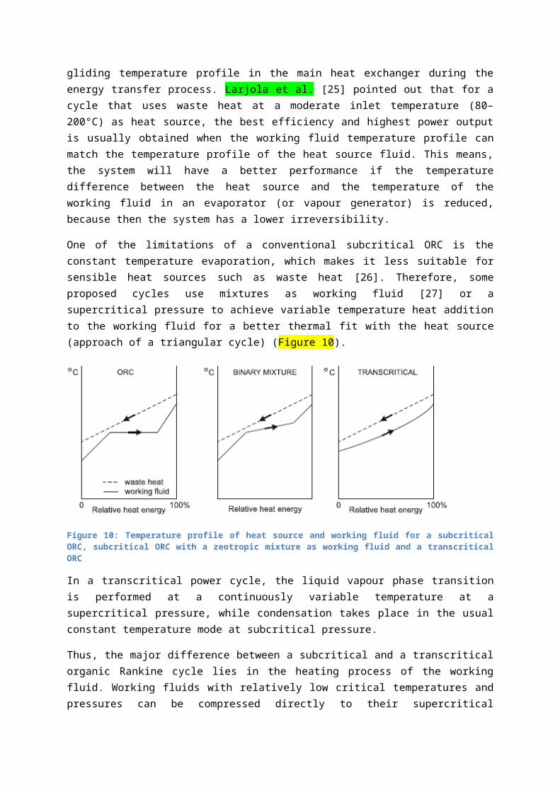
One of the limitations of a conventional subcritical ORC is the constant temperature evaporation, which makes it less suitable for sensible heat sources such as waste heat [26]. Therefore, some proposed cycles use mixtures as working fluid [27] or a supercritical pressure to achieve variable temperature heat addition to the working fluid for a better thermal fit with the heat source (approach of a triangular cycle) (Figure 10).

Figure 10: Temperature profile of heat source and working fluid for a subcritical ORC, subcritical ORC with a zeotropic mixture as working fluid and a transcritical ORC

In a transcritical power cycle, the liquid vapour phase transition is performed at a continuously variable temperature at a supercritical pressure, while condensation takes place in the usual constant temperature mode at subcritical pressure.

Thus, the major difference between a subcritical and a transcritical organic Rankine cycle lies in the heating process of the working fluid. Working fluids with relatively low critical temperatures and pressures can be compressed directly to their supercritical pressures and heated to their supercritical state, bypassing the two-phase region (no phase-transition). By bypassing the isothermal boiling process, the temperature-glide (temperature change during take-up of heat energy) of a transcritical Rankine cycle allows the working fluid to have a better thermal match with the heat source compared to a subcritical organic fluid, resulting in less exergy losses and exergy destruction. Furthermore, by avoiding the boiling process, the configuration of the heating system can be potentially simplified.

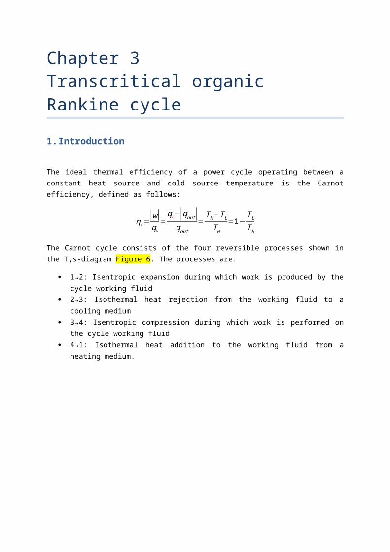
Figure 11 shows the different thermal match for R152a in a conventional organic Rankine cycle and R134a in a transcritical Rankine cycle for the same maximum temperature and pinch limitation [28].

Figure 11: Δ H -diagram demonstrating the thermal match in a subcritical and transcritical organic Rankine cycle. (a) Heating R152a in a subcritical ORC at 20 bar from 31.16°C to 100°C. (b) Heating R134a in a transcritical ORC at 40 bar from 33.93°C to 100°C [28].

The transcritical cycle, where heat rejection takes place at a subcritical pressure and heat addition at a supercritical pressure, must not be confused with the entirely supercritical cycle proposed by Feher[29].

Studies about low-temperature heat sources in transcritical cycles are quite rare and were first being considered for geothermal power generation (Gu et al. [30] [31]). Later, transcritical cycles have also been studied for solar energy (Zhang X.R. et al. [32] [33]) and waste heat applications (Chen Y et al. [34]).

3. The transcritical cycle

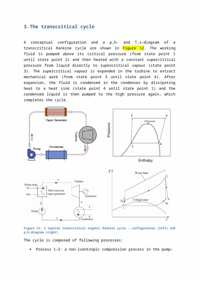
A conceptual configuration and a p,h- and T,s-diagram of a transcritical Rankine cycle are shown in Figure 12. The working fluid is pumped above its critical pressure (from state point 1 until state point 2) and then heated with a constant supercritical pressure from liquid directly to supercritical vapour (state point 3). The supercritical vapour is expanded in the turbine to extract mechanical work (from state point 3 until state point 4). After expansion, the fluid is condensed in the condenser by dissipating heat to a heat sink (state point 4 until state point 1) and the condensed liquid is then pumped to the high pressure again, which completes the cycle.

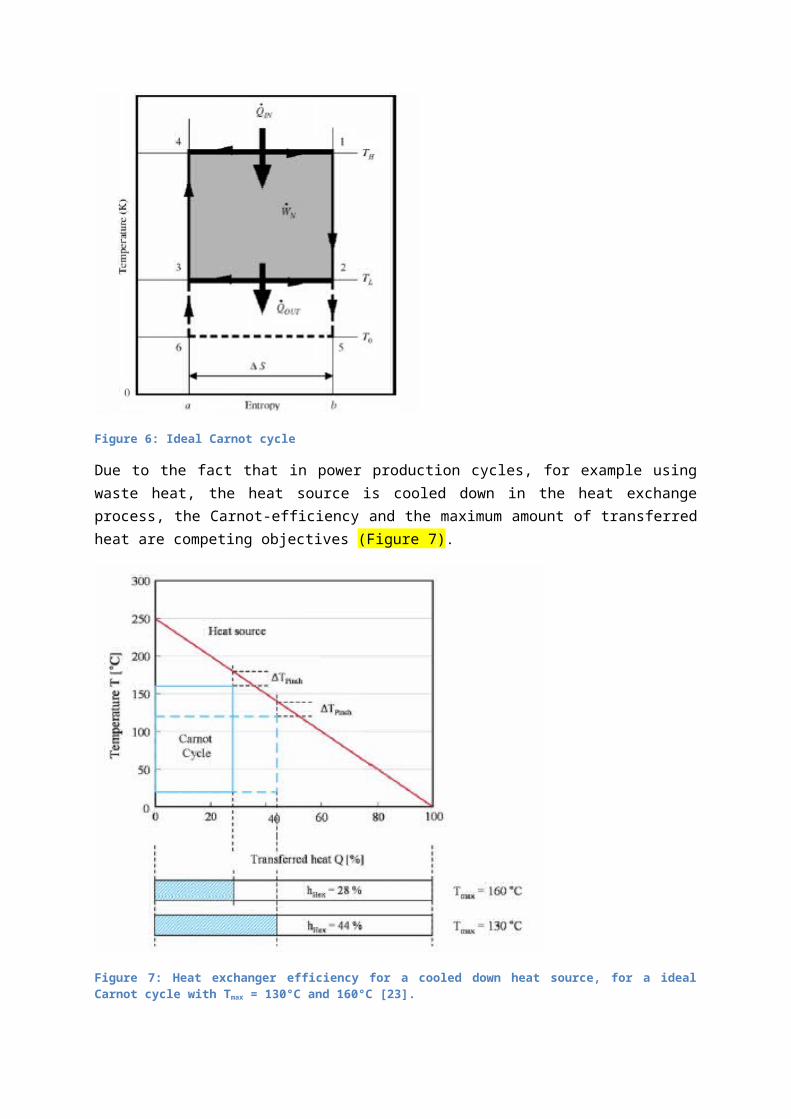
Figure 12: A typical transcritical organic Rankine cycle – configuration (left) and p,h-diagram (right)

The cycle is composed of following processes:

Process 1–2: a non-isentropic compression process in the pump; Process 2–3: a constant-pressure heat absorption process in the vapour generator; Process 3–4: a non-isentropic expansion process in the expander/turbine; Process 4–1: a constant-pressure heat rejection process in the condenser;

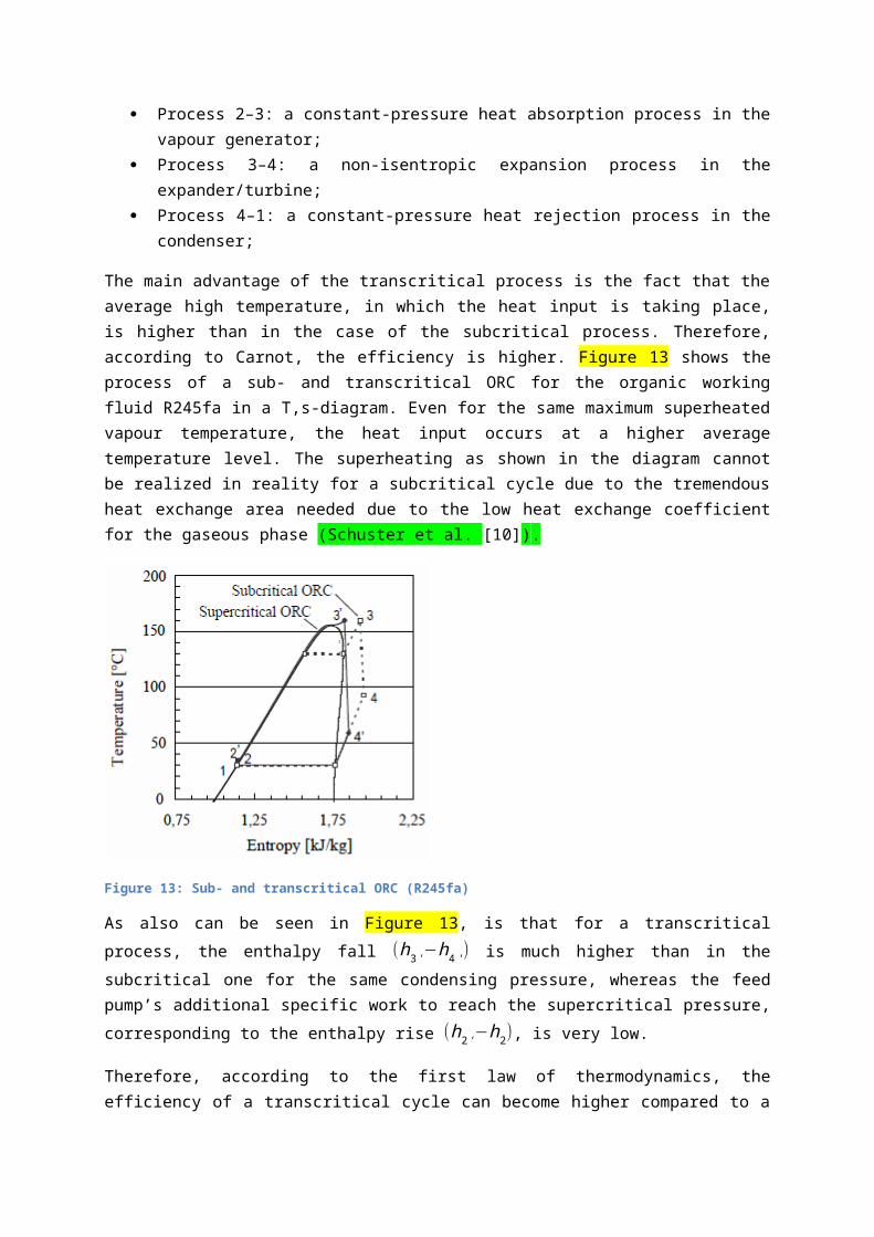
The main advantage of the transcritical process is the fact that the average high temperature, in which the heat input is taking place, is higher than in the case of the subcritical process. Therefore, according to Carnot, the efficiency is higher. Figure 13 shows the process of a sub- and transcritical ORC for the organic working fluid R245fa in a T,s-diagram. Even for the same maximum superheated vapour temperature, the heat input occurs at a higher average temperature level. The superheating as shown in the diagram cannot be realized in reality for a subcritical cycle due to the tremendous heat exchange area needed due to the low heat exchange coefficient for the gaseous phase (Schuster et al. [10]).

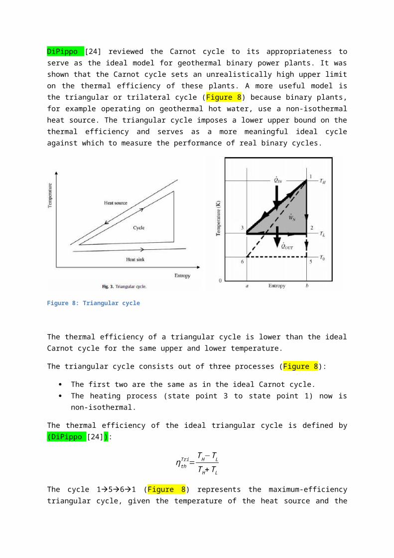
Figure 13: Sub- and transcritical ORC (R245fa)

As also can be seen in Figure 13, is that for a transcritical process, the enthalpy fall (h3 '−h4 ') is much higher than in the subcritical one for the same condensing pressure, whereas the feed pump’s additional specific work to reach the supercritical pressure, corresponding to the enthalpy rise (h2 '−h2), is very low.

Therefore, according to the first law of thermodynamics, the efficiency of a transcritical cycle can become higher compared to a subcritical cycle. Thus, if the heat transfer between the power cycle and the heat source is taken into account properly, a transcritical power cycle should have a better performance than a subcritical ORC.

Chapter 4 Classification of working fluids-Selection criteria

1. Introduction

The selection of working fluids and operating conditions are very important to the system performance. The thermodynamic properties of working fluids will affect the system efficiency and operation.

However, the thermodynamic parameters of the fluid are not the only criteria for selection of an appropriate working fluid. The Montreal Protocol on Substances that Deplete the Ozone Layer [35] and the EC regulation 2037/2000 restrict the use of ozone depleting substances (European Parliament and council, 2004). Therefore, the cycle designer should always be aware of the global warming potential and the low ozone depletion of the working fluid before designing the ORC-application.

In order to identify the most suitable organic fluids, several general criteria have to be taken into consideration, namely:

safety and health aspects:o toxicity (MAC = Maximum Allowable Concentration)o explosion limito flammabilityo small potential of decompositiono stability of the fluido compatibility with materials in contact (non-corrosive)

environmental aspects:o low ozone depletion potential (ODP)o low global warming potential (GWP)o low atmospheric life time

thermophysical aspects (shape of saturated vapour line, low critical pressure and temperature, high density, low viscosity, high thermal conductivity …)

thermodynamic aspects (efficiency, net power output, low specific volumes …) working range of waste heat (temperature, heat flux …) availability and cost of the working fluid cost of the system

The two main parameters for fluid selection are the maximum and minimum process temperature. The upper limit of the maximum process temperature is the fluid stability and material compatibility.

The melting temperature should be below ambient temperature, because else the fluid may solidify during shutdown time.

An important aspect for the choice of the working fluid is the temperature of the available heat source, which can range from low temperatures of about 90°C to medium temperatures of about 400°C for ORC-applications.

For low-temperature heat sources the advantage of organic fluids is obvious because of higher molecular mass and the volume ratio of the working fluid at the turbine outlet and inlet (or the vapour expansion ratio VER). The latter can be smaller by an order of magnitude for organic fluids than for water and thus allows the use of simpler and cheaper turbines [36].

2. Classification and selection criteria of working fluids

There is a wide selection of organic fluids which can be used in organic Rankine cycles. Despite all the research activities that are going on in this field, there is no consensus concerning the best working fluid. This is due to the fact that the working fluids have to be subjected to a number of criteria and also due to the wide range of applications. Refrigerants are the most promising fluids for ORC cycles according to Mago et al. [37], especially with the view of their low toxicity.

The fluid selection affects the system efficiency, operating conditions, environmental impact and economic viability. Selection criteria are set out in this section to locate the potential working fluid candidates for different cycles at various conditions. Some of these criteria can only be used after evaluation of the cycle by simulation. A difference can be made between criteria that can be evaluated without simulation of the cycle, called “screening criteria”, and criteria after simulation of the cycle, called “cycle criteria”. The working fluids will eventually be selected by a combination of all these criteria.

2.1 Screening criteria

2.1.1 Safety criterion (ASHRAE 34)

The American Society of Heating, Refrigerating and Air-Conditioning Engineers (ASHRAE) focuses on building systems, energy efficiency, indoor air quality, refrigeration and sustainability within the industry. ASHRAE also publishes a well-recognized series of standards and guidelines relating to HVAC systems and issues. The standard ASHRAE 34 describes the “Designation and Safety Classification of Refrigerants” and gives an indication of the safety level of the used refrigerant [38].

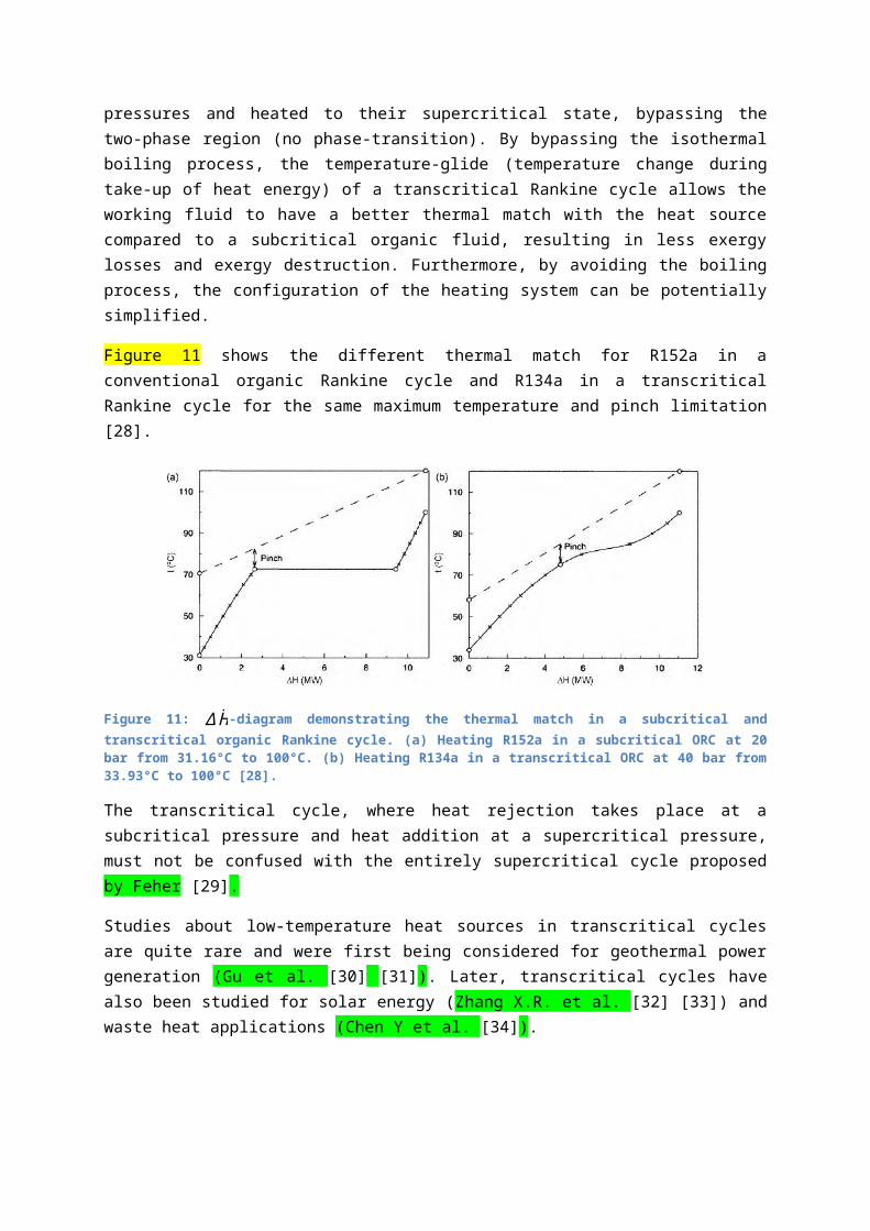
Table 3: The standard AHRAE 34 classification

Toxicity:

Class A represents refrigerants for which the toxicity has not been identified at concentrations less than or equal to 400 ppm by volume.

Class B represents refrigerants for which there is evidence of toxicity at concentrations below 400 ppm by volume.

Flammability:

Class 1 indicates refrigerants that do not show flame propagation when tested in air at 101.3 kPa and 21°C.

Class 2 represents refrigerants having a lower flammability limit (LFL) of more than 0.10 kg/m³ at 101.3 kPa and 21°C and the heat of combustion (HOC) less than 19 MJ/kg.

Class 3 represents refrigerants which are highly flammable and having a lower flammability limit (LFL) of less than 0.10 kg/m³ at 101.3 kPa and 21°C or the heat of combustion (HOC) greater than or equal to 19 MJ/kg.

2.1.2 Environmental criterion

The most important environmental criteria are the global warming potential (GWP), ozone depletion potential (ODP) and the atmospheric lifetime (ALT).

Global-warming potential (GWP) is a relative measure of how much heat a greenhouse gas traps in the atmosphere. It compares the amount of heat trapped by a certain mass of the gas in question to the amount of heat trapped by a similar mass of carbon dioxide. A GWP is calculated over a specific time interval, commonly 20, 100 or 500 years. For example, the 20 year GWP of methane is 72, which means that if the same mass of methane and carbon dioxide were introduced into the atmosphere, that methane will trap 72 times more heat than the carbon dioxide over the next 20 years [39].

The ozone depletion potential (ODP) of a chemical compound is the relative amount of degradation to the ozone layer it can cause, with trichlorofluoromethane (R11) being fixed at an ODP of 1. Chlorodifluoromethane (R22), for example, has an ODP of 0.055 x R11, or R11 has the maximum potential amongst chlorocarbons because of the presence of three chlorine atoms in the molecule [40].

The atmospheric lifetime (ATL) of a chemical compound is the period of time required to restore the equilibrium after a sudden increase or decrease in its concentration in the atmosphere. The time

depends on the chemical reactions that the gas goes through and the natural buffering capabilities. Individual atoms or molecules may be lost or deposited to sinks such as the soil, the oceans and other waters, or vegetation and other biological systems, reducing the excess to background concentrations [41].

An important statement here, as mentioned before, is the Montreal Protocol [35]. This determines the phasing out of chlorofluorocarbon (CFC) and hydrochlorofluorocarbon compounds (HCFC). The use and production of CFCs has been banned since 2010. For HCFCs the following transition rules are:

2004: reduction of 35% from the reference; 2010: reduction of 75% from the reference; 2015: reduction of 90% from the reference; 2020: reduction of 99.5% from the reference; 2030: complete phase out.

The reference for developed countries is set at 2.8% of that country's 1989 chlorofluorocarbon consumption + 100% of that country's 1989 HCFC consumption [35].

Some working fluids have been phased out, such as R11, R12, R113, R114, and R115, while some others are being phased out in 2020 or 2030 (such as R21, R22, R123, R124, R141b and R142b).

READ 2007 ADJUSTMENTS TO ADD TO TEXT (SEE REFRIGERANTS)

The hydrofluorocarbons (HFCs: a compound consisting of hydrogen, fluorine, and carbon) are a class of replacements for CFCs. Because they do not contain chlorine or bromine, they do not deplete the ozone layer. All HFCs have an ozone depletion potential of 0, but some of them have a high GWP!

The ORC system can take the advantage of reducing the consumption of fossil fuels and the emission of the greenhouse gas.

For example if a geothermal power plant is used instead of a petroleum-fired power plant, the saved petroleum (M pe in kiloliter/year) and reduced CO2 emission (M em in kg/year) per year can be simply estimated as [42]:

M pe=365t 0ape (W exp−W pump−W pump ,CS−W pump,WH )

M em=365t 0aem (W exp−W pump−W pump,CS−W pump,WH )

Where:

t 0 is the operating time per day (e.g. 24h);

a pe is the amount of petroleum consumed to produce 1 kWh of electrical energy (e.g. 0.266

l/kWh); aem is the amount of CO2 emission if 1 kWh of electrical energy produced by a petroleum fire

power plant (e.g. 0.894 kg/kWh).

2.1.3 Stability of the working fluid and compatibility with materials in contact

Unlike water, organic fluids usually suffer chemical deterioration and decomposition at high temperatures [43]. The maximum operating temperature is thus limited by the chemical stability of the working fluid. Additionally, the working fluid should be noncorrosive and compatible with engine materials and lubricating oil. Calderazzi and Paliano [44] studied the thermal stability of R134a, R141b, R13I1, R7146 and R125 associated with stainless steel as the container material. Andersen and Bruno [9] presented a method to assess the chemical stability of potential working fluids by ampule testing techniques. The method allows the determination of the decomposition reaction rate constant of simple fluids at the temperatures and pressures of interest.

2.1.4 Thermophysical properties

The several thermophysical properties for evaluation of the suitability of a working fluid for ORC-applications are:

the type of fluids; the influence of latent heat, density and specific heat; the critical temperature and pressure; the use of mixtures as working fluid; and the availability and cost of the working fluids.

2.1.4.1 Type of fluids

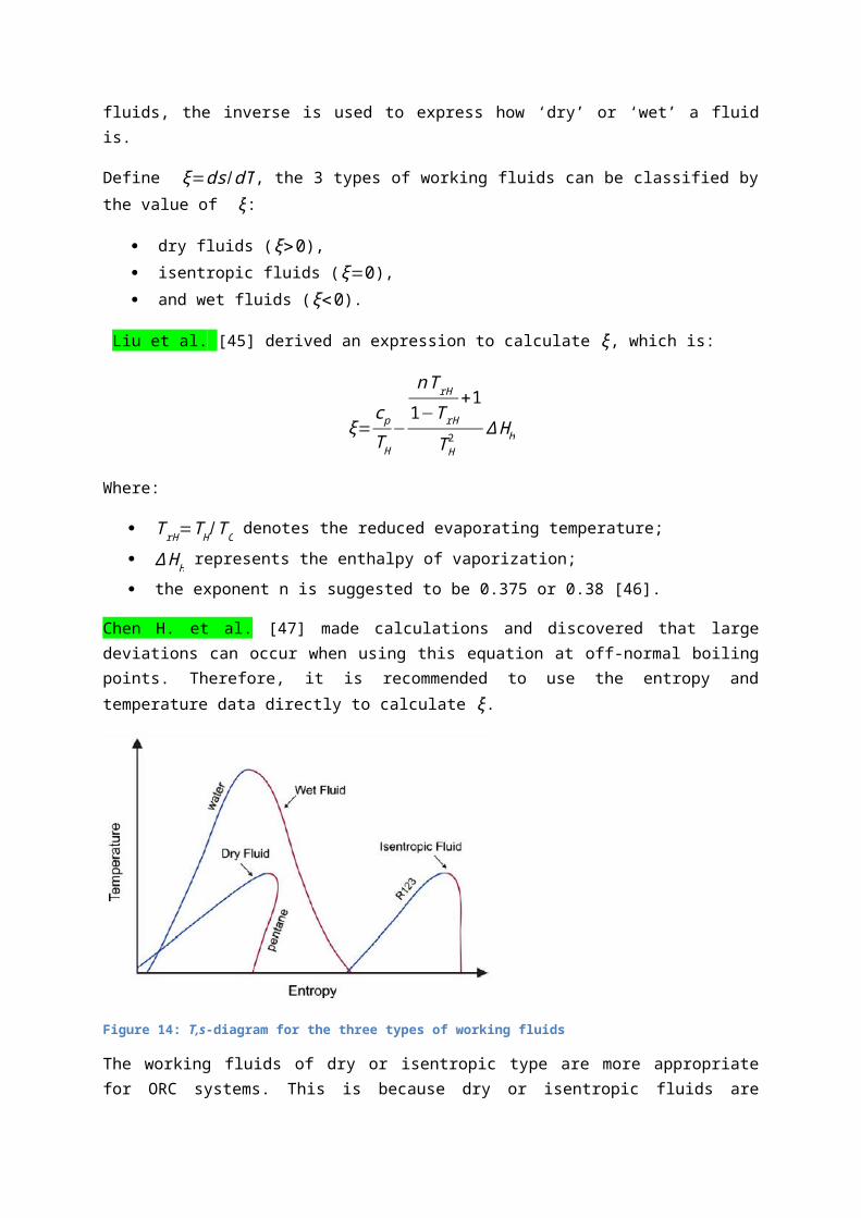
The working fluids can be classified into three categories according to the shape of the saturated vapour line in the T,s-diagram (Figure 14). Since the value of dT /ds leads to infinity for isentropic fluids, the inverse is used to express how ‘dry’ or ‘wet’ a fluid is.

Define ξ=ds/dT , the 3 types of working fluids can be classified by the value of ξ :

dry fluids (ξ>0), isentropic fluids (ξ=0), and wet fluids (ξ<0).

Liu et al. [45] derived an expression to calculate ξ , which is:

ξ=cp

TH−

nT rH

1−T rH+1

T H2 ΔHH

Where:

T rH=T H /TC denotes the reduced evaporating temperature;

ΔH H represents the enthalpy of vaporization;

the exponent n is suggested to be 0.375 or 0.38 [46].

Chen H. et al. [47] made calculations and discovered that large deviations can occur when using this equation at off-normal boiling points. Therefore, it is recommended to use the entropy and temperature data directly to calculate ξ .

Figure 14: T,s-diagram for the three types of working fluids

The working fluids of dry or isentropic type are more appropriate for ORC systems. This is because dry or isentropic fluids are superheated after isentropic expansion, thereby eliminating the concerns of impingement of liquid droplets on the turbine blades. However, if the liquid is “too dry”, the expanded vapour will leave the turbine with substantial superheat, which is a waste and adds to the cooling load in the condenser [48]. The cycle efficiency can be increased using this superheat to preheat the liquid after it leaves the feed pump and before it enters the vapour generator.

Liu et al. [45] investigated the effect of working fluids in organic Rankine cycles for waste heat recovery and found that the presence of a hydrogen bond in certain molecules such as water, ammonia and ethanol may result in ‘wet’ fluid conditions due to larger vaporizing enthalpy, and is regarded unsuitable for ORCs.

Furthermore, it can be observed from literature, that the fluids consisting of simpler molecules are mostly of the ‘wet’ type, while those consisting of more complicated molecules are mostly of the ‘dry’ type (BRON).

In the next paragraphs the basic types of organic Rankine cycles will be described according to the type of working fluid. The state points of the used T,s-diagrams (Figure 16 and Figure 18) correspond with the cycle architecture of Figure 15.

Figure 15: Organic Rankine Cycle a) without IHE b) with IHE

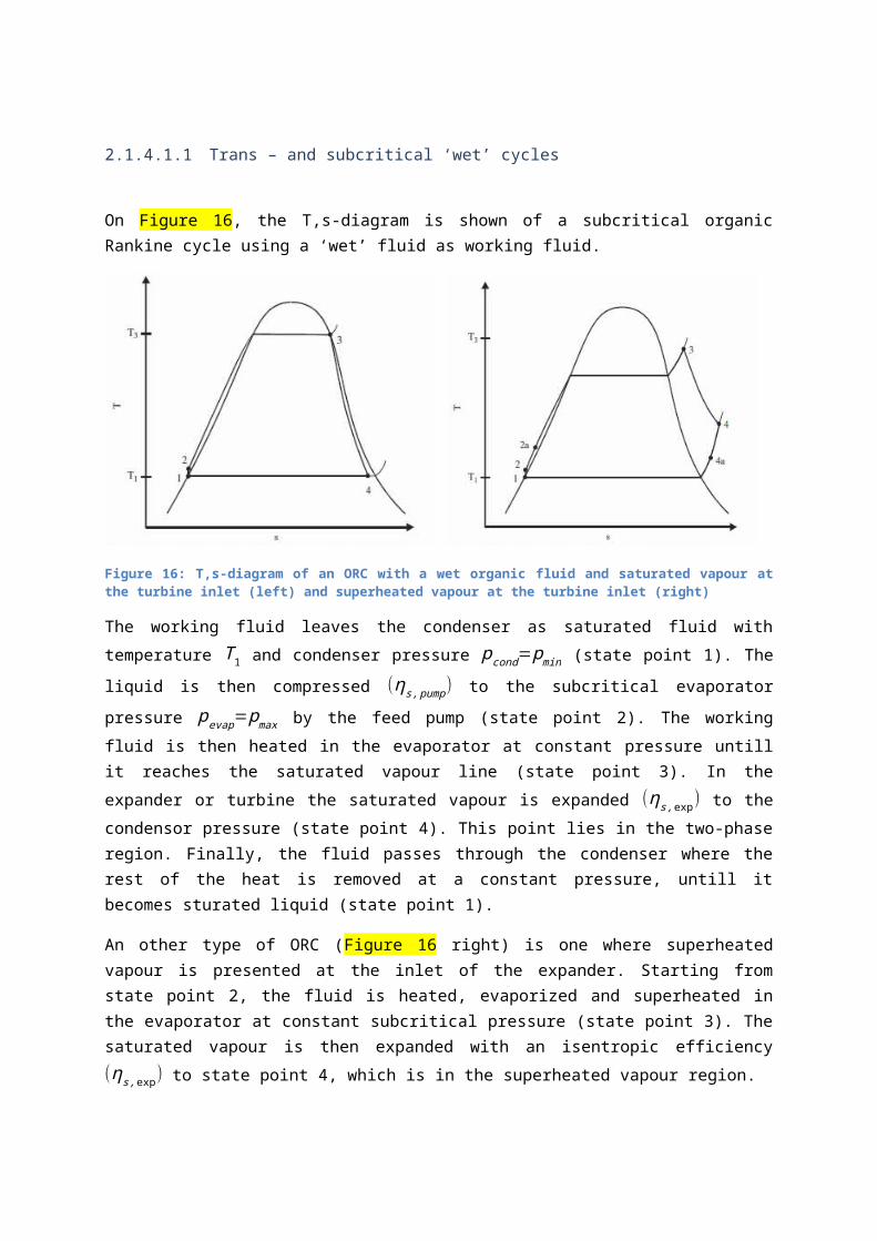
2.1.4.1.1 Trans – and subcritical ‘wet’ cycles

On Figure 16, the T,s-diagram is shown of a subcritical organic Rankine cycle using a ‘wet’ fluid as working fluid.

Figure 16: T,s-diagram of an ORC with a wet organic fluid and saturated vapour at the turbine inlet (left) and superheated vapour at the turbine inlet (right)

The working fluid leaves the condenser as saturated fluid with temperature T 1 and condenser pressure pcond=pmin (state point 1). The liquid is then compressed (η s , pump) to the subcritical evaporator pressure pevap=pmax by the feed pump (state point 2). The working fluid is then heated in the evaporator at constant pressure untill it reaches the saturated vapour line (state point 3). In the expander or turbine the saturated vapour is expanded (ηs ,exp) to the condensor pressure (state point

4). This point lies in the two-phase region. Finally, the fluid passes through the condenser where the rest of the heat is removed at a constant pressure, untill it becomes sturated liquid (state point 1).

An other type of ORC (Figure 16 right) is one where superheated vapour is presented at the inlet of the expander. Starting from state point 2, the fluid is heated, evaporized and superheated in the evaporator at constant subcritical pressure (state point 3). The saturated vapour is then expanded with an isentropic efficiency (ηs ,exp) to state point 4, which is in the superheated vapour region.

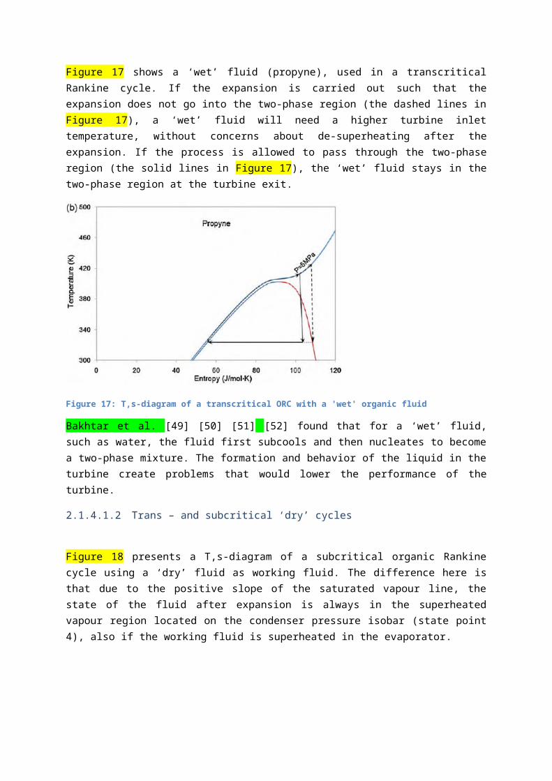
Figure 17 shows a ‘wet’ fluid (propyne), used in a transcritical Rankine cycle. If the expansion is carried out such that the expansion does not go into the two-phase region (the dashed lines in Figure17), a ‘wet’ fluid will need a higher turbine inlet temperature, without concerns about de-superheating after the expansion. If the process is allowed to pass through the two-phase region (the solid lines in Figure 17), the ‘wet’ fluid stays in the two-phase region at the turbine exit.

Figure 17: T,s-diagram of a transcritical ORC with a 'wet' organic fluid

Bakhtar et al. [49] [50] [51] [52] found that for a ‘wet’ fluid, such as water, the fluid first subcools and then nucleates to become a two-phase mixture. The formation and behavior of the liquid in the turbine create problems that would lower the performance of the turbine.

2.1.4.1.2 Trans – and subcritical ‘dry’ cycles

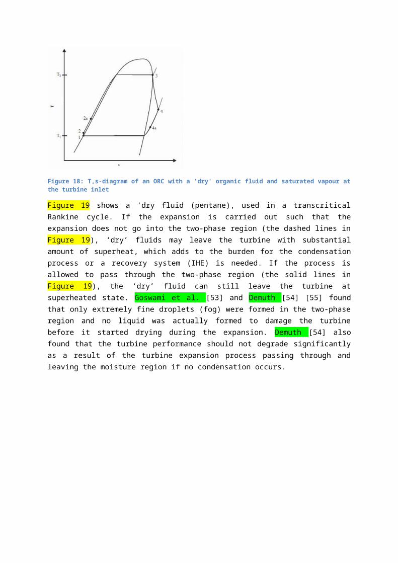
Figure 18 presents a T,s-diagram of a subcritical organic Rankine cycle using a ‘dry’ fluid as working fluid. The difference here is that due to the positive slope of the saturated vapour line, the state of the fluid after expansion is always in the superheated vapour region located on the condenser pressure isobar (state point 4), also if the working fluid is superheated in the evaporator.

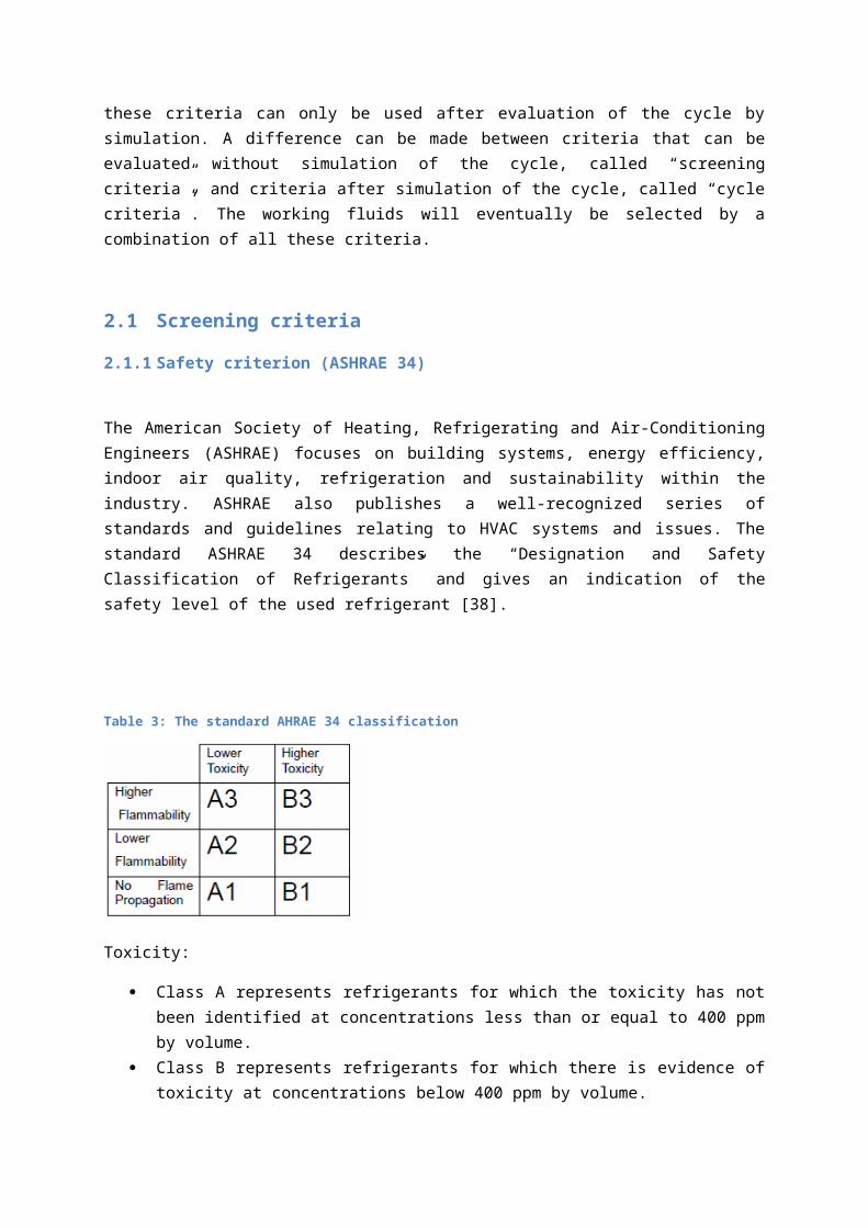
Figure 18: T,s-diagram of an ORC with a 'dry' organic fluid and saturated vapour at the turbine inlet

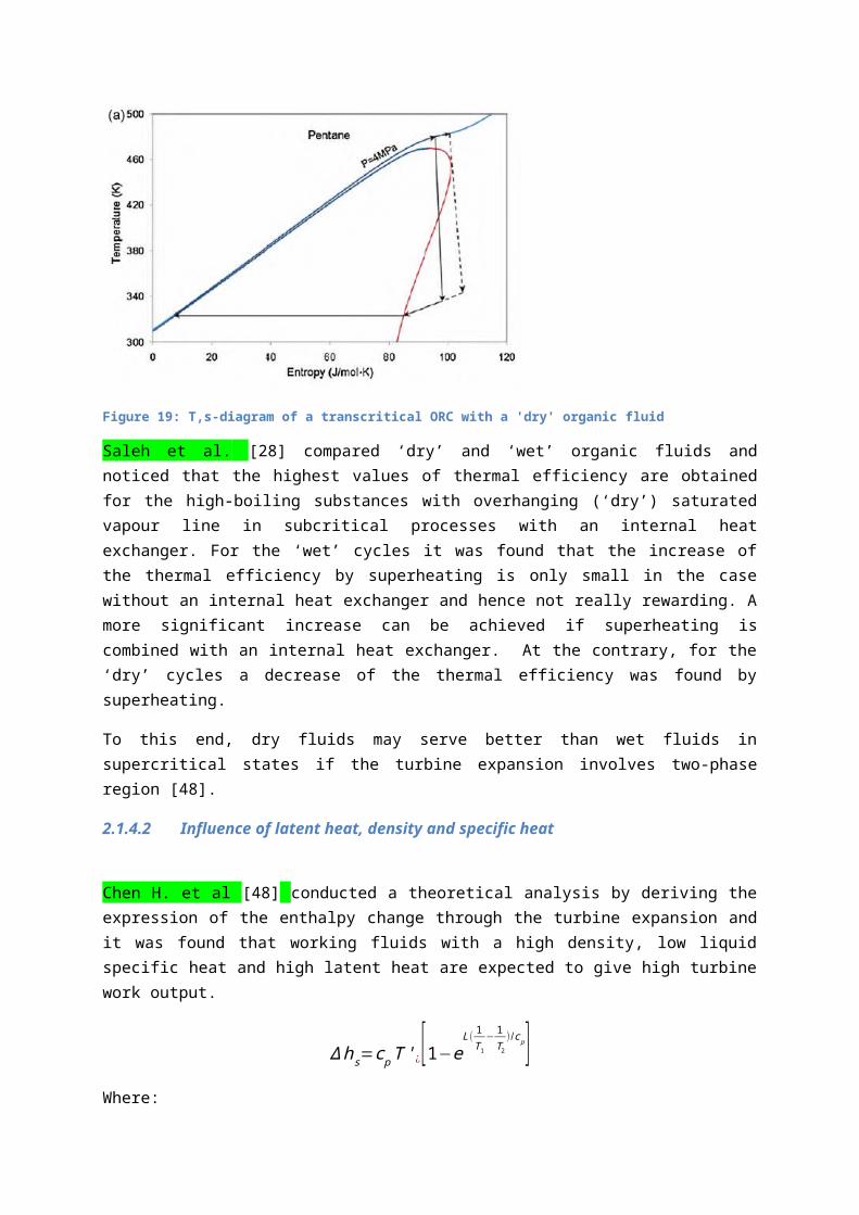
Figure 19 shows a ‘dry fluid (pentane), used in a transcritical Rankine cycle. If the expansion is carried out such that the expansion does not go into the two-phase region (the dashed lines in Figure 19), ‘dry’ fluids may leave the turbine with substantial amount of superheat, which adds to the burden for the condensation process or a recovery system (IHE) is needed. If the process is allowed to pass through the two-phase region (the solid lines in Figure 19), the ‘dry’ fluid can still leave the turbine at superheated state. Goswami et al. [53] and Demuth [54] [55] found that only extremely fine droplets (fog) were formed in the two-phase region and no liquid was actually formed to damage the turbine before it started drying during the expansion. Demuth [54] also found that the turbine performance should not degrade significantly as a result of the turbine expansion process passing through and leaving the moisture region if no condensation occurs.

Figure 19: T,s-diagram of a transcritical ORC with a 'dry' organic fluid

Saleh et al. [28] compared ‘dry’ and ‘wet’ organic fluids and noticed that the highest values of thermal efficiency are obtained for the high-boiling substances with overhanging (‘dry’) saturated vapour line in subcritical processes with an internal heat exchanger. For the ‘wet’ cycles it was found that the increase of the thermal efficiency by superheating is only small in the case without an internal heat exchanger and hence not really rewarding. A more significant increase can be achieved

if superheating is combined with an internal heat exchanger. At the contrary, for the ‘dry’ cycles a decrease of the thermal efficiency was found by superheating.

To this end, dry fluids may serve better than wet fluids in supercritical states if the turbine expansion involves two-phase region [48].

2.1.4.2 Influence of latent heat, density and specific heat

Chen H. et al [48] conducted a theoretical analysis by deriving the expression of the enthalpy change through the turbine expansion and it was found that working fluids with a high density, low liquid specific heat and high latent heat are expected to give high turbine work output.

Δ hs=cpT ' ¿[1−eL(1T1

−1T 2

)/ cp]Where:

T1 and T2 are the saturation temperatures of two points on the coexistence line and T1 > T2; T’in is the turbine inlet temperature; and L is the latent heat.

2.1.4.3 Critical temperature and pressure

Besides the shape of the saturated vapour line, the pressure at which the working fluid exchanges heat is also an important classification parameter. A difference can be made between subcritical and transcritical cycles.

For a subcritical cycle, the working fluid undergoes a liquid-vapour phase transition, while for the transcritical cycle such a phase transition does not occur (Figure 20).

Figure 20: T,s-diagram - comparison between a sub- and supercritical fluid

In order to reject heat to the ambient in the condenser, the critical temperature must be above 300K (design condensation temperature). Furthermore, the critical point of a working fluid should not be too high to use in transcritical Rankine cycles.

Moreover, as in general, the molecularly simpler fluids have lower critical temperatures T crit, so lower T crit can be found for mostly ‘wet’-fluids and for higher T crit mostly ‘dry’-fluids (BRON).

2.1.4.4 Mixtures

As mentioned in Chapter 3 – section 2 Temperature profile in heat exchanger, mixtures of working fluids [27] can be used to achieve variable temperature heat addition in the vapour generator and heat rejection in the condenser for a better thermal fit with the heat source (cfr. triangular cycle).

Chen H. et al. [47] [56] stated that the use of zeotropic mixtures can approach an “ideal” working fluid for transcritical ORCs, as these mixtures have the property of a temperature-glide during phase-change, which decreases the exergy destruction during condensation.

Figure 21: A transcritical Rankine cycle with an "ideal" working fluid

A comparison between subcritical R134a and a transcritical zeotropic mixtures of R32 and R134a (0.3/0.7 mass fraction) shows that due to the thermal glide the zeotropic mixtures has a 22.67% higher exergy efficiency during the condensation process than pure R134a (Chen H. et al. [56]).

Figure 22: Condensing process of R134a (left) and the zeotropic mixture of R134a and R32 (right) and their thermal match with the cooling fluid .

2.1.5 Availability and cost of working fluids

The availability and cost of the working fluids are among the considerations when selecting working fluids. Traditional refrigerants used in organic Rankine cycles are expensive. This cost could be reduced by a more massive production of those refrigerants, or by the use of low cost hydrocarbons.

2.2 Cycle criteria - Selection by performance indicator

In order to choose an appropriate working fluid and operating conditions for a waste heat stream with a specific temperature and mass flow rate, several indicators have to be evaluated. A distinction can be made between thermodynamic indicators, heat exchanger design indicators and economic indicators.

2.2.1 Thermodynamic performance indicators

Using the first and second law of thermodynamics [57], a first performance evaluation can already be made of an organic Rankine cycle under diverse working conditions for different working fluids. The state points correspond with the organic Rankine cycle of Figure 15.

2.2.1.1 First law efficiency - Thermal efficiency of the cycle – Net power output

The thermal efficiency of the cycle is defined as the net mechanical power produced with an ORC to the heat input to the working fluid of the ORC.

η I=η th=Pnet

QOrganic fluid=

W net

Q2−3

The net mechanical power produced with an ORC can be written as:

Pnet=W net

¿W exp−|W pump|

¿W 3−4−W 1−2

¿ mORC [ (h3−h4 )− (h2−h1) ]

With (h3−h4 ) the enthalpy fall in the expander and (h2−h1 ) the enthalpy rise necessary for pumping the working fluid.

The heat input to the working fluid of the ORC by heat exchange in the vapour generator is equal to:

QOrganic fluid=Q2−3

¿ mORC (h3−h2 )

For an ORC with an internal heat exchanger or regenerator the input heat is given as:

Q2a−3=mORC (h3−h2a )

Working with a regenerator, the average temperature of heat transfer to the cycle (from T 2a to T 3) is higher than without IHE (from T 2 to T 3) while the average temperature of heat transfer to the

environment (from T 4a to T 1) is lower than in case without IHE (from T 4 to T 1). Also the heat transferred in the regenerator does not need to be supplied from outside. All these aspects result according to Carnot in a higher thermal efficiency.

Much research has been conducted on the ORC system using the first law as a selection criterion. Saleh et al. [28] screened 31 pure component working fluids for ORCs and noticed a general trend that the thermal efficiency increases with the fluids critical temperature.

Chen Y. et al. [58] compared a carbon dioxide transcritical power cycle with a subcritical ORC using R123 as working fluid for low-grade waste heat recovery (exhaust gas of 150° and a mass flow rate of 0.4 kg/s) and found that the transcritical CO2 cycle has a higher system efficiency when taking into account the heat transfer behaviour between the heat source and the working fluid. Furthermore, the transcritical CO2 cycle shows a higher power output, when using the same thermodynamic mean heat-rejection temperature of 25°C. The thermodynamic mean temperature is used as reference, because of non-isothermal heat addition and rejection. They also noted that only comparing the thermodynamic efficiencies of cycles might be misleading, since the highest power output is not achieved at maximum cycle thermal efficiency when utilizing a certain heat source.

Gu et al. [30] [31]) compared propane, R125 and R134a in a transcritical cycle for geothermal power generation by optimization of the cycle state parameters, especially the condensing temperatures or pressures. Propane and R134a are found to be more suitable as the working fluids of transcritical cycles because of their higher power output from the same geothermal resource compared to R125.

Baik et al. [59] compared optimized cycles of transcritical CO2 and R125 with the power output as objective function for a low-grade heat source of 100°C. They were also one of the first who took the pressure drop characteristics into account and didn’t fix the cycle minimum temperature, as in actual practice. A simple double-pipe heat exchanger was chosen for convenience under the assumption that if the working fluid performs better in a double-pipe heat exchanger it will perform better in other types of heat exchangers. It was found that R125 has around 14% more net power than CO2, because the CO2 cycle requires a higher pumping due to the higher pressure. Even though, CO 2 has better heat transfer and pressure drop characteristics. It should be noted that if a conventional approach, in which the cycle minimum temperature is fixed, were employed, the performance of the R125 cycle would be overestimated.

It can be concluded that in a lot of cases the overall thermal efficiency can be improved using transcritical cycles instead of subcritical cycles (e.g. +5% [60]), but this also happens at the expense of a bigger vapour generator (Mickielewicz et al. [60]).

As the thermal efficiency cannot reflect the ability to convert energy from low-grade waste heat into usable work, we need to consider the exergy efficiency, which can evaluate the performance for waste heat recovery.

2.2.1.2 Second law efficiency - Exergy efficiency

From the viewpoint of the first law of thermodynamics and energy conservation, used to determine the overall thermal efficiency, work and heat are equivalent. On the other hand, based on the second law of thermodynamics, exergy quantifies the difference between work and heat in terms of

irreversibility. Because of the thermodynamic irreversibility occurring in each of the components, such as non-isentropic expansion, non-isentropic compression and heat transfer over a finite temperature difference, the exergy analysis method can be employed to evaluate the performance for low-grade waste heat recovery.

Consider p0 and T0 to be the ambient pressure and temperature as the specified dead reference state. In most of the studies the conditions of the ambient environment are taken as the dead state.

The following assumptions are made to calculate the exergy of each state point:

It is assumed that only physical exergies are used for flue gas and steam flows. Chemical exergies of the substances are neglected. Kinetic and potential exergies of materials are ignored.

The exergy of the state point can be considered as [57]:

Ei=m [ (hi−h0 )−T 0 ( si−s0 ) ]

The exergy balance for an open thermodynamic system can be expressed as [57]:

∑ E input−∑ Eoutput=I

With I the exergy destruction or irreversibility.

The objective of this parameter is to show the use of the exergy concept in assessing the effectiveness of energy source utilization.

Exergy efficiency indicates the percentage of usable energy conserved during a process (e.g. condensation or heating process).

In literature several equations can be found for defining the exergy efficiency. The most three most suitable definitions are discussed below (Ho et al. [61]).

The internal second law efficiency η II ,∫¿¿ is defined as the ratio of the net work produced to the

potential work (or exergy) added [61].

ηII ,∫¿=

W net

mORC (eORC ,3−eORC ,2)¿

With eORC ,2 and eORC ,3 the specific exergy of the working fluid before and after heat addition, respectively.

The major problem with this equation is that it doesn’t give a good representation of the performance of the cycle in a waste heat recovery system, because the exergy in the heat source stream is afterwards discarded or not used anymore (the amount of unused exergy or exergy loss is noted as e loss).

Since the focus of this work is on waste heat recovery, the aim should be to optimize the heat transfer from the waste heat source to the working fluid and simultaneously optimize the net output power from this heat transfer.

The internal second law only says something about how efficient the cycle produces work from a certain amount of exergy that is added to the system during the heat addition, but it doesn’t say something about how efficient the cycle is at absorbing the exergy from the waste heat source.

In other words, a cycle can have a high internal second law efficiency, but only producing little power because only a small amount of exergy is added to the system.

If the heat energy of the heat source is still to be used after the heat transfer process to the power cycle (e.g. in combined heat and power cycles), it is better to define a second law efficiency that also includes the exergy destruction due to the heat transfer from the heat source to the working fluid.

η II , ext=W net

mHS ¿¿

This is also called the external second law efficiency [61].

For applications where the energy of the heat source is unused after the heat transfer process (e.g. some waste heat and solar power applications), the remaining exergy will eventually be lost to the environment. In this case it is better to define a more appropriate parameter that expresses the ratio of how much power is produced to the theoretical amount of potential work from a given finite heat source. This parameter is also called the utilisation efficiency [61].

η II ,ut=W net

mHS ¿¿

Where eHS ,0 represents the heat source’s exergy at the dead state.

The advantage of this non-dimensional parameter is that is can be used to compare different cycles.

The heat addition exergy efficiency can be defined as:

η II , add=mORC (eORC ,3−eORC ,2 )

mHS ¿¿

From Eq… and Eq…, the utilisation efficiency can also be written as [61]:

η II ,ut=η II ,∫¿ηII ,add ¿

It is clear that the utilisation efficiency can be maximized when the system is efficient at absorbing

heat energy (η II , add) and simultaneously efficient at concerting it to useful work (η II ,∫¿¿).

Several authors use different definitions for exergy efficiency, which makes it difficult to make a comparison between efficiencies listed in papers. An overview is listed below:

Cayer et al. [62]

ηex=1−Ed, tot

E¿, WH

With Ed ,tot the total exergy destruction:

Ed ,tot=∑im¿ e¿−∑

imout eout−W

Wang et al. [63]

ηex=E ¿,WH−∑ I−Eloss

E ¿,WH

With ∑ I the total system irreversibility and Eloss the exergy losses to the environment:

Eloss=Eout ,WH+ Eout ,CS

Chen H et al. [47]

ηex=W net

Eh+ Ep

With Eh the exergy of the working fluid obtained by absorbing heat from the heat source and Ep the exergy input by the pump.

Zhang XR et al. [64]

η II=ηI

ηideal

❑⇒ηII=

ηth

1−T0 /TWH

(BRON)

1ηII

=1+EDF total

With

EDF total=EDF pump+EDFvap−gen+EDF turbine+EDFcondenser

Schuster and Karellas (2010) [23] studied the efficiency optimization potential in transcritical ORCs for various working fluids (water, R1234a, R227ea, R152a, RC318, R236fa, iso-butene, R245fa, R365mfc, iso-pentane, iso-hexane and cyclo-hexane) and found that an improvement of about 8% in system efficiency is possible due to a better exergy efficiency. Furthermore it was also noticed that good system efficiencies and low exergy losses are not directly followed by low values for the heat transfer capacity UA.

Chen H. et al (2011) [47] performed an energetic and exergy analysis of a CO2- and R32 based transcritical Rankine cycle. R32 has the advantage that it has a higher thermal conductivity and condenses more easily than CO2. Furthermore, the thermal efficiency of R32 was about 12.6-18.7% higher than CO2 and works at much lower pressures. The exergy efficiency of R32 was also found to be higher over a wide range of the maximum pressure of the cycle.

2.2.1.2.1 System total irreversibility

Irreversibility is the cause of inefficiency and exergy loss/destruction. An exergetic analysis is necessary to know the extent of irreversibility in each process, and therefore the potential for improvement.

The work developed by the overall system can be written as [57]:

W c= (U−U 0 )+ p0 (V −V 0 )−T0 (S−S0 )+KE+PE−T 0σc

The exergy change of the system can be written as [57]:

E2−E1=(U 2−U1 )+ p0 (V 2−V 1 )−T 0 (S2−S1 )+(KE2−KE1)+(PE 2−PE1 )

Energy and entropy balance for a closed system can be written as [57]:

ΔU+ΔKE+ΔPE=∫1

2

δQ−W

ΔSentropychange

¿¿

The closed system exergy balance can then be written as [57]:

E2−E1=∫1

2

δQ−W+ p0 (V 2−V 1)−T 0 (S2−S1 )

Eq…⇒

E2−E1=∫1

2

δQ−T 0 (S2−S1 )−[W− p0 (V 2−V 1 ) ]

Eq…⇒

E2−E1=∫1

2

δQ−T 0[∫12

( δQT )b+σ ]−[W−p0 (V 2−V 1 ) ]

❑⇔

E2−E1exergychange

¿¿

The aim is to minimise the exergy destruction or irreversibility ( I=Ed ) of each component.

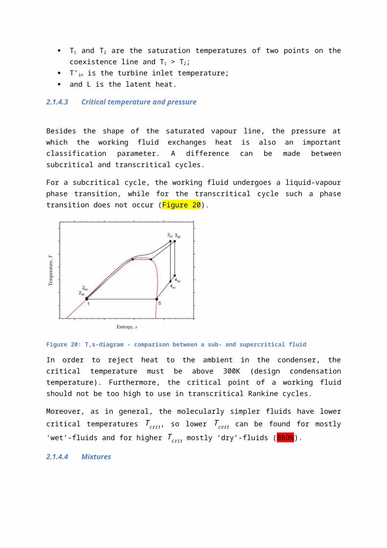
I=T 0σ

Eq…⇒

I=T 0[ΔS−∫2

1

( δQT )b]

Eq…⇒

I=T 0[m ( s2−s1 )−Q k

T k ]The irreversibility of the pump is defined as:

I pump= ( E1+W pump )−E2

or

I pump=T0 mORC ( s2−s1 )

The irreversibility of the vapour generator is defined as:

I vap−gen=( Einlet ,WH+ E2 )−( Eoutlet ,WH+ E3 )

With Eq…. and dQ=dH (isobar process), the irreversibility can be written as:

I vap−gen=T 0mORC [ (s3−s2 )−h3−h2TWH ]

The irreversibility of the expander is defined as:

I exp=E3−(W exp+ E4 )

or

I exp=T 0 mORC (s4−s3 )

The irreversibility of the condenser is defined as:

I cond=E4−E1

With Eq…. and dQ=dH (isobar process)

I cond=T 0 mORC [ ( s1−s4 )−h1−h4T CS

]The irreversibility of the IHE is defined as:

I IHE=( E4+ E2 )−( E4a+ E2a )

or

I IHE=T 0mORC [ ( s4a+s2a )−( s4+s2) ]

The irreversibility of a process, I tot, is the sum of all of available exergy destruction of all the streams in the system:

I tot=∑jI j= I pump+ I vap−gen+ I exp+ I cond+( I IHE)

The major exergy destruction in the vapour generator or the condenser is due to heat transfer over a finite temperature difference, and the exergy destruction in the turbine or pump is due to the friction losses of the flow through the turbine or the pump, the non-ideal adiabatic expansion or compression in the turbine or the pump, and the corresponding irreversibilities.

As the heat source is not cooled down to the dead state temperature T 0, the rest of exergy after the heat exchanger that is not used, is regarded as losses. Figure 23 [23]shows the hatched exergy destruction due to heat transfer and losses (exergy transportation to the environment) due to incomplete cooling down of the heat source for sub- and supercritical conditions.

Figure 23: Exergy losses and destruction in subcritical (left) and supercritical (right) heating process.

2.2.1.2.2 Exergy destruction factor (EDF)

The exergy destruction factor of a component can be defined as the ratio of the exergy destruction of the component to the net power produced by the cycle (bron).

EDFcomponent=I component

W net

2.2.1.3 Other efficiencies

Some authors use also other efficiencies to express the performance of the power cycle, but these are less used because the external exergy efficiency and utilisation efficiency already give a very good representation of the performance of the cycle.

2.2.1.3.1 Heat-exchanger and system efficiency [10] [23]

One of the main goals of an optimal working organic Rankine cycle is not to have the maximum thermal efficiency, but to maximize the power output from a given heat source.

The efficiency of the heat exchanger, which transfers the heat from the waste heat source to the organic fluid, is defined as:

ηHX=QOrganic fluid

QWH

The efficiency of the whole system then can be defined as:

ηSystem=Pmech

QWH=ηthηHX

As the efficiency of the ORC system is directly linked with the efficiency of the heat-exchanger, it is our goal to maximize the transferred heat.

Schuster and Karellas (2008) [10] performed simulations with subcritical and supercritical fluid parameters for applications of waste heat recovery from internal combustion engines and a geothermal power plant. Using R245fa as working fluid for the waste heat recovery from IC engines (thermal oil at 240°C); a 13% higher system efficiency was found in the case of supercritical fluid parameters.

2.2.1.3.2 Recovery efficiency [65]

The thermal efficiency represents the ORC itself, neglecting the thermal behaviour of heat sources and sinks. The recovery efficiency takes this influence into consideration and is a more meaningful parameter.

ηr=net work

potential energy of waste heat=

W net

Wmax

With Wmax is the maximum theoretical power produced by a Carnot engine operating between the heat source inlet temperature and the ambient temperature.

Wmax=mWH c p ,WH (T ¿ ,WH−T0)(1−T0

T ¿ ,WH)

Net power output of the system can be given:

W net=W exp−W pump−W pump ,CS (−W pump ,WH )

W pump ,WH=mWH ΔpwH

ρWH ηpump,WH

W pump ,CS=mCS ΔpCS

ρWCSηpump ,CS

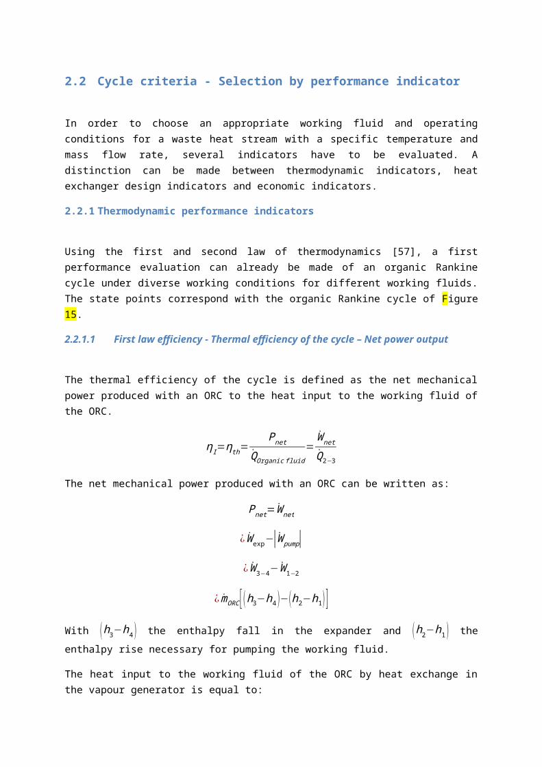
2.2.1.3.3 Rankine cycle efficiency (bron)

The Rankine cycle efficiency is defined as:

ηRankine=Q vap−gen−Qcond

Qvap− gen

With:

Heat supply in vapour generator:

Qvap−gen=mORC (h3−h2)

Heat rejection in the condenser:

Qcond=mORC (h4−h1)

2.2.2 Heat exchanger performance indicators

Besides the thermal and exergy efficiency and net power output, another objective for optimization can be the performance indicators related to the heat exchangers used in the cycle.

The two objective functions considered in literature are the heat transfer capacity and the total heat exchanger area.

2.2.2.1 Heat transfer capacity UA capacity

Schuster et al. [23] uses the heat transfer capacity in his research to investigate the influence of the maximum cycle temperature (turbine inlet temperature) on UA for a selection of working fluids. It has to be noted that good system efficiencies and low exergy losses are not directly followed by low values for the heat transfer capacity UA [23]. This indicates again the importance of a good choice of the objective function.

Cayer et al. [62] [66] uses the heat transfer capacity as an objective function and checks the influence of the turbine inlet temperature, turbine inlet pressure and the net work output on the value of UA for a transcritical cycle using CO2, ethane and R125.

The general results can be found in Chapter 7 Fluid selection and cycle optimization.

A better objective function as heat exchange performance indicator can be the minimization of the total area needed for heat exchange. A low value for UA can indicate on a small heat exchange surface, which is positive, but it can also indicate on a low overall heat transfer coefficient.

2.2.2.2 Total heat exchanger surface

Cayer et al. [62] [66] also investigated the influence of the turbine inlet temperature, turbine inlet pressure and the net work output on the value of UA for a transcritical cycle using CO 2, ethane and R125.

The general results can be found in Chapter 7 Fluid selection and cycle optimization.

The gap between two consecutive points of the temperature profiles of the heat source and sink with the working fluid say something about the heat transfer rate and consequently the heat transfer surface.

Figure 24: Optimized carbon dioxide transcritical cycle (left) and optimized R125 transcritical cycle (right).

A wide gap indicates that the segment has a high heat transfer rate compared with points having a narrow gap.

In the case of the carbon dioxide in the vapour generator (Figure 24), the segments near the exit have relatively low heat transfer rates due to the low temperature difference. In contrast, a larger heat transfer area is occupied by the middle range of the R125 vapour generator.

2.2.2.3 Heat exchanger efficiency

For the calculation of the heat exchanger efficiency, the -NTU method cannot be used, as in some parts of the heat transfer procedure, neither the temperature nor the specific heat capacity are constant. In a subcritical heat transfer process one of the two values is constant. In the sensible heat transfer procedures, c p is considered constant, where in latent heat transfer procedures (evaporation) the temperature remains constant. Therefore, the following definition was used for the efficiency of the heat exchanger [67]:

ε= QQmax

With Q the heat transferred to the organic working fluid and Qmax the maximum transferable heat, defined as:

Qmax=Cmin¿

Cmin=min {(m c p )WH , (m c p )ORC }

2.2.3 Cost performance indicators

A complete economic analysis is rather complex, because it is dependent on several parameters which are influenced by future local and global events.

Zhang S. et al. [65] and Cayer et al. [66] were one of the first who performed a thermo-economic parameter analysis for a selection of working fluids in transcritical organic Rankine cycles (R134a, R143a, R218, R125, R41, R170, ethane and CO2).

The general results can be found in Chapter 7 Fluid selection and cycle optimization.

Cayer et al. [66] uses well-estimated purchase prices for the major components of the cycle (pump, turbine and heat exchangers) as the representative of the complete life cycle cost, even if it is just a fraction of the actual total cost.

Zhang S et al. [65] considers the total cost of the heat exchangers representative of the complete system cost of an ORC, because 80-90% of the system capital cost can be assigned on the heat exchangers [68] [69] [70].

Two economic performance indicators can be used for evaluation of a power system:

APR LEC

2.2.3.1 APR

As it is stated that the total cost of a heat exchanger is representative for the complete system cost [68] [69] [70], the APR can be used as a performance indicator for evaluation of an organic Rankine cycle.

APR is the ratio of the total heat transfer area to the total net power output [69].

APR=A tot

W net

The result of the APR doesn’t give an economical value, but it says something about the heat exchange area needed for a certain amount of net power output. The goal is to minimize this function to obtain as much power with as less heat exchange surface.

2.2.3.2 Levelized energy cost LEC

The levelized energy cost is defined as the ratio of the system cost to the total net power output [70].

The purchase price of the components can be calculated by the following general correlation [71]:

log10Cb=K1+K2 log10Z+K 3 ( log10Z )2

With:

Cb the basic cost of the equipment assuming ambient operating pressure and carbon steel

construction in the year of 1996 (US dollar). Z is a dimensional parameter which corresponds to the total area in m2 for the heat

exchangers, the power output in kW for the turbine and the power input in kW for the pump. K1 ,K 2 and K3are component and material specific coefficients.

Cayer et al. [66] chose the following specifications for his case:

an axial gas turbine in cast steel; an electric centrifugal pump in cast steel; a fixed head shell and tube vapour generator in cast steel; and a fixed head shell and tube condenser in stainless steel.

Zhang S et al. [65] chose:

a fixed head shell and tube vapour generator in cast steel; a fixed head shell and tube condenser in stainless steel; and the operating pressure of both heat exchanger are much higher than the ambient

pressure.

This basic cost then has to be corrected for the chosen material and for the working pressures by following correlation:

log10 Fb=C1+C2 log10P+C3 ( log10P )2

The corrected cost CBM than be defined as:

CB M=Cb (B1+B2FM Fb )

With:

FM the material correction factor;

Fb the pressure correction factor;

and B1 and B2 the coefficients characterising each type of equipment.

The total CBM is calculated by summating the CBM of each component.

The cost of the power plant also needs to be converted from the costs in 1996 to the present day by using Chemical Engineering Plant Cost Index (CEPCI) values, which are published in the Chemical Engineering Journal and allows adjusting process plant construction costs from one period to another [71].

CC pl , present=CC pl, 1996

CEPCI present

CEPCI 1996

All the coefficients (K i, C i, FM , Fb and CEPCI i) are available in literature [72].

Taking into account the interest rate (i, e.g. 5%) and the lifetime of the plant (¿, e.g. 20 years), the capital recovery cost can be defined [73]:

CFR=i (1+i )¿

(1+ i )¿−1

The levelized energy cost then can be calculated by [70]:

LEC=CFRxCC pl , present+COM pl

AE

Where:

CC pl , present is the present capital cost of the power plant in US dollar;

COM pl the operations and maintenance cost of the power plant US dollar (e.g. 1.5% of CC pl

); AE the annual net power output of the power plant in kW.

3. Working fluids for organic Rankine cycles

3.1 Fluid candidates

More than 50 working fluids have been suggested in the literature, among which some have been phased out as required by the protocols ( PAPER “PHASE OUT HAVE WE MET THE CHALLENGE”), and some are not practical for application due to their properties (e.g. methane). Based on the criteria of safety, environmental issues, critical temperature and availability, a list of pure working fluids that could be used in for organic Rankine cycles and transcritical Rankine cycles is presented in Table 4. Multi-component fluids are not completely included in this table, because the mixing rule is rather complicated and there are a lot of combinations possible.

Table 4: Overview of potential working fluids for ORCs

Physical data Safety data Environmental data

Name Type Tcrit (°C)pcrit

(bar)ASHRAE 34

safety groupATL (yr) ODP

GWP (100 yr)

R-116 19,88 30,50 0 11900R-23 26,14 48,30 0 n.a.R-747 - CO2 WET 31,10 73,80 A1 >50 0 1R-170 WET 32,18 48,00 A3 0,21 0 ~20R-41 WET 44,13 59,00 n.a. 2,4 0 92R-125 WET 66,02 36,20 A1 29 0 3500

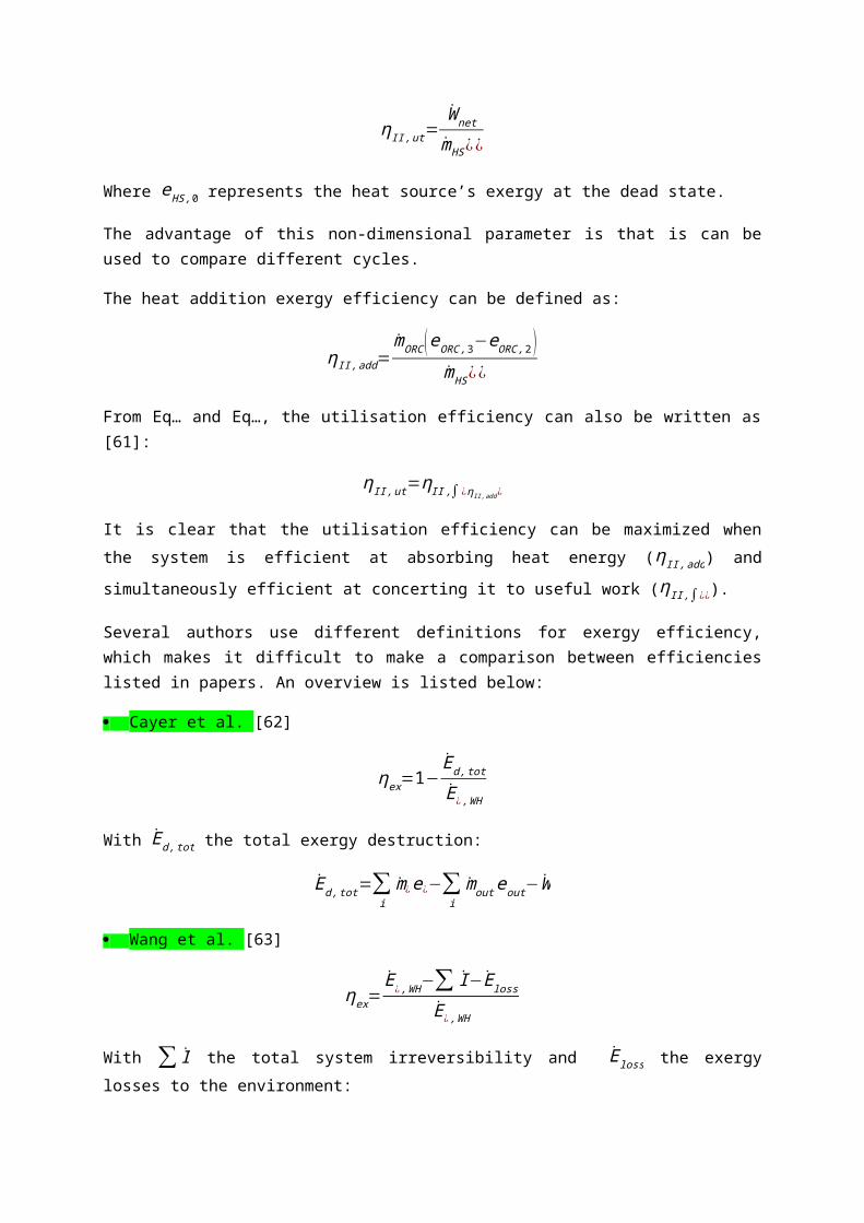
R-410A 70,20 47,90 A1 16,95 0 2088R-218 DRY 71,89 26,80 A1 2600 0 8830R-143a WET 72,73 37,64 A2 52 0 4470R-32 WET 78,11 57,83 A2 4,9 0 550R-E125 WET 81,34 33,51R-407C 86,79 45,97 A1 n.a. 0 1800R-1270 WET 92,42 46,65R-22 96,15 49,90 0,03 1700R-290 - propane WET 96,65 42,47 A3 0,041 0 ~20R-134a Isentropic 101,03 40,56 A1 14 0 1430R-227ea DRY 101,74 29,29 A1 42 0 3220

R-500 105,50 44,55 A1 n.a. 0,738 8100R-12 112,00 41,14 A1 100 1000 10890R-3-1-10 113,18 23,20 0 8600R-152a WET 113,50 44,95 A2 1,4 0 124R-C318 115,20 27,78 A1 3200 0 10250R-124 122,28 36,20 0,03 620CF3I WET 123,29 39,53R-C270 - cyclo-propane WET 124,65 54,90R-236fa DRY 125,55 32,00 A1 240 0 9810R-E170 WET 126,85 52,40R-717 - Ammonia 132,30 113,33 B2 0,01 0 <1R-E245mc DRY 133,68 28,87R-600a - iso-butane DRY 135,05 36,47 A3 0,019 0 ~20R-142b 137,11 40,60 0,04 2400R-236ea DRY 139,22 34,12 n.a. 8 0 1370R-114 145,70 32,89 A1 300 0 10040R-E134 DRY 147,10 42,28FC-4-1-12 147,41 20,50 0 9160C5F12 DRY 148,85 20,40R-600 - n-butane DRY 152,00 37,95 A3 0,018 0 ~20R-245fa Isentropic 154,05 36,40 B1 7,6 0 900R-338mccq DRY 158,80 27,26neo-C5H12 - neo-pentane DRY 160,65 32,00R-E347mcc DRY 164,55 24,76R-E245 DRY 170,88 30,48R-245ca DRY 174,42 39,25 A1 62 0 560R-21 178,33 51,80 0,01 210R-123 Isentropic 183,70 36,68 B1 1,3 0,02 120R-601a - iso-pentane DRY 187,75 33,86R-601 - n-pentane DRY 196,50 33,64 - 0,01 0 ~20R-11 Isentropic 197,96 44,08 A1 45 1 1400R-141b 204,20 42,49 n.a. 9,3 0,12 725R-113 214,10 34,39 A1 85 1000 6130n-hexane DRY 234,67 30,10Methanol 240,20 81,04 n.a. n.a. n.a. n.a.Ethanol Wet 240,80 61,48 n.a. n.a. n.a. n.a.Cyclo-hexane 280,50 40,75 A3 n.a. n.a. n.a.OMTS 290,85 14,40Toluene Dry 318,85 41,10R-718 - Water Wet 374,00 220,64 A1 n.a. 0 <1Benzene IsentropicHFE7100 Dryisobutenep-Xylene DryR-236faR-365mfc

Chen H. et al [48] made a distribution of 35 pure working fluids in a T ,ξ-diagram (Figure 25, Figure26), from which the critical temperature and the type of each working fluid is shown. The fluids are divided into 5 groups based on their locations in the T ,ξ-diagram.

Figure 25: Distribution of the screened 35 working fluids in T ,ξ -diagram

Figure 26: Close-up look of the distribution of the remaining 31 working fluids in T ,ξ -diagram

3.1.1 Group 1: Fluids ammonia, benzene and toluene

Water is located in the upper left of the chart, which indicates it is the wettest fluid and has the highest critical temperature among all the fluids plotted, which makes it unsuitable for low-

temperature heat conversion. Ammonia is a very wet fluid, which needs superheating when used in an organic Rankine cycle. Ammonia is not recommended in transcritical Rankine cycles, since the critical pressure is relatively high (11.33MPa). Benzene and toluene are considered as isentropic fluids with relatively high critical temperatures, which are desirable characteristics for organic Rankine cycles. Benzene and toluene are chemically stable in these potential operating conditions [9].

3.1.2 Group 2: Fluids R170, R744, R41, R23, R116, R32, R125 and R143a

Fluids R170, R744, R41, R23, R116, R32, R125 and R143a are wet fluids with low critical temperatures and reasonable critical pressures (Table …), which are desirable characteristics for transcritical Rankine cycles. Carbon dioxide (R744) and R134a have been studied in transcritical Rankine cycles in the literature. Among these fluids, R170, R744, R41, R23 and R116 have critical temperatures below 320 K, which require low condensing temperatures, not achievable under many circumstances. The critical temperatures of R32, R125 and R143a are above 320 K, so the design of condensers for these fluids is not a big concern. Provided other aspects are satisfied, R32, R125 and R143a could be promising working fluids for transcritical Rankine cycle.

3.1.3 Group 3: Fluids propyne, HC270, R152a, R22 and R1270

Propyne, HC270, R152a, R22 and R1270 are wet fluids with relatively high critical temperatures. Superheat is usually needed for this group of fluids when applied in organic Rankine cycles. They might be applied in transcritical Rankine cycles if the temperature profile of the heat source meets the requirements. However, propyne, HC270 (cyclopropane) and R1270 (propene) are not normally used in their supercritical state due to the stability concerns. Propyne, HC270 and R1270 have relatively low molecular weight (Table …). Applying these fluids implies a larger system size compared to those fluids with higher molecular weight.

3.1.4 Group 4: Fluids R21, R142b, R134a, R290, R141b, R123, R245ca, R245fa, R236ea, R124, R227ea, R218

This group of fluids can be considered isentropic fluids. They can be applied in organic Rankine cycle or transcritical Rankine cycle depending on the temperature profile of the heat source. Since the isentropic expansion would not cause wet fluid problems, superheat is not necessary in organic Rankine cycle with these fluids. Among these fluids, R141b, R123, R21, R245ca, R245fa, R236ea and R142b have critical temperature above 400 K, making them more likely to be used in organic Rankine cycle than in transcritical cycle for low-temperature heat sources, while the rest may be used in either cycle, depending on the heat source profile.

3.1.5 Group 5: Fluids R601, R600, R600a, FC-4-1-12, RC318, R-3-1-10

Fluids R601, R600, R600a, FC-4-1-12, RC318, R-3-1-10 are considered dry fluids. Based on the analysis before, dry fluids may be used in transcritical Rankine cycles and organic Rankine cycles. Since superheat has a negative effect on the cycle efficiency when dry fluids are used in organic

Rankine cycle, superheating is not recommended. The decision on which fluids could be used may be based on how the operating temperature is tailored to cope with the heat source temperature profile.

Later, these fluids will be evaluated on their thermodynamic performances, depending waste heat source.

3.2 Working fluids for transcritical organic Rankine cycles

In order to form a transcritical cycle, the critical temperature of the working fluid should be lower than the heat source temperature and higher than the condensing temperature. A part of the cycle will be located in the supercritical region.

Much research has already been done using carbon dioxide in transcritical power cycles (Chen H. et al. [47]; Chen Y. et al. [58]; Cayer E. et al. [62] [66]; Wang J. et al. [63]). This mainly due to the fact that CO2 has a low critical temperature (31.1°C), is compact, non-toxic, inexpensive, abundant in nature and environmental friendly. Recycling or recovery of CO2 would not be necessary, either for environmental or economic reasons. CO2 is also thermally stable and behaves inertly, thus eliminating material problems or chemical reactions in the system. A transcritical CO 2 power cycle shows a high potential to recover low-grade waste heat, because of the low critical temperature and the better temperature glide matching between the heat source and working fluid in the vapour generator. Transcritical CO2 also doesn’t have a pinch limitation in the vapour generator. Although, it should be noted that condensation of carbon dioxide can be difficult in some places because of its low critical temperature. Furthermore, an operating condition of 60-160 bar is a safety concern.

Research in the use of supercritical CO2 is mainly found in solar energy powered Rankine cycles, either for power generation, heat generation or a combined cycle of power and heat (Zhang X.R. et al.). Numerical simulations show that the proposed system may have an annual average power generation efficiency and heat recovery efficiency as high as 11.4% up to 20.0% and 36.2% up to 68.0%, respectively. The cycle efficiencies and outputs can be significantly increased by increasing the CO2 mass flow rate (Zhang X.R. et al. [32] [33]).

Furthermore, Zhang X.R. et al. designed and constructed an experimental prototype of a solar energy powered Rankine cycle using supercritical CO2. The system performance was evaluated based on daily, monthly and yearly experiment data. The experimental results show that CO2 works stable in the transcritical region and the estimated power generation efficiency is 8.78%-9.45% and heat recovery efficiency is 65.0%-70.0% [42] [64]. Supercritical CO2 actually has physical properties somewhere between those of a liquid and a gas. So it is difficult to decide whether a turbine of a gas or a liquid type should be used for the Rankine cycle using supercritical CO2. Therefore, in the prototype, a throttling valve was used, instead of a turbine, in order to study the cycle performance. The throttling valve can provide various extents of opening for the cycle loop in order to simulate pressure drop occurring in realistic turbine condition and consequently a thermodynamic cycle can be achieved.

INSERT MORE REFERENCES WITH TRANSCRITICAL CYCLES FROM EXCEL FILE WITH RESEARCH OVERVIEW

Besides CO2, also organic fluids like isobutene, propane, propylene, difluoromethane and R245fa (Schuster et al. [10]) have been suggested for transcritical Rankine cycles. It was found that supercritical fluids can maximize the efficiency of the system (Schuster et al. [10]).

Not only pure substances show a better performance in a transcritical cycle, but also mixtures can be used. Chen H. et al [47] [56] made a comparative study between a subcritical ORC with R134a and a transcritical ORC with a zeotropic mixture of R134a and R32 (0.7R134a/0.3R32). Due to the better thermal match during heating and condensing, an overall better performance for the transcritical working zeotropic mixture (thermal efficiency, net work output and exergy efficiency) was accomplished. An improvement of 10% to 30% in thermal efficiency was found for Tmax-range between 120 and 200°C and the exergy efficiency improved about 60% compared to the subcritical cycle. At Tmax 200°C the transcritical ORC provides 38.9% more net work compared to the subcritical ORC.

Table 5 shows an overview of the working fluids that can be used in transcritical cycles, according to the temperature range of the waste heat stream.

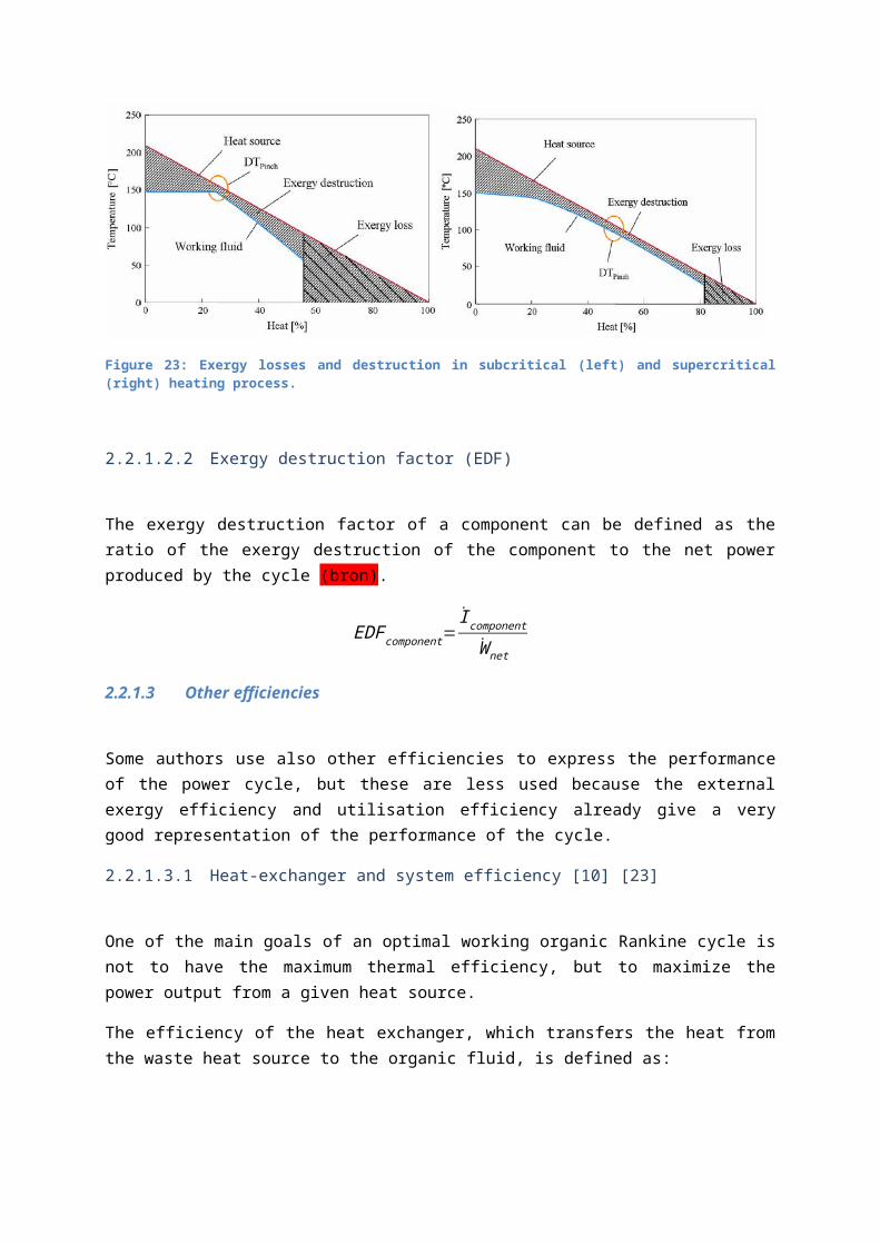
Table 5: Overview of potential working fluids for transcritical ORCs

Physical data Safety data Environmental data

Name Type Tcrit (°C)pcrit

(bar)Molecular

weight (g/mol)ASHRAE 34

safety groupATL (yr) ODP

GWP (100 yr)

PFC-116 Wet 19,88 30,50 138,02 A1 10000 0 11900

HFC-23 Wet 26,14 48,30 70,01 A1 270 0 14800

R-744 (CO2) Wet 31,10 73,80 44,01 A1 >50 0 1

HC-170 (ethane) Wet 32,18 48,00 8,70 A3 0,21 0 ~20

HFC-41 Wet 44,13 59,00 34,03 Flammable 2,4 0 92

HFC-125 Wet 66,02 36,20 120,02 A1 29 0 3500

HFC-410A - 70,20 47,90 72,58 A1 16,95 0 2088

PFC-218Isentropi

c 71,89 26,80 188,02 A1 2600 0 8830

HFC-143a Wet 72,73 37,64 84,04 A2 52 0 4470

HFC-32 Wet 78,11 57,83 52,02 A2 4,9 0 550

HFC-407C - 86,79 45,97 86,20 A1 15657 0 1800

HC-290 (propane) Wet 96,65 42,47 44,10 A3 0,041 0 ~20

HFC-134aIsentropi

c 101,03 40,56 102,03 A1 14 0 1430

HFC-227ea Dry 101,74 29,29 170,03 A1 34,2 0 3220

PFC-3-1-10 Dry 113,18 23,20 238,03 - 2600 0 8600

HFC-152a WET 113,50 44,95 66,05 A2 1,4 0 124

PFC-C318 Dry 115,20 27,78 200,03 A1 3200 0 10250

HCFC-124Isentropi

c 122,28 36,20 136,47 A1 5,8 0,03 620

HC-600a (isobutane) DRY 135,05 36,47 58,12 A3 0,019 0 ~20

HCHF-142bIsentropi

c 137,11 40,60 100,49 A2 17,9 0,04 2400

HFC-236ea Dry 139,22 34,12 152,04 - 10,7 0 1370

PFC-4-1-12 Dry 147,41 20,50 288,03 - 4100 0 9160

HC-600 (n-butane) Dry 152,00 37,95 58,12 A3 0,018 0 ~20

HFC-245faIsentropi

c 154,05 36,40 134,05 B1 7,6 0 900

HFC-245ca Dry 174,42 39,25 134,05 A1 6,2 0 693

HCFC-21 Wet 178,33 51,80 102,92 B1 1,7 0,01 210

HCFC-123Isentropi

c 183,70 36,68 152,93 B1 1,3 0,02 77

HC-601 (n-pentane) Dry 196,50 33,64 72,15 A3 0,01 0 ~20

HCFC-141bIsentropi

c 204,20 42,49 116,95 A2 9,3 0,12 725

Chapter 5Modelling

1. Introduction

The first step towards a fundamental understanding and estimation of the performance and characteristics of the system is a mathematical model that simulates the behaviour of the Rankine cycle.

To define the thermodynamic state of each point, the energy balances will be made. With these balances, the first conclusions can already be made concerning efficiency and power output. Because our interest is in the heat transfer from the waste heat source to the supercritical working fluid, a second step in the analysis is the heat transfer modelling. Here the heat exchangers will be discretized, due to the variable properties of the supercritical fluid during heating. To determine the local heat transfer in each section, experimental correlations will be used for the heat transfer coefficients.

In most of the research done, friction and the pressure drop are neglected. Baik et al. [59] and Zhang S. et al. [65] were the first who took the pressure drop in the system into account.

Besides the thermodynamic modelling, an economic analysis will be done using the cost performance indicators mentioned in Chapter 4 section 2.2.3.

2. Energy balances

The energy balance is made for all the components in the ORC system: the pump, the vapour generator, the expander, the condenser and if necessary the regenerator or internal heat exchanger.

Figure 27: ORC with IHE (regenerator) and T,s-diagram

3.3 Pump

To bring the working fluid from the condensing pressure to the pressure present in the vapour generator, a feed pump is required. The required work is W 1−2.

W 1−2=mORC (h2−h1) /ηmech, pump

W 1−2=mORC (h2 s−h1 )/(ηs , pump η¿¿mech , pump)¿

With ηs , pumpthe isentropic efficiency of the pump, which is defined as:

η s , pump=h2 s−h1h2−h1

ηmech , pump is the mechanical efficiency of the pump.

3.4 Vapour generator

Between state point 2 and 3, there is heat exchanged between the working fluid and the waste heat source. The added heat to the working fluid is Q2−3.

Q2−3 .=mORC (h3−h2 )

3.5 Expander

During the following expansion process work is delivered in the expander. The delivered power W 3−4 is given by:

W 3−4=mORC (h3−h4 )ηmech, exp

The maximum temperature in the cycle occurs at the expander inlet.

The isentropic efficiency of the expander is defined as:

ηs ,exp=h3−h4h3−h4 s

The volume flow rate of the working fluid at the expander inlet and outlet are defined as:

V 3=mORC υ3

V 4=mORCυ4

The vapour expansion ratio VER of the expander is defined as:

VER=υ4 /υ3

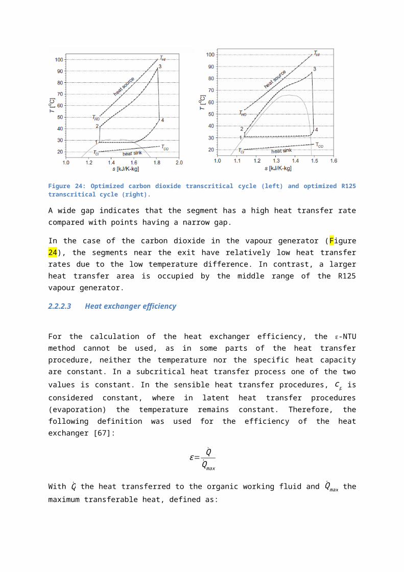
3.6 Condenser

The excess heat flow rate Q4−1 is then removed in the condenser during process (4-1) and is defined as:

Q4−1=mORC (h4−h1)

The minimum temperature in the cycle occurs at the condenser outlet.

3.7 Regenerator (Internal Heat Exchanger)

In case that the endpoint of the expander (state point 4) is located in the superheated vapour region, the temperature T 4 will be higher than the temperature T 2. If this temperature difference is remarkable, it could be interesting [74] to add an extra internal heat exchanger (IHE or regenerator) to the cycle. But, as an internal heat exchanger increases the cycle efficiency, recent studies have shown that it has little influence on the net power output and significantly increases the heat exchange surface and consequently the cost [62] [65]. 

This heat exchange is presented in the cycles by state point 4a and 2a. The saturated vapour cools down in the internal heat exchanger in the process (4–4a) by transferring the heat q4−4 a to the already compressed liquid which is heated up in the process (2–2a) by the heat q2−2a.

Due to the variable specific heat of a supercritical fluid near the critical temperature, the traditional definition of the effectiveness cannot be used, because this assumes a constant value for the specific heat. Instead of considering a constant specific heat and working with the temperature differences as in the traditional approach, the enthalpy difference is used to express the effectiveness.

The heat exchanged between the two streams in the regenerator is:

Q2a−2=Q4−4a=mORC (h2a−h2 )=mORC (h¿¿ 4−h4 a)¿

In an ideal heat exchanger, one of the following two situations can occur depending on which of the two streams in the regenerator has the smaller heat capacity: either T 4a tends towards T2 or T2a tends towards T4. In this way, the maximum heat exchange Qmax is given by the smaller of the following two quantities:

¿

The regenerator effectiveness IHX is then expressed as:

ε IHE=mORC (h4−h4 a )

Qmax=

mORC (h2a−h2 )Qmax

The use of variable properties in the regenerator by applying Eq. …, … and … instead of the traditional ones obtained by replacing the enthalpy differences by the product of temperature differences and a constant specific heat, has a very significant effect on the cycle thermal efficiency. For example, for a

transcritical CO2-cycle [62] with a high pressure of 7.5 MPa and maximum and minimum cycle temperatures of 95°C and 15°C, respectively, the thermal efficiency obtained with the traditional method is 25.8% versus 6.3% when considering variable properties. Since the corresponding Carnot efficiency is 21.7%, it is obvious that the traditional definition of the effectiveness leads to unacceptable results. By extension, the LMTD and –NTU methods, which are also based on the assumption of constant properties, should not be used in transcritical analyses.

3. Heat transfer

A widely used method of calculating the heat transfer capacity UA is by applying the logarithmic mean temperature difference (LMTD) between the inlet and outlet of the heat exchanger.

Q=U . A . ΔT log=U . A .ΔT 1−ΔT 2

ln( ΔT 1ΔT 2 )

However, the LMTD-method is based on constant properties, an assumption leading to incorrect results in the case of supercritical fluids. An alternative solution consists in discretizing the heat exchangers so that the properties variation in each step is small and an average constant value, different for each step, can be assigned to each of them. The discretization is performed by dividing the overall enthalpy change for one of the streams in N equal differences h (Cayer et al. [62]). Without partitioning, the calculation error will be unacceptable [67].

Figure 28 presents the heat transfer between the heat source and the supercritical organic working fluid.

Figure 28: Q,T-diagram of a supercritical heat exchange process.

By discretizing the heat exchanger, assuming a counter-flow configuration, the heat transfer for each step i and the fractional heat transfer capacity UAi are calculated with the following equations:

{QORC ,i ;i+1=mORC (hORC ,i+1−hORC ,i )QHS ,i ;i+1=mHS (hHS ,i−hHS, i+1 )

¿ mHS c p (T HS,i−T HS ,i+1)

Heat flow of the heat source is supposed to be linear. A dependence of the heat capacity with the temperature is not considered.

Qi ;i+1=UAi ;i+1 .ΔT i−ΔT i+1

ln( ΔT i

ΔT i+1 )With

¿

The overall heat transfer coefficient for a tube with inner diameter d in and outer diameter dout, calculated on the inner diameter is defined by:

1U ¿ A¿

= 1A¿h¿

+ln( dout

d¿)

2π λwL+ 1Aouthout

❑⇒

1U ¿

= 1h¿

+A¿ ln ( dout

d¿)

2π λwL+ A¿

Aouthout

With

{ A¿=π d¿ LAout=π dout L

Implemented on a discretized section, the sectional overall heat transfer coefficient calculated on the inner diameter, U ¿ ,i ;i+1, can be written as:

1U ¿, i; i+1 A ¿ ,i ;i+1

= 1A¿,i ;i+1h¿ ,i ; i+1

+ln( dout

d¿)

2π λw Li ;i+1+ 1Aout ,i ;i+1hout , i; i+1

❑⇒

1U ¿ ,i ;i+1

= 1h¿ ,i ;i+1

+d¿ ln (dout

d¿)

2 λw+

d¿

dout

hout ,i ;i+1

To calculate the sectional overall heat transfer coefficient, the local heat transfer coefficients need to be known. In the following section, several correlations are given for the local convection heat transfer coefficients.

Once the sectional overall eat transfer coefficient U ¿ ,i ; i+1 is calculated, then the corresponding surface A¿ ,i ;i+1 (or equivalent length Li ;i+1) can be calculated.

The total surface A of the heat exchangers can be calculated by adding the surfaces of all individual sections Ai ; i+1.

3.1 Vapour generator

3.1.1 Working fluid – heat transfer coefficient

The correlations for the convection heat transfer coefficient of the supercritical working fluid are discussed in the literature study about supercritical heat transfer. Here an overview is given of the correlations used in research for transcritical organic Rankine cycles.

The classical heat transfer correlations for the calculation of the Nusselt number cannot be used due to the variations around the critical point. Krasnoshchekov and Protopopov (1966) and Jackson et al [75] [76] developed in correlations for supercritical fluid parameters. The correlations have a correction factor which neutralizes the effect of the variations of the thermo-physical properties around the pseudo-critical point and provides more stable and accurate results.

Baik et al. [59] use a Nusselt-correlation proposed by Krasnoshchekov and Protopopov (1966) in [77] for carbon dioxide in the supercritical range at high temperature drops, which take the difference is properties between the wall and the bulk into account.

Nub=Nu0 , b( ρw

ρb)0.3

( c p

c p ,b)n

Where b refers to the bulk fluid temperature and w to the wall temperature.

Nu0 ,b is calculated using the Petukhov-Kirillov correlation [78] (1958) and the bulk temperature of the fluid. The average specific heat c p is defined as:

c p=hb−hw

T b−T w

The exponent n is expressed as a function of the pseudo-critical T pc, wall T w and bulk temperature T b of the fluid [77].

Cayer et al. [62] [66], Song Y et al. [79] and Zhang S. et al. [65] also use the correlation of Krasnoshchekov, Protopopov and Petukhov [80] in a slightly different form.

Nub=Nu0 , b( c p

cp ,b)0.35

( λb

λw)−0.33

( μb

μw)−0.11

With

Nu0 ,b=(f b8

ℜb Pr

12.7( f b8 )0.5(Pr

23−1)+1.07 )

Where the Darcy friction factor is expressed as

f=(1.82 log10 (ℜb )−1.64 )−2

Schuster and Karellas [81] use the Jackson correlation [82] (1979):

Nub=0.0183ℜb0.82Pr0.5( ρw

ρb)0.3

( c p

c pb)n

The exponent n of the equation is defined as follows [83]:

For: T b<T w<T pc∧1.2T pc<Tb<T w

n=0.4

For: T b<T pc<T w

n=0.4+0.2( T w

T pc−1)

For: T pc<T b<1.2T pc

n=0.4+0.2( T w

T pc−1)(1−5( T b

T pc−1))

3.1.2 Heat source

Several researchers use different correlations to determine the convective heat transfer on the hot side. An overview is given below.

Cayer et al. [62] [66] use the Petukhov correlation [84] to calculate the convection heat transfer coefficient on the hot side using hot air as heat source.

U g=k g

D [ f g

8ℜg Prg

12.7( f g

8 )0.5(Prg

23−1)+1.07 ]

It is to be noted that the equivalent diameter of the shell must be used in this equation and that the air flow is supposed parallel to the tubes.

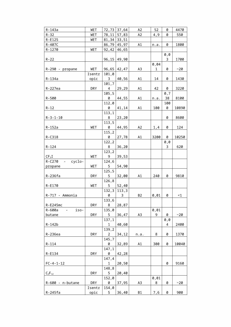
Zhang S. et al. [65] use hot water as heat source and the following correlation for the convection heat transfer coefficient:

hw=j0Gwc p , w

Prw23

( μμw )

0.14

Schuster and Karellas [81] and Song Y et al. [79]using the Dittus-Boelter correlation from [84]:

Nu=0.023 Prnℜ0.8

With n=0.3 for cooling of the heat source.

Baik et al. [59] use the Gnielinski correlation for turbulent flow in tubes [84] for the calculation of the convection heat transfer coefficient on the heat side.

NuD=( f8 ) (ℜD−1000 )Pr

1+12.7 ( f8 )12 (Pr

23−1)

Where f is the Darcy friction factor that can be obtained from the Moody chart or for smooth tubes from the correlation by Petukhov [84].

f=(1.82 log10 (ℜb )−1.64 )−2

The Gnielinski correlation is valid for [84]:

0.5≤Pr ≤20003000<ℜn<5.106

3.2 Condenser

The condenser requires a more detailed analysis for the calculation of the UA value. As mentioned before, two situations are conceivable depending on the state of the working fluid at the turbine outlet. First, when the working fluid is at a superheated vapour state, the condenser is divided into a single-phase region and a two-phase region. Each region is then subdivided in a number of steps with equal enthalpy differences for the working fluid. Second, when the state of the working fluid at the exit of the turbine falls in the two-phase region, this region is subdivided in a sufficient number of steps with equal enthalpy differences and the first one ignored (Cayer et al. [62]).

3.2.1 Working fluid

3.2.1.1 Single-phase heat transfer coefficient

Baik et al. [59] use the Gnielinski correlation for turbulent flow in tubes [84] for the calculation of the convection heat transfer coefficient of the single-phase working fluid in the condenser.

NuD=( f8 ) (ℜD−1000 )Pr

1+12.7 ( f8 )12 (Pr

23−1)

Where f is the Darcy friction factor that can be obtained from the Moody chart or for smooth tubes from the correlation by Petukhov [84].

f=(0.79l n (ℜd )−1.64 )−2

The Gnielinski correlation is valid for [84]:

0.5≤Pr ≤20003000<ℜn<5.106

Cayer et al. [62] [66] use the Petukhov correlation [84] to calculate the convection heat transfer coefficient of the single-phase working fluid in the condensing stage.

U g=k g

D [ f g

8ℜgPr g

12.7( f g

8 )0.5(Prg

23−1)+1.07 ]

It is to be noted that the equivalent diameter of the shell must be used in this equation and that the air flow is supposed parallel to the tubes.

3.2.1.2 Two-phase heat transfer coefficient

If the expansion in the turbine or expander ends in the two-phase region, the most common used correlation by researchers (Cayer et al. [62] [66], Zhang S. et al. [65], Song Y [79]) for the convection heat transfer coefficient is the Cavallini and Zecchin correlation [85].

U=0.05ℜeq0.8 Prsat liq

0.33 k sat liq

D

Where the equivalent Reynolds number is defined as:

ℜeq=ℜvap( μsat vap

μsat liq)( ρsat liq

ρsta vap)0.5

+ℜliq

ℜliq=mf

A f(1−x )

Dw

μsatliq

ℜvap=mf

A fx

Dw

μsat vap

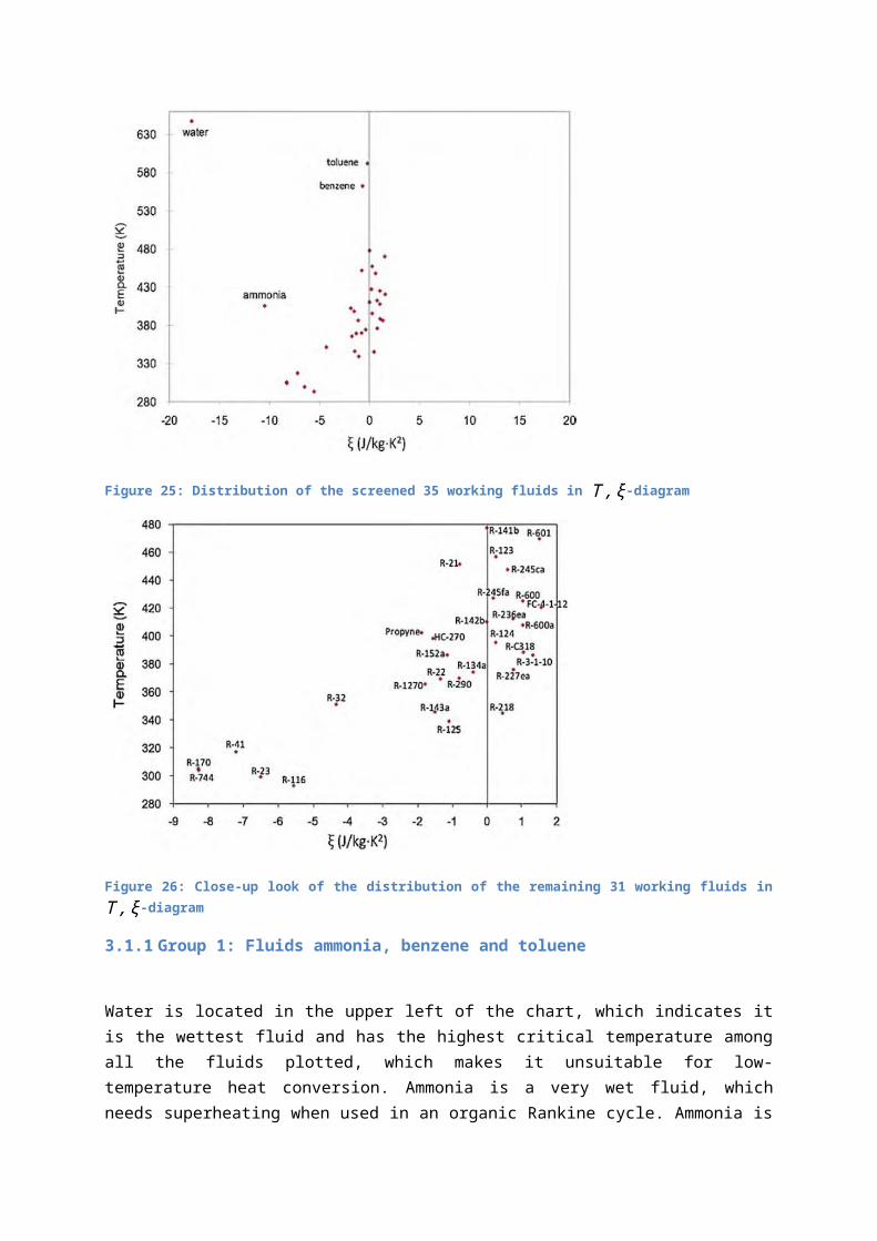
Baik et al. [59] uses the general correlation for heat transfer during film condensation inside pipes by Shah [86].

3.2.2 Cooling fluid

For the calculation of the convection heat transfer of the cooling fluid Baik et al. [59] use the Gnielinski correlation for turbulent flow in tubes [84], where all water properties are assumed to be a function of temperature only. Cayer et al. [62] [66] use the Petukhov correlation [84] and Zhang S. et al. [65] the Cavallini and Zecchin correlation [85].

3.3 Evaporator (subcritical)

In case a comparison is made between a subcritical and transcritical cycle, the correlations for the calculation of the convection heat transfer coefficient of the single-phase and two-phase region are given below.

3.3.1 Working fluid single-phase heat transfer coefficient

Zhang S. et al. [65] use the normal Dittus-Boelter correlation for single-phase heat transfer [85].

3.3.2 Working fluid two-phase heat transfer coefficient

For the two-phase region Zhang S. et al. [65] use the Wang-Touber correlation [87].

α tp={ αww0≤ x≤0.85

αww∨x=0.85−( x−0.850.15 )2

(αww∨ x=0.85−α ν ,all )0.85≤ x≤1

αww=3.4( 1X tt )0.45

α1 ,all

X tt=√(1−xx )

1.75( ν1ν ν)( μ1μν

)4. Pressure drop

4.1 Vapour generator

4.1.1 Working fluid

Baik et al. [59] uses the following equation for the pressure drop in the vapour generator:

Δ p=f G2ΔL2 ρ di

where the friction factor f is calculated by using the Blasius correlation, which works well for supercritical frictional pressure drop of carbon dioxide [88].

Zhang S. et al. [65] calculate the friction factor using the Kang correlation [89]:

f=0.316ℜ−0.25 for ℜ≤2x 104

f=0.184ℜ−0.20 for ℜ>2x 104

4.2 Condenser

4.2.1 Working fluid

4.2.1.1 Single-phase pressure drop

4.2.1.2 Two-phase pressure drop

Baik et al. [59] formulates the two-phase pressure drop in terms of the frictional effect and the acceleration effect only, neglecting the gravitational effect.

(Δ p )Ci =(Δ pF )C

i +( Δ pa )Ci

The frictional pressure drop Δ pF is calculated by the Müller-Steinhagen and Heck correlation [90] and the acceleration pressure drop Δ pa is expressed in terms of the qualities, void fractions, and specific volumes of the vapour and the liquid in their saturated states [91].

Zhang S. et al. [65] use the Kedzierski correlation [92].

Δ p=f G2( 1ρout+1ρ¿

) LDh

+G2( 1ρout−1ρ¿

)f=[0.002275+0.00933 e h

−0.003dr ]ℜB[ (x¿−xout )hLG

Lg ]0.211

ℜ=Gdh

μL

B=(−4.16−532 hdr )

−1

4.2.2 Cooling fluid - single-phase pressure drop

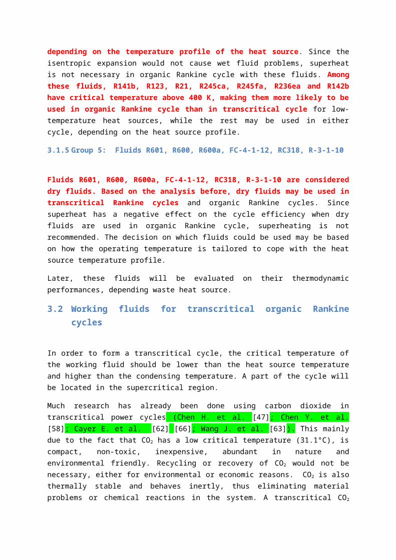
For the pressure drop in the cooling fluid of the condenser, Zhang S. et al. [65] use also the Kedzierski correlation [92].

4.3 Evaporator (subcritical)

In case a comparison is made between a subcritical and transcritical cycle, the correlations for the calculation of the pressure drop of the single-phase and two-phase region are given below.

4.3.1.1 Single-phase pressure drop

Zhang S. et al. [65] use the Wang-Touber correlation for single-phase pressure drop [87].

Δ ps=0.5 ρg ξ sΔ zus2/d

The friction factor ξ s is:

ξ s={ 64ℜ ( ℜ<2320 )

0.316ℜ−0.25 (2320≤ ℜ<8.104 )0.0054+0.3964ℜ−0.3(ℜ>8.104)

4.3.1.2 Two-phase pressure drop

Zhang S. et al. [65] use also the Wang-Touber correlation for the two-phase pressure drop [87].

Δ ptp=(ξm+x2−x1xm

+N b

2ξb

dL )( MA )

2 Lρmd

x1, x2 and xm are the entering, leaving and average vapour quality respectively.

ξm=0.053( ℜl

K f )0.25

ρm=1

xm

ρv+

(1−xm )ρl

ξb=ξom+ξ fm

ξom=1.2

ξ fm=2ξm

Lb

d

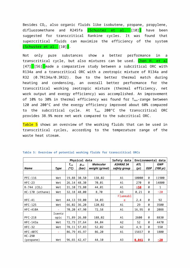
Chapter 6Fluid selection and cycle optimization

1. Parametric study and cycle optimization

To adequately compare different working fluids, parametric studies, optimization of the cycle parameters and a proper choice of the objective functions are required.

A parametric analysis is performed to evaluate the effects of each key parameter on the transcritical power cycle, such as turbine inlet pressure and temperature.

HERE THE FLOW CHART HAS TO COME AND BE DESCRIBED

Most studies done on transcritical cycles were limited to applying the first law of thermodynamics. A more detailed approach was necessary and Cayer et al. (2009) [62] presented a methodology using 4 performance indicators to analyse a transcritical CO2 power cycle using an industrial low-grade stream of process gases (100°C and a mass flow rate of 314.5kg/s). The used indicators were: the thermal and exergy efficiency, the total heat transfer capacity UA and the heat exchange surface. The variable parameters were the maximum cycle pressure (turbine inlet pressure) and the net power output. It was noticed that for each performance indicator, there was an optimum maximum cycle pressure, not necessarily all identical. Furthermore an augmentation of the net power output has no influence on the results of the energy analysis, but it decreases the exergy efficiency and increases the heat exchanger’s surface and has no significant effect on the optimizing maximum cycle pressure.

Cayer et al. [62] use a dimensionless parameter to compare the net power output of several cycles. Define as the fraction of the net power output to the maximum reversible power produced by a Carnot engine operating between the heat source and sink temperatures.

α=W net

Wmax

With: Wmax=mWH c p ,WH (T ¿,WH−T¿ ,CS)(1−T ¿ , CS

T ¿ , WH)

In the last term (Carnot efficiency) the temperatures are in K.

The mass flow rate of the organic working fluid can then be calculated as:

mORC=α Wmax

w

With w the specific net output.

The advantage of this approach is that is always positive and less than the unit.

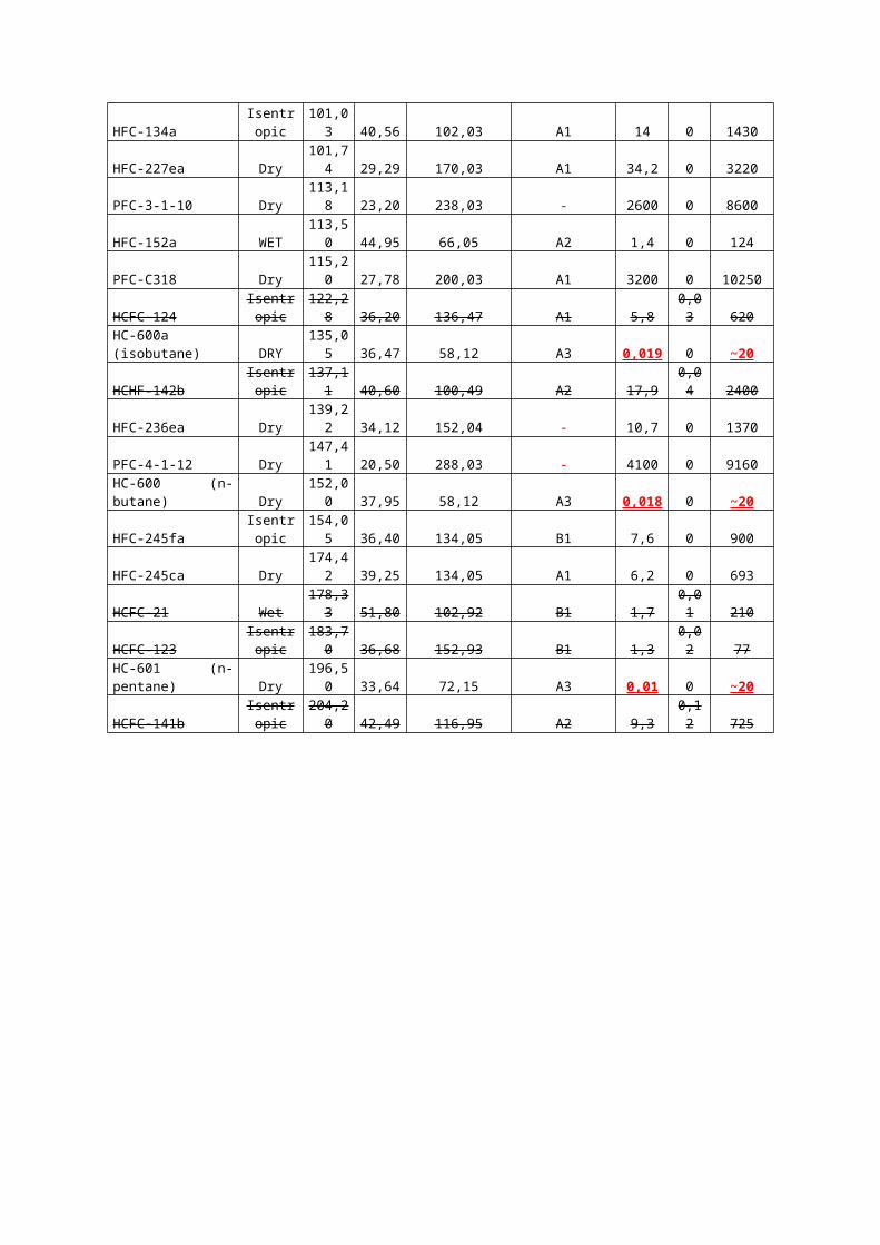
Later Cayer et al. [66] expanded his model for CO2, ethane and R125 and added 2 more performance indicators: specific net output and relative system cost. The independent parameters were the maximum cycle pressure and temperature and the net power output. The parametric studies revealed that it is not possible to simultaneously optimize all performance indicators and that the design value must be a matter of choice. A comparison of optimum indicators for the three fluids shows that none outperforms the other two on all counts. Thus, R125 had the best thermal efficiency, ethane the highest specific net power output and R125 the lowest UA, surface and cost. The CO2 had a higher total UA but a lower specific net output than ethane.

Wang J. et al. [63] performed a parametric exergy analysis for transcritical CO2 by means of a genetic algorithm to recover as much waste heat as possible. They found that key thermodynamic parameters, such as turbine inlet pressure, turbine inlet temperature and environment temperature have significant effects on the performance of the supercritical CO2 power cycle and exergy destruction.

Zhang S. et al. [65] did a parameter optimization and performance comparison of 16 working fluids in subcritical and transcritical ORCs for low-temperature geothermal power generation. Five performance indicators were used as objective functions: thermal efficiency, exergy efficiency, recovery efficiency, heat exchanger area per unit power output (APR) and levelized energy cost (LEC). The transcritical cycles had a lower thermal efficiency, but a much lower vapour expansion ratio, which indicates less turbine stages, smaller expanders and no supersonic flows. Also fluids in transcritical cycles recovered more available thermal power and could maximize the utilization of the geothermal heat source. The transcritical cycle working with R125 has excellent economic and environmental performance.

To compare cycles under equal operating conditions it is common to use the same boiling and condensing temperatures. However, for a cycle with sensible heat addition or rejection temperature, such as a transcritical power cycle, the heating (and cooling) processes take place with gliding temperature instead of isothermal. Therefore, an equal reference temperature is needed to compare subcritical and transcritical cycles equally. For a cycle with gliding temperatures, the mean heat addition temperature will be lower than the maximum heat addition temperature, while the mean heat rejection temperature will be higher than the minimum heat rejection temperature as well. Consequently, the thermodynamic mean temperatures can be used to define the reference temperature in heat addition or heat rejection process for such a cycle [81]. The thermodynamic mean temperatures for the heating and cooling processes of a cycle with gliding temperature can be defined as follows, respectively:

T eq ,max=h3−h2(a)s3−s2(a)

And

T eq, min=h4(a)−h1s4(a)−s1

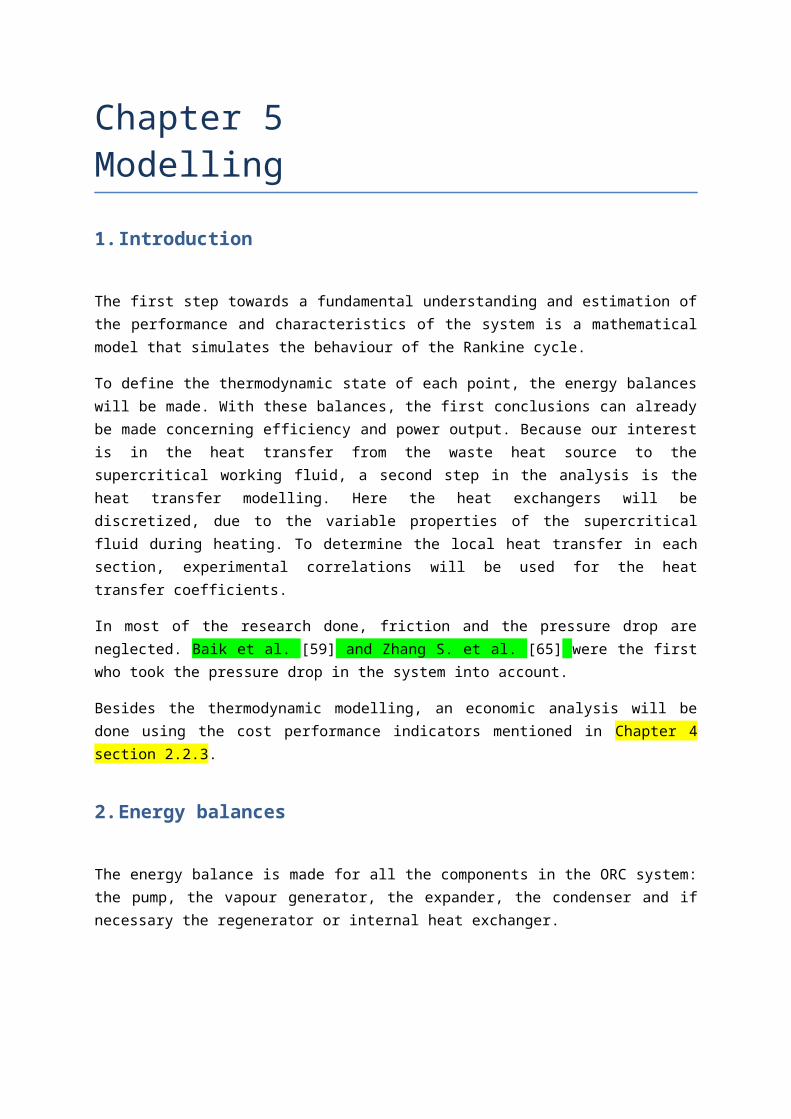
2.1 Energy analysis

In the energy analysis, the objective is to determine the thermal efficiency and the specific net power output. The first law of thermodynamics only depends on the states of the working fluid at different points in the cycle and is not influenced by the working fluid mass flow rate and the net power output.

Cayer et al. [66] found that the thermal efficiency and specific net power output increase with increasing maximum cycle temperature (turbine inlet temperature). An optimization for the maximum cycle temperature is not required, because it will lead a value equal to the inlet temperature of the heat source, and will require an infinitely large transcritical heater for this temperature.

Varying the maximum cycle pressure (turbine inlet pressure), it clear as can be seen in Figure 29 and Figure 30 a maximum occurs for the thermal efficiency and specific net power output. The corresponding optimizing maximum pressure increases with increasing maximum cycle temperature. Furthermore, the optimum specific output is at a lower maximum pressure than the optimum thermal efficiency.

Figure 29: Transcritical CO2: Thermal efficiency versus maximum pressure for different Tmax [66].

Figure 30: Transcritical CO2: Specific net power output versus maximum pressure for different Tmax [66].

For free heat sources, the focus should be in maximizing the specific output, rather than the thermal efficiency.

A comparison between transcritical CO2, R125 and ethane is given in Figure 31 and Figure 32.

Figure 31: Thermal efficiency: comparison between CO2, R125 and ethane (Tmax=95°C) [66].

Figure 32: Specific net power output: comparison between CO2, R125 and ethane (Tmax=95°C) [66].

Figure 31 shows that R125 achieves a maximum thermal efficiency above 10%, which is significantly higher than for CO2 and ethane and also corresponds with a lower maximum cycle pressure. The ethane and the carbon dioxide achieve similar maximum thermal efficiencies near 8.5% but the ethane needs a lower pressure.

The maximum outputs (Figure 32) for CO2 and R125 are significantly lower than the output for ethane as working fluid. The pressure at which the maximum outputs are obtained is lowest for R125 and highest for CO2.

Wang J. et al. [63] investigated the net power output of transcritical CO2 and R125 (Figure 33).

Figure 33: Optimized carbon dioxide transcritical cycle (left) and optimized R125 transcritical cycle (right) [63].

The net power of the R125 transcritical cycle is around 14% greater than that of the carbon dioxide cycle. The main reasons are the higher cycle pressure of CO2, because the increased turbine power of the carbon dioxide cycle cannot compensate for the pumping power increase and also the CO2 cycle has a greater exergy destruction of the pump.

Chen H. et al. [47] found that the thermal efficiency of transcritical R32 is higher than carbon dioxide for the same temperature and at a lower maximum working pressure (Figure 34). R32 has a

maximum limiting pressure for each turbine inlet temperature, because of the allowed vapour quality in the turbine (here x ≥ 95%).

Figure 34: Thermal efficiencies of a CO2- and R32-based transcritical Rankine cycles [47].

2.2 Exergy analysis

The energy analysis does not take the quality of the heat exchange in the vapour generator and condenser into account, so a second law analysis is required. To characterize the heat transfer process, the mass flow rate of the working fluid, heat source and cold source are necessary.

An exergy destruction distribution analysis showed that around 50% of the irreversibility takes place in the vapour generator, 27% in the turbine, 11% in the condenser, 7% in the pump and less than 5% in the regenerator. This distribution is essentially the same for all values of the high pressure and . In view of these results, efforts should be made to improve the temperature matching between the heat source and the working fluid in the evaporator

Cayer et al. [66] investigated the influence of the turbine inlet temperature and pressure and the net power output of the exergy efficiency (ηex=f (Tmax , pmax∧α )). For a fixed net power output , the exergy efficiency increases with increasing maximum cycle pressure and maximum cycle temperature. The optimizing maximum pressure is almost identical for the thermal and exergy efficiency.

For a fixed maximum cycle temperature (95°C), the exergy efficiency increases with increasing net power output. Moreover, the high pressure which maximizes ex is relatively independent of .

Figure 35: Exergy efficiency versus maximum pressure for > 0.21 with Tmax = 95°C [66].

For high values of an important phenomenon occurs at low and high values of the maximum pressure: the specific net output for such pressures being low, the working fluid mass flow rate and the heat extracted from the heat source increase in order to generate the high net power output corresponding to . Since the heat source capacity is limited, extracting more heat results in a reduction of its temperature throughout the vapour generator. However this temperature cannot be lower than the corresponding temperature of the carbon dioxide. This condition limits the acceptable range of values for the maximum pressure.

An exergy destruction distribution analysis showed that around 50% of the irreversibility takes place in the vapour generator, 27% in the turbine, 11% in the condenser, 7% in the pump and less than 5% in the regenerator. This distribution is essentially the same for all values of the high pressure and . In view of these results, efforts should be made to improve the temperature matching between the heat source and the working fluid in the evaporator

Wang J. et al. [63] investigated the effect of turbine inlet pressure, turbine inlet temperature and environment temperature on the exergy efficiency for different heat source temperatures.

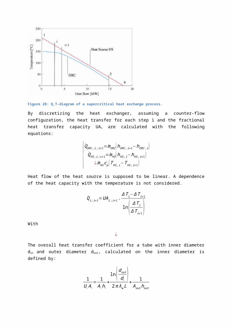
Figure 36: Exergy efficiency versus turbine inlet pressure for various heat source temperatures [63].

The effect of the turbine inlet pressure shows a maximum exergy efficiency. As the enthalpy drop across the turbine increases as the pressure ratio increases, the turbine power output increases. By subtracting pump input from the turbine power output, the net power output increases. From a certain value for the turbine inlet pressure, a decrease in vapour flow rate is generated by vapour generator, resulting in a decrease of the net power output and so also the exergy efficiency.

As can be seen on Figure 36 the exergy efficiency increases as heat source temperature increases.

Furthermore, the exergy efficiency increases as the turbine inlet temperature increases (Figure 37).

Figure 37: Exergy efficiency versus turbine inlet temperature for various heat source temperatures [63].

By studying the effect of the environment temperature on exergy efficiency, it was noticed that the exergy efficiency decreases with an increase in environment temperature. The reason for this is that

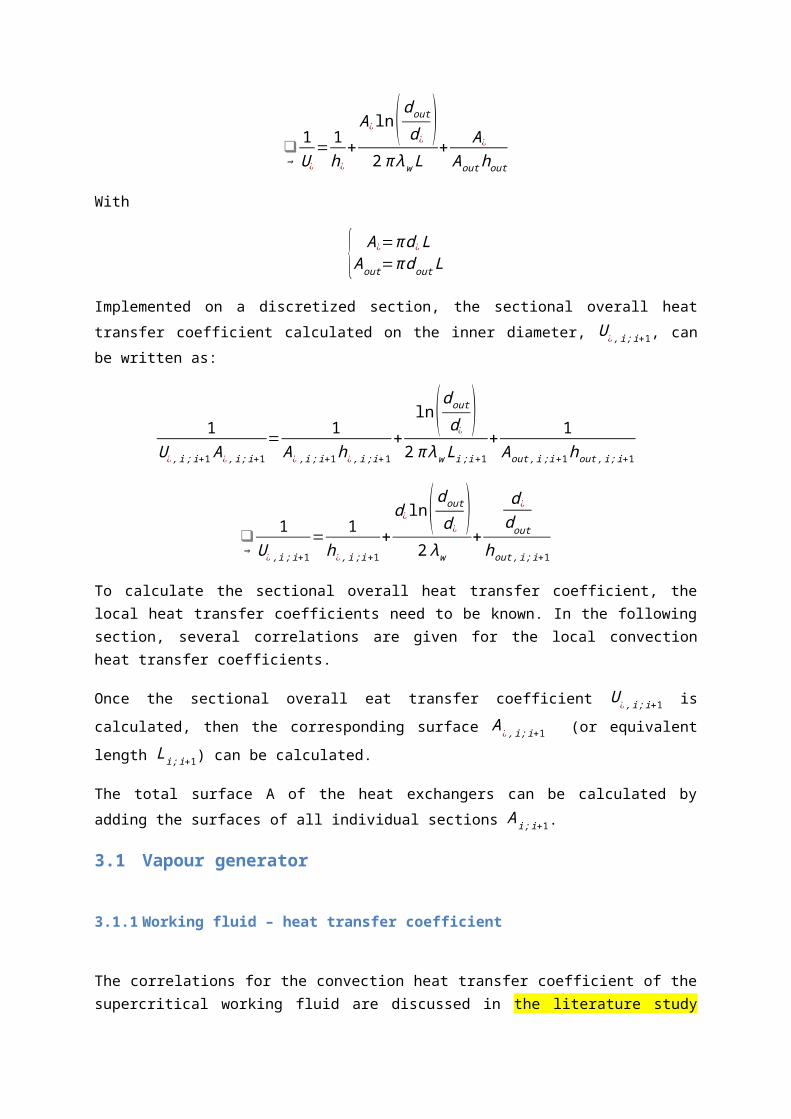
an increase in environment temperature results in an increase in condensing pressure, which reduces the turbine power

Figure 38: Exergy efficiency versus environment temperature for various heat source temperatures [63].

Wang et al. took a close look at the exergy destruction for each component in function of the thermodynamic parameter turbine inlet pressure and temperature and environment temperature and found that the biggest exergy destruction occurs in vapour generator, followed by the turbine, then the condenser and at last the pump. The turbine inlet pressure had the biggest effect on exergy destruction as can be seen in Figure 39.

Figure 39: Exergy destruction in each component versus turbine inlet pressure [63].

As turbine inlet pressure increases, the exergy destruction in the vapour generator decreases. The exergy destruction in the pump and turbine increase, because an increase in the turbine inlet pressure results in an increase in pressure difference through the turbine or pump. In the condenser a decrease in exergy destruction is noticed, because the turbine outlet temperature decreases. This could result in a decrease in heat transfer temperature difference for the condenser.

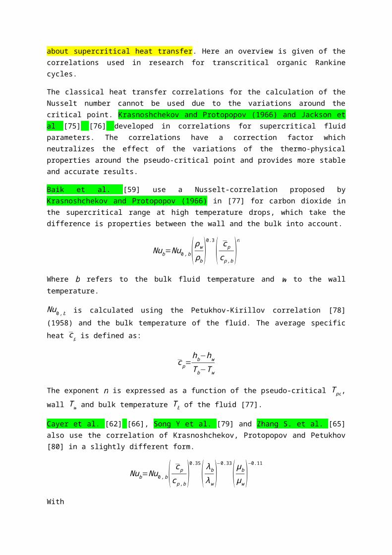
Figure 40: Exergy destruction in each component versus turbine inlet temperature [63].

As the turbine inlet temperature increases (Figure 40), the exergy destruction in the vapour generator decreases, because an increase in the turbine inlet temperature can result in a decrease in the heat transfer temperature difference for the vapour generator. Further, the exergy destruction in the pump and turbine decreases and in the condenser an increase is noticeable, because turbine outlet temperature increases, thus, the heat transfer temperature difference in the condenser increases.

The influence on the exergy destruction as the environment temperature increases (Figure 41) is visible as a decrease in exergy destruction in the pump and turbine, because the condensing pressure increases, thus, the pressure differences through the turbine and the pump decrease. In the condenser itself, the exergy destruction increases, because the turbine outlet temperature increases, and this results in an increase in the heat transfer temperature difference for the condenser.

Figure 41: Exergy destruction in each component versus environment temperature [63].

2.3 Recovery efficiency

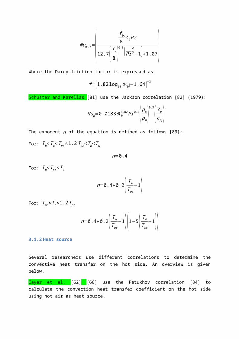
The recovery efficiency is an indicator for evaluating the ratio of available energy recovered from the heat source.

Zhang S. et al. [65] used this performance indicator for different working fluids (Figure 42). The highest recovery efficiency was delivered by R218 followed by R41 and R125. These fluids in transcritical power cycle recovered much more available thermal power and could maximize the utilization of the geothermal source. So the favoured working fluids in terms of geothermal utilization were the fluids in transcritical power cycle with R218, R41 and R125.

Figure 42: Recovery efficiency of different working fluids under their optimized operation parameters [65].

2.4 Total heat transfer capacity UA

As mentioned before the heat exchangers are discretized so that the variations of the properties can be considered constant in each step. The discretization is performed by dividing the overall enthalpy change for one of the streams in N equal differences h.

Determination value of n calculation error (reference = 1000 points)

Near pcrit for R134a: partitioning into 32 sections (3.24% error 52.6% 1 section) Near pcrit for R227ea: partitioning into 32 sections (2.35% error 50.67% 1 section) As pmax ↑ calculation error ↓ (32 8 sections for ± same error), due to a smoother variation

of the thermophysical properties under greater pressure around pseudo-Tcrit. Here 500 sections are used error 0.01%

By analysing the heat transfer capacity as performance indicator, Cayer et al. [62] showed that the use of an internal heat exchanger is in most of the cases not practical, because the new UA added by the internal heat exchanger does not fully compensate the obtained reduction at the vapour generator.

For a fixed net power output, Cayer et al. [66] saw that the total UA varies significantly with the maximum cycle pressure and temperature. The optimizing maximum cycle temperature is not equal

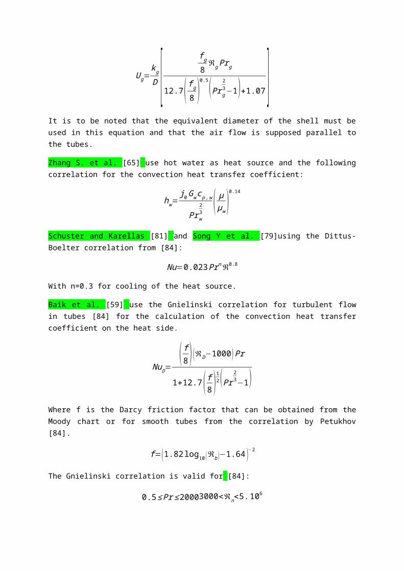
to the inlet temperature of the heat source (as in the thermal and exergy analysis), because this would yield an infinitely large vapour generator. Low values of the maximum cycle temperature also doesn’t provide low values for the total UA, because in order to obtain the net power output, a higher mass flow rate is required (due to the lower values of the specific output at low Tmax). If the mass flow rate increases, the temperature difference between the fluids decrease and the total heat transfer capacity increased accordingly.

There exists an optimum maximum cycle temperature as well as an optimum maximum cycle pressure that minimizes the total UA.

Cayer et al. [66] compared three working fluids (CO2, R125 and ethane) and found that the lowest values of the total heat transfer capacity is obtained with R125, followed by ethane which shows a slightly lower UA than carbon dioxide except for very high net power outputs.

Schuster and Karellas [23] found that maximum cycle temperatures with good system efficiencies and low exergy losses need the highest heat transfer capacities.

2.5 Heat exchanger surface

To determine the surface A of the heat exchangers, the heat transfer coefficients for the fluids need to be calculated using the correlations presented in Chapter 5 and the literature study about supercritical heat transfer.

Each heat exchanger is considered as a counter-flow shell and tubes with one pass for all the streams. The vapour generator transfers the heat from the waste heat source to the working fluid. The high pressure working fluid flows inside the tubes and the air flows in the shell. Because of the poor heat transfer coefficient of air, longitudinal fins can be added on the outside of each tube. The number of tubes and the shell diameter are obtained from the mass balance equations by fixing the minimum velocity for example at 0.5 m/s for the liquid working fluid and the maximum velocity for example at 30 m/s for the hot entering air.

The condenser modelling is similar to the vapour generator with a few exceptions. The working fluid still flows inside the tubes because of its higher pressure and the water in the shell. However, this time the longitudinal fins are positioned inside the tubes because of the good transfer properties of water and the risk of fouling if fins are installed on the water side. The number of tubes and the shell diameter are obtained by assuming a minimum velocity of for example 1.5 m/s for the saturated liquid working fluid and a maximum velocity of for example 3 m/s for the cooling water. The condenser is still divided into two sections as in the finite size analysis.

Modelling of the regenerator (if applicable) follows the same methodology as the two preceding heat exchangers. The higher pressure working fluid from the pump circulates inside the tubes and the lower pressure one from the turbine in the shell. The fins are located inside the tubes to reduce the regenerator size and facilitate assembly. The minimum velocity of the cold stream working fluid is set for example to 1.5 m/s and the maximum velocity of the supersaturated working fluid for example at 10 m/s.

Cayer et al. [62] use the Petukhov’s correlation [84] for the low pressure working fluid and Krasnoshchekov–Protopopov’s correlation (see literature study for supercritical heat transfer) for the supercritical working fluid coming from the pump.

The effect of the maximum cycle pressure on the total heat transfer area A is quasi the same as on the total heat transfer capacity UA, but the maximum cycle temperature to minimize the total area is not the same as for minimising the total heat transfer capacity (Cayer et al. [66]).

Figure 43: Total area versus maximum pressure for different Tmax with =0.2 [66].

As can be seen on Figure 44, the minimum total surface behaves linear for low values of the net power output and exponential for higher . The linearity is due to the presence of the condenser. A significant difference is noticed in the relative importance of the two heat exchangers. The vapour generator surface is higher for a large range of and definitely dominant for above 0.2 while its UA exceeds that of the condenser only when approaches its upper limit. This can be explained by the significantly greater heat transfer coefficients in the condenser which reduce the relative importance of its area despite its higher UA value.

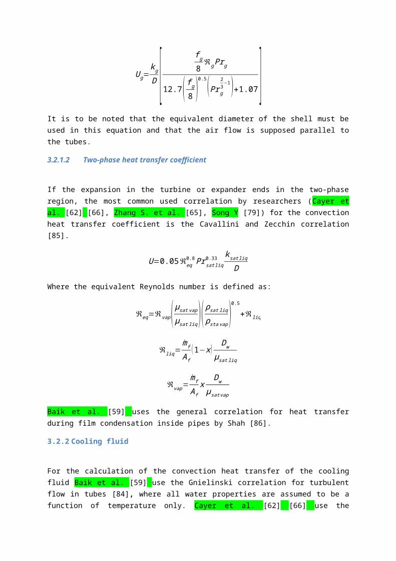
Figure 44: Optimized total area and corresponding values for the heat exchanger [66].

However, in opposition to the results for the total heat transfer capacity UA, carbon dioxide as working fluid requires a smaller heat exchanger surface than ethane, which indicates that the carbon dioxide has better heat transfer properties. The smallest heat transfer area was found for R125.

Figure 45: Comparison of minimum total heat exchange surface [66].

2.6 Thermo-economic analysis

The economics of an ORC system is linked to the thermodynamic properties of the working fluid. A bad choice of working fluid can lead to a less efficient and expensive power unit.

As mentioned already in Chapter 4, Zhang S. et al. [65] and Cayer et al. [66] were one of the first who performed a thermo-economic parameter analysis for a selection of working fluids in transcritical organic Rankine cycles (R134a, R143a, R218, R125, R41, R170, ethane and CO2).

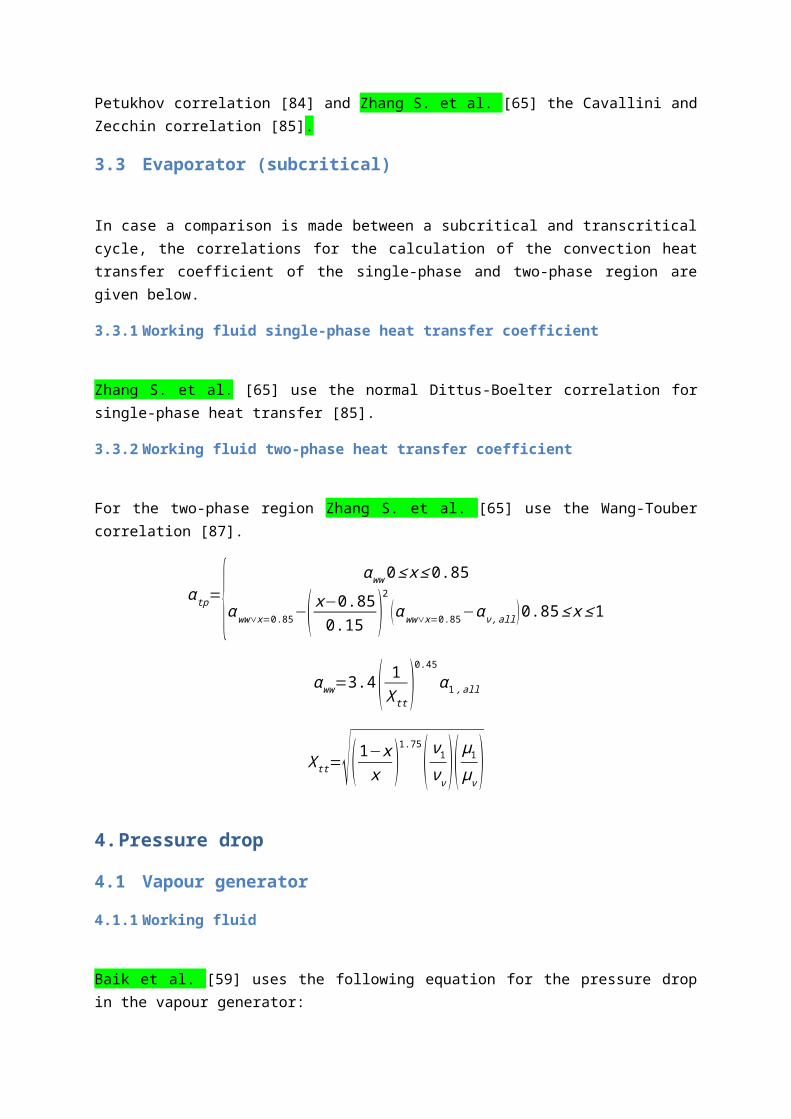
Cayer et al. [66] use well-estimated purchase prices for the major components of the cycle (pump, turbine and heat exchangers) as the representative of the complete life cycle cost, even if it is just a fraction of the actual total cost.

Zhang S et al. [65] consider the total cost of the heat exchangers representative of the complete system cost of an ORC, because 80-90% of the system capital cost can be assigned on the heat exchangers [68] [69] [70].

Two economic performance indicators can be used for evaluation of a power system:

APR LEC

The relative total cost in over a range of maximum cycle pressures and maximum cycle temperatures (for a fixed net power output) can be seen in Figure 46.

Figure 46: The relative total cost in over a range of maximum cycle pressures and maximum cycle temperatures with = 0.2 [66].

The optimising maximum pressure is significantly lower than the corresponding values determined in all the previous analyses (energy, exergy, total heart transfer capacity and heat exchange surface). The reason for this result is the important dependence of the turbine and pump costs on the pressure, because their prices rapidly increase when the pressure is augmented. On the other hand, at low pressures the heat exchangers’ surface increases and consequently so does their cost.

By varying the net power output (Figure 47) under optimized conditions, it can be observed that the total relative cost increases linearly with the net power output for low values of and exponentially for higher values of . This behaviour is similar to that observed in the analysis of the heat exchange area. Furthermore, the total cost tends towards infinity as approaches its maximum value. This rapid augmentation of the cost is mainly due to the vapour generator. Nevertheless, for most of the acceptable values of , the relative cost of the turbine is definitely dominant, because the price of this component is highly dependent on the maximum pressure.

Figure 47: Optimised relative cost and corresponding values for each component [66].

Furthermore, Cayer et al. [66] compared the relative cost per net power output for CO2, R125 and ethane (Figure 48) and it shows that the relative cost per kW with R125 is about 20% lower than the other two fluids.

Figure 48: Comparison of minimum relative cost per kW [66].

Zhang S et al. [65] also compared a series of working fluids (Figure 49) and it was found that in a transcritical power cycle system, the LEC was the lowest for R143a, R125 and R41 and was similar with that of R152a in a subcritical ORC. The carbon dioxide had a much higher operating pressure, which resulted in additional expenses in the plant design, leading to a high objective function value.

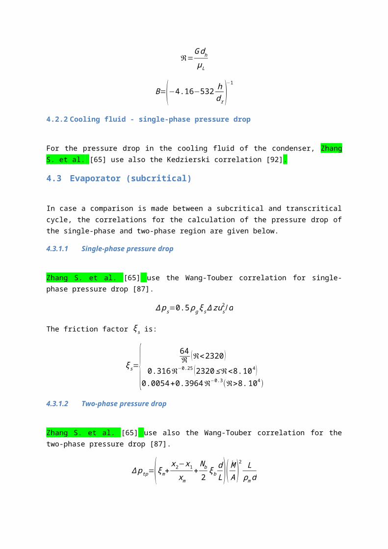
Figure 49: The LEC value of different working fluids under their optimised operation conditions [65].

Among the fluids in transcritical power cycle, R143a was not acceptable because the heating pressure range was limited by the turbine outlet quality. R41 showed favourable performance except for its flammability. These comparisons indicated that R125 in the transcritical power cycle system was preferable since it offered lower LEC, reduced more CO2-emission and cuts down more petroleum consumption.

Zhang S et al. [65] also use the APR as objective function, which is the ratio of total heat exchanger area to net power output (Figure 50).

Figure 50: The APR value of different working fluids under their optimised operation conditions [65].

In transcritical power cycle, R143a exhibited the least APR value and was a cost-effective fluid. R170 provided the highest APR value, about 59% larger than that of R143a. Among the fluids considered, R41 produced the highest net power output, but the heat exchanger area was 82.5% larger than that of R143a. As a result, R41 gave the APR value of 31.7% higher than that of R143a. To demonstrate the differences in the subcritical ORC and the transcritical power cycle, the economic performance comparison was conducted and it was observed that the choice of working fluid could greatly affect

the power plant cost. Fluids in a transcritical power cycle system took the advantage of high net power output. For example, the net output power of R143a was 28.7% and 23.8% larger than that of R152a and R123, respectively. However, due to the large heat absorption capacity, more heat exchanger area was required in transcritical power cycle. The heat exchanger area required for R143a was 57.4% and 9.8% larger than that of R152a and R123, respectively. As a result, the objective function value of R143a was 23% larger than that of R152a, but 14.8% smaller than R123.

2. Fluid selection

In Table 5 (chapter 4) an overview of working fluids was given suitable for a transcritical power cycle. Table 6 shows a reduced overview of the working fluids that can be used in transcritical cycles, according to the temperature range of the waste heat stream. Working fluids which will be phased out, working fluids with a low molecular weight, a very low critical temperature and a high flammability have been deleted.

Table 6: Overview of potential working fluids for transcritical ORCs

Physical data Safety data Environmental data

Name Type Tcrit (°C)pcrit

(bar)Molecular

weight (g/mol)ASHRAE 34

safety groupATL (yr) ODP

GWP (100 yr)

HFC-23 Wet 26,14 48,30 70,01 A1 270 0 14800

R-747 (CO2) Wet 31,10 73,80 44,01 A1 >50 0 1

HFC-125 Wet 66,02 36,20 120,02 A1 29 0 3500

HFC-410A - 70,20 47,90 72,58 A1 16,95 0 2088

PFC-218 Isentropic 71,89 26,80 188,02 A1 2600 0 8830

HFC-143a Wet 72,73 37,64 84,04 A2 52 0 4470

HFC-32 Wet 78,11 57,83 52,02 A2 4,9 0 550

HFC-407C - 86,79 45,97 86,20 A1 15657 0 1800

HFC-134aIsentropi

c 101,03 40,56 102,03 A1 14 0 1430

HFC-227ea Dry 101,74 29,29 170,03 A1 34,2 0 3220

PFC-3-1-10 Dry 113,18 23,20 238,03 - 2600 0 8600

HFC-152a WET 113,50 44,95 66,05 A2 1,4 0 124

PFC-C318 Dry 115,20 27,78 200,03 A1 3200 0 10250

HFC-236ea Dry 139,22 34,12 152,04 - 10,7 0 1370

PFC-4-1-12 Dry 147,41 20,50 288,03 - 4100 0 9160

HFC-245faIsentropi

c 154,05 36,40 134,05 B1 7,6 0 900

HFC-245ca Dry 174,42 39,25 134,05 A1 6,2 0 693

Chapter 7Heat exchanger designSchuster and Karellas (2012) [67] were the first to investigate the influence of ORC parameters on the heat exchanger design. The basic parameters of the design were defined in the cases of supercritical fluid parameters and the convective coefficients. The used working fluids were R134a, R227ea and R245fa. The general conclusion was that the heat transfer coefficient decreases with increasing supercritical pressure and temperature, consequently the heat exchanger area increases.

Chapter 8 Experimental organic Rankine cycleZhang X.R. et al. [42] [64] designed, constructed and tested a prototype of a CO2-based Rankine cycle powered by solar energy (Figure 51).

Figure 51: Prototype of the CO2-based solar-powered Rankine cycle (above) and a sketch of the evacuated solar collector (below) [42] [64].

A schematic diagram of the experimental prototype is shown in Figure 52.

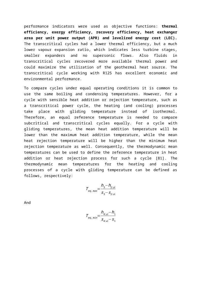
Figure 52: Schematic diagram of the prototype machine system [42] [64].

The prototype is mainly comprised of evacuated solar collector arrays, a throttling valve, heat exchangers 1 and 2 (CO2/water heat exchanger), liquid CO2 feed pump, cooling tower and measurement and data acquisition system.

Supercritical CO2 actually has physical properties somewhere between those of a liquid and a gas. So it is difficult to decide whether a turbine of a gas or a liquid type should be used for the Rankine cycle using supercritical CO2. Therefore, in the prototype, a throttling valve was used, instead of a turbine, in order to study the cycle performance. The throttling valve can provide various extents of opening for the cycle loop in order to simulate pressure drop occurring in realistic turbine condition and consequently a thermodynamic cycle can be achieved.

To effectively heat CO2 to a higher-temperature supercritical state in the prototype, all-glass evacuated solar collectors with a U-tube heat removal system are used, shown in Figure 51. These collectors consist of a glass envelope (38 mm in diameter) over an inner glass tube (27 mm in diameter) coated with a selective solar absorber coating. This coating with a high solar absorbance 0.927 and a low emissivity 0.193 is applied on the vacuum side of the inner glass tube. The absorbed heat is conducted through the inner glass tube wall and then removed by heat removal fluid in a metal U-tube (3.6 m in length and 0.005 m in internal diameter) inserted in the inner tube with an aluminium fin (1.7 m in length) connecting the outlet arm of the U-tube to the inner glass tube. In this prototype, evacuated solar collector of 29.0 m2 is used (efficient area of 9.6 m2). The collector used is commercial product provided by Showa Denko K. K., designed to have a maximum allowable work pressure of 12 MPa and have a maximum working temperature of 250°C.

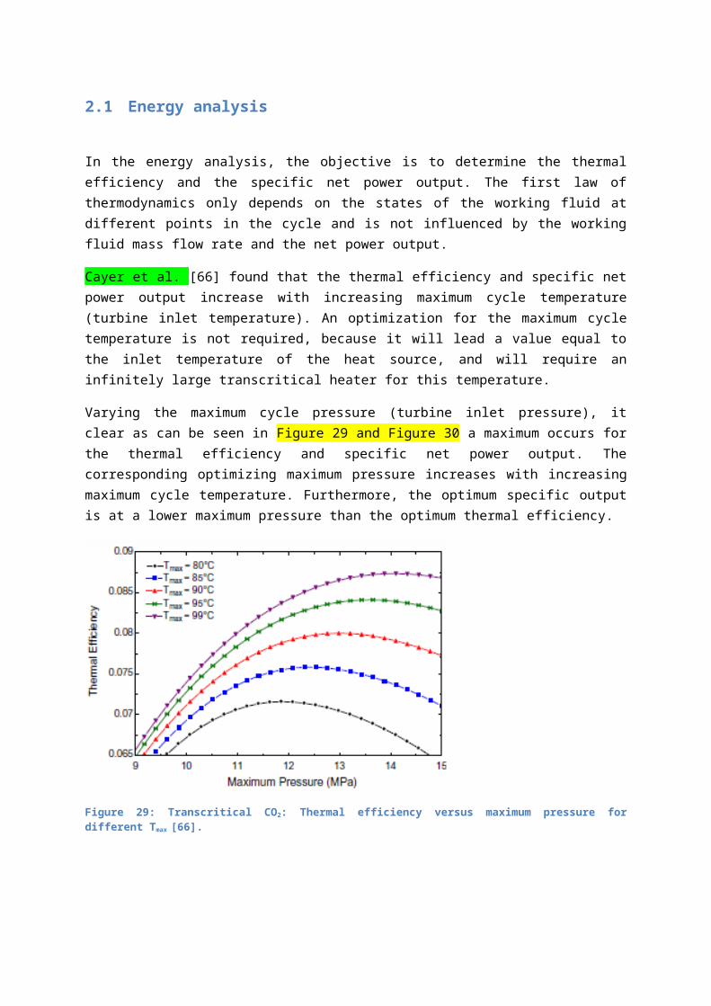
A piston pump is used for feeding liquid CO2 in the prototype. This canned motor feed pump can provide a maximum operating pressure of 12 MPa and flow rate of 0.03 kg/s, respectively. A Coriolis-effect mass flow meter is used in the cycle to monitor and record the mass flow of liquid CO 2, which also has a maximum permissible operating pressure of 12 MPa. The flow meter is installed in the downstream side of the CO2 feed pump, as shown in Figure 52. It provides a measurement range of 0.09–1.0 kg/min with an accuracy of ±0.1%.

Five T-type thermocouples and five pressure transmitters were mounted at different positions in the CO2 flow to measure its temperatures and pressures, with an accuracy of ±0.1°C for temperature measurements and ±0.2% for pressure measurements. Measured quantities include the following: CO2 temperatures and pressures at the collector outlet; at the outlet of the throttling valve; at the outlet of the heat exchanger 1; at the outlet of the heat exchanger 2; at the outlet of the CO 2 feed pump. The measuring points of these sensors are also shown in Figure 52.

A mechanical-draft water cooling tower (with a cooling capacity of 22 kW) is used as a heat sink, dissipating heat recovered from the Rankine cycle to the ambient. In order to achieve a good heat exchange between CO2 and water, shell and tube design is used for the heat exchangers 1 and 2, with tube side of CO2 and shell side of water. The temperature of water used to recover heat in the high-temperature heat recovery system is determined by CO2 temperature and cooling capacity of the cooling tower. Hence during the experiment the water flow rate and cooling capacity are adjusted to provide a suitable water temperature for the heat recovery.

There are four platinum resistor temperature sensors mounted to measure inlet and outlet water temperatures of the heat exchangers, with an accuracy of ±0.15 + 0.0002|t|°C. Water flow rates of the heat exchangers 1 and 2 are measured by two water flow meters mounted at the outlets of the heat exchangers, with an accuracy of ±0.5%.

During a typical experiment, water pumps are first turned on and the water flow rates are adjusted. Then the CO2 feed pump is switched on and the opening of the valve is adjusted to the expected extent. The CO2 pump is turned off after the test is finished. This is done only after adjusting the valve to a state of full open. Finally the water pumps are turned off.

During the experiment, the two major error sources are:

Temperature, pressure and flow rate measurement accuracy; Error resulting from data logging and reading by the computer.

The error of data logging and reading include as follows: ±0.1% for CO2 temperature; ±0.3% for CO2

pressure; ±0.3% for CO2 mass flow rate; ±0.2% for water temperature; ±0.3% for water flow rate; ±0.3% for solar radiation; ±0.2% for atmospheric temperature.

A detailed error analysis indicates that the maximum uncertainty in the performance parameters is less than ±3.0%. Therefore, these errors are acceptable for the present study.

Thermal insulation coating applied on all the carbon dioxide and water loops to reduce heat losses from the piping.

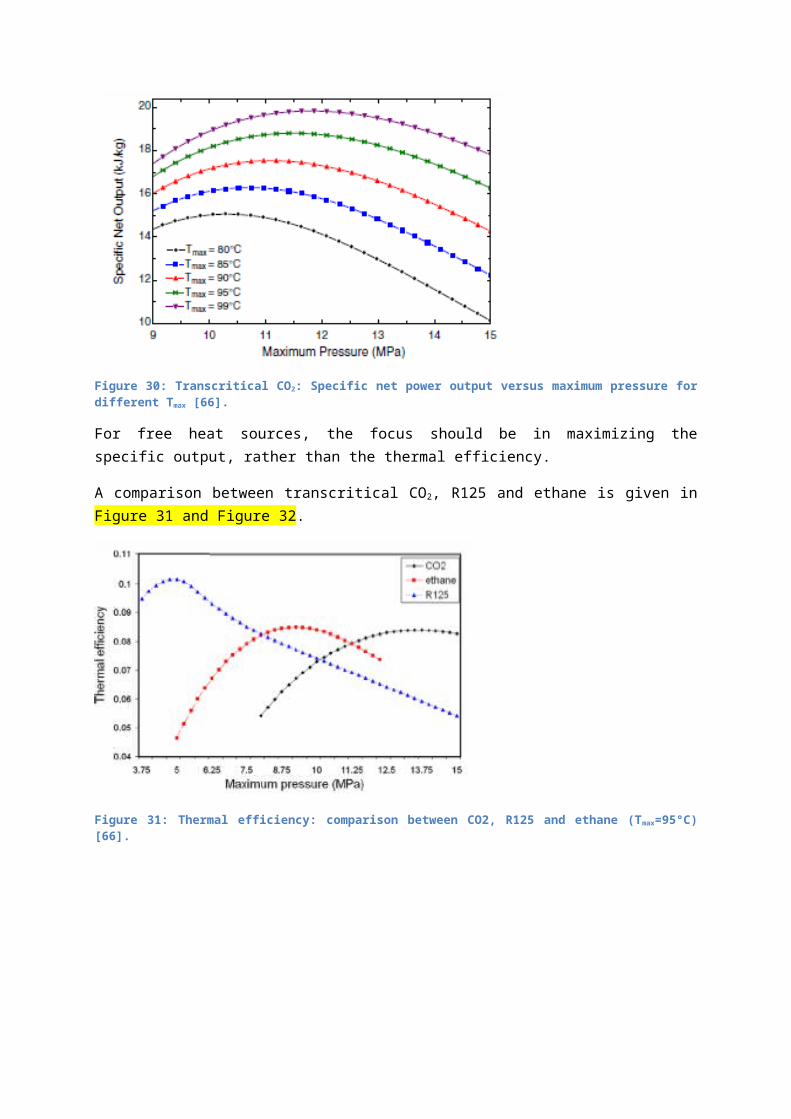
References

[1] Stricker Associates Inc. Market study on waste heat and requirements for cooling and refrigeration in Canadian industry.2006.

[2] TeTra-Symposium 2009.

[3] Mckinsey 2009.

[4] Masokin 2007.

[5] „ORCycle,” [Online]. Available: www.orcycle.be. [Geopend 05 11 2012].

[6] Wali E. Optimum working fluids for solar powered Rankine cycle cooling of buildings. Solar Energy 1980;25:235–41.

[7] Hung TC, Shai TY, Wang SK. A review of organic rankine cycles (ORCs) for the recovery of low-grade waste heat. Energy 1997; 22(7):661e7.

[8] B.F. Tchanche et al. Low-grade heat conversion into power using organic Rankine cycles – A review of various applications Renewable and Sustainable Energy Reviews 15 (2011) 3963–3979.

[9] Andersen WC, Bruno TJ. Rapid screening of fluids for chemical stability in organic Rankine cycle applications. Industrial and Engineering Chemistry Research 2005;44:5560–6.

[10] Schuster A, Karellas S, Supercritical Fluid Parameters in Organic Rankine Cycle Applications, International Journal of Thermodynamics 2008; 11(3): 101-108.

[11] Mathias JA et al., Experimental testing of gerotor and scroll expanders used in, and energetic and exergetic modeling of, an organic Rankine cycle. Journal of Energy Resources Technology 2009;131(3):012201–12209.

[12] Duvia, A., Gaia M. (2002): ORC plants for power production from 0,4 MWe to 1,5 MWe: technology, efficiency, practical experiences and economy. 7th Holzenergie Symposium, Zürich, Switzerland, 18. October 2002.

[13] Karl, J. (2004): Decentralised energy systems, new technologies in liberalised energy market Dezentrale Energiesysteme , (Neue Technologien im liberalisierten Energiemarkt) Oldenbourg Wissensschaftsverlag, München,. (in German).

[14] Turboden High Efficiency Rankine for Renewable Energy and Heat Recovery available at: http://www.turboden.it/orc.asp (Date of access 22.10.2012).

[15] Drescher I., Brüggemann D. (2007): Fluid selection for the Organic Rankine Cycle (ORC) in biomass power and heat plants, Applied Thermal Engineering 27 (2007) 223-228..

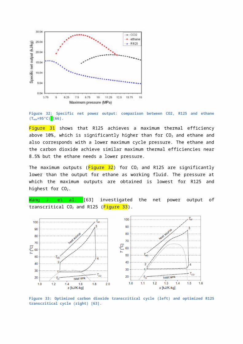
[16] Barbier E. Nature and technology of geothermal energy: a review. Renewable Sustainable Energy Rev 1997;1(1–2):1–69.

[17] Barbier E. Geothermal energy technology and current status: an overview. Renewable Sustainable Energy Rev 2002;6:3–65.

[18] Broßmann E, Eckert F, Möllmann G, Technical concept of the geothermal power plant Neustadt-Glewe. (technisches Konzept des geothermischen Kraftwerks Neustadt-Gelewe).Berlin, Germany; http://www.geothermie.de/gte/gte43/technisches_konzept_des_geotherm.htm.

[19] Lund, J (2005). W.: Combined Heat and Power plant Neustadt-Glewe, Germany. GHC, Bulletin June.

[20] Sylvain Quoilin, Sustainable Energy Conversion Through the Use of Organic Rankine Cycles for Waste Heat Recovery and Solar Applications, Liège, October 2011.

[21] Fachagentur nachwachsende Rohstoffe e.V. (2004) (ed.): Assistance for Biogas production and use (Handreichung Biogasgewinnung und – nutzung). Leipzig,. (in German).

[22] R. Vescovo, „Cogeneration and on-site power production,” Turboden, 01 03 2009. [Online]. Available: http://www.cospp.com/articles/print/volume-10/issue-2/features/orc-recovering-industrial-heat-power-generation-from-waste-energy-streams.html. [Geopend 22 10 2012].

[23] Schuster A, Karellas S, Efficiency optimization potential in supercritical Organic Rankine Cycles, Energy 2010 (35): 1033-1039.

[24] DiPippo R. Ideal thermal efficiency for geothermal binary plants. Geothermics 2007;36(3):276–85.

[25] Larjola J. Electricity from industrial waste heat using high-speed organic Rankine cycle (ORC). Int J Prod Econ.

[26] Chen Y. Novel cycles using carbon dioxide as working fluid. Licentiate thesis. Stockholm, Sweden: School of Industrial Engineering and Management; 2006.

[27] Kalina AI. Combined-cycle system with novel bottoming cycle. J Eng Gas Turb Power 1984;106:737–42.

[28] Saleh B. Working fluids for low-temperature organic Rankine cycles; Energy 32 (2007): 1210–1221.

[29] Feher EG. The supercritical thermodynamic power cycle. Energy Convers 1968;8:85–90.

[30] Gu Z, Optimization of cyclic parameters of a supercritical cycle for geothermal power generation, Energy Conversion and Management 42 (2001) 1409-1416.

[31] Gu Z, Sato H. Performance of supercritical cycles for geothermal binary design. Energy Conversion and Management 43 (2002) 961–971.

[32] Zhang XR, Yamaguchi H, Analysis of a novel solar energy-powered Rankine cycle for combined power and heat generation using supercritical carbon dioxide, Renewable Energy 31 (2006) 1839–1854.

[33] Zhang XR. Theoretical analysis of a thermodynamic cycle for power and heat production using supercritical carbon dioxide, Applied Thermal Engineering 26 (2006) 2142–2147.

[34] Chen Y, Lundqvist P, Platell P. Theoretical research of carbon dioxide power cycle application in automobile industry to reduce vehicle’s fuel consumption. Appl Therm Eng 2005;25(14–15):2041–53.

[35] UNEP, „Montreal protocol on substances that deplete the ozone layer,” 1987, reviewed in 2000.

[36] Rogers G, Mayhew Y. Engineering thermodynamics, work and heat transfer, 4th ed. Harlow: Longman Scientific &Technical; 1992 (p. 239–243).

[37] P.J. Mago, L.M. Chamra, K. Srinivasan, C. Somayaji, An examination of regenerative organic Rankine cycles using dry fluids. Applied Thermal Engineering 28 (8-9) (2008) 998e1007.

[38] ANSI/ASHRAE Standard 34, Number Designation and Safety Classification of Regfrigerants, 2008.

[39] "Global Warming Potentials". Contribution of Working Group I to the Fourth Assessment Report of the Intergovernmental Panel on Climate Change, 2007. 2007. Retrieved 2012-10-26.

[40] „Wikipedia - Ozone depletion potential,” 30 08 2012. [Online]. Available: http://en.wikipedia.org/wiki/Ozone_depletion_potential. [Geopend 26 10 2012].

[41] „Wikipedia - Atmospheric lifetime,” 23 10 2012. [Online]. Available: http://en.wikipedia.org/wiki/Greenhouse_gas#Atmospheric_lifetime. [Geopend 26 10 2012].

[42] Zhang XR, Yamaguchi H. Solar energy powered Rankine cycle using supercritical CO2. Applied Thermal Engineering 26 (2006): 2345–2354.

[43] Quoilin S. Experimental study and modeling of a low temperature Rankine cycle for small scale cogeneration. Thesis, University of Liege; 2007.

[44] Calderazzi L, di Paliano PC. Thermal stability of R-134a, R-141b, R-13I1, R-7146, R-125 associated with stainless steel as a containing material. International Journal of Refrigeration 1997;20:381–9.

[45] Liu BT. Effect of working fluids in organic Rankine cycle for waste heat recovery, Energy 29 (2004): 1207–1217.

[46] Poling BE, Prausnitz JM, O’Connell JP. The properties of gases and liquids, 5th ed. New York: McGraw-Hill; 2001.

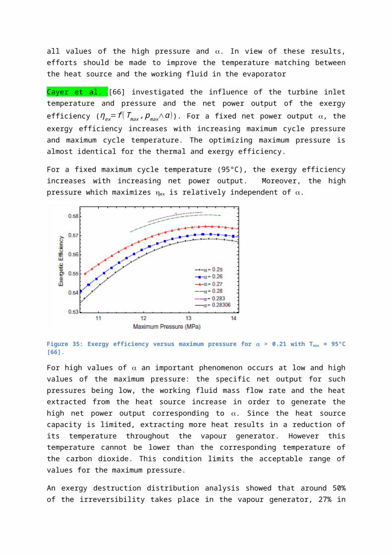
[47] Chen H, Goswami DY, Rahman M, Stefanakos EK. Energetic and exergetic analysis of CO2- and R32-based transcritical Rankine cycles for low-grade heat conversion, Applied Energy 2011; 88: 2802-2808.

[48] Chen H. et al. A review of thermodynamic cycles and working fluids for the conversion of low-grade heat. Renewable and Sustainable Energy Reviews 14 (2010) 3059–3067.

[49] Bakhtar F, Mahpeykar MR. On the performance of a cascade of turbine rotor tip section blading in nucleating steam. Part 3: theoretical treatment. Proceedings of the Institution of Mechanical Engineers Part C Mechanical Engineering Science 1997;211:195–210.

[50] Bakhtar F. On the performance of a cascade of turbine rotor tip section blading in wet steam. Part 1: generation of wer steam of prescribed droplet sizes. Proceedings of the Institution of Mech Engineers Part C Mech Engineering Science 2005;209:115–24.

[51] Bakhtar F. On the performance of a cascade of turbine rotor tip section blading in wet steam. Part 2: surface pressure distributions. Proceedings of the Institution of Mech Engineers Part C Journal of Mech Engineering Science 1997;211:531–40.

[52] Bakhtar F. On the performance of a cascade of turbine rotor tip section blading in wet steam. Part 4: droplet measurements. Proceedings of the Institution of Mech Engineers Part C Journal of Mech Engineering Science 1997;211:639–48.

[53] Goswami DY, Hingorani S, Mines G. A laser-based technique for particle sizing to study two-phase expansion in turbines. Journal of Solar Energy Engineering 1991;113:211–8.

[54] Demuth OJ. Analyses of mixed hydrocarbon binary thermodynamic cycles for moderate temperature geothermal resources, Idaho; 1981.

[55] Demuth OJ, Preliminary assessment of condensation behavior for hydrocarbon– vapor expansions which cross the saturation line near the critical point, Idaho; 1983.

[56] Chen H, Goswami DY, Rahman M, Stefanakos EK. A supercritical Rankine cycle using zeotropic mixture working fluids for the conversion of low-grade heat into power, Energy 2011; 36: 549-555.

[57] Moran MJ (2011), Fundamentals of engineering thermodynamics (7th edition). John Wiley & Sons.

[58] Chen Y, Lundqvist P, Johansson A, Platell P, A comparative study of the carbon dioxide transcritical power cycle compared with an organic Rankine cycle with R123 as working fluid in waste heat recovery, Applied Thermal Engineering 2006 (26): 2142-2147.

[59] Baik YJ, Kim M, Chang KC, Kim SJ; Power-based performance comparison between carbon dioxide and R125 transcritical cycles for a low-grade heat source; Applied Energy 88 (2011) 892–898.

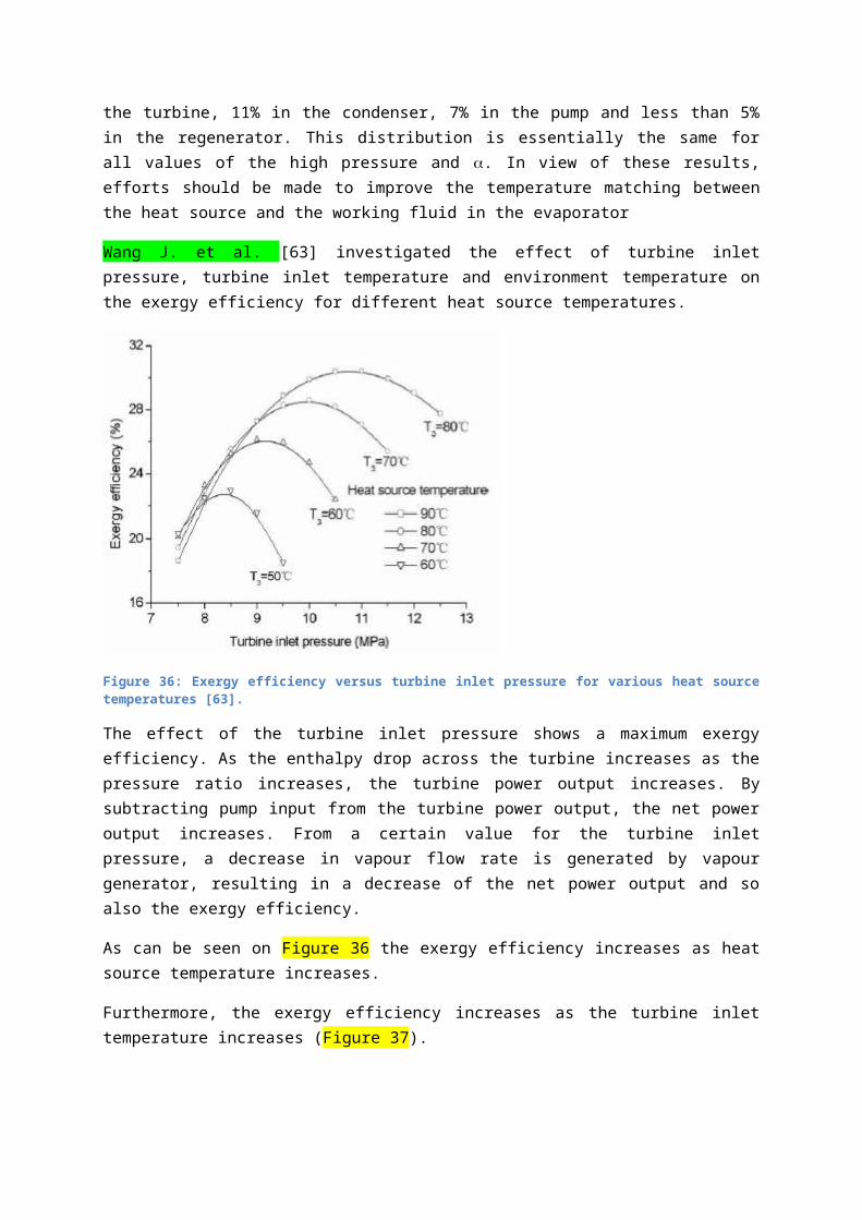
[60] Mikielewicz D, Mikielewicz J. A thermodynamic criterion for selection of working fluid for subcritical and supercritical domestic micro CHP, Applied Thermal Engineering 30 (2010) 2357e2362.

[61] Ho et al, Comparison of the Organic Flash Cycle (OFC) to other advanced vapor cycles for intermediate and high temperature waste heat reclamation and solar thermal energy, Energy 42 (2012) 213e223.

[62] Cayer, Galanis. Analysis of a CO2 transcritical power cycle using a low temperature source; Applied Energy 86 (2009): 1055–1063.

[63] Wang J, Sun Z, Dai Y, Ma S. Parametric optimization design for supercritical CO2 power cycle using genetic algorithm and artificial neural network, Applied Energy 87 (2010) 1317–1324.

[64] Zhang XR, Yamaguchi H, Experimental study on the performance of solar Rankine system using supercritical CO2, Renewable Energy 32 (2007) 2617–2628.

[65] Zhang S, Wang H, Guo T. Performance comparison and parametric optimization of subcritical Organic Rankine Cycle (ORC) and transcritical power cycle system for low-temperature geothermal power generation, Applied Energy 2011; 88: 2740-2754.

[66] Cayer E, Galanis N, Nesreddine H. Parametric study and optimization of a transcritical power cycle using a low temperature source, Applied Energy 2010; 87: 1349-1357.

[67] Schuster A, Karellas S, Leontaritis AD. Influence of supercritical ORC parameters on plate heat exchanger design, Applied Thermal Engineering 2012; 33-34: 70-76.

[68] Papadopoulos AI, Stijepovic M, Linke P. On the systematic design and selection of optimal working fluids for Organic Rankine Cycles. Appl Therm Eng 2010;30:760–9.

[69] Uehara H, Ikegami Y. Optimization of a closed-cycle OTEC plant system. J Solar Eng 1990;112:247–56.

[70] Bliem C, Zangrando F, Hassani V. Value analysis of advanced heat rejection systems for geothermal power plants. Energy Conver Eng Conf 1996.

[71] Turton R, Bailie RC, Whiting WB, Shaeiwitz JA. Analysis, synthesis and design of chemical processes. New Jersey: Prentice Hall PTR; 1998.

[72] Calm JM, Hourahan GC. Refrigerant data summary. Eng Syst 2001;18(11):74–88.

[73] Nafey AS, Sharaf MA. Combined solar Organic Rankine Cycle with reverse osmosis desalination process: energy, exergy, and cost evaluations. Renew Energy 2010.

[74] Hammer H, Röhmfeld M. Abwärmenutzung zur Krafterzeugung mittels neuer Kreislaufmedien. VDI-Bericht 415, 81–87, VDI-Verlag Düsseldorf; 1981 (in German).

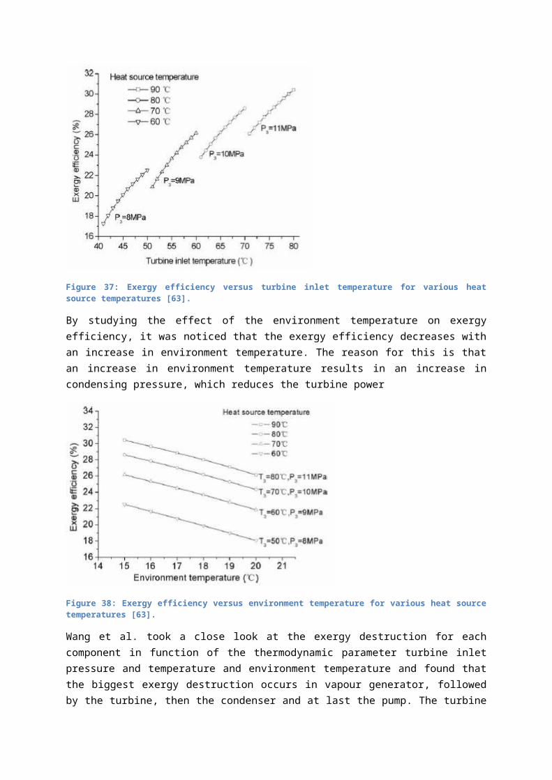
[75] Jackson, J D and Hall, W B, Forced convection heat transfer to fluids at supercritical pressure, Turbulent Forced Convection in Channels and Rod Bundles, 1979, Vol.2, 563-611, published by Hemisphere Publishing Corporation.

[76] Jackson, J D and Hall, W B, Influences of buoyancy on heat transfer to fluids flowing in vertical tubes under turbulent conditions, Turbulent Forced Convection in Channels and Rod Bundles, 1979, Vol2., 613-640, published by Hemisphere Publishing Corporat.

[77] Krasnoshchekov EA, Protopopov VS. Experimental study of heat exchange in carbon dioxide in the supercritical range at high temperature drops. Teplofiz Vys Temp 1966;4:389–98.

[78] Petukhov BS, Kirillov VV. On heat exchange at turbulent flow of liquid in pipes. Teploenergetika 1958;4:63–8.

[79] Song Y, Thermodynamic analysis of a transcritical CO2 power cycle driven by solar energy with liquified natural gas as its heat sink; Applied Energy 92 (2012) 194–203.

[80] Petukhov BS, Krasnoshchekov EA, Protopopov VS. An investigation of heat transfer to fluids flowing in pipes under supercritical conditions. ASME. University of Colorado, Boulder, CO, USA; 1961. p. 569–78.

[81] A. Bejan, Entropy Generation Minimization, CRC Press, Inc., 2004, ISBN 0-8493-9651-4.

[82] J.D. Jackson, W.B. Hall, Influences of buoyancy on heat transfer to fluids flowing in vertical tubes under turbulent conditions. in: S. Kakac, D.B. Spalding (Eds.), Turbulent Forced Convection in Channels and Bundles, vol. 2, 1979, p. 640.

[83] Kyoung-Ho Kang, Soon-Heung Chang. Experimental study on the heat transfer characteristics during the pressure transients under supercritical pressures, International Journal of Heat and Mass Transfer 52 (2009) 4946–4955.

[84] Incropera FP, Dewitt DP. Fundamentals of heat and mass transfer. 5th ed. New York: John Wiley and Sons; 2002.

[85] Cavallini A, Del CD, Doretti L, Longo GA, Rossetto L. Heat transfer and pressure drop during condensation of refrigerants inside horizontal enhanced tubes. Int J Refrig 2000;23:4–25.

[86] Shah MM. A general correlation for heat transfer during film condensation inside pipe. Int J Heat Mass Transfer 1979;22:547–56.

[87] Wang-Touber correlation in Wang H, Touber S. Distributed and non-steady-state modelling of an air cooler. Int J Refrig 1991; 14(2):98–111.

[88] Cheng L, Ribatski G, Thome JR. Analysis of supercritical CO2 cooling in macro and micro-channels. Int J Refrig 2008;31:1301–16.

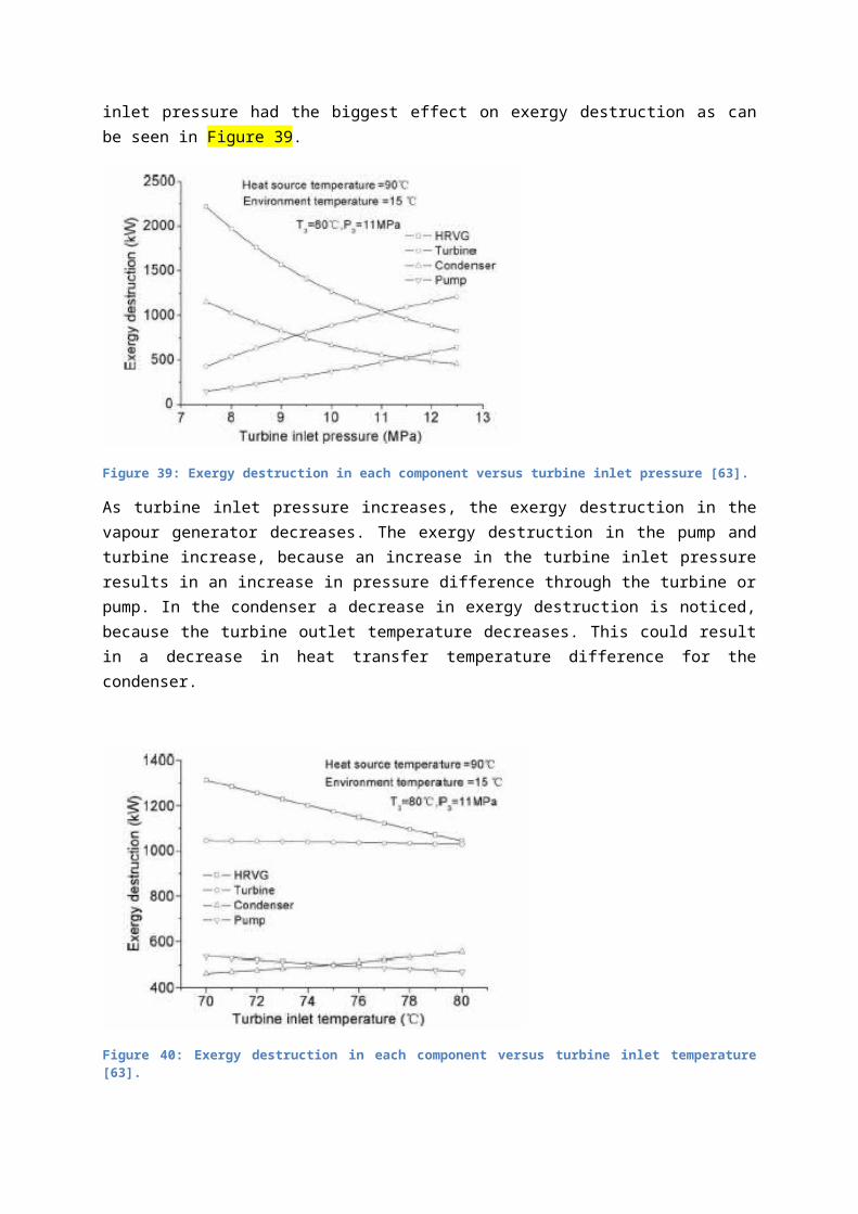
[89] Kyoung-Ho Kang, Soon-Heung Chang. Experimental study on the heat transfer characteristics during the pressure transients under supercritical pressures. Int J Heat Mass Transfer 2009;52:4946–55.

[90] Müller-Steinhagen H, Heck K. A simple pressure drop correlation for twophase flow in pipes. Chem Eng Process 1986;20:297–308.

[91] Collier JG, Thome JR. Convective boiling and condensation. Third ed. Oxford: Clarendon Press; 1994.

[92] Kedzierski MA, Goncalves JM. Horizontal convective condensation of alternative refrigerants within a micro-fin tube. NISTIR 6095. US Dept. Commerce; 1997.