Mutual Fund Performance: Using Bespoke Benchmarks to Disentangle

Mandates, Constraints and Skill

Alessandro Beber, Michael W. Brandt, Jason Cen and Kenneth A. Kavajecz∗

This version: February 2019

Abstract

While no two mutual funds are alike in terms of their mandates and constraints, metrics used to evaluate fund performance relative to peers typically fail to account for these differences by relying on generic benchmark indices and rankings. We develop a methodology to construct a conditional multi-factor benchmark that explicitly incorporates the details of a given fund’s mandates and constraints. The results suggest that (i) mandates and constraints are economically important and affect funds differently, (ii) in general, the average mutual fund has a much improved track record when comparing themselves to a bespoke benchmark, and (iii) the rank ordering of fund bespoke performance relative peers is significantly different than the original rank ordering suggesting investors and regulators would make better decisions regarding their mutual funds if they incorporate the impact of mandates and constraints.

Keywords: mutual funds, performance evaluation, benchmarks, mandates and constraints

JEL classification: G12, G23

∗ Beber is at the Cass Business School, City University London and is also affiliated with CEPR, Brandt is at the Fuqua School of Business, Duke University and is also affiliated with the NBER, Cen is at the University of Essex Business School. We gratefully acknowledge financial support from Inquire Europe. We have benefited greatly from the comments and suggestions of the Inquire Europe Research Committee as well as participants at the 2012 FTSE World Investment Forum. All remaining errors are our own. Please address correspondence to Michael Brandt, Fuqua School of Business, Duke University, 100 Fuqua Drive, Durham, NC 27708 or mbrandt@duke.edu.

2

1. Introduction

It is well-known that market participants rely heavily on rankings relative to peers when

assessing the performance of their mutual funds. Morningstar and Lipper are bellwether

examples of such rankings.1 Traditionally, these performance assessments rank order funds’

returns relative to their chosen benchmark within a defined asset category, e.g. large cap, growth,

etc. There is ample evidence that highly ranked funds attract fund flows (AUM) and low ranked

funds experience redemptions, for example see Del Guercio and Tkac (2008).

Consider that as of 2017, there were over 9,300 U.S. mutual funds controlling $18.7

trillion in total net assets. Moreover, 45.4% of U.S. households hold the overwhelming majority

of those assets as retirement savings via a median of three funds.2 Each quarter these investors

are presented with their funds’ performance relative to a benchmark and peers forming the basis

for either continuing to hold the fund or switch to a competing fund.

In addition, the Investment Company Act of 1940 requires under section 15(c)-3 that the

board of directors/trustees annually review, and if appropriate renew, the contract with the fund

advisor. Key to that review process is the fund’s performance relative to its benchmark and a set

of peers.3 Thus, from a practical/investor and regulatory perspective, the importance of being

1 See https://www.morningstar.com/ and http://www.lipperleaders.com/ 2 Mutual fund statistics taken from the Investment Company Institute Fact Book: https://www.ici.org/pdf/2018_factbook.pdf 3 The Investment Company Act of 1940 mandates that mutual fund Board of Directors annually review and approve the advisory contract. The Fund Directors are specifically asked to consider a number of factors, known as the “Gartenberg factors” after the current precedent setting legal case, when making their determination. Specifically, Directors must consider and evaluate: (1) the nature, extent, and quality of the services provided by the Advisor, including the investment process used by the Advisor; (2) the performance of the Funds in comparison to their benchmark indices and a peer group of mutual funds; (3) the management fees and total operating expenses of the Funds, including comparative information with respect to a peer group of mutual funds; (4) the profitability of the Advisor with respect to the Funds; and (5) the extent to which economies of scale may be realized as the Funds grow.

3

able to properly assess the performance of a mutual fund relative to peers can hardly be

overstated.

A crucial aspect of the appropriateness/accuracy of these rankings is the comparability of

a benchmark and a fund’s performance. A mutual fund’s choice of a benchmark traditionally

utilizes the same asset investment universe (i.e., domestic equities, corporate bonds, international

equities, etc.), and matches the investment size (large, medium, small, micro, etc.) and style (i.e.,

growth, value, momentum, etc.) characteristics. The difference between the fund’s performance

and the benchmark is taken as a measure of performance, or lack thereof. While this

measurement process may make sense for index and absolute return funds, it ignores

fundamental differences between an active mutual fund and benchmark, such as fund mandates

and constraints, which are not imposed on the requisite benchmarks. These mandates and

constraints are made known to investors through their inclusion in the fund’s prospectus,

although internal (non-public) mandates and constraints are being utilized more frequently as of

late.4

As an illustration of the comparability/measurement problem, consider a mutual fund that

has a mandate to invest in small capitalization value stocks, with constraints to be fully invested

at all times and have at least 60% of the portfolio companies be dividend-paying stocks. While a

natural benchmark to use would be the Russell 2000 value index, the percentage of dividend

paying stocks within the index is well below 60%. Moreover, because the Russell 2000 value

index is static, and not subject to a fully-invested budget constraint, it does not need to sell a

4 A Chief Investment Officer (CIO) of a prominent fund family acknowledged that they have a set of externally visible constraints in the prospectus but then impose even tighter constraints on their managers because bumping into official constraints is costly. In addition, internally the fund’s portfolio managers are compensated, not by their performance relative to the public benchmarks, but by their internal benchmark model which is subject to the constraints they impose on each manager to see if they can add alpha through stock selection on top of constraints factor exposure.

4

stock in order to buy another stock and vice versa like the active manager must. As such,

differences between a mutual fund and a benchmark may be the results of mandates, constraints,

skill or a combination of each. Interestingly, the mandates and constraints that are listed within

mutual funds’ prospectuses display substantial heterogeneity; thus, potentially having differential

effects on the performance of funds, and in turn possibly changing the ranking of peer funds.5

Said differently, and the central problem our paper addresses, is that the conventional measure of

fund performance is similar to comparing fruit of all varieties: apples, oranges, strawberries, etc.

Thus, it is important both academically, practically and regulatorily to find a method to make the

comparison/measurement, and subsequent peer ranking, appropriate and meaningful.

Our analysis develops precisely that methodology to account for the mandates and

constraints of a fund manager by adjusting the relevant benchmark to mirror the fund manager’s

mandates and constraints – resulting in an apples-to-apples comparison. The intuition behind

this methodology can be gleaned from taking a simple mean-variance perspective on

performance. Consider a fund of all large capitalization equities over the period 1974-2013,

which has a historical return of 13% and a standard deviation of 20%. Panel A of Chart 1 depicts

the large capitalization equity fund within a standard minimum variance frontier calculation over

the same period. Because the fund is below the Capital Market Line (CML), it delivers less

return, or more risk, than its minimum variance benchmarks. It is standard to interpret the fund

manager as generating negative alpha. It is this interpretation that is inappropriate, given the

substantial differences in mandates and constraints between the fund and the benchmark.

Consider now ‘adjusting’ the minimum-variance frontier to account for the fund specific

5 If all active funds within the same size/style class were subject to the same mandates and constraints, the benchmark comparison would preserve the rank ordering of competing funds.

5

mandates/constraints. Panel B of Chart 1 provides an illustration of how the frontier may be

altered to accommodate the portfolio’s unique set of mandates and constraints. This in turn

alters the interpretation of alpha generation and skill. Thus, the models used as standard

benchmarks, while full of intuition about the trade-off between risk and return, are built upon

many strong assumptions. For example, in the Capital Asset Pricing Model (CAPM), two-fund

separation exists in the presence of full information, simple and clear preferences over only risk

and return, and the absence of practical frictions facing the portfolio manager.

Our results show that once benchmarks are properly adjusted, fund mandates and

constraints display a wide range of effects on both the benchmark returns and manager’s

portfolio choice problem. Specifically, the investment universe (size and style) constraints cost

funds an average excess risk of 190 basis points, with the small and value styles being the most

costly; moreover, cash holdings and leverage add 177 basis points, limits on short-sales adds 80

basis points, and turnover restrictions contribute 141 basis points in average added costs.6 In

addition, the bespoke fund performance results in an average 30 to 40% reduction in fund

manager underperformance with a corresponding increase in the variance of performance. Not

surprisingly, given the heterogeneity in fund mandates and constraints, the bespoke ranking of

peer performance is significantly different than the original ranking, especially for the highest

ranked funds suggesting potentially different investment choices might be made by investors if

armed with the bespoke peer ranking.

Our analysis has important implications for academics and practitioners alike. From an

academic perspective, we provide a flexible methodology to properly compare a fund’s

6 The added costs due to these mandates and constraints are average values across all applicable funds in our sample where the target excess return is 8%.

6

performance to a benchmark. The methodology highlights that while basic asset pricing models

are good at providing intuition regarding risk and return, they are poor at providing an accurate

absolute and relative measurement of the risk/return tradeoff because of their failure to account

for the reality of mandates and constraints.

From the practitioner’s perspective, our results are important for mutual fund investors,

fund advisors/management and fund directors/boards. For mutual fund investors, having a

mechanism to evaluate the performance of a mutual fund, and corresponding rank among peers,

given its unique set of mandates and constraints may be the difference between investing in a

fund that is well-managed within its constraints and investing in a fund that is credited with

performance due its lack of constraints. Similarly, mutual fund advisors/management should be

evaluating portfolio managers based on mandate/constraint adjusted performance for

compensation and retention purposes. Lastly, in order for mutual fund directors/boards to

execute their fiduciary responsibility to their shareholders, they should be comparing the fund

advisor’s performance against an appropriate bespoke benchmark during their annual 15(c)-3

review of the fund’s advisory contract.

The remainder of the paper is organized as follows. Section 2 discusses the related

literature. Section 3 describes our methodology. Section 4 details our sample funds and the

mandates and constraints they face. Section 5 provides model estimates and the costs of

individual and joint mandates and constraints on candidate benchmarks. Section 6 concludes.

7

2. Relevant Literature

Our work is related to three facets of the financial literature: parametric estimation of asset

pricing models, incorporating frictions in asset pricing models, and mutual funds.

The need for parametric estimation arises because the traditional approaches (mean-

variance optimization and factor-mimicking portfolios) are not feasible and flexible enough to

capture fund mandates and constraints. Thus, we adopt the framework of Brandt, Santa-Clara

and Valkanov (2009) for developing a parametric portfolio in which the vector of portfolio

weights is a function of a set of firm characteristic variables. We extend their original

methodology to take account of mandates and constraints, essentially transforming a high-

dimensional constrained portfolio choice problem of individual stocks into a low-dimensional

problem expressed through characteristics.

Researchers have long acknowledged that frictions will deleteriously impact the

performance of asset pricing models. However, the key difference among fund mandates and

constraints and other studied frictions is that mandates and constraints are heterogeneous across

funds, while most other frictions have a homogenous impact within the market place. One

exception, which investigates a single constraint, is Briere and Szafarz (2017). Their

investigation of the impact of short-selling constraints on factor-based portfolios concludes that

accounting for this constraint substantially changes mean-variance performances. The goal of

our paper is to account for the differential impacts of multiple fund constraints and mandates on

fund managers and their respective benchmarks. Given few papers have addressed this issue, we

believe our results make an important contribution to the literature.

The literature on mutual funds is vast, whereby a complete review is beyond the scope of

this paper; however, there are few areas that are relevant to our work: rankings, benchmark

8

choice and retail investor behavior. As mentioned earlier, there is considerable research which

shows the importance and influence that fund rankings have on fund flows and AUM,

representative work includes Blake and Morey (2000) and Del Guercio and Tkac (2008).

A mutual fund’s choice of benchmark is also an important topic. The general consensus from

that literature is that the choice of benchmark has a significant impact on performance,

particularly if there is a mismatch between the investment universes. Sensoy (2009), Mateus,

Mateus and Todorovic (2017), and Cremers, Fulkerson and Riley (2018) suggest that the

benchmark choice may be strategic to bolster performance relative to peers. Finally, our analysis

is related to the behavior of investors in mutual funds. Work by Palmiter (2016) and Freisen and

Nguyen (2018) suggest that retail investors are less than savvy about their investment choices

given they appear ignorant of fund characteristics and unresponsive to risks and fees. Given this

characterization of retail investors, it is not difficult to argue that they would also be unaware of

funds mandates and constraints.

3. Methodology

This section presents a constrained parametric approach to the traditional mean-variance

portfolio choice problem and provides a description of the data, including information on fund

mandates and constraints, which will be used to estimate the model.

3.1 Parametric Benchmark Portfolio Policy

There are numerous ways in which benchmarks are calculated in finance. However, creating the

proper benchmark to account for the differences across fund strategies (mandates, constraints)

requires a parsimonious and feasible procedure for calculation. While mean-variance portfolio

9

optimization may be the first method to spring to mind, it can be quickly dismissed as infeasible,

and in addition, it is well known to be subject to unrealistic portfolio holdings. Similarly, factor-

mimicking portfolios are not a suitable alternative, as it does not provide enough flexibility to

capture the differences underlying various mandates and constraints. Consequently, we utilize a

parametric portfolio approach as in Brandt, Santa-Clara, and Valkanov (2009), which provides

both a feasible and flexible method for calculating bespoke benchmarks. The intuition behind

this approach is similar in spirit to a change in mathematical basis, whereby the variation and

impact of the various constraints and mandates are projected upon fund characteristics rather

than onto a set of portfolio holdings.

Another interpretation of our approach, and one that we will carry through the remainder

of the paper, is that any portfolio that a manager may choose can be decomposed into a set of

beta strategies (long-only portfolios) and a set of alpha strategies (zero-cost hedged portfolios).

The exposures to these strategies are the decision variables in the constrained parametric

portfolio choice problem. In contrast to the traditional mean-variance portfolio choice approach,

which models nonlinear constraints of the high-dimensional space of portfolio weights on

individual assets, our constrained parametric portfolio choice framework specifies fund mandates

and constraints as linear restrictions on a low-dimensional parameter space and the resulting

constrained portfolio choice problem can be easily solved using quadratic programming.

3.2 Econometric Model

Consider an investment universe of N stocks. Each stock belongs to an industry, size, and style

group. Specifically, we consider in our application I = 10 industries based on top level SIC

codes, small and large size groups based on the median firm capitalization, and value and growth

style groups based on the median book-to-market ratio (S = 4 size and style groups). The

10

parametric portfolio approach formulated in Brandt, Santa-Clara and Valkanov (2009)

parameterizes the active portfolio deviations from the market or benchmark portfolio at time t for

stock i as a function of the firm’s observable characteristics, 𝐶𝐶𝑡𝑡,𝑖𝑖.

We adapt the approach of Brandt, Santa-Clara and Valkanov (2009) in three important

ways. The first departure from their approach is to associate each stock separately with (1) the

average characteristics of the industry, size, and style group to which the firm belongs, and (2)

the deviation of the firm’s characteristics from these industry, size, and style group averages.

This modeling choice allows the parametric portfolio to independently tilt into industry, size and

style groups for broad group investments as well as into individual firms within each industry,

size and style group for group-neutral stock investments. We refer to the average characteristics

of the industry, size and style groups as across group characteristics and the firm specific

deviations as within group characteristics.

As in Brandt, Santa-Clara and Valkanov (2009), both sets of characteristics are cross-

sectionally normalized to ensure that portfolio tilts from the market or benchmark portfolio add

up to zero and are not affected by changes in the universe composition such as doubling the

number of firms by simply splitting them up. Specifically, the across group characteristics are

demeaned so that group tilts can be market or benchmark neutral and are scaled by the relative

market capitalization of each firm versus the whole group to ensure that group tilts are market

capitalization weighted. Intuitively, as the portfolio tilts from one group to another, it does so

proportionally more for larger firms within the groups. The within group characteristics are, in

addition to already being demeaned by construction, normalized by the relative market

capitalization of the group versus the whole market. This normalization scales the active

11

investment within each group by the market capitalization of the group instead of the number of

firms within the group.

The second departure from Brandt, Santa-Clara and Valkanov (2009) is that we split both

the across and within group characteristics into positive and negative values with separate

coefficients on each. This allows the portfolio to more aggressively overweight firms with

positive characteristics than underweight firms with equally negative characteristics, or vice

versa. However, by breaking the link between over and under-weights relative to the market or

benchmark portfolio, the active tilts may no longer sum to zero or be self-funded. To

compensate, we introduce another coefficient on the market or benchmark portfolio so that if the

active tilts are net positive (negative) the allocation to the market or benchmark portfolio is

adjusted appropriately less (more) than 100 percent so that the sum of portfolio weights still add

up to one. This is the final modeling departure from Brandt, Santa-Clara and Valkanov (2009).

To summarize, the optimal portfolio weight at time t for stock i, denoted 𝜔𝜔𝑡𝑡,𝑖𝑖, is

parameterized as follows:

𝜔𝜔𝑡𝑡,𝑖𝑖 = 𝛽𝛽0𝜔𝜔�𝑡𝑡,𝑖𝑖 + �̅�𝛽𝑐𝑐�̅�𝑡,𝑖𝑖 + + 𝛽𝛽𝑐𝑐𝑡𝑡,𝑖𝑖

+ + 𝛼𝛼�𝑐𝑐�̅�𝑡,𝑖𝑖 + 𝛼𝛼𝑐𝑐𝑡𝑡,𝑖𝑖 (1)

where 𝜔𝜔�𝑡𝑡,𝑖𝑖 is the weight of the market or benchmark portfolio at time t for stock i, 𝑐𝑐�̅�𝑡,𝑖𝑖 is a vector

of normalized and scaled average characteristics for the industry, size, and style group to which

stock i belongs at time t (the across group characteristics), 𝑐𝑐𝑡𝑡,𝑖𝑖 is a vector of differences between

the firm’s characteristics and the firm’s industry, size, and style group average characteristics

(the within group characteristics). 𝑐𝑐�̅�𝑡,𝑖𝑖 + and 𝑐𝑐𝑡𝑡,𝑖𝑖

+ are vectors that contain the positive values of

across and within group characteristics, respectively, and zeros when the corresponding

characteristics are negative.

12

[𝛽𝛽0, �̅�𝛽,𝛽𝛽,𝛼𝛼�,𝛼𝛼] are the parameters governing the optimal portfolio weights. [𝛼𝛼�,𝛼𝛼] tilt the

portfolio weight symmetrically away from the market or benchmark weight based on the across

and within group characteristics of the firm. These are the zero-cost alpha strategies discussed

in the previous section. [�̅�𝛽,𝛽𝛽] allow this tilt to be asymmetric, where positive (negative) values

create a tilt that overweighs firms with positive (negative) characteristics more than it

underweights firms with equally negative (positive) characteristics. Finally, 𝛽𝛽0 scales the

benchmark weight to allow for tilts that do not sum to zero in the cross-section, or are not self-

funded. The three terms associated with the beta coefficients represent the long-only beta

strategies. To reduce the number of free parameters, we assume that the loadings on the within

across and within group characteristics are the same for all 10 industries. With K characteristics,

this assumption reduces the number of coefficients to 1+16K.7

An alternative interpretation of our parameterization is the common practice of funds

attributing performance relative to the benchmark to “allocation” (across groups) and “selection”

(within groups). “Selection” is that portion of the fund’s return that is due to selecting

outperforming stocks within a sector, while “allocation” is that portion of the return due to being

in outperforming sectors, independent of which stocks were in the fund’s portfolio. In our

parameterization, selection skill comes from non-zero 𝛼𝛼 and 𝛽𝛽 loadings while allocation skill is

due to non-zero 𝛼𝛼� and �̅�𝛽 loadings. In addition, it is common practice for a mutual fund to

impose minimum and maximum allowable deviations from the benchmark weights in the

requisite benchmark portfolio, sometimes called sector/industry bands. These limits would be

corresponding upper constraints on the parametric portfolio parameters.

7 Each of the four size and style groups has two coefficients on K across industry characteristics and two coefficients on K within industry, size and style group characteristics.

13

3.3 Investment universe

We measure the impact of various mandates and constraints relative to the unconditional

minimum variance frontier. Thus, we must define the unconditional investment universe as well

as the size and the style groups. The investment universe includes all traded stocks, except those

whose price is below $5 per share, as well as stocks whose market capitalization is below the

20th percentile in the cross-section. These exclusions are meant to minimize the effect of

extreme observations due to infrequent trading of illiquid securities on our results. We define the

size and style groups based on market capitalization and the book-to-market ratio using NYSE

breakpoints. A stock with a market equity below the 20th percentile is classified as “micro-cap”

(thereby excluded as explained above), between the 20th and 50th percentile (median) as “small

cap”, and above the 50th percentile (median) as “large cap”. Similarly, a firm with a book-to-

market ratio above the 50th percentile (median) is classified as “value” and correspondingly

below as “growth”. Finally, we impose consistency between the investment universe and the

size and style groups in two ways. First, we set the loadings associated with size and style

groups outside the investment universe to zero. Second, we renormalize the market

capitalization weights of all firms in the universe within each size and style group.

3.4 Mandates and Constraints

There are numerous mandates and constraints that obfuscate the measurement of fund

performance relative to a benchmark; thus, a comprehensive investigation of each one is

infeasible. Moreover, fund mandates and constraints display incredible heterogeneity with

respect to how widely they are communicated, the ease/difficulty with which they can be

incorporated into our parametric portfolio problem, and whether they are self-imposed or part of

market-wide financial regulation.

14

To illustrate, consider two examples of mandates and constraints that are imposed by

regulation and difficult to model within our parametric framework. First, the Securities and

Exchange Commission (SEC) requires that once an investor owns five percent or more of the

outstanding shares of a company, they must file a 13G declaring themselves as a large

stakeholder in the company. Furthermore, if the investor has the intention to affect change

within the company through “activism,” they must additionally file a 13D detailing their

intentions and must carefully document any interactions/communications with the company

management going forward. While it is obvious that the benchmark need not file these required

forms as the funds must, what might not be as obvious is how costly compliance with these

regulatory requirements can be. Second, in January 2017 the SEC released a new reporting

mandate, called the “Liquidity Rule,” related to the liquidity profile of the assets held within a

fund. In particular, mutual funds must measure, report and manage the liquidity risk within their

portfolios on a periodic and ongoing basis.8 The imposition of this new regulation has a number

of costs. The fund industry must layer on an additional ongoing regulatory requirement which

will add to the costs of running a fund. Moreover, it will necessarily discourage funds from

owning companies that are classified as illiquid, again placing added costs on the fund managers.

This is certainly not to say that these SEC regulatory requirements are inappropriate or are not

serving an important function, rather they highlight an important set of mandates and constraints

that additionally confound the comparison of the fund and benchmark returns and are difficult to

model without further information.

8 The “Liquidity Rule,” otherwise known as SEC Rule 22e-4 mandates that mutual funds subject to the Investment Company Act of 1940 must review and manage liquidity risk, defined as the risk of not being able to accommodate redemption demand without significant cost, by categorizing investments onto a liquidity spectrum (four categories) and then managing the percentages deemed illiquid. Additional details can be obtained from: https://www.sec.gov/rules/final/2016/33-10233.pdf

15

The mandates and constraints we focus on in this paper are set out in the fund prospectus

or Statement of Additional Information (SAI), are typically chosen by the fund, and are widely

communicated to investors (see Section 4 below for a detailed description of our data).

Specifically, we incorporate five mandates/constraints into our parametric benchmark models:

investment universe, short-sales, borrowing/lending, portfolio turnover and transaction costs, as

these are widely communicated to investors, parsimoniously modeled, and easily interpretable.

3.4.1 Investment universe

It is relatively common for a mutual fund to have a restricted or targeted investment universe

such as growth versus value or large versus medium versus small capitalization firms. Universe

restrictions are simple to impose in our framework by simply redefining and renormalizing the

investment universe in Section 3.3.

3.4.2 Short sales

Some mutual funds are allowed to short-sell to a limited extent. Many funds are prohibited from

short-selling all together. Suppose a fund is allowed to hold a total short position up to q ≥ 0,

then a sufficient condition for this constraint to be satisfied is (𝛼𝛼�,𝛼𝛼)𝚤𝚤2𝐾𝐾𝐾𝐾 ≤ 𝑞𝑞 since the long-short

alpha strategies have a short position by design while the beta strategies are long-only by

construction. Note that this parameter constraint is sufficient and likely overly restrictive, since

some additional allocation to the alpha strategies can be offset by the long holdings of the beta

strategies without producing a total net short position that exceeds the limit.

3.4.3 Borrowing/lending

Cash borrowing and lending constraints essentially place an upper (𝜋𝜋) and lower (𝜋𝜋) bound on

the riskless asset, where 𝜋𝜋 ∈ {0,1] is the cash holding limit and 𝜋𝜋 ≤ 0 is the borrowing limit.

16

Translating these constraints to parameter restrictions obtains: �𝛽𝛽0, �̅�𝛽,𝛽𝛽�𝚤𝚤2𝐾𝐾𝐾𝐾+1 ∈ [1 − 𝜋𝜋, 1 − 𝜋𝜋]

since only the long-only strategies are impacted by borrowing and lending.

3.4.4 Portfolio turnover

A constraint on the extent of trading, or turnover, within the portfolio is modeled by requiring

(monthly) turnover 𝑇𝑇𝑇𝑇(𝑤𝑤) = 𝑬𝑬∑ �Δ𝑤𝑤𝑡𝑡,𝑖𝑖�𝑁𝑁𝑖𝑖=1 to be bounded above by 𝑢𝑢. Given all strategies are

impacted by a constraint on trade, the turnover constraint amounts to the following sufficient

condition in terms of the parameters of the portfolio policy rule:

𝛽𝛽0𝑇𝑇𝑇𝑇(𝑤𝑤�) + �̅�𝛽𝑇𝑇𝑇𝑇(𝑐𝑐̅ +) + 𝛽𝛽𝑇𝑇𝑇𝑇(𝑐𝑐+) + 𝛼𝛼�𝑇𝑇𝑇𝑇(𝑐𝑐̅) + 𝛼𝛼𝑇𝑇𝑇𝑇(𝑐𝑐) ≤ 𝑢𝑢

3.4.5 Transaction costs

Finally, we model transaction costs by adding a function of trades to the objective function of

portfolio return variance:

𝑇𝑇𝐶𝐶 = 12𝜂𝜂Δ𝑤𝑤𝑡𝑡′Σ𝑡𝑡Δ𝑤𝑤𝑡𝑡 ,

where 𝜂𝜂 is a constant which governs the level of trading costs. We calibrate the median level of

this parameter using the following mean-variance criterion:

𝐸𝐸�𝑤𝑤�𝑡𝑡𝑅𝑅𝑡𝑡+1 − 𝑅𝑅𝑓𝑓,𝑡𝑡� − 𝐴𝐴2

[𝐸𝐸(𝑤𝑤𝑡𝑡𝑅𝑅𝑡𝑡+1)2 + �̅�𝜂𝐸𝐸(Δ𝑤𝑤�𝑡𝑡𝑅𝑅𝑡𝑡+1)2] = 0.

This function sets equal the utility of holding a value-weighted market index, which is

rebalanced each month, with the utility of holding cash, given the intensity of transaction cost 𝜂𝜂.

Given standard assumptions, we obtain a medium transaction cost intensity of �̅�𝜂 = 50.9 We also

9 In solving for 𝜂𝜂, we assume that relative risk aversion is A = 5, the equity risk premium is 8%/12 = 0.0067, the variance of the market return is (16%2)/12 = 0.0021, the mean squared variance-adjusted turnover of the value-weighted market index is 1.2 × 10−5.

17

consider two additional liquidity environments, one that is more liquid, where 𝜂𝜂𝑙𝑙𝑙𝑙𝑙𝑙 = 12�̅�𝜂 = 25,

and another that is more illiquid where 𝜂𝜂ℎ𝑖𝑖𝑖𝑖ℎ = 2�̅�𝜂 = 100. The latter liquidity environment

could be interpreted as either fragmented markets, markets with few liquidity providers, or

perhaps periods of market downturns as in 1987, 1997 and 2008.

3.5 Constrained Parametric Portfolio Choice Problem

Combining the basic parametric portfolio problem with the parameterized mandates and

constraints yields the following problem presented here in matrix notation:

min𝜃𝜃�12𝜃𝜃′Ω𝜂𝜂𝜃𝜃� where Ω𝜂𝜂 = 𝐸𝐸[𝑋𝑋𝑡𝑡′𝑅𝑅𝑡𝑡+1𝑒𝑒 𝑅𝑅𝑡𝑡+1

𝑒𝑒′ 𝑋𝑋𝑡𝑡] + 𝜂𝜂𝐸𝐸[Δ𝑋𝑋𝑡𝑡′𝑅𝑅𝑡𝑡+1𝑒𝑒 𝑅𝑅𝑡𝑡+1 𝑒𝑒′ Δ𝑋𝑋𝑡𝑡] (6)

subject to the following constraints:

𝜃𝜃′𝐄𝐄[𝑋𝑋𝑡𝑡′𝑅𝑅𝑡𝑡+1𝑒𝑒 ] = 𝜇𝜇𝑒𝑒 ∶ mean return target

𝜃𝜃′𝒆𝒆𝛼𝛼 ≤ 𝑞𝑞 ∶ short sale

𝜃𝜃′𝒆𝒆𝛽𝛽 ∈ �1 − 𝜋𝜋, 1 − 𝜋𝜋� ∶ borrowing and lending

𝜃𝜃′𝐄𝐄|Δ𝑋𝑋𝑡𝑡′|𝚤𝚤𝑁𝑁 ≤ 𝑢𝑢 ∶ turnover

𝜃𝜃 ≥ 0 ∶ fund level long only

The vectors included in the above problem can be interpreted as follows. The vector 𝒆𝒆𝛽𝛽 selects

only those coefficients that correspond to the long-only strategy, i.e. 𝛽𝛽0, �̅�𝛽, 𝑎𝑎𝑎𝑎𝑎𝑎 𝛽𝛽; therefore, they

are present in the mean return target and borrowing/lending constraint. Correspondingly, the

vector 𝒆𝒆𝛼𝛼 selects those coefficients that pertain to the hedged portfolios, i.e. 𝛼𝛼� 𝑎𝑎𝑎𝑎𝑎𝑎 𝛼𝛼; thereby

only included in the short-sale constraint. Note that any universe constraints are implicit in the

initial dataset construction, and that we added a fund level constraint on the parameters which

should be non-binding as long as firm characteristics are signed appropriately.

18

4. Data

4.1 Market Data

To empirically estimate the parametric model, we require equity returns and accounting data as

well as information regarding mutual fund mandates and constraints. We describe each in turn.

We obtain monthly return, price per share, and shares outstanding of individual U.S. companies

traded in the NYSE, AMEX, and NASDAQ from the Center for Research on Security Prices

(CRSP). We then collect corresponding accounting variables as well as Standard Industry

Classification (SIC) codes from the CRSP-Compustat merged data set. In the case of a missing

SIC code, we complement it using data from CRSP. Stocks are then categorized into 10 industry

sectors based on the definitions outlined on Kenneth French’s Data Library. The sample period

is January 1974 to December 2013.

For each firm, we construct three conditioning characteristic variables: size, or market

equity; value, or book-to-market ratio; and return momentum. Specifically, market equity is

defined as the log of the common share price times the number of common stock shares

outstanding at the end of each June. Book-to-market is measured as the log of the ratio of book

equity measured at the most recent fiscal year-end within the prior calendar year to the market

equity measured at the end of the prior calendar year (December). Finally, momentum is defined

as the one-year return lagged by one month to remove any short-term reversal effects.10

4.2 Fund Mandates and Constraints

10 For a further description of the industry sectors and market variables see Kenneth French’s Data Library website: http://mba.tuck.dartmouth.edu/pages/faculty/ken.french/data_library.html

19

The set of mutual funds we consider are all U.S. equity capital appreciation funds. Our mutual

fund sample choice is based on a singular, clear objective (capital appreciation) as well as a

parsimonious sample of 141 funds, making it feasible to collect the data. For our main analysis

we further narrow the sample to the 71 mutual funds with at least a 10-year track record. In

order to gather the mandate and constraint data for our funds, we reviewed the prospectus for

each one of our sample (capital appreciation) funds. Specifically, we reviewed and hand

collected data from the 485A and 485B Prospectus of Security (POS) as well as the Statement of

Additional Information (SAI) that were submitted to the SEC within, or closest to, the fourth

quarter of 2009.11 In reviewing these prospectuses, we recorded data on 4 dimensions: security

holdings, investment level, other securities, and benchmarks. See Table I for a specific list of

variables coded.

The security holding describes the universe of securities that the fund is constrained to

invest within. Common specifications include growth versus value, large, medium and small

capitalization equities, and foreign holdings, which for most funds were relatively easy to

identify. Investment level refers to the extent that the fund is able to buffer fund flows (in or out)

with borrowing or the ability to hold cash (not be fully invested). The language surrounding the

investment level tends to be broad in order to accommodate infrequent/rare occurrences. For

example, many funds state they have the ability to borrow and hold cash on a “temporary and

defensive basis”, and yet do so only on rare occasions. Other securities captures the extent to

which the fund is able to use derivative contracts as well as taking a short position in securities

and lending securities to other counterparties. Benchmarks are a key piece of information for our

study as it defines the metric by which the fund has chosen to measure its own performance.

11 See http://www.sec.gov/edgar/searchedgar/prospectus.htnm

20

Most funds specify a broad index that is representative of the security holding universe that the

fund is constrained to invest within.

Recall the role of a prospectus is to provide investors accurate information about the

investment strategy, risks, past performance, operations, restrictions, fees and management, so

investors are able to make an informed decision about whether to invest. Not surprisingly, the

ordering of topics, form of presentation and even the language used within these prospectuses

often follows a common template.12 Heuristically, we understand that the generalizations/legal

language within the prospectuses does not always match practice. Moreover, we acknowledge

that some of these mandates and constraints are explicit while others implied. For example,

while a majority of funds have the ability to mitigate fund inflows/outflows, in practice they

maintain a low cash position and borrow little, thereby investing when they receive inflows and

selling when they are redeemed to remain fully invested.

After gathering and reviewing the prospectus mandate and constraint data, we take as the

most relevant constraints to analyze: (1) mandates on the investment universe, (2)

borrowing/lending constraints, (3) short-sale constraints, (4) turnover constraints, and (5)

transaction costs.

Table II presents some summary statistics on the mandates/constraints facing our sample

funds. The sample has a good mix of funds within each of the size/style groups, with

large/growth having the largest number of funds and small/value having the smallest number.

12 For example, see the following links for representative prospectuses within our sample. http://www.sec.gov/Archives/edgar/data/100334/000010033410000014/pea125-2010.htm http://www.sec.gov/Archives/edgar/data/275309/000072921809000035/main.htm

21

Note that some mandates/constraints are rather uniform, for example, cash and short-sale, while

others, like leverage and turnover, have more variation.

5. Properties of Constrained Minimum Variance Frontiers

We perform two estimations of the constrained minimum variance frontiers, one in-sample and

the other out-of-sample; each meant to address a different research question. The in-sample

estimation suits our purpose of ex-post evaluation of fund performance relative to an

appropriately constrained benchmark, while the out-of-sample estimation provides a realistic

estimation of the constrained portfolio using rolling historical data. The out-of-sample

estimation establishes a natural robustness check of the in-sample results with respect to

overfitting the parameters and also provides a window into how real-time, rolling estimation may

impact the mandate and constraint costs.

5.1 In-Sample Portfolio Construction

We present the in-sample results in three complimentary ways. First, we present figures that

show the impact of incorporating individual mandates and constraints on the minimum variance

frontier. Second, we detail the changes to portfolio weights when incorporating mandates and

constraints, and finally, we investigate the impact that mandates and constraints have on

particular investment and trading strategies. In what follows we discuss each in turn.

We begin by addressing the following question: what would be the return variance of a

portfolio constrained to have (i) the same mandates and constraints and, (ii) the same average

return as the fund in consideration? To this end, we estimate the parameters of the constrained

portfolio, theta, for any given value of mean excess return using the full-sample of

22

data/information. We then construct the constrained portfolio based on the point estimates of

parameters, 𝜃𝜃�𝐼𝐼𝑁𝑁.

Charts 2-5 display the effects of the various mandates and constraints on the minimum

variance frontier. Intuitively, the constrained minimum variance frontiers tend to be located

inside (less return and more risk) the unconstrained or less constrained frontiers. The following

analysis addresses each mandate/constraint individually.

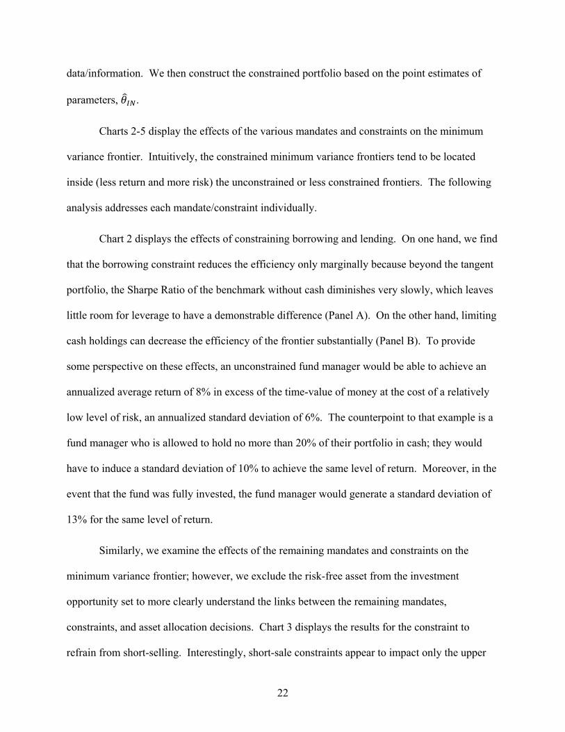
Chart 2 displays the effects of constraining borrowing and lending. On one hand, we find

that the borrowing constraint reduces the efficiency only marginally because beyond the tangent

portfolio, the Sharpe Ratio of the benchmark without cash diminishes very slowly, which leaves

little room for leverage to have a demonstrable difference (Panel A). On the other hand, limiting

cash holdings can decrease the efficiency of the frontier substantially (Panel B). To provide

some perspective on these effects, an unconstrained fund manager would be able to achieve an

annualized average return of 8% in excess of the time-value of money at the cost of a relatively

low level of risk, an annualized standard deviation of 6%. The counterpoint to that example is a

fund manager who is allowed to hold no more than 20% of their portfolio in cash; they would

have to induce a standard deviation of 10% to achieve the same level of return. Moreover, in the

event that the fund was fully invested, the fund manager would generate a standard deviation of

13% for the same level of return.

Similarly, we examine the effects of the remaining mandates and constraints on the

minimum variance frontier; however, we exclude the risk-free asset from the investment

opportunity set to more clearly understand the links between the remaining mandates,

constraints, and asset allocation decisions. Chart 3 displays the results for the constraint to

refrain from short-selling. Interestingly, short-sale constraints appear to impact only the upper

23

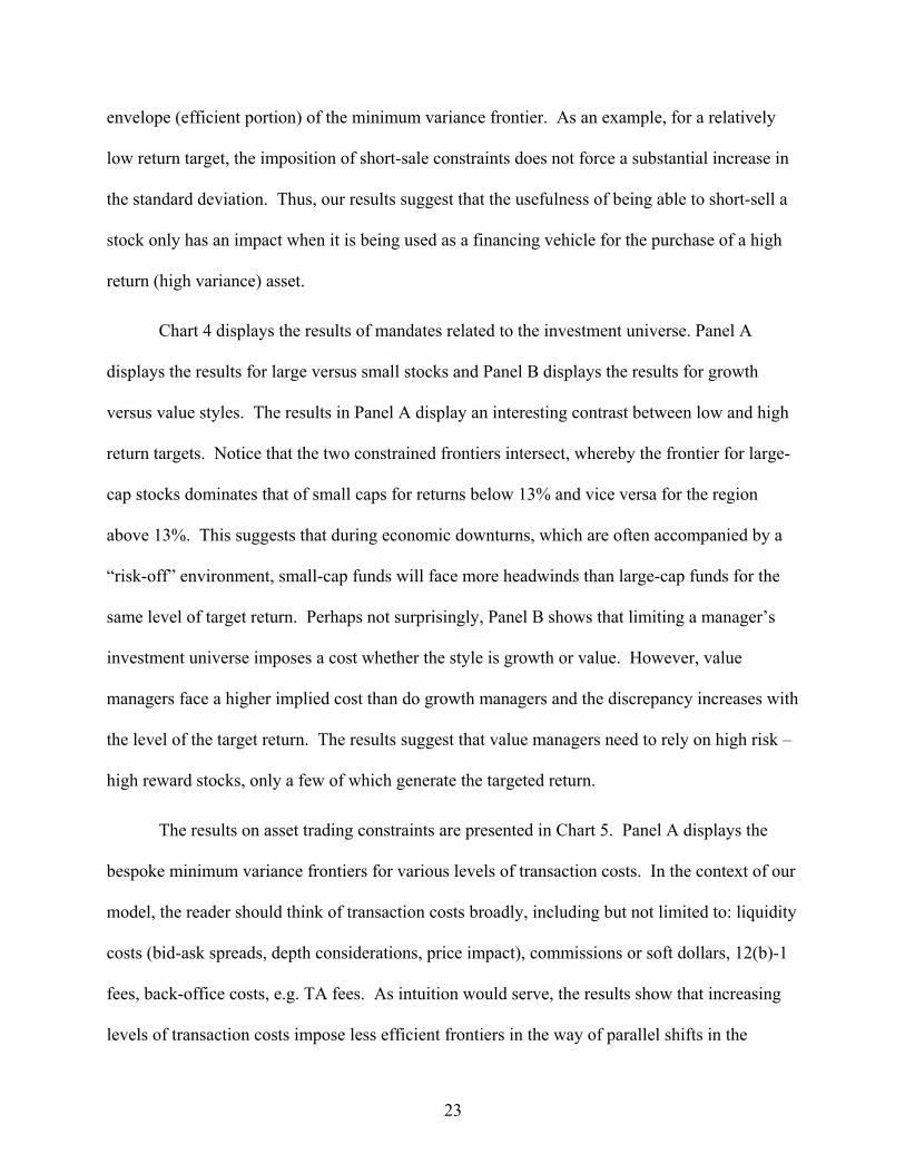
envelope (efficient portion) of the minimum variance frontier. As an example, for a relatively

low return target, the imposition of short-sale constraints does not force a substantial increase in

the standard deviation. Thus, our results suggest that the usefulness of being able to short-sell a

stock only has an impact when it is being used as a financing vehicle for the purchase of a high

return (high variance) asset.

Chart 4 displays the results of mandates related to the investment universe. Panel A

displays the results for large versus small stocks and Panel B displays the results for growth

versus value styles. The results in Panel A display an interesting contrast between low and high

return targets. Notice that the two constrained frontiers intersect, whereby the frontier for large-

cap stocks dominates that of small caps for returns below 13% and vice versa for the region

above 13%. This suggests that during economic downturns, which are often accompanied by a

“risk-off” environment, small-cap funds will face more headwinds than large-cap funds for the

same level of target return. Perhaps not surprisingly, Panel B shows that limiting a manager’s

investment universe imposes a cost whether the style is growth or value. However, value

managers face a higher implied cost than do growth managers and the discrepancy increases with

the level of the target return. The results suggest that value managers need to rely on high risk –

high reward stocks, only a few of which generate the targeted return.

The results on asset trading constraints are presented in Chart 5. Panel A displays the

bespoke minimum variance frontiers for various levels of transaction costs. In the context of our

model, the reader should think of transaction costs broadly, including but not limited to: liquidity

costs (bid-ask spreads, depth considerations, price impact), commissions or soft dollars, 12(b)-1

fees, back-office costs, e.g. TA fees. As intuition would serve, the results show that increasing

levels of transaction costs impose less efficient frontiers in the way of parallel shifts in the

24

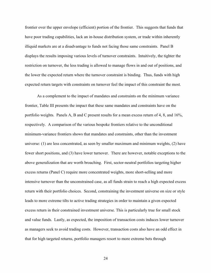
frontier over the upper envelope (efficient) portion of the frontier. This suggests that funds that

have poor trading capabilities, lack an in-house distribution system, or trade within inherently

illiquid markets are at a disadvantage to funds not facing those same constraints. Panel B

displays the results imposing various levels of turnover constraints. Intuitively, the tighter the

restriction on turnover, the less trading is allowed to manage flows in and out of positions, and

the lower the expected return where the turnover constraint is binding. Thus, funds with high

expected return targets with constraints on turnover feel the impact of this constraint the most.

As a complement to the impact of mandates and constraints on the minimum variance

frontier, Table III presents the impact that these same mandates and constraints have on the

portfolio weights. Panels A, B and C present results for a mean excess return of 4, 8, and 16%,

respectively. A comparison of the various bespoke frontiers relative to the unconditional

minimum-variance frontiers shows that mandates and constraints, other than the investment

universe: (1) are less concentrated, as seen by smaller maximum and minimum weights, (2) have

fewer short positions, and (3) have lower turnover. There are however, notable exceptions to the

above generalization that are worth broaching. First, sector-neutral portfolios targeting higher

excess returns (Panel C) require more concentrated weights, more short-selling and more

intensive turnover than the unconstrained case, as all funds strain to reach a high expected excess

return with their portfolio choices. Second, constraining the investment universe on size or style

leads to more extreme tilts to active trading strategies in order to maintain a given expected

excess return in their constrained investment universe. This is particularly true for small stock

and value funds. Lastly, as expected, the imposition of transaction costs induces lower turnover

as managers seek to avoid trading costs. However, transaction costs also have an odd effect in

that for high targeted returns, portfolio managers resort to more extreme bets through

25

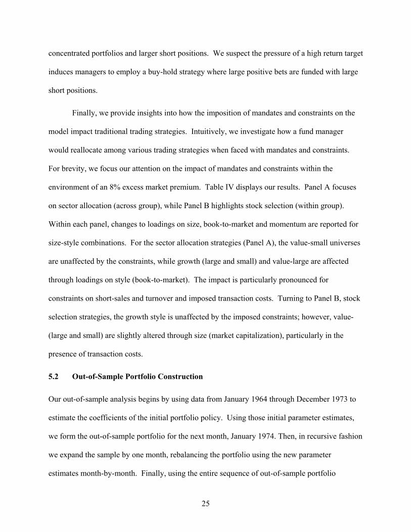
concentrated portfolios and larger short positions. We suspect the pressure of a high return target

induces managers to employ a buy-hold strategy where large positive bets are funded with large

short positions.

Finally, we provide insights into how the imposition of mandates and constraints on the

model impact traditional trading strategies. Intuitively, we investigate how a fund manager

would reallocate among various trading strategies when faced with mandates and constraints.

For brevity, we focus our attention on the impact of mandates and constraints within the

environment of an 8% excess market premium. Table IV displays our results. Panel A focuses

on sector allocation (across group), while Panel B highlights stock selection (within group).

Within each panel, changes to loadings on size, book-to-market and momentum are reported for

size-style combinations. For the sector allocation strategies (Panel A), the value-small universes

are unaffected by the constraints, while growth (large and small) and value-large are affected

through loadings on style (book-to-market). The impact is particularly pronounced for

constraints on short-sales and turnover and imposed transaction costs. Turning to Panel B, stock

selection strategies, the growth style is unaffected by the imposed constraints; however, value-

(large and small) are slightly altered through size (market capitalization), particularly in the

presence of transaction costs.

5.2 Out-of-Sample Portfolio Construction

Our out-of-sample analysis begins by using data from January 1964 through December 1973 to

estimate the coefficients of the initial portfolio policy. Using those initial parameter estimates,

we form the out-of-sample portfolio for the next month, January 1974. Then, in recursive fashion

we expand the sample by one month, rebalancing the portfolio using the new parameter

estimates month-by-month. Finally, using the entire sequence of out-of-sample portfolio

26

estimates, we recalculate the relative performance of our sample capital appreciation funds

against their respective bespoke benchmarks, over a 3, 5, and 10-year horizon as is feasible given

the tenure of our sample funds.

As a robustness check, we analyze the correlation of returns between the in- and out-of-

sample benchmark portfolios without cash for a spread of excess return targets. The out-of-

sample portfolios are highly correlated with the in-sample portfolios, where the correlation for

4% excess return is 0.97 and drops monotonically to 0.93 at an excess return of 32%. Therefore,

we are confident in both the model specifications and the ability to utilize a rolling portfolio

rebalancing to investigate the impact of mandates and constraints. In addition, Chart 6 compares

the performance of the in-sample and out-of-sample benchmarks on standard deviation of

returns, average excess return, and the Sharpe ratio in Panels A, B and C, respectively. The

standard deviation estimates are very similar, suggesting an even spread of return variation over

time where the in-sample estimates provide lower standard deviations below 25%. In contrast,

the average excess return between the two sets of estimates diverges sharply above the inflection

point of 12%, with the in-sample estimates, perhaps not surprisingly, providing higher average

excess returns. Finally, combining these two sets of results, we learn from the Sharpe Ratio

results in Panel C that the two sets of estimates are similar for reasonable excess return targets,

but diverge above a target of 20% where the out-of-sample portfolio deliver a maximum Sharpe

ratio of 1.0 compared to 1.2 for the in-sample portfolio. Thus, in general, the relatively small

difference between the performance of the two sets of portfolios over reasonable excess return

targets lends strong support to our model and its specification.

5.3 Measuring Mutual Fund Performance and Rank

27

In this section, we analyze an essential question. If fund benchmarks were properly adjusted to

account for mandates and constraints facing the funds, thus, allowing an apples-to-apples

comparison — how would this impact the distribution and rank of relative performance of

mutual funds? Said differently, how is the cross-section of relative fund performance altered, if

at all, when properly accounting for mandates and constraints?

We illustrate our procedure of building the requisite bespoke skill distribution by first

providing two single fund examples to highlight how we account for individual mandates and

constraints. Specifically, we use the Value Line Large Companies Fund and the Janus

Investment Fund as our examples because they span the entire sample period (January 1974 to

December 2013) and they both face a broad set of mandates and constraints. The Value Line

Fund is a large-cap fund with December 2013 AUM of $0.21B and the S&P 500 as its chosen

benchmark; the Janus Fund is a value fund with December 2013 AUM of $1.75B and the FTSE

EPRA/NAREIT Developed and Global Indices as its chosen benchmark.

We begin by considering the unconstrained benchmark coupled with the risk-free asset,

then we sequentially account for mandates and constraints, adding a single additional constraint

in each successive step. Because the contribution of each constraint to the shift in the minimum

variance frontier is not independent, we fix the order that constraints will be addressed.

Specifically, the constraint ordering we employ is: investment universe, borrowing/lending,

short-sale, turnover, and transaction costs.13

Chart 7 illustrates how mandates and constraints are incorporated to sequentially create

the bespoke benchmarks, Panel A displays the Value Line Fund and Panel B displays the Janus

13 We perform robustness checks on the ordering of our mandates and constraints, and while the estimates vary slightly, the results are both quantitatively and qualitatively similar and are available upon request.

28

Investment fund. A number of interesting results emerge from this simple comparison. First, the

impact of mandates and constraints can be very different across individual funds. For example,

consider the mandate to be fully-invested with a zero-cash balance (the second adjustment from

the benchmark). The adjustment for the Janus Investment Fund is much larger than the

adjustment for the Value Line Large Companies Fund, likely due to the more illiquid nature of

value stocks. Second, if the difference between the standard deviations of a benchmark and the

two sample funds is smaller, then we observe that this difference relative to the bespoke

benchmark adjusted for mandates and constraints is higher in both cases. Lastly, the

performances of the two funds diverge from each other (namely, have a wider spread) after

adjusting for mandates and constraints. Relative to the unconstrained benchmark, the fund

performances are -13% and -11%, respectively (200 basis point difference), while relative to the

bespoke constrained benchmark the performances are -6.1% and -2.7% (340 basis points

difference), respectively.

With our two examples as a backdrop, we turn our attention to constructing the full

sample distribution of bespoke performance levels and fund rankings. Note that to be included

in this analysis we require our sample funds to have a minimum of 10 years of data. We adopt

this investment horizon screen to focus attention on fund performance over the long-run. This

screen results in 71 funds with which we repeat the process applied to the example funds above,

namely, we estimate the parameters of the unconstrained and constrained portfolio policies by

matching the time-series of the fund return and the market data.

To facilitate our assessment of fund performance, we define two comparison metrics.

The first is excess risk defined as 𝜎𝜎𝑖𝑖 − 𝜎𝜎𝑏𝑏, where 𝜎𝜎𝑖𝑖 is the standard deviation of fund 𝑖𝑖’s excess

returns and 𝜎𝜎𝑏𝑏 is the standard deviation of the benchmark portfolio’s excess returns. The second

29

is the return-adjusted excess risk defined as 𝜎𝜎𝑖𝑖−𝜎𝜎𝑏𝑏𝜇𝜇𝑖𝑖

, where the numerator is the excess risk metric

defined above and 𝜇𝜇𝑖𝑖 is the mean excess return of fund 𝑖𝑖. The return-adjusted excess risk

effectively measures the excessive risk per unit of expected excess return and can be interpreted

as the additional risk the fund manager needs to take for each percentage point of expected

excess return earned by the fund.14

Our fund performance results are presented in Chart 8 and Table V. Chart 8 displays the

distribution of return-adjusted excess risk measured against the original and bespoke benchmarks

and Table V displays the associated statistical comparisons between the two distributions. Chart

8 shows a dramatic shift in the distribution of return-adjusted excess risk toward zero, suggesting

far less under-performance relative to their bespoke benchmarks than implied by the original

benchmarks. Table V compares the moments of the two distributions. The results show a

monotonic and statistically significant reduction in fund underperformance (mean) for both

metrics with the inclusion of each additional mandate and constraint. In addition, the standard

deviation of both metrics tends to increase with each added mandate and constraint, which

suggests more of a performance discrepancy between funds than was previous appreciated.

Skewness and kurtosis are more ambiguous, although there appears to be less skewness and

kurtosis for the bespoke distribution of return-adjusted excess risk.

As the distribution of fund performance is altered with bespoke benchmarks, is it natural

to hypothesize that the relative rank of funds would also change. Chart 9 displays the bespoke

performance rankings and those rankings based on traditional performance for our sample of 71

14 We present the differences in terms of risk, instead of the more common return (alpha) approach, for two reasons. First, changing the minimum-variance optimization to maximize return given risk poses an estimation challenge in that it penalizes highly constrained portfolios (e.g., no leverage, no short-sale, low turnover) to achieve a high risk target. Second, comparisons of Sharpe Ratios are also problematic, as managers with higher target return would be labelled as less skilled.

30

funds partitioned into the four fund subgroups, large, small, growth and value, in panels A

through D, respectively. As above, performance is measured as return-adjusted excess risk.15

The chart is constructed so the diagonal represents the original rankings of funds and the vertical

bars represent the bespoke rankings; thus, bars above (below) the diagonal represent a rank

improvement (deterioration) with the bespoke benchmark. The results include a number of

noteworthy observations. First, the bespoke rankings are statistically different for all subgroups.

In particular, tests of the equality of matched pairs of observations using the Wilcoxon matched-

pairs signed-ranks test can be rejected at the 1% level for each group. Second, of the four

groups, the large-capitalization funds display the least change in the rankings, likely because the

stock universe is small and liquidity ample relative to the other groups. Third, ranking changes

appear to be concentrated at the top of the rankings (best) rather than at the bottom, perhaps

because the performance differential among funds is decreasing with rank. In particular, there is

substantial change in the rank of the top three funds for small, growth and value, with the highest

ranked fund changing for small and value. As an example, consider the value group in Panel D.

The top two funds in the original ranking were the Third Avenue Value Fund ($2.55B AUM,

MSCI World Index as benchmark) and the Franklin Balance Sheet Investment Fund ($1.72B

AUM, Russell 3000 Value Index as benchmark), respectively. After taking account of individual

fund mandates and constraints, the Third Avenue Value Fund falls to third, the Franklin Balance

Sheet Investment Fund remains second and the Gabelli Value Fund ($0.64B AUM with S&P500

as benchmark) takes over the top-ranked spot moving up from fourth place. Thus, value

15 While rankings based on risk-adjusted returns are theoretically appropriate, we acknowledge that market participants traditionally measure performance rank as a simple return difference between the fund and respective benchmark. As a robustness check we have compared the simple return differential rank with the bespoke rank and the results are both quantitatively and qualitatively similar to those shown.

31

investors would likely have reallocated assets in the Gabelli Value Fund had they been informed

of the fund performance rank relative to the bespoke benchmark.

6. Conclusion

We develop a methodology to incorporate frictions into financial settings where heretofore their

impact could not be quantified. We apply our methodology to the lingering academic quandary

regarding the appropriateness of comparing mutual fund performance to a benchmark that does

not share the same mandates and constraints. The approach utilizes a parametric re-mapping of

portfolio weights having imposed individual fund mandates and constraints. Our results

demonstrate that fund mandates and constraints are pervasive and impose costs on funds that are

economically important. Consistent with their importance, they impact both fund portfolio

weights and manager trading strategies.

By constructing bespoke benchmarks for a sample of mutual funds, we are also able to

improve on performance evaluation of mutual funds and their relative ranking. A comparison of

fund performance relative to its appropriate bespoke benchmark within our sample shows a

monotonic increase in relative performance with the inclusion of each additional mandate and

constraint, where the aggregate increase is between 30 and 40%. More important than the

increase in relative performance is the change in the ranking of peer funds. Performance

rankings that account for fund mandates and constraints are significantly and economically

different than traditional rankings which fail to do so. Funds investing in small-cap, growth and

value display the largest ranking changes, particularly for the top ranked funds. Armed with

these bespoke rankings, investors and board members would likely make different investment

decisions suggesting an improved allocation of capital and oversight among mutual funds.

32

References

Blake, C. and M. Morey, 2000, Morningstar Ratings and Mutual Fund Performance, Journal of Financial and Quantitative Analysis 35, 451-483.

Brandt, M., P. Santa-Clara and R. Valkanov, 2009, Parametric Portfolio Policies: Exploiting Characteristics in the Cross-Section of Equity Returns, Review of Financial Studies 22, 3411-3447.

Briere, M. and A. Szafarz, 2017, Factor Investing: The Rocky Road from Long Only to Long Short in Factor Investing, Edited by E. Jurczenko, ISTE Press Ltd.

Cremers, M., J. Fulkerson, and T. Riley, 2018, Benchmark Discrepancies and Mutual Fund Performance Evaluation, University of Notre Dame, Working Paper.

Del Guercio, D., and P. Tkac, 2008, Star Power: The Effect of Morningstar Ratings on Mutual Fund Flow, Journal of Financial and Quantitative Analysis 43, 907-936.

Friesen, G. and V. Nguyen, 2018, The Economic Impact of Mutual Fund Investor Behaviors, University of Nebraska, Working Paper.

Investment Company Institute, 2018, Fact Book. Mateus, I., C. Mateus and N. Todorovic, 2017, The Impact of Benchmark Choice on US Mutual

Fund Benchmark-Adjusted Performance and Ranking, University of Greenwich, Working Paper.

Palmiter, A., 2016, The Mutual Fund Investor, Elgar Handbook of Mutual Fund Regulation, Forthcoming.

Sensoy, B., 2009, Performance Evaluation and Self-designated Benchmark Indexes in the Mutual Fund Industry, Journal of Financial Economics 92, 25-39.

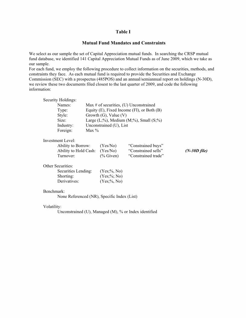
Table I

Mutual Fund Mandates and Constraints

We select as our sample the set of Capital Appreciation mutual funds. In searching the CRSP mutual fund database, we identified 141 Capital Appreciation Mutual Funds as of June 2009, which we take as our sample. For each fund, we employ the following procedure to collect information on the securities, methods, and constraints they face. As each mutual fund is required to provide the Securities and Exchange Commission (SEC) with a prospectus (485POS) and an annual/semiannual report on holdings (N-30D), we review these two documents filed closest to the last quarter of 2009, and code the following information:

Security Holdings: Names: Max # of securities, (U) Unconstrained

Type: Equity (E), Fixed Income (FI), or Both (B) Style: Growth (G), Value (V) Size: Large (L;%), Medium (M;%), Small (S;%) Industry: Unconstrained (U), List Foreign: Max %

Investment Level: Ability to Borrow: (Yes/No) “Constrained buys” Ability to Hold Cash: (Yes/No) “Constrained sells” (N-30D file) Turnover: (% Given) “Constrained trade”

Other Securities: Securities Lending: (Yes;%, No)

Shorting: (Yes;%; No) Derivatives: (Yes;%, No)

Benchmark: None Referenced (NR), Specific Index (List)

Volatility: Unconstrained (U), Managed (M), % or Index identified

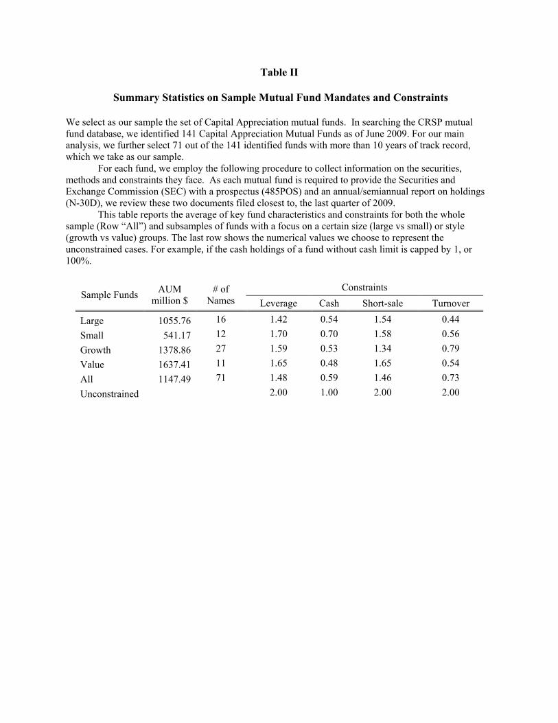
Table II

Summary Statistics on Sample Mutual Fund Mandates and Constraints

We select as our sample the set of Capital Appreciation mutual funds. In searching the CRSP mutual fund database, we identified 141 Capital Appreciation Mutual Funds as of June 2009. For our main analysis, we further select 71 out of the 141 identified funds with more than 10 years of track record, which we take as our sample.

For each fund, we employ the following procedure to collect information on the securities, methods and constraints they face. As each mutual fund is required to provide the Securities and Exchange Commission (SEC) with a prospectus (485POS) and an annual/semiannual report on holdings (N-30D), we review these two documents filed closest to, the last quarter of 2009.

This table reports the average of key fund characteristics and constraints for both the whole sample (Row “All”) and subsamples of funds with a focus on a certain size (large vs small) or style (growth vs value) groups. The last row shows the numerical values we choose to represent the unconstrained cases. For example, if the cash holdings of a fund without cash limit is capped by 1, or 100%.

Sample Funds AUM million $

# of Names

Constraints Leverage Cash Short-sale Turnover

Large 1055.76 16 1.42 0.54 1.54 0.44 Small 541.17 12 1.70 0.70 1.58 0.56 Growth 1378.86 27 1.59 0.53 1.34 0.79 Value 1637.41 11 1.65 0.48 1.65 0.54 All 1147.49 71 1.48 0.59 1.46 0.73 Unconstrained 2.00 1.00 2.00 2.00

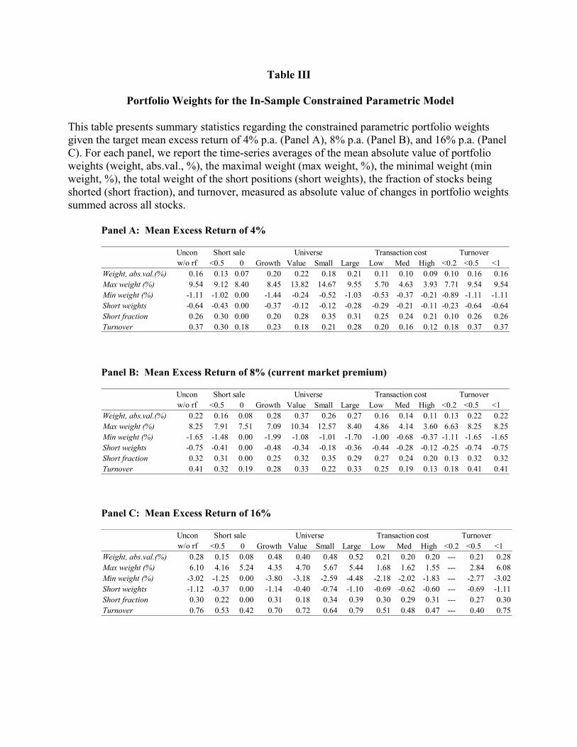
Table III

Portfolio Weights for the In-Sample Constrained Parametric Model This table presents summary statistics regarding the constrained parametric portfolio weights given the target mean excess return of 4% p.a. (Panel A), 8% p.a. (Panel B), and 16% p.a. (Panel C). For each panel, we report the time-series averages of the mean absolute value of portfolio weights (weight, abs.val., %), the maximal weight (max weight, %), the minimal weight (min weight, %), the total weight of the short positions (short weights), the fraction of stocks being shorted (short fraction), and turnover, measured as absolute value of changes in portfolio weights summed across all stocks.

Panel A: Mean Excess Return of 4%

Panel B: Mean Excess Return of 8% (current market premium)

Panel C: Mean Excess Return of 16%

<0.5 0 Growth Value Small Large Low Med High <0.2 <0.5 <1Weight, abs.val.(%) 0.16 0.13 0.07 0.20 0.22 0.18 0.21 0.11 0.10 0.09 0.10 0.16 0.16Max weight (%) 9.54 9.12 8.40 8.45 13.82 14.67 9.55 5.70 4.63 3.93 7.71 9.54 9.54Min weight (%) -1.11 -1.02 0.00 -1.44 -0.24 -0.52 -1.03 -0.53 -0.37 -0.21 -0.89 -1.11 -1.11Short weights -0.64 -0.43 0.00 -0.37 -0.12 -0.12 -0.28 -0.29 -0.21 -0.11 -0.23 -0.64 -0.64Short fraction 0.26 0.30 0.00 0.20 0.28 0.35 0.31 0.25 0.24 0.21 0.10 0.26 0.26Turnover 0.37 0.30 0.18 0.23 0.18 0.21 0.28 0.20 0.16 0.12 0.18 0.37 0.37

Uncon w/o rf

Short sale Universe Transaction cost Turnover

<0.5 0 Growth Value Small Large Low Med High <0.2 <0.5 <1Weight, abs.val.(%) 0.22 0.16 0.08 0.28 0.37 0.26 0.27 0.16 0.14 0.11 0.13 0.22 0.22Max weight (%) 8.25 7.91 7.51 7.09 10.34 12.57 8.40 4.86 4.14 3.60 6.63 8.25 8.25Min weight (%) -1.65 -1.48 0.00 -1.99 -1.08 -1.01 -1.70 -1.00 -0.68 -0.37 -1.11 -1.65 -1.65Short weights -0.75 -0.41 0.00 -0.48 -0.34 -0.18 -0.36 -0.44 -0.28 -0.12 -0.25 -0.74 -0.75Short fraction 0.32 0.31 0.00 0.25 0.32 0.35 0.29 0.27 0.24 0.20 0.13 0.32 0.32Turnover 0.41 0.32 0.19 0.28 0.33 0.22 0.33 0.25 0.19 0.13 0.18 0.41 0.41

Uncon w/o rf

Short sale Universe Transaction cost Turnover

<0.5 0 Growth Value Small Large Low Med High <0.2 <0.5 <1Weight, abs.val.(%) 0.28 0.15 0.08 0.48 0.40 0.48 0.52 0.21 0.20 0.20 --- 0.21 0.28Max weight (%) 6.10 4.16 5.24 4.35 4.70 5.67 5.44 1.68 1.62 1.55 --- 2.84 6.08Min weight (%) -3.02 -1.25 0.00 -3.80 -3.18 -2.59 -4.48 -2.18 -2.02 -1.83 --- -2.77 -3.02Short weights -1.12 -0.37 0.00 -1.14 -0.40 -0.74 -1.10 -0.69 -0.62 -0.60 --- -0.69 -1.11Short fraction 0.30 0.22 0.00 0.31 0.18 0.34 0.39 0.30 0.29 0.31 --- 0.27 0.30Turnover 0.76 0.53 0.42 0.70 0.72 0.64 0.79 0.51 0.48 0.47 --- 0.40 0.75

Uncon w/o rf

Short sale Universe Transaction cost Turnover

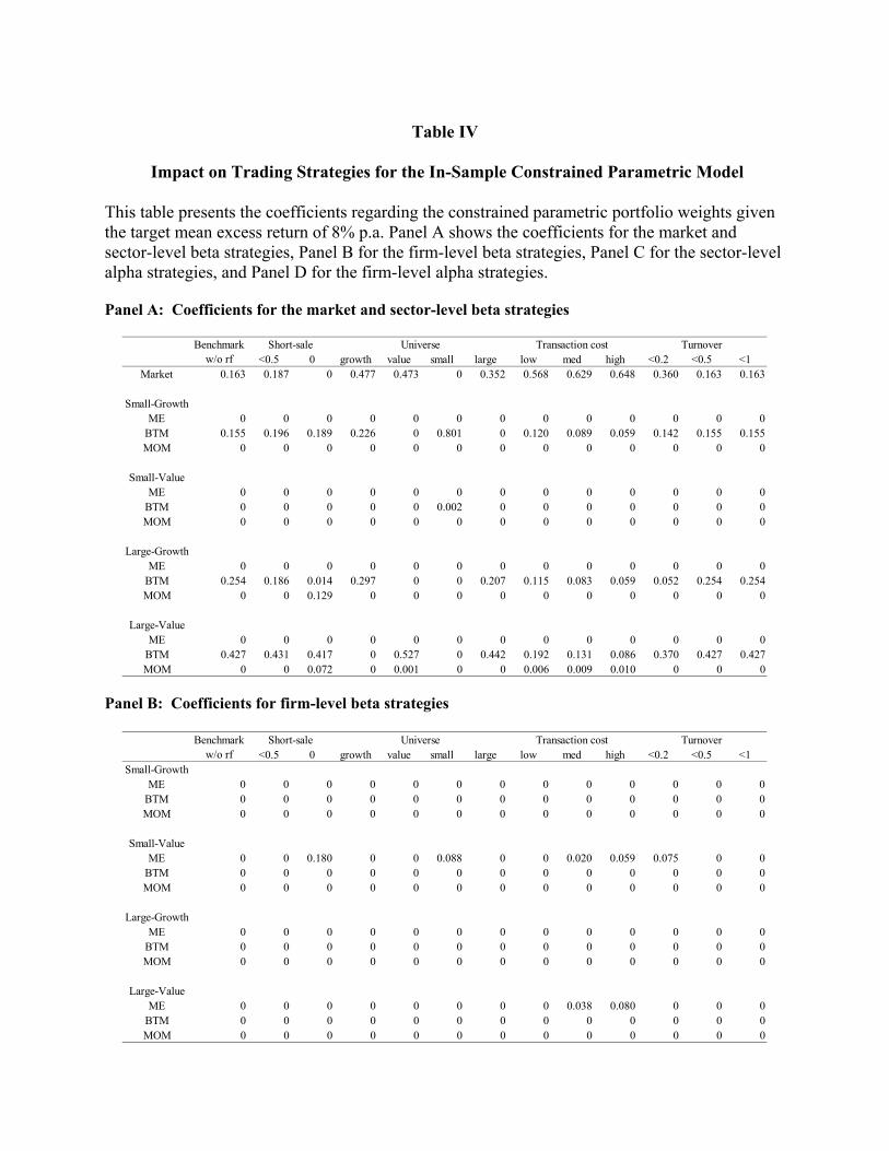
Table IV

Impact on Trading Strategies for the In-Sample Constrained Parametric Model

This table presents the coefficients regarding the constrained parametric portfolio weights given the target mean excess return of 8% p.a. Panel A shows the coefficients for the market and sector-level beta strategies, Panel B for the firm-level beta strategies, Panel C for the sector-level alpha strategies, and Panel D for the firm-level alpha strategies. Panel A: Coefficients for the market and sector-level beta strategies

Panel B: Coefficients for firm-level beta strategies

<0.5 0 growth value small large low med high <0.2 <0.5 <1Market 0.163 0.187 0 0.477 0.473 0 0.352 0.568 0.629 0.648 0.360 0.163 0.163

Small-GrowthME 0 0 0 0 0 0 0 0 0 0 0 0 0

BTM 0.155 0.196 0.189 0.226 0 0.801 0 0.120 0.089 0.059 0.142 0.155 0.155MOM 0 0 0 0 0 0 0 0 0 0 0 0 0

Small-ValueME 0 0 0 0 0 0 0 0 0 0 0 0 0

BTM 0 0 0 0 0 0.002 0 0 0 0 0 0 0MOM 0 0 0 0 0 0 0 0 0 0 0 0 0

Large-GrowthME 0 0 0 0 0 0 0 0 0 0 0 0 0

BTM 0.254 0.186 0.014 0.297 0 0 0.207 0.115 0.083 0.059 0.052 0.254 0.254MOM 0 0 0.129 0 0 0 0 0 0 0 0 0 0

Large-ValueME 0 0 0 0 0 0 0 0 0 0 0 0 0

BTM 0.427 0.431 0.417 0 0.527 0 0.442 0.192 0.131 0.086 0.370 0.427 0.427MOM 0 0 0.072 0 0.001 0 0 0.006 0.009 0.010 0 0 0

Benchmark w/o rf

Short-sale Universe Transaction cost Turnover

<0.5 0 growth value small large low med high <0.2 <0.5 <1Small-Growth

ME 0 0 0 0 0 0 0 0 0 0 0 0 0BTM 0 0 0 0 0 0 0 0 0 0 0 0 0MOM 0 0 0 0 0 0 0 0 0 0 0 0 0

Small-ValueME 0 0 0.180 0 0 0.088 0 0 0.020 0.059 0.075 0 0

BTM 0 0 0 0 0 0 0 0 0 0 0 0 0MOM 0 0 0 0 0 0 0 0 0 0 0 0 0

Large-GrowthME 0 0 0 0 0 0 0 0 0 0 0 0 0

BTM 0 0 0 0 0 0 0 0 0 0 0 0 0MOM 0 0 0 0 0 0 0 0 0 0 0 0 0

Large-ValueME 0 0 0 0 0 0 0 0 0.038 0.080 0 0 0

BTM 0 0 0 0 0 0 0 0 0 0 0 0 0MOM 0 0 0 0 0 0 0 0 0 0 0 0 0

Benchmark w/o rf

Short-sale Universe Transaction cost Turnover

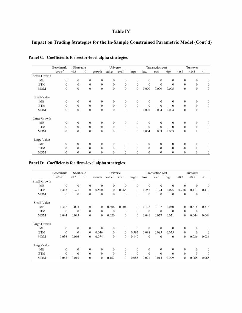
Table IV

Impact on Trading Strategies for the In-Sample Constrained Parametric Model (Cont’d) Panel C: Coefficients for sector-level alpha strategies

Panel D: Coefficients for firm-level alpha strategies

<0.5 0 growth value small large low med high <0.2 <0.5 <1Small-Growth

ME 0 0 0 0 0 0 0 0 0 0 0 0 0BTM 0 0 0 0 0 0 0 0 0 0 0 0 0MOM 0 0 0 0 0 0 0 0.009 0.009 0.005 0 0 0

Small-ValueME 0 0 0 0 0 0 0 0 0 0 0 0 0

BTM 0 0 0 0 0 0 0 0 0 0 0 0 0MOM 0 0 0 0 0 0 0 0.001 0.004 0.004 0 0 0

Large-GrowthME 0 0 0 0 0 0 0 0 0 0 0 0 0

BTM 0 0 0 0 0 0 0 0 0 0 0 0 0MOM 0 0 0 0 0 0 0 0.004 0.003 0.003 0 0 0

Large-ValueME 0 0 0 0 0 0 0 0 0 0 0 0 0

BTM 0 0 0 0 0 0 0 0 0 0 0 0 0MOM 0 0 0 0 0 0 0 0 0 0 0 0 0

Benchmark w/o rf

Short-sale Universe Transaction cost Turnover

<0.5 0 growth value small large low med high <0.2 <0.5 <1Small-Growth

ME 0 0 0 0 0 0 0 0 0 0 0 0 0BTM 0.413 0.371 0 0.500 0 0.268 0 0.252 0.174 0.095 0.278 0.413 0.413MOM 0 0 0 0 0 0 0 0 0 0 0 0 0

Small-ValueME 0.318 0.003 0 0 0.306 0.004 0 0.178 0.107 0.030 0 0.318 0.318

BTM 0 0 0 0 0 0 0 0 0 0 0 0 0MOM 0.044 0.045 0 0 0.020 0 0 0.041 0.027 0.021 0 0.044 0.044

Large-GrowthME 0 0 0 0 0 0 0 0 0 0 0 0 0

BTM 0 0 0 0.046 0 0 0.397 0.098 0.085 0.055 0 0 0MOM 0.036 0.066 0 0.074 0 0 0.140 0 0 0 0 0.036 0.036

Large-ValueME 0 0 0 0 0 0 0 0 0 0 0 0 0

BTM 0 0 0 0 0 0 0 0 0 0 0 0 0MOM 0.065 0.015 0 0 0.167 0 0.085 0.021 0.014 0.009 0 0.065 0.065

Benchmark w/o rf

Short-sale Universe Transaction cost Turnover

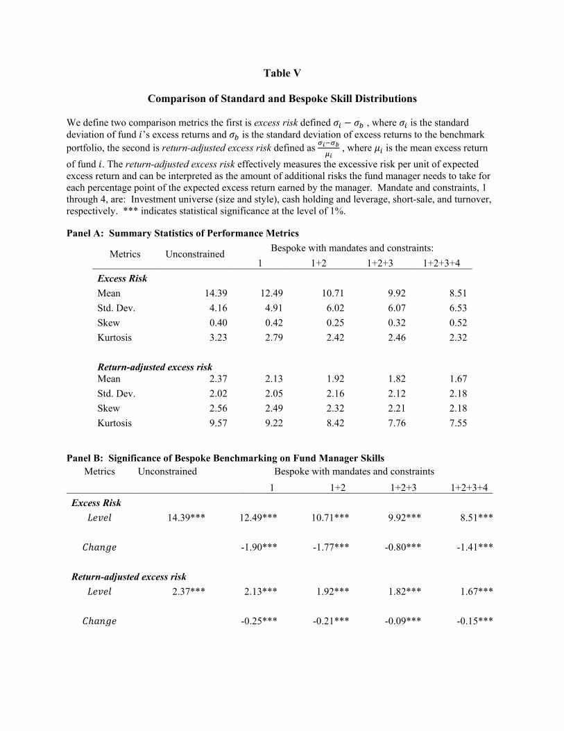
Table V

Comparison of Standard and Bespoke Skill Distributions We define two comparison metrics the first is excess risk defined 𝜎𝜎𝑖𝑖 − 𝜎𝜎𝑏𝑏 , where 𝜎𝜎𝑖𝑖 is the standard deviation of fund 𝑖𝑖’s excess returns and 𝜎𝜎𝑏𝑏 is the standard deviation of excess returns to the benchmark portfolio, the second is return-adjusted excess risk defined as 𝜎𝜎𝑖𝑖−𝜎𝜎𝑏𝑏

𝜇𝜇𝑖𝑖 , where 𝜇𝜇𝑖𝑖 is the mean excess return

of fund 𝑖𝑖. The return-adjusted excess risk effectively measures the excessive risk per unit of expected excess return and can be interpreted as the amount of additional risks the fund manager needs to take for each percentage point of the expected excess return earned by the manager. Mandate and constraints, 1 through 4, are: Investment universe (size and style), cash holding and leverage, short-sale, and turnover, respectively. *** indicates statistical significance at the level of 1%. Panel A: Summary Statistics of Performance Metrics

Metrics Unconstrained Bespoke with mandates and constraints: 1 1+2 1+2+3 1+2+3+4

Excess Risk Mean 14.39 12.49 10.71 9.92 8.51 Std. Dev. 4.16 4.91 6.02 6.07 6.53 Skew 0.40 0.42 0.25 0.32 0.52 Kurtosis 3.23 2.79 2.42 2.46 2.32 Return-adjusted excess risk Mean 2.37 2.13 1.92 1.82 1.67 Std. Dev. 2.02 2.05 2.16 2.12 2.18 Skew 2.56 2.49 2.32 2.21 2.18 Kurtosis 9.57 9.22 8.42 7.76 7.55

Panel B: Significance of Bespoke Benchmarking on Fund Manager Skills

Metrics Unconstrained Bespoke with mandates and constraints 1 1+2 1+2+3 1+2+3+4 Excess Risk

𝐿𝐿𝐿𝐿𝐿𝐿𝐿𝐿𝐿𝐿 14.39*** 12.49*** 10.71*** 9.92*** 8.51***

𝐶𝐶ℎ𝑎𝑎𝑎𝑎𝑎𝑎𝐿𝐿 -1.90*** -1.77*** -0.80*** -1.41***

Return-adjusted excess risk 𝐿𝐿𝐿𝐿𝐿𝐿𝐿𝐿𝐿𝐿 2.37*** 2.13*** 1.92*** 1.82*** 1.67***

𝐶𝐶ℎ𝑎𝑎𝑎𝑎𝑎𝑎𝐿𝐿 -0.25*** -0.21*** -0.09*** -0.15***

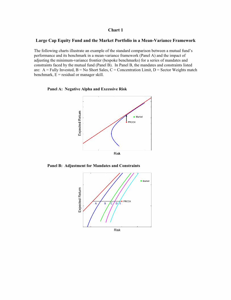
Chart 1 Large Cap Equity Fund and the Market Portfolio in a Mean-Variance Framework

The following charts illustrate an example of the standard comparison between a mutual fund’s performance and its benchmark in a mean-variance framework (Panel A) and the impact of adjusting the minimum-variance frontier (bespoke benchmarks) for a series of mandates and constraints faced by the mutual fund (Panel B). In Panel B, the mandates and constraints listed are: A = Fully Invested, B = No Short Sales, C = Concentration Limit, D = Sector Weights match benchmark, E = residual or manager skill.

Panel A: Negative Alpha and Excessive Risk

Panel B: Adjustment for Mandates and Constraints

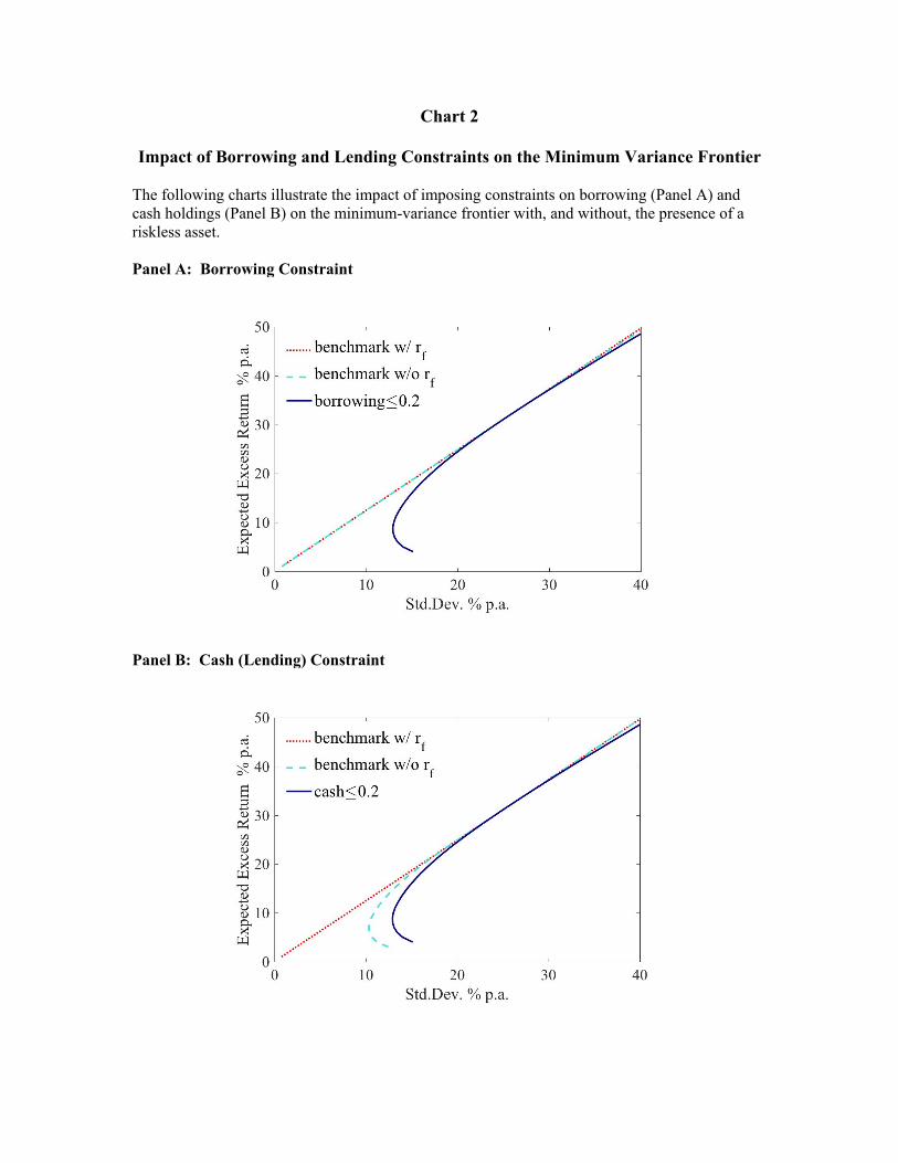
Chart 2 Impact of Borrowing and Lending Constraints on the Minimum Variance Frontier

The following charts illustrate the impact of imposing constraints on borrowing (Panel A) and cash holdings (Panel B) on the minimum-variance frontier with, and without, the presence of a riskless asset. Panel A: Borrowing Constraint

Panel B: Cash (Lending) Constraint

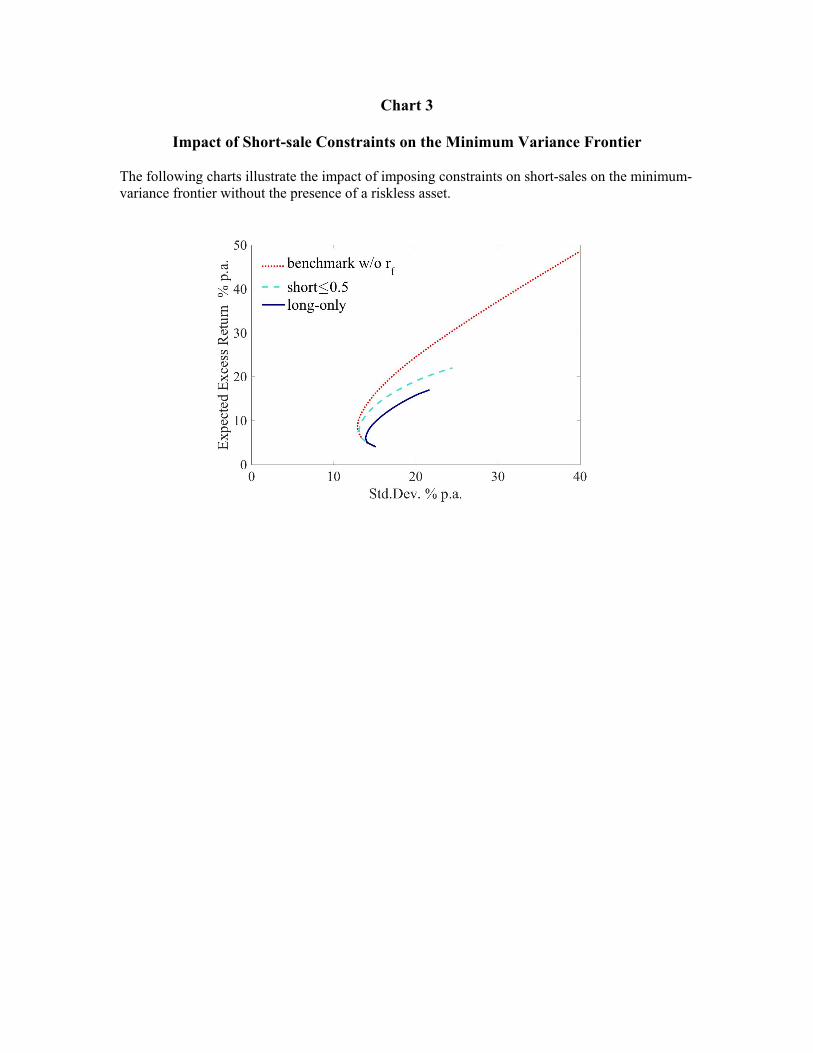
Chart 3

Impact of Short-sale Constraints on the Minimum Variance Frontier The following charts illustrate the impact of imposing constraints on short-sales on the minimum-variance frontier without the presence of a riskless asset.

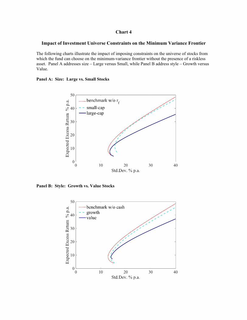
Chart 4

Impact of Investment Universe Constraints on the Minimum Variance Frontier The following charts illustrate the impact of imposing constraints on the universe of stocks from which the fund can choose on the minimum-variance frontier without the presence of a riskless asset. Panel A addresses size – Large versus Small, while Panel B address style – Growth versus Value. Panel A: Size: Large vs. Small Stocks

Panel B: Style: Growth vs. Value Stocks

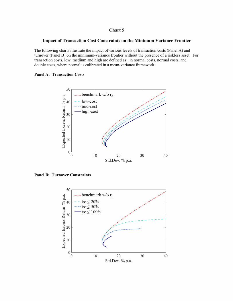
Chart 5

Impact of Transaction Cost Constraints on the Minimum Variance Frontier The following charts illustrate the impact of various levels of transaction costs (Panel A) and turnover (Panel B) on the minimum-variance frontier without the presence of a riskless asset. For transaction costs, low, medium and high are defined as: ½ normal costs, normal costs, and double costs, where normal is calibrated in a mean-variance framework. Panel A: Transaction Costs

Panel B: Turnover Constraints

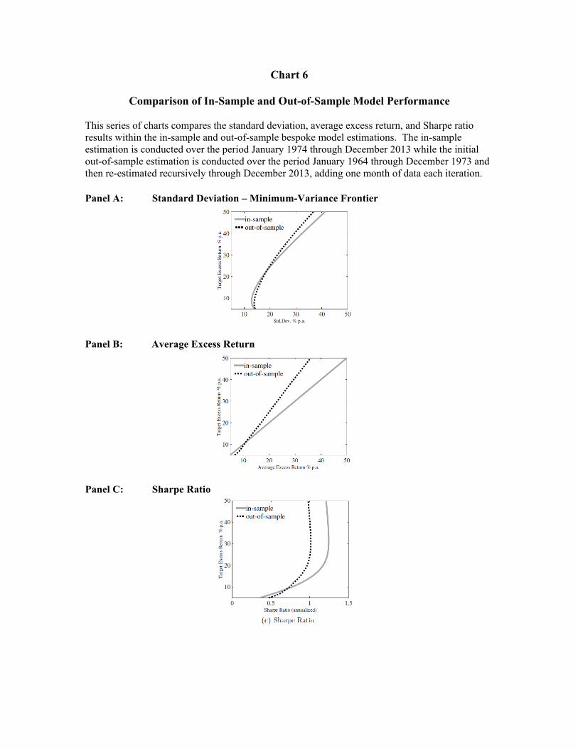
Chart 6

Comparison of In-Sample and Out-of-Sample Model Performance This series of charts compares the standard deviation, average excess return, and Sharpe ratio results within the in-sample and out-of-sample bespoke model estimations. The in-sample estimation is conducted over the period January 1974 through December 2013 while the initial out-of-sample estimation is conducted over the period January 1964 through December 1973 and then re-estimated recursively through December 2013, adding one month of data each iteration. Panel A: Standard Deviation – Minimum-Variance Frontier

Panel B: Average Excess Return

Panel C: Sharpe Ratio

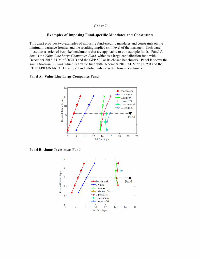
Chart 7

Examples of Imposing Fund-specific Mandates and Constraints This chart provides two examples of imposing fund-specific mandates and constraints on the minimum-variance frontier and the resulting implied skill level of the manager. Each panel illustrates a series of bespoke benchmarks that are applicable to our example funds. Panel A details the Value Line Large Companies Fund, which is a large-capitalization fund with December 2013 AUM of $0.21B and the S&P 500 as its chosen benchmark. Panel B shows the Janus Investment Fund, which is a value fund with December 2013 AUM of $1.75B and the FTSE EPRA/NAREIT Developed and Global indices as its chosen benchmark. Panel A: Value Line Large Companies Fund

Panel B: Janus Investment Fund

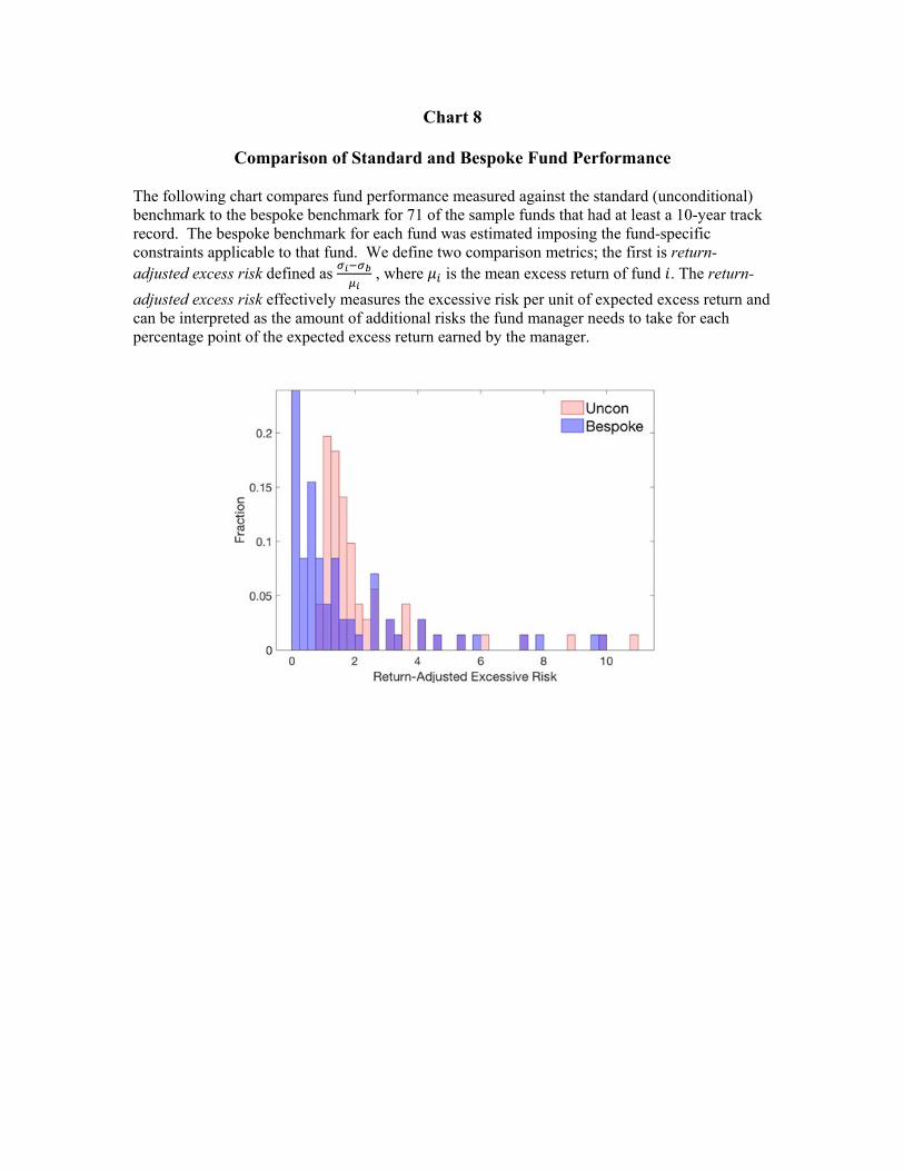
Chart 8

Comparison of Standard and Bespoke Fund Performance The following chart compares fund performance measured against the standard (unconditional) benchmark to the bespoke benchmark for 71 of the sample funds that had at least a 10-year track record. The bespoke benchmark for each fund was estimated imposing the fund-specific constraints applicable to that fund. We define two comparison metrics; the first is return-adjusted excess risk defined as 𝜎𝜎𝑖𝑖−𝜎𝜎𝑏𝑏

𝜇𝜇𝑖𝑖 , where 𝜇𝜇𝑖𝑖 is the mean excess return of fund 𝑖𝑖. The return-

adjusted excess risk effectively measures the excessive risk per unit of expected excess return and can be interpreted as the amount of additional risks the fund manager needs to take for each percentage point of the expected excess return earned by the manager.

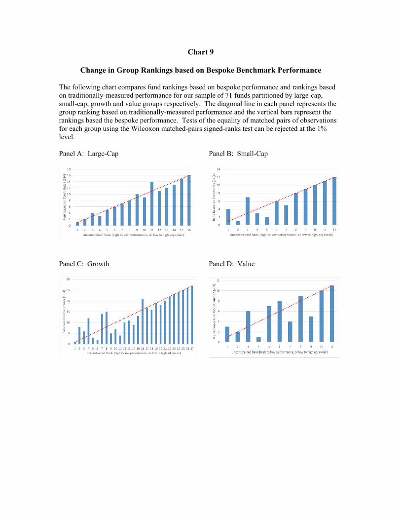
Chart 9

Change in Group Rankings based on Bespoke Benchmark Performance The following chart compares fund rankings based on bespoke performance and rankings based on traditionally-measured performance for our sample of 71 funds partitioned by large-cap, small-cap, growth and value groups respectively. The diagonal line in each panel represents the group ranking based on traditionally-measured performance and the vertical bars represent the rankings based the bespoke performance. Tests of the equality of matched pairs of observations for each group using the Wilcoxon matched-pairs signed-ranks test can be rejected at the 1% level. Panel A: Large-Cap Panel B: Small-Cap

Panel C: Growth Panel D: Value