Embed Size (px)
Citation preview

ASSESSING THE IMPACT OF REMITTANCES:
A CASE STUDY OF THE PHILIPPINES
by
Mustafa Zia
A thesis submitted to the Faculty of the University of Delaware in partial fulfillmentof the requirements for the degree of Master of Science in Economics
Spring 2011
Copyright 2011 Mustafa ZiaAll Rights Reserved

ASSESSING THE IMPACT OF REMITTANCES:
A CASE STUDY OF THE PHILIPPINES
by
Mustafa Zia
Approved: __________________________________________________________Peter Schnabl, Ph.D.Professor in charge of thesis on behalf of the Advisory Committee
Approved: __________________________________________________________Saul Hoffman, Ph.D.Chair of the Department of Economics
Approved: __________________________________________________________Rick L. Andrews, Ph.D.Interim Dean, Lerner College of Business & Economics
Approved: __________________________________________________________Charles G. Riordan, Ph.D.Vice Provost for Graduate and Professional Education

iii
ACKNOWLEDGMENTS
Falaris, Evangelos, Laurence Seidman for all of their advice and guidance.
Peter Schnabl, my advisor who was there to help me on a daily basis. Without hisimmense help this paper would not have been possible.
My mother, Hajera Zia, for her love and support.
iv
TABLE OF CONTENTS
LIST OF TABLES ........................................................................................................ viABSTRACT ............................................................................................................... ix
Chapter
1 INTRODUCTION.............................................................................................. 1
1.1 The Philippines Background .................................................................. 51.2 When did it Begin?................................................................................. 51.3 Who Are The Overseas Filipinos? ......................................................... 71.4 Characteristics of Overseas Filipinos: (The Latest year 2008) .............. 9
2 LITERATURE REVIEW................................................................................. 11
2.1 Remittances and GDP Growth ............................................................. 112.2 Remittances and Human Capital .......................................................... 132.3 Remittances and Health........................................................................ 172.4 Remittances and Inequality .................................................................. 192.5 The Multiplier Effect............................................................................ 22
3 THE DATA ...................................................................................................... 25
3.1 The Variables ....................................................................................... 28
4 METHODOLOGY........................................................................................... 33
4.1 Models 1-A & 1-B................................................................................ 344.2 Models 2-A & 2-B................................................................................ 364.3 Our Expectations from the Equations .................................................. 384.4 Inequality Analysis............................................................................... 40
5 RESULTS......................................................................................................... 42
5.1 Model 1-A & 1-B. ................................................................................ 425.2 Model 2-A & 2-B. ................................................................................ 435.3 Yearly Models 1, 2, 3, & 4 ................................................................... 45

v
5.4 Expenditure Results.............................................................................. 475.5 Inequality Analysis:.............................................................................. 49
6 SUMMARY & CONCLUSION ...................................................................... 51REFERENCES............................................................................................................. 54
AppendixA MODEL 1-A (REGIONAL) ............................................................................ 57B MODEL 1-B (PROVINCIAL)......................................................................... 60C MODEL 2-A (REGIONAL) ............................................................................ 63D MODEL 2-B (PROVINCIAL)......................................................................... 66E 1999 (REGIONAL).......................................................................................... 69F 2004 (REGIONAL).......................................................................................... 72G 2007 (REGIONAL).......................................................................................... 75H 2008 (REGIONAL).......................................................................................... 78I MODEL 3-A(REGIONAL/PROVINCIAL) .................................................... 81J MODEL 4-A (REGIONAL/PROVINCIAL) ................................................... 82
vi
LIST OF TABLES
Table 3.1 Table of Variables ................................................................................ 29
Table A.1 Effects of Remittances on Fraction of Years Completed:For Ages 7-1213-1819-247-24 ..................................... 57
Table A.2 Controlling For Non-Remittance Income Effects of Remittanceson Fraction of Years Completed:For Ages 7-1213-1819-247-24 .................................... 58
Table A.3 Effect of Remittances on Education & Medical Expenditures ............ 58
Table A.4 Controlling For Non-Remittance Income Effect of Remittanceson Education & Medical Expenditures ................................................ 59
Table B.1 Effects of Remittances on Fraction of Years Completed:For Ages 7-1213-1819-247-24 ..................................... 60
Table B.2 Controlling For Non-Remittance Income Effects of Remittances onFraction of Years Completed:For Ages 7-1213-1819-247-24 ..................................... 61
Table B.3 Effect of Remittances on Education & Medical Expenditures ............ 61
Table B.4 Controlling For Non-Remittance Income Effect of Remittanceson Education & Medical Expenditures ................................................ 62
Table C.1 Effects of Remittances on Fraction of Years Completed:For Ages 7-1213-1819-247-24 ..................................... 63
Table C.2 Controlling For Non-Remittance Income Effects of Remittanceson Fraction of Years Completed:For Ages 7-1213-1819-247-24 ..................................... 64
Table C.3 Effect of Remittances on Education & Medical Expenditures ............ 64
Table C.4 Controlling For Non-Remittance Income Effect of Remittances onEducation & Medical Expenditures ..................................................... 65
vii
Table D.1 Effects of Remittances on Fraction of Years Completed: For Ages7-1213-1819-247-24 ..................................................... 66
Table D.2 Controlling For Non-Remittance Income Effects of Remittanceson Fraction of Years Completed: For Ages 7-1213-1819-247-24 ..................................................................................... 67
Table D.3 Effect of Remittances on Education & Medical Expenditures ............ 67
Table D.4 Controlling For Non-Remittance Income Effect of Remittances onEducation & Medical Expenditures ..................................................... 68
Table E.1 Effects of Remittances on Fraction of Years Completed: For Ages7-1213-1819-247-24 ..................................................... 69
Table E.2 Controlling For Non-Remittance Income Effects of Remittances onFraction of Years Completed: For Ages 7-1213-1819-247-24 ..................................................................................... 70
Table E.3 Effect of Remittances on Education & Medical Expenditures ............ 70
Table E.4 Controlling For Non-Remittance IncomeEffect of Remittances onEducation & Medical Expenditures ..................................................... 71
Table F.1 Effects of Remittances on Fraction of Years Completed: For Ages7-1213-1819-247-24 ..................................................... 72
Table F.2 Controlling For Non-Remittance Income Effects of Remittanceson Fraction of Years Completed:For Ages 7-1213-1819-247-24 ..................................... 73
Table F.3 Effect of Remittances on Education & Medical Expenditures ............ 73
Table F.4 Controlling For Non-Remittance Income Effect of Remittances onEducation & Medical Expenditures ..................................................... 74
Table G.1 Effects of Remittances on Fraction of Years Completed: For Ages7-1213-1819-247-24 ..................................................... 75
Table G.2 Controlling For Non-Remittance Income Effects of Remittances onFraction of Years Completed: For Ages 7-1213-1819-247-24 ..................................................................................... 76

viii
Table G.3 Effect of Remittances on Education & Medical Expenditures ............ 76
Table G.4 Controlling For Non-Remittance IncomeEffect of Remittances onEducation & Medical Expenditures ..................................................... 77
Table H.1 Effects of Remittances on Fraction of Years Completed:For Ages 7-1213-1819-247-24 ..................................... 78
Table H.2 Controlling For Non-Remittance Income Effects of Remittances onFraction of Years Completed:For Ages 7-1213-1819-247-24 ..................................... 79
Table H.3 Effect of Remittances on Education & Medical Expenditures ............ 79
Table H.4 Controlling For Non-Remittance Income Effect of Remittances onEducation & Medical Expenditures ..................................................... 80
Table I.1 Regional Effects of Remittances on Different Percentile Ratios ......... 81
Table I.2 Provincial Effects of Remittances on Different Percentile Ratios ....... 81
Table J.1 Inequality Analysis: Gini Decomposition (Regional) Total IncomeVariable: TOTINC ............................................................................... 82
Table J.2 Inequality Analysis: Gini Decomposition (Provincial) Total IncomeVariable: TOTINC ............................................................................... 82

ix
ABSTRACT
In recent years, there has been a plethora of literature written on
remittances. While disagreements exist on the exact impact of remittances,
nevertheless, the overwhelming view paints that of a positive picture. According to the
World Bank, the amount of remittance received for 2010 amount to $325 billion. This
is particularly the case in middle and low income countries. In this paper, I examine
the impact of remittances on education, health, and inequality using the Annual
Poverty Indicator Survey from the Philippines. This paper uses the Philippines as the
country of choice since ten percent of its GDP is comprised of remittances. The
analysis is done using regional/provincial fixed-effects, Gini decomposition, and ratios
of different expenditure per capita percentiles. The results indicate a positive impact of
remittances on education and health. However, the effect of remittances on inequality
is not conclusive, and suggests additional research.

1
Chapter 1
INTRODUCTION
A friend of mine once told me — had it not been for the financial help
from his brother abroad, his family would not have been able to survive financially.
Like many others looking for a better opportunity, his brother was able to find his way
into Europe. In a month’s time, he was able to find a job and send money back home.
The remittances sent by him went a long way in improving and meeting the financial
needs of his family. My friend stopped working as a street vendor, and started going
back to school. A similar pattern followed with the rest of his siblings, all of whom
were working to support the family. In a couple of years, the family had gone from
struggling to meet daily needs to a financially stability. This isn’t an isolated case. In
fact, there are many individuals living in developing as well as underdeveloped
countries who rely heavily on overseas remittances as a source of income. According
to recent estimates by the World Bank, the amount of remittances received for the year
2010 amount to $325 billion, an increase of 6 percent from the previous year. And the
amount of people living outside of their country of birth is estimated to be around 215
million individuals, accounting for 3 percentage of the world’s population (a majority
of them from the developing nations). The overwhelming consensus among
academics, researchers, and general public is that remittances provide a boost to the

2
economy (especially if the economy is that of a developing country) (e.g. Ang 2007,
Taylor 1995, 2003, Yang 2008, etc). One positive aspect of remittances is that it can
provide countries with access to funds without them having to go into debt. Many of
the organizations that provide money for developing countries often require the
receiving country to direct the funds towards achieving goals that the providing
organization sees as appropriate. The World Bank often has certain priorities and
requirements as to where the funds given must be spent. Not following the goal of the
desired organization can have negative consequences for the fund-receiving country.
Among many, one obvious consequence is the denial of current and future funds for
the country. Remittances on the other hand provide countries with an indirect form of
assistance through their citizens. It is not surprising then, that many of the developing
countries include remittances as a big portion of their GDP. The Philippines is a
leading example, with remittances accounting for 10 percent of its GDP. Even at a
micro level, remittances received by households enable them to spend the money at
their own discretion—unlike other forms of financial aid. In this way, remittances
allow for freeing up of some of the money for the households. The households can
now meet their basic needs easily, leaving extra money to be spent on education,
healthcare and other areas. Some have argued remittances to be a form of safety net.
During economic crisis, remittances tend to stay stable, and thus provide a much
needed help during economic downfalls (although the current crisis challenges this
theory). They also provide a transfer channel for skills and technology from abroad,
especially of those individuals living in highly developed countries such as the United
3
States and the Europe. An example of this transfer channel includes a Filipino IT
student in the United States who builds a computer learning school back home. The
list of positive impacts is quite exhaustive, but the point remains, remittances play a
vital role in the developing nations. Nevertheless, there are critics who seem to paint
a negative picture of the impact of remittances (e.g. Chami 2003, Haskar, Burges
2005, etc)
One criticism is that heavy reliance on remittances as a source of income
is problematic if there was a halt to the remittance sending and receiving system. A
halt could be due varying factors that either make it impossible or expensive to send
money back (e.g. high cost of transaction). This issue could be disastrous for a
country like the Philippines. For example, if a family relies heavily on assistance from
overseas for education expenses, then a sudden halt in that process could lead to the
discontinuation of educational attainment. If it persists, then this will obviously have
long-term negative direct and indirect external effects on the society (especially when
aggregated across households).
Another major criticism of remittances has been centered on the argument
that the money does not reach the neediest of individuals. Critics argue that only the
well off individuals have the ability to go abroad, and therefore those who benefit
most from these remittances aren’t the really needy ones. Additionally, the banking
system in developing nations makes it very hard for poor people to have an account,
which leads the poor to choose other alternatives. This could not only result in costs
for the poor in terms of transfer of the money, but also leads to the remittances not

4
being accounted for in the overall economy—creating an underground economy in the
process.
While there seem to be two opposing views of remittances on many socio-
economic factors, in this paper I will examine the effects that remittances have on
education, healthcare, and inequality. The reason for using the Philippines as a country
of interest is because the Philippines is famous for its export of workers. According to
the World Bank, the Philippines is the fourth largest recipient of remittances.
Moreover, in 2010, the Philippines received $21.3 billion dollars in remittances, right
behind Mexico ($22.6 billion), China ($51 billion), and the top remittances receiving
country, India ($55 billion). This paper is divided into six main sections. The first
section deals with some background information on the Philippines, its migration
pattern, and the characteristics of the Filipino migrants. The second section discusses
some of the literature related to the impact of remittances on various facets of the
economy. In the third section, more attention is given to the data sets relevant for this
paper. This part discusses some of the data sets specifications, as well as the variables
relevant for this paper. The next two sections, four and five, deal with methodology,
and the results found in this paper. That is, the fourth section discusses some
specifications of the fixed-effects regressions, the decomposition of total income, and
different expenditures per capita ratios to examine inequality. Section five pertains to
the results attained after running the regressions. I will discuss about the significance
as well as the magnitude of some of the coefficient estimates achieved. The last

5
section concludes the paper with a review of the results and some recommendations
for future analysis.
1.1 The Philippines Background
Located in the Western Pacific Ocean of Southeast Asia, the Philippines is
considered one of the biggest exporters of labor. The Philippines is estimated to have
the highest rates of outmigration to population compared to any other countries in East
or South East Asia (Lucas, 2001). The remittances are quite pronounced—currently
constituting 10% of the entire Philippines GDP. According to the Commission on
Filipinos Overseas, in 2009 there were 8.6 million Filipinos overseas. Of this 8.6
million, 4.1 million of them were permanent migrants, 3.9 million of them were
temporary migrants, and there were more than 6 hundred thousand irregular migrants.
It is vital to look at the history of when migration became important for the
Philippines.
1.2 When did it Begin?
In 1974 the government of the Philippines instituted international
migration as policy to combat the temporary problem of unemployment. The
Presidential Decree number 442 (a Labor Code of the Philippines) was the reason
behind the creation of the Overseas Employment Development Board. A department
created to foster Filipino employment overseas, as well as to register and monitor
Filipinos overseas. However, since its inception, there has been a concerted effort to

6
facilitate the export of labor overseas, not merely on temporary basis, but as a long-
term revenue generator for the Philippine economy. Due to an increase in the number
of Filipinos migrating to other countries, the President had to create an independent
department—solely responsible for dealing with Filipinos leaving overseas. To that
effect, in 1978, the President ordered the creation of the Office of Emigrant Affairs
(Decree number 1412). This wasn’t to be the last expansion of the office, as the
outflow of Filipino migrants grew.
The high volume of migrants resulted in the formation of Batas Pambansa
Blg. 79 (established on June 16th of 1980)—which replaced the Office of Emigrant
Affairs (OEA). The latter expanded its functions to include the welfare and interest of
migrants leaving the Philippines. The four main functions of Batas Pambansa Blg. 79
are as follows:
“Provide assistance to the President and the Congress of the Philippines
in the formulation of policies and measures concerning or affecting
Filipinos overseas;
Develop and implement programs to promote the interest and well-
being of Filipinos overseas;
Serve as a forum for preserving and enhancing the social, economic,
and cultural ties of Filipinos overseas with the motherland; and
7
Provide liaison services to Filipinos overseas with appropriate
government and private agencies in the transaction of business
and similar ventures in the Philippines” (Overseas Filipinos
Website).
The gradual transformation of the offices dealing with overseas migrants
is an indicator of the vital role that overseas Filipinos play in the local Philippines
economy. Going from a policy that didn’t “promote overseas employment as a means
to sustain economic growth and economic development (Section 2c, Republic Act
8042)”, to considering the employment of overseas Filipinos as a “legitimate option
for the countries work force”—forcing the government to “fully respect labor
mobility, including the preference for overseas employment.”(Go Undated). In
addition to the history of labor migration, it is also important to know a little about the
overseas Filipino migrants.
1.3 Who Are The Overseas Filipinos?
Filipinos living overseas can be divided into three groups. The groups are
classified as permanent migrants, temporary or non-migrants, and lastly irregular
migrants.
-Permanent Migrants: These are the migrants who have left the
Philippines on the premise that they will reside abroad, and have no intention of

8
coming back to live in the Philippines. As indicated earlier, these migrants constitute
the largest bulk of the overall Filipinos abroad (4.1 million out of the 8.6 million).
-Temporary or non-migrant: These are migrants who have left the country
primarily to work, and have the intention of coming back once their work contract is
over. The duration of time for temporary migrants is usually more than 6 months. This
group constitutes the second largest bulk of Filipino migrants, amounting to 3.9
million of the total migrants abroad.
-Irregular migrants: The smallest portion of Filipinos living abroad is
those who have left the Philippines with or without any proper authorization, or
documentation, but due to legal issues lost their status abroad. These immigrants may
have lost their status due to legal issues or because they have overstayed their time in
the foreign country (Asis.). There is also a difference in terms of where most Filipinos
are attracted to migrate.
The top destination countries as of 2010 are United States, Saudi Arabia,
Canada, Malaysia, Japan, Australia, Italy, Qatar, the United Arab Emirates, and the
United Kingdom. However, the top region in terms of Filipino migration has
consistently been the Middle East. There is however a distinction between the top
destination, and the top source countries. The top source countries provide the largest
percentage of remittances as a source of income for the Philippines. As expected, the
top source country is the United States, followed by China, United Kingdom, Bahrain,
Japan, Antigua and Barbuda, Indonesia, India, Brazil, and Angola. It should also be
noted that since the 1970s the pattern and trend of Filipino workers have changed. For

9
example, during the 1970s many of the overseas Filipinos were unskilled workers,
who mainly went to the Middle East. However, as the decades went by, the demand
for high skilled and in particular service industry has increased substantially. The
United States, and many other developed countries are in high demand for service
industries such as Nursing and Information Technology. Thus, we have seen an ever-
increasing number of Filipinos specializing in medical and information technology
fields. It is also important to point out that the male to female disparity of migrants
has also diminished as the demand for more service oriented jobs increased. Many of
the Nursing jobs are particularly suited towards women, and thus we have seen an
increasing drop in the male to female ratio of workers and immigrants abroad. It is
also vital to mention some information on the characteristics of these overseas
Filipinos.
1.4 Characteristics of Overseas Filipinos: (The Latest year 2008)
This section, based on the Overseas Filipinos Survey conducted by the
National Statistics Office provides data on the Filipinos living abroad. It includes
individuals who are 15 years and older, have left the country within the last five years,
and are working or had worked abroad during the past six months. According to the
survey, there were an estimated 2 million Overseas Filipinos Workers (OFWs) who
worked abroad. The portion of male compared to female workers was slightly higher
(51.7% male to 48.3% female), and more than ¼ of the workers were between the ages
of 25 and 29 (25.7%). The ages of male workers seemed to be smoother in terms of

10
distribution, as compared to females. Of the total number of female workers abroad,
28.8 percent belonged to the age group 25-29, and 20.3 percent belonged to the age
group 30-34.
About one third (34.7percent) of the total of OFWs belonged to the
laborers and unskilled workers group. This group included workers in cleaning,
manufacturing, and domestic helping. 15 percent of the workers belonged to the trade
and other trade related workers, while service workers and shop market sales workers
constituted 14.3 percent of the total number of workers. Finally, plant and machine
operators and assemblers made up the last big bulk of the OFWs.
The top five regions that constituted most of the OFWs are
CALABARZON (14.7 percent), National Capital Region (12.8 percent), Central
Luzon (11.8 percent), Llocos Region (8.3 percent), and finally Cagayan Valle (7.3
percent). These five regions amount to about 50 percent of the Filipinos workers
overseas. The next section sheds some light on the literature related to remittances. In
particular, the literature relating remittances to education, health, inequality, and the
multiplier effect of remittances. (National Statistics Office)
11
Chapter 2
LITERATURE REVIEW
Remittances have several impacts on the economy. This paper will only
showcase some of the most important linkages between remittances and factors that
are paramount to a developing nation. In this section I will converse some of the
literature written about the impact of remittances on various economic factors. I will
try to mention both sides of the argument; that is literature that does not have a
favorable view of remittances, and literature that shows deems remittance impact
positive. One of the most important areas in which remittances may play an important
role is the overall GDP of a country. Remittance growth has long been related with
GDP growth.
2.1 Remittances and GDP Growth
Several countries such as Bulgaria, Philippines, Pakistan, India to name a
few, consider remittances to be a vital part of their overall economy. There has been a
plethora of literature written on this subject matter, with most of the academic
consensus being that remittances have a positive impact on GDP. Nevertheless, there
are those who negate the view that remittances have a positive impact on GDP.
Several authors such as Chami et al (2003), Burgess and Haksar (2005) have found a
negative correlation between remittances and economic growth. Burgess and Haksar

12
find that the growth rate of remittances is inversely correlated with the per capita GDP
growth, using data from the mid-1980s. They use Ordinary Least Squares (OLS) as
well as Instrument Variable (IV) methods to come up with their conclusion. Using
OLS, they regress the log of real GDP per capita on the investment to the GDP ratio,
and the log of worker remittances to GDP. In their OLS analysis they find a negative
correlation between per capita GDP and the growth rate of remittances. However, due
to the possibility of an endogeniety problem (between per capita growth in real income
and remittances) they conduct an Instrument Variable regression. Using the IV
method, their regressions yield inconclusive results. They attribute their coefficient
estimates for both methods to data problems (in particular the 1998 dataset). When
the authors include the 1998 data set, they get a negative correlation compared to
when they do not include the 1998 observation for remittances. Therefore, they do not
find empirical evidence to support that remittances have a positive effect on the GDP.
Burgess and Haskar base most of their study on Chami’s paper. Chami also found a
negative relation between GDP and remittances.
In his paper, Chami creates a unified model to examine the outcome of
remittances on the economy. He finds remittances to have negative impact on real
growth in per capita incomes, due to the problem of adverse incentive. That is, since
the whole remittance process takes place in an uncertain economic environment, it
leads to a reduction of economic activity. However, his findings are most likely
convoluted as he aggregates cross-country data to make a unified model. This is a
problem, since each country has distinct characteristics. Therefore, the effects of

13
remittances on GDP growth will also depend on country specific characteristics (i.e.
political stability, level of corruption, etc). This is the case with a study done by Alvin
P. Ang. In his paper, “Workers’ Remittances and Economic Growth in the
Philippines”, Ang (2007) concludes that the relationship between GDP growth and
remittance growth is positive and statistically significant. Ang’s study is based on a
country per country analysis, while Burgess-Haskar and Chami use cross-sectional
analysis and a unified model respectively. That is a problem, since country
characteristics and factors affecting migration and remittances change over time and
do not tend to stay constant. Thus, the unified model suggested will not be able to
account for those factor changes and will yield inconclusive results. In that sense, a
country by country analysis is vital in order to clearly understand the impact of
remittances in GDP and overall development. Although Ang does acknowledge the
possibility of an endogeneity problem in the study, nevertheless, the results seem to
confirm the anecdotal evidence among many Filipinos—remittance growth does have
a positive effect in the GDP growth. GDP is one side of the coin—remittances affect
other socio-economic factors. This impact is very pronounced in the field of
education.
2.2 Remittances and Human Capital
Anecdotal evidence shows that remittances have long been seen as a
positive factor in education attainment. The list of scholars analyzing the various
relations between remittances and education is quite exhaustive. A few of them will

14
be mentioned in this paper. Among many scholars, Dean Yang is the one who has
written some important papers on this subject matter. Yang (2008) examines the role
that an exchange rate shock plays in remittances, which in turn affects various
household investments such as child schooling, child labor, and entrepreneurial
activity. He uses the exchange rate shocks as an instrument for remittances in his
Instrument Variable regression. The idea is that an exchange rate shock appreciates
the value of the currency, and thus the remittances sent back are worth more than they
were before the exchange rate changed. He estimates the Philippines-peso remittance
elasticity with respect to exchange rate to be around .60, which is quite large. He
rejects the notion that remittances are primarily consumed. Rather his results indicate
that remittances play an investment role in the Philippines, in particular on education.
Accordingly, families who were affected by the exchange rate shock were able to raise
their non-consumption investment (i.e. human capital investment). Moreover, those
families tended to keep their children longer in school, reduced the responsibility of
the child in terms of providing for the family (reduce child labor), and embark on
entrepreneurial activities (start capital-intensive enterprises).
In, “Accounting for Remittance and Migration Effects on Children’s
Schooling”, Dorantes and Pozo (2010) find mixed results. Using data from the
Dominican Republic, the authors study the effects of remittances on school
attendance. Dominican Republic is one of the countries that has experienced an
extensive amount of migration, in particular to the United States. According to the
15
2009 estimates of the World Bank, 12 percent of the population has already emigrated,
and remittances amount to approximately 10 percent of the country’s total GDP.
The study distinguishes between two kinds of households, those with a
member of the family who has migrated to the United States (migrant households),
and those who do not have a migrant member of the family in the United States (non-
migrant households). The authors opt to choose the non-migrant households to
conduct their analysis, because non-migrant households’ children constitute 88 percent
of their entire sample. Thus, non-migrant households become a more reliable sample
to utilize. However, the study claims that 52 percent of children who receive
remittances reside in non-migrant households. Their results suggest that remittances
do have a positive impact on the children’s school attendance. In addition to a 3
percent point increase in the likelihood of attending school (due to a 10 percent
increase in the likelihood of receiving remittances), girls’ attendance as well as the
secondary school age children and younger siblings seem to reap a large chunk of the
benefits from remittances in terms of school attendance. However, they get a different
result when they expand their datasets to include migrant households. In other words,
their study shows that the migration of a family member tends to have a negative and
disruptive effect on school attendance of children. For instance, male member of the
family (usually father) is the head of the household. Having a big influence in the
households, the absence of the father will surely have a negative impact on the family.
This is most certainly the case if the children in the household are young.
Nevertheless, the study does not see a negative impact of remittances, rather, a

16
disruptive effect on school attendance due to migration. Thus the study confirms the
general notion of a positive feedback from remittances on human capital investment.
There were also several other studies done, which examine other types of
correlations between remittances and education. Edwards and Ureta use El-Salvador to
study the effects of remittances on school retention— they find the relation to be
significant. In particular, they examine the effects on school retention rates from
different income sources. They find remittances to have a bigger impact on the school
retention rate, compared to other sources of income. The study was done using a Cox
proportional hazard model. (Edwards –Cox and Ureta 429-461)
Needless to say, there has been an overabundance of literature written on
the subject matter—all the same, the overwhelming majority paint a positive picture of
the effect of remittances on education attainment.
Aside from educational attainment, remittances sometimes provide a good
source of income to be expended on healthcare. The impact of remittances on
healthcare is difficult to explain. Remittances can have a consumption effect on
healthcare. For example, a family can ameliorate an immediate medical problem due
to remittances (e.g. going to the dentist). On the other hand, remittances might
provide a continuous stream of income that enables a family to improve its overall
health (e.g. seeing a dentist on a regular basis). This impact of remittances can then be
categorized as human capital investment effect. There have been attempts by some
scholars to shed light on this phenomenon.
17
2.3 Remittances and Health
Studying the effects of remittances on health expenditure in Mexico, Jorge
(2008) uses a Tobit model with fixed-effects. In particular, the author wants to see if
the share of household health expenditure in total expenditure is affected by
remittances. The study finds a significant link between the level of remittances and
health expenditure. For individuals in households who lacked medical care, and were
not covered by any other type of insurance, the effect of remittances on their level of
health expenditure was significant. This means that remittance do in fact increase non-
consumption activities. The authors found a 10 percent of changes in remittances to be
associated primarily with health expenditure. The results were also verified using both
a Tobit as well as a Generalized Least Squared (GLS) model. Both of the models
confirmed the theory, that remittances positively affect a household’s health
expenditure (Jorge). A similar effort to study the effects of remittances on health was
produced by Hildebrandt and McKenzie (2005).
Hildebrandt and McKenzie look at the effect of migration on child health
in Mexico. Using various econometric methodologies (OLS, IV, Probit), the authors
investigate this issue with the 1997 nationally representative demographic survey.
Overall the authors’ find a linear relation between migration and child health. In
particular, the authors note a decrease in the incidence of child mortality and increase
in higher birth weights—the two indicators used as proxies for health outcome.
Although the authors find the effects of migration to be larger than remittance, they
nevertheless contend that remittances do have positive impact on health outcomes.
18
Using a Grossman production function, they label remittances as a positive channel of
migration on health outcomes. Alternatively, migration influences health outcomes
through the wealth mechanism. That is, individuals who receive remittances are more
capable, and possibly likely to spend on health related activities. There is also a
possibility of remittances affecting health outcomes indirectly through consumption.
Although farfetched, it is possible for households to increase their overall food
consumption, which could result in better health. This will specially be the case if the
food purchased is of high nutrients such as vegetables and fruits. Again, the evidence
in the case of health outcomes seems to follow anecdotal evidence—that remittances
have positive effect on health (Hildebrandt, and McKenzie 257-289).
A different, yet theoretically similar approach was taken by Chauvet,
Gubert, and Somps (2008) to see if remittances are more effective than aid in
improving child health.
They measure it by looking at child and infant mortality rates, as well as
stunting incidence. The analysis examines the effects of aid, remittances, and medical
brain drain has on health outcomes. According to the authors, both aid as well as
remittances have a positive impact on health outcomes, albeit aid is more helpful for
the poor than remittances. Medical brain drain, which occurs when those individuals
in the medical field migrate to other countries, seems to have a negative impact on
health outcomes. Medical brain drain also results in aid becoming less effective, due to
a decrease in the number of qualified medical professionals who serve as a
compliment to aid. Nevertheless, in terms of remittances, the impact on health

19
outcomes seems to be positive, even if it is mainly for the children of the richer
portion population. This most likely exacerbates inequality, which is another
important factor that needs attention. (Chauvet, Gubert, and Somps)
2.4 Remittances and Inequality
There has been some argument to whether the remittances sent back
increases the income distribution gap. The premise is that most of the well-off
families are capable of migration, and thus remittances sent back only magnifies the
inequality gap. There have been several studies conducted to clarify this topic.
According Ang (2007), while remittance growth might lead to GDP growth,
remittances also seem to exacerbate the inequality issue. According to the study, most
of the OFWs comes from certain regions (Regions I, III, IV, VI, XI, and NCR), which
are regions that already have lower rates of poverty. This also goes to prove Taylor’s
(2006) point that most of the immigrants are not from poor families, and thus the
migration might actually exacerbate the poverty issue. Ang further emphasizes that
the regions with highest rates of migration are more urbanized compared to other
regions. A different approach to examine this issue is taken by Jones (1998).
This is a study done with the 1998 household survey of central Zacatecas
state, Mexico to find the effect of remittances on inequality. The study suggests that
previous studies of the effect of remittances on inequality have been inconclusive. He
offers a “spatiotemporal perspective” which uses migration stages and spatial scale
(interregional, interurban, rural-urban, and interfamilial). They are conceptualized as

20
controls which measure inequalities. With regards to the stage of migration, he finds
that the inequalities decrease with migration up to a point, after which it increases. At
the geographical scale, he finds the advantage going to the richer families, at the
expense of poorer families. Furthermore, he believes that at a regional and familial
level, remittances can play an important role if these regions are being introduced to
liberalized trade. While the richer regions might be affected by “foreign exchange-
generation activates”, it is only the poorest regions that seem to have a higher benefit
from remittances. Remittances seem to play a vital role in maintaining these regions,
which otherwise would have disappeared. The rural households are able to maintain
their “rural roots” while coping with the modern age. Moreover, the migrants seem to
invest more in non-consumption activities which makes them less likely to migrate.
Investments in human capital, health, and agriculture are some of the most important
ones made in these rural communities. Therefore, remittances according to Richard do
not exacerbate inequality, but rather provides an essential option for the poor in the
rural regions. The author provides a broader approach of looking at the inequality
issue than the existing literature. Another approach to looking at the impact of
remittances on inequality is conducted by Chimhowu, Piesse, and Pinder.
The Socioeconomic Impact of Remittances on Poverty Reduction is one of
the chapters of a book organized by the World Bank to have a comprehensive study of
remittances. The authors, Chimhowu, Piesse, and Pinder (2005), examine the
socioeconomic impact of remittances on poverty reduction. They conclude that
remittances have different effects based on different time horizons. First and
21
foremost, the authors believe that there needs to be a medium to long range horizon,
during which the full effect of remittances on poverty can be assessed. While in short
time, it is possible that it could increase a household’s consumption. However, the
long term implications are unclear. For example, a household might use the
remittances as a source of education or health expenditure, which can have a positive
future effect. Therefore, in the short-term remittances is very unlikely to lift a family
out of poverty, and medium to long term horizon is needed to fully count for the
effects of remittances on poverty. Nevertheless, the authors show that empirical
studies have shown that remittances “make a powerful contribution to reduction
poverty and vulnerability in most households and communities”.
Remittances might lead to inequality at a local level, but they might also
decrease it at an international level with the transfer of resources and knowledge from
developed to developing nations. On the national level, remittances could have a
negative impact if the country of interest has lower GDP and higher migration rate.
The studies indicate an increase in poverty for the families who do not have remitting
migrants, especially if a macroeconomic crisis is caused due to remittances inflows.
Although, according to the authors if a country has an organized system of migration
and remittances (such as the Philippines), then the impact of remittances is
significantly positive. In addition, they seem to have a negative outlook of what they
regard as “medical brain drain”, in which the individuals who have some sort of
degree in the healthcare field (nurses, physicians) will have a negative impact on the
overall healthcare system if these individuals decide to migrate. The idea is that while

22
the aid might be available to the country in focus, the lack of individuals who know
how to best utilize the aid will make the aid useless. Their results however are cross-
sectional, and there have been several studies which recommend focusing on a country
by country basis to have a solid analysis of the impact of remittances (e.g. Ang’s
analysis). Regardless of positive or negative impact, remittances seem to have a
multiplier effect on many socio-economic factors—and a mention of this effect is vital
in understanding the effects of remittances.
2.5 The Multiplier Effect
So far proponents of remittances seem to suggest that remittances have
multitude of effects in a country. Remittances given in a household might have
secondary or even tertiary effects on the entire economy. For example, remittances
sent back might result in the household investing more in education and healthcare.
This can have a big impact on children especially, since better health allows the
children to focus more on school. A multitude of literature has shown that more
schooling leads to higher income and lifestyle in the future.
In one study done by Glytsos (1993), the effects of international
remittances on production, imports, and employment on the Greek economy in 1971 is
examined. According to the author, the remittances have a multiplier effect of 1.71 on
GDP, with the biggest effect of remittances being on machinery and construction
industries. This means that a $2 million increase of remittances will lead to a $3.5
million increase in total GDP. Similar analysis has been done by other scholars.
23
Taylor has done several studies in which his analysis sheds some light on
the multiplier effects of remittances. In his 1995 analysis of international remittances
on a Mexican village, he finds a multiplier effect of 1.6. Similar to the Glytsos study,
a $2 million increase in remittances would lead to $3.2 million in the villages’ value
added output.
In 2003 Taylor conducted another study in which he examined the effects
of remittances on crop and household income. While the study found a negative effect
(lower crop yields and income) of migrants leaving the household, there was a positive
effect of remittances received by households. For example, the households tended to
substitute capital for labor as they were able to buy more inputs. Overall, the
remittances lead to an income increase of between 16 to 43 percent for members of the
rural households in China.
Finally, during the 2008 period, another study on Mexico was done by
Taylor and Dyer, in which they found a 52 percent increase in marginal human capital
investment and 5 percent increase in rural wages in the short run (due to an increase of
10 percent in remittances). The same was true for the long-term, except the effects
were even greater in terms of human capital investment. Overall the indirect effects of
remittances exceeded the direct effects of remittances. And this seems to confirm to
the notion that remittances do more than increasing household consumption. It affects
human capital and health investments which all have been proven to have positive
external effects.
24
Even though there have been some conflicting views on the effect of
remittances; the general notion seems to point towards a positive outcome. In recent
years, the United Nations has written several papers, and has spent considerable
resources in trying to understand fully, the effects of remittances. The United Nations
and many other international organizations, such as the International Monetary Fund
(IMF) all seem to think of remittances as having a positive effect on the developing
nations. It is to that effect, that many of the recent surveys run by the United Nations
include gather data on remittances. That is also the case in the Annual Poverty Report
survey of the Philippines. A survey conducted to measure several poverty indicating
variables. Abbreviated as APIS, this dataset was also used for this paper.

25
Chapter 3
THE DATA
The data collected for this paper are for four different years. The years in
interest are 1999, 2004, 2007, and 2008. The data used for this paper is cross-
sectional for each individual year, and it was originally collected by the National
Statistics Office in the Philippines. Although different sorts of survey were conducted
for each individual year, the survey from which the variables are taken is called
Annual Poverty Indicator Survey (for all four years), which is funded by the United
Nation and the Asian Europe Meeting (ASEM) organization.
The Annual Poverty Indicators Survey of 1999 was conducted using
40,922 households. Of the 40,992 sample households, 37,454 households were
successfully interviewed using the APIS. This means that the response rate was 91.4
percent successful. Those individuals who were not interviewed either refused to be
interviewed, or were not available during enumeration. It should be noted that the
sampling method used was similar to the one used for the 1995 Census of Population.
The purpose of the survey was to provide impact indicators that could be used as
inputs to monitor and analyze poverty indicators. Statistics on poverty for the
Philippines are presented in the Family and Income Expenditure Survey (FIES) which
was conducted on a three years basis since its introduction in 1995. Other than the

26
poverty indicators, the FIES also provides data on spending pattern by income class,
income deciles, etc. However, if there is no FIES survey conducted, then the National
Statistics Office of Philippines conducts the APIS. For this reason, the paper uses
APIS rather than FIES, since no FIES was conducted during the years of interest.
Additionally, FIES was not available from their databank. The sample also covered
82 provinces and 16 regions, including cities and municipalities. Included are also
3416 sample enumeration areas (EAs) or barangays with an approximately 41000
sample families. The weighting for the sample was conducted in three stages. The first
stage involves adjusting the weight at the stratum level (domain city, urban or rural,
within province). The adjusted factors were based on a division of sample EAs in the
stratum by the sample EAs actually enumerated. The second stage was adjusted for
non-interview households at the level of sample EA. Finally, in order to reflect the
change in population overtime, a weight adjustment factor based on population
projection was conducted. The adjustment factor was applied at the domain level, and
was based on best population projections for the survey year. The 2004 survey is more
or less similar to the 1999 survey.
Conducted in 2004, the survey has 48115 sample households, of which
42789 were successfully interview. The survey yielded a significant response rate of
88.9 percent at the national level. The sampling procedure for 2004 uses the Master
Sample from the 2003 year. The Master Sample utilizes a multi-stage sampling design
which involves three stages of evaluation. For example sample barangays are selected
with probability proportional to size in the first stage. Similar to the 1999 census, the

27
2004 census provides information not only on a country level, but at a regional level
as well (17 administrative regions included in this survey). A similar weighting
method as that of 1999 was used to ensure that the data is a good representative of the
whole country as well as its regions. The 2007 follows a similar pattern as the 1999,
and 2004 surveys.
The 2007 census has approximately 43107 household samples, of which
40239 were successfully interviewed (a response rate of 93.3 percent). Aside from not
being available or refusing to be interviewed, those who were in critical areas were
also excluded from this survey. Therefore, regions with political instability comprised
smaller percentage of the survey. This issue is prevalent throughout all the years in
this survey. That is, regions with political instability, such as the Autonomous Region
in Muslim Mindanao have lower response rates compared to the stable ones (e.g.
National Capital Region). In fact, the Autonomous Region in Muslim Mindanao is the
only region that has its own separate local government. The 2007 sample used the
2000 Census of Population and Housing survey as its master sample. The survey was
conducted in all of the 17 regional levels, and it was weighted similar to other years
(goes through three separate weighting stages) to ensure that the data is a good
representation of the country and its regions.
Following similar pattern as that of the previous 3 surveys, the 2008
APIS was conducted due to the absence of the Family Income and Expenditure Survey
(FIES). The APIS provide critical poverty statistics for the whole country as well as
the 17 different regions. Funded by the government of the Philippines, the survey

28
covered 43020 sample households of which 40613 households were successfully
interviewed. This translates to a response rate of 94.4 percent at the national level.
Although there is a visibly similar pattern among all the years of survey mentioned in
the paper, there are some notable variations that need mentioning. First of all, aside
from regional poverty statistics, the 1999 and 2004 APIS surveys include data on
provincial level analysis as well. This is not the case for the 2007 and 2008 APISs.
Secondly, there is no Region IV in the 2004, 2007, and 2008 surveys. Region IV was
split into two regions in 2002, resulting in Region IV-A (Calabarzon), and Region IV-
B (Mimaropa) which are included in the other years.
3.1 The Variables
There were a total of 17 variables selected from the different years. Some
variables were available for some years, but not for others (e.g. Visit to Health
Facility, Province). However, not all variables were used for this analysis, and
therefore the missing variables for certain years do not play a significant role in the
overall analysis. There was also a set of variables created by manipulating the
variables attained from the datasets. The following table provides the names and
description variables used and created for this paper:

29
Table 3.1 Table of Variables
Variables Description
Region
This variable shows the 17 different regions to which thehouseholds belong to. The 17 regions in no particular order are,llocos, Cagayan Valley, Central Luzon, Bicol, Western Visayas,Central Visayas, Eastern Visayas, Zamboanga Peninsula,NorthernMindanao, Davao, Soccsksargen, National Capital Region,Cordillera Administrative Region, Autonomous Region in MuslimMindanao, Caraga, Calabarzon, and Mimaropa.
ProvinceThis variable was only available for the 1999 and the 2004 years.They are approximately 80 provinces which are separated basedon political and administrative divisions.
Family Size
As indicated by the name, this variable shows the enumeratedmembers of the household. Aside from the household head, otherfamily members enumerated in this variable are, spouse, father,mother, son, daughter, son-in law, daughter in-law, sister, brother,granddaughter, grandson, and other close relatives.
SexShows whether the gender of the family member is male orfemale
Salaries & WagesThis variable shows the income generated from salaries andwages from employment.

30
Table 3.2 (continued)Variables Description
Total FamilyIncome
It includes primary income received by the family. The primaryincome includes salaries and wages, commissions, bonuses,family and clothing allowances, transportation and representationallowances, and other sources of income which make up the totalincome of the family.
Total FamilyExpenditure
This refers to any expenses of disbursements mainly for personalconsumption. Therefore, expense that related to farming, business,investments, and other purchases which are not for the purposesof personal consumption are not included in this variable.
Total EducationExpenditure
It is based on the expenditures made (either in case or king) foreducation.
Total MedicalExpenditure
This is similar to the education Expenditure variable; this variablealso shows the disbursements and expenditures for medicalpurposes.
Contributionfrom Abroad
\This includes salaries and wages received other sources ofincome of a family member who is a contract worker abroad. Italso includes cash received from a family member who has adifferent status than that of a contract worker (immigrant, tourist,and those with student visa). It also includes 3 other items such aspensions received from foreign government, rental fromproperties and income, and cash received from foreign aid, whichmake a small portion of the variable. For example, foreign aidusually does not come in form of cash, but through other means.

31
Table 3.2 (continued)
Highest GradeCompleted
Refers to the highest education attainment. It refers to the highestgrade completed in school, college or university.
Reason NotAttending School
Refers to different reasons given for not attending any sort ofschool. Some of the reasons given for not attending school aresickness, high cost, distance, etc.
Age Shows the age of the individuals in the households.
Created Variables
Variable Description
Years of Education
This variable shows the years of education fordifferent grade years. It is consistent with theinformation taken from the PhilippinesDepartment of Higher Education.
Expenditure Per Capita
This shows the disbursement per person. It wascreated by dividing the Total ExpenditureVariable by the Family Size. This variable wascreated to examine inequality in terms of ratios ofexpenditure for the 90th percentile (high income),50th (middle income) percentile, and 10th
percentile (low income). These variables will beused to show case how difference in remittancesrelated to regional inequalities in the 90th/10th,90th/50th, and 50th/10th percentile income rations.
32
Table 3.2 (continued)
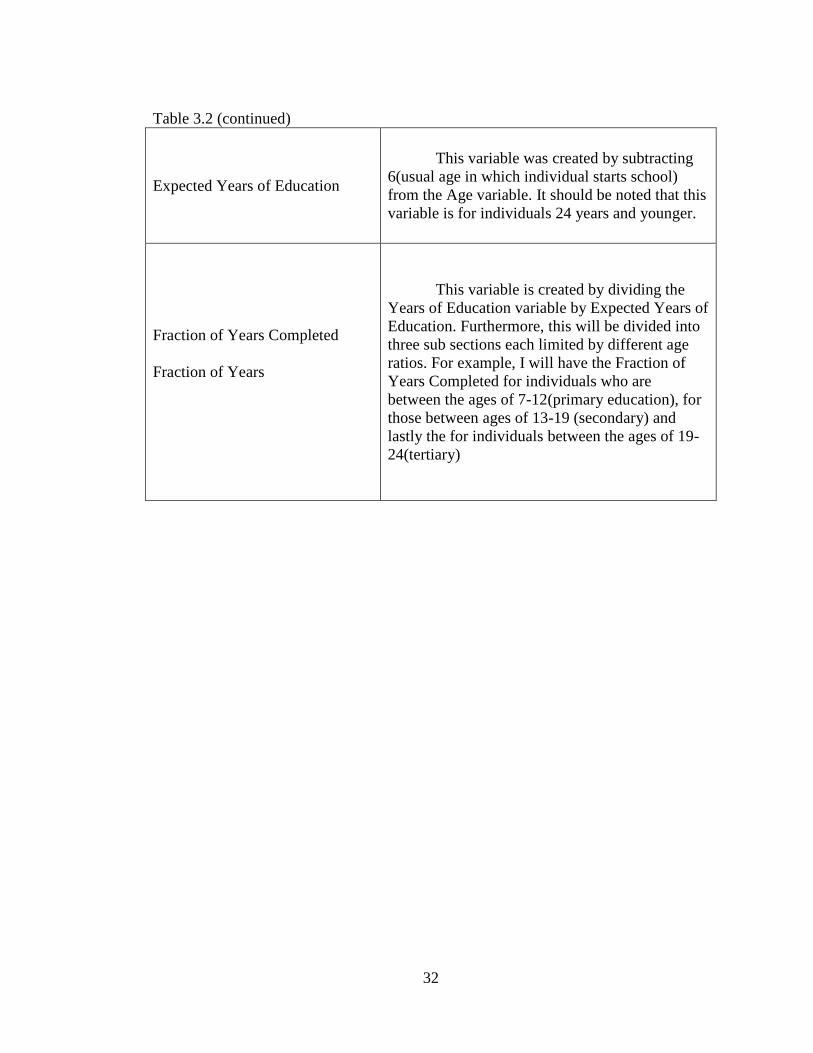
Expected Years of Education
This variable was created by subtracting6(usual age in which individual starts school)from the Age variable. It should be noted that thisvariable is for individuals 24 years and younger.
Fraction of Years Completed
Fraction of Years
This variable is created by dividing theYears of Education variable by Expected Years ofEducation. Furthermore, this will be divided intothree sub sections each limited by different ageratios. For example, I will have the Fraction ofYears Completed for individuals who arebetween the ages of 7-12(primary education), forthose between ages of 13-19 (secondary) andlastly the for individuals between the ages of 19-24(tertiary)

33
Chapter 4
METHODOLOGY
In this paper I will do several analyses to see the effects of remittances on
education and healthcare, as well as analyzing inequality by means of the Gini-
decomposition—and by regressing different percentile ratios on remittances. There are
several sets of equations that are being analyzed—all at regional and some of the
equations at the provincial level. The analysis in this paper is divided into three
distinct models. Models 1-A and 1-B look at the collapsed regional and provincial
level analysis respectively. Models 2-A and 2-B pertain to non-collapsed household
level data for both regional and provincial level analysis correspondingly. The Yearly
Models 1, 2, 3 and 4 will look at each individual year separately, while merely
focusing at the regional level. Models 3-A and 3-B look at the impact of remittances
on different percentile ratios at regional and provincial levels respectively. Finally,
Model 4-A (Table J.1 & J.2) pertain to the inequality analysis. In particular, Model 4-
A looks at the Gini-decomposition at a regional as well as provincial level for the
collapsed dataset. The equations for this paper are provided in the beginning of each
subsection. The Gini-Decomposition analysis does not require running a regression.
Instead, the analysis is contingent upon a user-written program (i.e. descogini). By

34
utilizing the “descogini” syntax in STATA, Lerman and Yitzhaki’s inequality
measurement is acquired. Following is some information related to the Models.
4.1 Models 1-A & 1-B
The equations relevant to Model 1-A & 1-B are as follows:
1. Yi=β0+β1REMIT+β2 (K) + β3Year + ui .
2. Yi=β0+β1REMIT+ B2 NRI+β3 (K) + β4Year + ui .
Here, Yi is a generic dependent variable. It takes the value of FYC for
different age groups, expenditure variables (Medical and Education), as well as
different percentile ratios (90th/10th, 10th/50th, and 50th/10th). Moreover, K is a general
term for Regions and Provinces. Equation 2 maintains the same values for the generic
terms; expect here we are also controlling for non-remittance income (NRI). As
mentioned earlier, it should be noted that this is the only occasion in which the
percentile ratios have been regressed.
Originally, the data pertaining to each year were cross-sectional. The data
related information about several regions and province, but at a single point in time.
Analyzing across regions with a single time reference could have an endogeniety (in
the form of omitted variable bias) problem. For example, looking at the 1999 data—
there is a possibility of an omitted variable that varies across regions or provinces, yet
correlated with remittances. A good example would be the migration patterns. A
poorer region might have a lower migration rate than that of a middle or high income
region. In doing so, I am not taking into account other factors that might influence
migration (better opportunity to migrate) more from certain regions, or the quality of
35
education in certain region might be higher than others. Therefore, I am omitting
factors such as education quality as well as better opportunities of migration from my
analysis. This will yield unconvincing and problematic results for the reasons
discussed earlier.
However, if I add the regions for different Years, then I can conduct a
cross-section/time-series analysis (pool the data), which will give me a better
representation of the effects of remittances on education. With this method, I will be
able to examine two different types of variations—interregional as well as
intratemporal. The interregional variation will give me the variation in average
education from one region to the next. The intertemporal will give me variation within
each region over time. Therefore, by having different observations about each region,
and looking at the effects of remittances within each region, we can hope to have rid
our analysis of omitted variable bias. There is however one catch. With the fixed-
effects regression one has to assume that other unobserved factors that might
simultaneously affect years of education and remittances of the regression are time-
invariant. This means that any shocks that could affect the level of migration (and
remittances), or the quality of education, if not accounted for could yield inadequate
results. To conclude, running a simple Ordinary Least Squares (OLS) might yield
incorrect results due to unobservable factors that are correlated with education, or
remittances in the regressions. Assuming the unobservable factors to be time-
invariant, the fixed-effects model will yield more consistent, and eliminate omitted
variable bias. The fixed-effects model pertains to Models 1-A and 1-B in this paper.
36
Models 1-A is essentially a difference-in-difference analysis of variation in
remittances across different and over span of 4 different years. The same is true for 1-
B, except using provinces and only 2 years (1999 and 2004) to examine the variation
in remittances. This isn’t the case with Models 2-A and 2-B.
4.2 Models 2-A & 2-B
Model 2-A compares household variations in remittances in the same year
and region. This is also the case for Model 2-B, except that it analyzes household
variations in remittances in the same year (only 1999 and 2004) and province (instead
of region). The equations relevant to Model 2-A & 3-B are as follows:
1. Yi=β0+β1REMIT+β2 (K) + β3Year + ui .
2. Yi=β0+β1REMIT+ B2 NRI+β3 (K) + β4Year + ui .
Here, Yi is a generic dependent variable. It takes the value of FYC for
different age groups and expenditure variables (Medical and Education). Moreover, K
is a general term for region and provinces. Equation 2 maintains the same values for
the generic terms; expect here we are also controlling for non-remittance income
(NRI). There are no percentile ration regressions done with Model 2.
There is one advantage that Model 2 has over Model 1. Model 2 accounts
for regional and yearly changes (i.e. shocks) which are also correlated with
remittances. For example, if there was a natural catastrophe (e.g. flooding) in a
specific region or province, then it will undoubtedly affect migration, which in turn
will influence remittances. This sort of a shock is absorbed by the analysis in Model

37
2. Nevertheless, Model 2 is not immune from omitted variable bias. There are strong
cultural differences among different households in the Philippines that certainly affect
their characteristics and are difficult to control. For example, in the mostly Muslim
populated region of ARMM, religious factors are taken into account when looking at
schooling. While the region is comprised of different religions, the vast majority of
them are Muslims. There is a vast number of Madaris (Islamic schools) in ARMM that
encourage emphasis on Islamic literature and Arabic studies. One of the major
migrant destinations for the Filipino migrants is the Middle East. It is very highly
likely the case that those who have knowledge of Arabic and are of the Muslim faith
will mostly be the ones who migrate. Thus, the likelihood of migration for the
Muslim household is higher than that of the non-Muslim family (especially if it is
migration to the Middle East). Furthermore, households differ by income. The
wealthier families will most have greater opportunities to migrate than the low income
families. Not only will the wealthier section of the population be able to migrate, but
are also most likely to have higher education (although not always the case). Thus, it is
very difficult to account for all these different household characteristics to get a better
measurement. For that reason, this is one disadvantage that Model 2 has over Model 1.
Model 2 cannot account for different household characteristics within regions and
provinces that could affect migration, and thus remittance patterns.

38
4.3 Our Expectations from the Equations
As mentioned earlier, for both of the Models, Yi represents a generic term
for the dependent variable. Thus there are several dependent variables for which
regressions were conducted. The first 5 regressions conducted look at the effects of
remittances on fraction of years completed for different ages. The next set of 5
regressions analyzes the same effect, although controlling for non-remittance income.
The next set of 4 regressions is related to education and health expenditures. These
regressions are pertinent to both Models 1 (collapsed) and 2 (non-collapsed
household), covering regional and provincial level analysis. Finally, we have 3
additional regressions to look at the impact of remittances on different percentile
rations (both regional and provincial level), but not accounting for non-remittance
income.
The expectations from the first 10 equations are one of an optimistic one.
Economic theory/anecdotal evidence suggest a positive impact of remittances on
education, even when controlling for non-remittance income. Remittances sent back
home should help the households in human capital investment. The Fraction of Years
Completed Per Capita (FYC) variable was selected as the dependent variable, since it
provides a better measurement of education attainment compared to Years of
Education. The FYC variable is further divided into 5 sub equations to account for
different age variations. Therefore, we will examine the effect of remittances on FYC
for individuals between the ages of 7 to 24 (Primary-Tertiary), 7 to 12(Primary), 13 to
18(Secondary), and finally 19 to 24(Tertiary).

39
We should see a positive relation between remittances and the FYC
variable for each age variation. Moreover, we should see a stronger relation between
remittances and primary level of education (ages 7 to12), as some studies have shown
(Dorantes and Pozo 2010). We should see a similar result, even when accounting for
non-remittance income. Moreover, the last four expenditure equations should further
clarify the impact of remittances (at least in terms of consumption). We should expect
remittances to have a positively linear relationship with education and healthcare
expenditures.
One would expect that a family receiving remittances will enable them to
buy school related supplies, or free up their income to be spent on education. This is
also similar in the case of healthcare. Remittances can affect health expenditures in
two ways. In the first instance, a family member might be in dire need of money for an
urgent medical issue, and thus the money sent from abroad could alleviate that
problem. This does not necessarily have to always be the case. Remittances sent back
could also be spent for normal medical expenditures, like buying drugs; although
drugs are not always bought to cure a sickness per se. Vitamins are also a form of
drug, yet they are mostly used to improve health and not necessarily cure sickness. In
this manner remittances can have both consumption and investment effects on health.
This is just to clarify that medical expenditures are not confined to one single activity.
Most of the equations pertain to the impact of remittances on education--with the
exception of equations 12 and 14. To account for the effect of remittances on
inequality, two methodologies have been used.

40
4.4 Inequality Analysis
The first analysis follows the Lerman and Yitzhaki (1985) measurement of
inequality. The Gini coefficient has been widely used to measure inequality in the
distribution of income, wealth, and expenditure. Using this literature, one can
decompose this measure to better understand the determinants of inequality.
According to Lerman and Yitzhaki, the Gini coefficient for total income, G, can be
shown as G=∑ R G S . Here Sk represents the share of component k in total
income, Gk shows the source Gini, which corresponds to the distribution of income
from source k, and Rk is the Gini correlation of income from source k with the
distribution of total income. There are three important issues to take into consideration
according to Stark, Taylor and Yitzhaki (1986). That is, the influence of any income
component on total income inequality depends upon:
1. The importance of income source with respect to total income (Sk)
2. The inequality distribution of the income source (Gk)
3. The correlation of income source with total income (Rk) (Taylor,Adams, Mora, and Lopez-Feldman 110-111)
In our case one of the income sources with respect to total income is
remittances, with the other one being salaries and wages. The 3 mechanisms discussed
earlier make it easy to estimate the influence of any income component (remittance in
our case) on total income inequality.
For instance, if I happen to have a large value for the remittances, so that
it constitutes a large share of the total income, then it may be possible that remittances

41
have a large impact on inequality. Conversely, if remittances constitute a small portion
of the total income, then it can be deduced that remittances do not have a large impact
on inequality. Although, if remittances is distributed equally (Gk=0), then regardless of
Sk, remittances will not affect inequality. If Sk and Gk happen to be large, that is
remittances are large and unequally distributed, remittances may either increase or
decrease inequality. For example, if the remittances are unequally distributed, and
flow towards household that are the top portion of income distribution, then
remittances will increase inequality. The inverse is also true. If the remittances are
unequally distributed, but tend to flow towards household that are in the lower portion
of the income bracket, then the remittances will have an equalizing affect.
Thus, according to Stark, Taylor and Yitzhaki, using the decomposition of
the Gini coefficient, one can estimate the effect that a 1 percent change in income
from remittances (source k), will have on total income inequality. The effect is given
by (SkRkGk/G)-Sk, where Sk, Rk, and Gk denote the source k share of income, Gini
correlation, and source Gini. An additional analysis of inequality was conducted by
regressing the different percentile ratios on remittances. This will allow for a
comparision of the top 90th percentile and the bottom 10th percentile, top 90th
percentile to median (50th percenilte), and finally 50th percentile to to the bottom 10th
percentile. The coefficeint estimates should provide some insight into the disparity
among different income distributions based on remittances. It should be noted that this
analysis has only been done for the collapsed data set for both regions (Model 3-A)
and provinces (Model 3-B). The following are the we get for the different models.

42
Chapter 5
RESULTS
5.1 Model 1-A & 1-B.
In the first ten equations, I examine the effects of remittances on the FYC
variable for different age groups. In Model 1-A, the sign of remittances is negative—
not the relationship we initially expected. The expectation was that of a positive
correlation between remittances and FYC. However looking at Model 1-A Table A.1,
coefficient estimate of remittances is negative (-10.6). This means that a 10 percent
increase in remittances above the mean (5908), will result in .63 percent decrease in
FYC for those between the ages of 7-24. But since the coefficient estimate is not
statistically significant at any level, we can conclude that regional remittances really
do not have any effect on regional changes in education. This is true across the board
for all FYC variables both at regional and provincial analysis. This is the case even
when controlling for non-remittance income. For example, in the provincial analysis
(Model 1-B) the coefficient estimate of FYC for ages 7 to 24 is (-
0.0000106*1,000,000=-10.6) is negative, although not statistically significant. This
means that even when growth of remittances differed across regions, growth of FYC
did not, at least statistically speaking. The FYC for all ages however, does not do a
fair job of explaining the impact of remittances on different age groups. Regardless,
43
remittances seem to have insignificant impact across the board for all the FYC
variables. Therefore, statistically speaking, remittances have not had a big impact on
education since 1999 (a very bold claim). However, when looking at the confidence
interval, we see that the value of 0 is bounded by the two extreme ends. For example,
looking at the extreme left (-50.6) and right (29.3) of the confidence interval (Model
1-A) for FYC (ages 7 to 24), a 10 percent increase in remittances lead to a decrease
and increase of -2.9 percent and 1.73 percent respectively. A similar pattern follows at
the provincial analysis. This means that Model 1 does not estimate a precise zero
effect.
5.2 Model 2-A & 2-B.
The coefficient estimates for the un-collapsed Models 2-A and 2-B are all
positive. This means that remittances have a positive impact on FYC for all the ages,
both at a regional and provincial level. For example a 10 percent increase in
remittances above the mean (688) will lead FYC (ages 7-24) to increase by .12 percent
for Model 2-A. Although positive, the dependent variable here includes a bigger age
range, and a better analysis would be to look at different age groups. This will enable
us to better examine the impact of remittances on FYC completed by looking in
specific age groups that usually attain education. The following are the results of the
effects of remittances on fraction of years completed for three sets of schooling: 7-24
(Primary-Tertiary) Primary (ages 7-12), Secondary (ages 13-18), and Tertiary (ages
19-24). The regressions in Model 2-A/2-B give us some expected results.

44
In Model 2-A, for individuals between the ages of 7-24, a 10 percent
increase in remittances will lead to an increase of .13 percent increase for FYC ages 7
to 24, a bit large compared to the regional (.12 percent). They are both significant at
99 percent level (p value of 0.00). Furthermore, at the regional level, a 10 percent
increase in remittances seem to have a larger affect on primary education compared to
secondary and tertiary (.22 percent primary vs. .06 percent secondary and .005 percent
tertiary). The results indicate that remittances sent back home are largely spent on
primary education. Remittances seem to have little if any pronounced effect on
tertiary schooling. This seems to conform to anecdotal evidence. Most of the
households that attain tertiary education will most likely be the households who can
afford it, and thus rely less on remittances and more on other sources of income.
These households tend to be in the upper-middle to higher part of the income
distribution. A similar pattern follows the provincial analysis, with primary education
being the prime recipient of remittances (.20 percent primary vs. .047 percent
secondary and .038 percent tertiary). Although the results seem to be congruent with
economic theory it is nevertheless important to control for non-remittance income.
This way we can truly get a good measure of the effects of remittances.
Again, the collapsed regional and provincial provide overwhelmingly
insignificant results—even when controlling for non-remittance income. Some
coefficient estimates for remittances are positive, while some are negative. Regardless,
they all exhibit a similar pattern—they are all insignificant. It should however be
mentioned that the two extremes of the confidence interval do have 0 bounded within
45
the interval. This means that the coefficient for remittance might have an impact on
different FYC variables, or it might have zero affects. This all depends on the value of
the extreme confidence interval. However, that is not the case with Model 2. Both at
the regional and provincial levels, controlling for non-remittance yield positive and
significant effects of remittances. As expected, the impact of remittances on all FYC
variables is not as pronounced when controlling for non-remittance income, except in
the case of primary education. For instance, the effect of remittances on FYC
variable for those between the ages of 13 and 18 is a bit lower when controlled for
non-remittance income (.06 percent vs. .05 percent increase) at the regional level. This
is also the case at the provincial level. Thus, overall we should also see a positive
impact on FYC from non-remittance income—and we do. A 10 percent increase in
non-remittance above the mean (14019) will lead to an astounding 21.1 percent
increase in primary education (ages 7-12), while it only increases tertiary education by
3.9 percent for Model 2-A. This further proves our point—in terms of education, most
of the remittances seem to flow towards primary education.
5.3 Yearly Models 1, 2, 3, & 4
The 2004 dataset is the only dataset that seems to give inconclusive results
for the non-expenditure equations. Although most of the signs of the coefficient
estimates are negative (except FYC 7-24), nevertheless, they are all insignificant. But
similar to Model 1, the confidence intervals range from -10 to 10. There is a possible
explanation for these uncommon effects. First of all, 2004 saw a very hotly contested

46
election year, in which for the first time the Overseas Absentee Voting Act of 2003
enabled overseas Filipinos to vote. Secondly, there was a huge tsunami in South Asia
which crippled the economies of many of the neighboring island countries (notably
Indonesia and Malaysia). This could very possibly have had a negative impact on the
Philippines economy as well. A 10 percent increase in remittances for 1999, 2007, and
2008 above mean (4340, 7866, 8453) will lead to increases of percent, .22 percent, and
.056 percent, and .48 percent for primary education—with all of the coefficients being
highly significant. Comparing the primary education with tertiary for each year, we
see an analogous trend as that of Model 2-A. The increase in tertiary education due to
remittances is lower than that of primary education; .0389 (1999), .0585 percent
(2007), .067 percent (2008), except for the year 2007. The results for the 2008 year do
look a little suspicious. It is very unlikely for remittance to have such a big impact on
primary education. The secondary education also seems to be a bit higher than tertiary,
but lower than primary. This is also the case when controlling for non-remittance
income.
Controlling for non-remittance income, a 10 percent increase in remittance
above mean for 1999, 2007, and 2008 years will lead to an increase of .21 (primary),
.056 percent (secondary), .051 percent (primary), .0347 percent (secondary), .45
percent (primary), and .12 percent (secondary) respectively. It is interesting to note
that aside from the 2004 year, remittances seem to have an increasingly positive effect
on education as the years progressed. A large volume of remittances seem to have
been spent on education in 2008, compared to 1999 (even when controlling for non-

47
remittance income). Of course, the regression does not take into account other
variables that could have affected education or remittances. Even so, the results seem
quite logical.
It is also important to see the effects of remittance on education and
healthcare expenditures to get a better perspective. The expenditure results will
include the results for collapsed (Models 1-A & 1-B), non-collapsed (Models 2-A &
2-B), and yearly datasets (1999, 2004, 2007, 2008). The regional and provincial
analysis will only be limited to Models 1 (collapsed dataset) and Models 2 (non-
collapsed household dataset), and not the yearly datasets.
5.4 Expenditure Results
For Model 1-A, remittances seem to have a positive effect on education
expenditure and medical expenditure. This is also the case when non-remittance
income is used as a control independent variable. However, only the education
expenditure coefficient is significant in both cases (.413 & .166 when controlling for
non-remittance income). Thus, we see a lesser impact of remittances on education
expenditure when controlling for non-remittance income. This is however only in the
regional analysis. For Model 1-B (provincial level), the opposite seems to be true.
Although the effect of remittances is positive and significant for both the education
and medical expenditure (.219 & .0765 respectively), the medical expenditure is the
only one that remains significant when controlled for non-remittance income (.061).
Thus, we have mixed effects of remittances on education and medical expenditures

48
when using the collapsed dataset. The results from Model 2-A and 2-B are more
consistent.
For Model 2-A, each peso of remittances results in increase of 8.5 percent
expenditure on education at the margin. Similarly each peso of remittances results in a
.0836 peso increase in education expenditure when controlling for non-remittance
income. This is also true for the medical expenditure. A 10 percent increase in
remittances will lead to an increase of approximately 3628 percent in health
expenditure for both controlled and uncontrolled effect of remittances. There seems to
be consistency in terms of the effects of remittances on education and medical
expenditures. This tendency is also seen in the yearly data sets, looking across
different regions.
In terms of regional analysis, 1999, 2004, 2007, and 2008 all show a
positive effect of remittances on education and medical expenditure. For example for
the year 1999, the education and medical expenditures have positive and significant
coefficients (.0284, .0229 respectively). That is also the case when controlling for
non-remittance income (.028 for education, .0224 for medical). For 2004, 2007, and
2008, education and expenditure coefficient estimates are positive and highly
significant for both controlled and uncontrolled non-remittance income. Tables E.3,
E.4, F.3, F.4, G.3, G.4, H.3, and H.4 provide the coefficient estimates of the
expenditure regressions. Aside from the regression analysis, it is also important to
take a look at the effect of remittances in terms of inequality. While remittances might
have a positive impact on education and health, it is important to see who benefits the

49
most from this impact. If most of the remittances help the higher income class, then
remittances do little in reducing poverty and inequality. The inequality
decomposition and regression of different percentile ratios give us a glance into the
inequality issue.
5.5 Inequality Analysis:
The two components of Total Income in a household in this paper are
given by salaries and wages, and remittances. The Gini coefficient for the remittances
component of total income is larger than that of the salaries and wages (.36 vs. .23).
One could conclude that remittances have a large impact on inequality. However, the
share of total income comprised by remittances is only 9 percent (Sk=.084). In
addition the correlation of remittances with total income is lower for remittances
compared to salaries and wages. In this case Sk and Rk are small, but Gk is large for
remittances compared to salaries and wages. The remittances could have an
inequality-reducing effect if the flow of remittances is geared towards the poor, and
not towards the wealthy households. The second analysis of inequality is done by
comparing different expenditure percentile ratios.
This analysis is done by regressing different percentile ratios on
remittances across regions and provinces (Models 3-A & 3-B). In another sense, this is
similar to Model 1-A and 1-B, in that it uses the collapsed dataset. Looking at Table
I.1 of Model 3-A, one can see that the disparity between the top 90th and the bottom
10th percentile is bigger than the other percentile ratios. The 90th to 10th percentile ratio

50
seems to be increasing by .07. This increase is less dramatic when looking at the 90th
to 50th percentile (.031 differences in 90th to 50th percentile ratio). The effect of
remittances further lessens when looking at the middle to bottom percentile ratios
(.0025 differences in 90th to 50th percentile ratio). The coefficient estimates are all
significantly different from zero, so our estimates are accurate. We see a big gap
between the top and the bottom portion of the income distribution, while the middle to
bottom is not as dramatic. We see an almost similar pattern in Model 3-B (provincial).
While the gap between the top and the bottom is even bigger than that of
the regional analysis (.072 increases in the percentile ratio difference), the gap
between top and the middle is smaller (.0282 increase in the percentile ratio
difference). It is interesting to look at the 50th to 10th percentiles. The negative
coefficient means that remittances actually decrease inequality between the middle
and the bottom class of the income distribution. The 50th to 10th percentile ratio seems
to be decreasing by .004. As expected, there exists a gap between the top and the
bottom portion of the income distribution, and remittances do seem to favor those who
are above the bottom percentile of the income distribution.

51
Chapter 6
SUMMARY & CONCLUSION
Most of the literatures related to remittances seem to paint a positive
picture of its effects on development. While remittances might not constitute a large
portion of a developed country’s economy, it plays a vital role in a developing nation’s
economy. In this paper the results indicate a positive impact of remittances on human
capital investment. That is particularly the case for individuals between the ages of 7-
12, who are earning primary education. The bulk of remittances seem to be directed
toward primary education as compared to secondary or tertiary. This is the case even
when controlling for non-remittance income. The 2004 Year dataset seems to yield
negative or insignificant coefficients estimates, which also affects the collapsed
datasets (both at a regional and provincial level). However, with the non-collapsed
datasets, the coefficient estimates seem to follow economic theory. The remittances
are positively correlated with education attainment with both uncontrolled and
controlled non-remittance regressions. Model 1 yields insignificant p-values.
Therefore, one cannot with certitude claim the validity or the invalidity of the
coefficient estimates in Model 1. Nevertheless, Model 1 is less biased than Model 2.
Model 1 takes into account any characteristics that could affect remittance variations

52
across regions, while Model 2 cannot account for household factors that are correlated
with remittances.
Additionally, when remittances are available, they seem to increase
education and medical expenditures, although not by a big magnitude. For example
for Model 2-A and 2-B,coefficient estimates for medical and education expenditures
are all positive and significant as shown in Tables C.3, C.4, D.3, and D.4. However,
there seems to be a disparity when it comes to inequality. The percentile ratios suggest
inequality among the top and the bottom income distribution. The income
decomposition seems to also suggest the same (Gini coefficient of remittances is
high), although the remittance share of total income seem to be less than salaries and
wages.
The results obtained from Models 2-A and 2-B also seem to be in line
with the studies done by Dorantes and Pozo. Most of the benefactors of remittances
seem to be younger siblings who are attending primary school. Additionally, the
analysis of percentile ratios suggests disparities among different distributions of
income, both at a regional and provincial level. This is also similar to the findings by
Taylor, that most of the remittances do not reach the poor families.
Overall remittances seem to play an important role in the Philippines, and
most likely many other developing nations. Remittances are a more stable form of
financial inflow, and tend to be immune to economic shocks. Although the paper
paints a positive picture of remittances on various factors of the Philippine society, we
still have to be cautious. The datasets for the regions and provinces are not consistent.
53
The lack of data for certain regions, such as Autonomous Region in Muslim
Mindanao, Caraga and Cordillera Administrative Region make it difficult to be
completely conclusive about the results. Additionally, there are many channels
through which remittances are sent and received. The actual amount of remittances is
most likely more than what is reported. Furthermore, as Skeldon (1997) points out
that most of the migrants do not belong to the poorest income distribution. In addition
to aspiration for a better life, migration involves physical, financial, and social risks
that many of the poorest in the least developed nations would most likely not
undertake. Thus, most of the migrants seem to come from lower-middle to upper-
middle incomes who have the necessary motivation, as well as the financially ability
to migrate. Thus remittances do not seem to help the poorest section of the society. In
fact most of the countries with high rates of emigration (Turkey, Mexico, and
Philippines) are no longer categorized as least developed. The fact is that migration
and remittance by themselves do not lead to development. To better exploit the full
potential of remittances, other constraints to development such as corruption, market
failures, access to credit, access to human capital (education, health), trade barriers, etc
need to be addressed. Over the years, the Philippines has addressed many of these
constraints, and have had significant improvements. Nevertheless, there is still room
for improvement in order to provide a suitable environment to fully exploit the
potentials of remittances.

54
REFERENCES
Amuedo-Dorantes, Catalina, and Susan Pozo. "Accounting for Remittance andMigration Effects on Children's Schooling." (2010): Print.
Ang, Alvin P. "Workers." DEGIT, Conference Papers. (2007): Print.
Asis, Maruja M.B. "The Philippines." Asian and Pacific Migration Journal.17.3-4 (2008): Print.
Burgess, R. and Haksar, H. (2005). “Migration and Foreign Remittances in thePhilippines.” IMF Working Paper WP/05/
Chami, Ralph, Connel Fullenkamp, and Samir Jahjah. "Are ImmigrantRemittance Flows a Source of Capital for Development?" PalgraveMacmillan Journals 52.1 (2005): 55-81. Web. 2 Jun 2011.<http://www.jstor.org/stable/30035948 .>.
Chauvet, Lisa, Flore Gubert, and Sandrine Mesle-Somps. "Are RemittancesMore Effective than Aid to Improve Child Health? An EmpiricalAssessment Using Inter and Intra-country Data." Annual BankConference on Development Economics. (2008): Print.
Chimhowu, Admos, Jenifer Piesse, and Caroline Pinder. The SocioeconomicImpact of Remittances on Poverty Reduction. Remittances:Development Impact and Future Prospects. Washington DC: The
Docquier, Frederic, Ousmane Faye, and Pierre Pestieau. "Is Migration a GoodSubstitute for Education Subsidies?" World Bank DevelopmentResearch Group. (2008): Print.
Edgar R., Rodriguez. "International Migrants' Remittances in the Philippines."Canadian Journal of Economics 29.Special (Apr 1996): S427-S432.Web. 2 Jun 2011. <http://www.jstor.org/stable/136081>.
Eduardo T., Gonzalez. "Does international migration induce human capitalinvestment and knowledge transfer? Evidence from the Philippines."Asian Center: University of the Philippines. (Undated): Print.
Edwards Cox, Alejandro, and Manuelita Ureta. "International migration,remittances, and schooling: evidence from El Salvador." Journal ofDevelopment Economics 72. (2003): 429-461. Web. 2 Jun 2011.<www.elsevier.com/locate/econbase>.

55
Fajnzylber, Pablo, and J. Humberto Lopez. Remittances and Development.Print.
Fayissa, Bichaka, and Christian Nsiah. "Can Remittances Spur EconomicGrowth and Development? Evidence from Latin American Countries(LACs)." (2010): Print.
Go, Stella P. "Remittances and International Labour Migration: Impact on thePhilippines." Philippine Migration Research Network. (Undated): Print.
Hildebrandt, Nicole. David J. McKenzie. “The Effects of Migration on childHealth in Mexico.” Economia: Project Muse. 6. (2005): 257-289.
International Bank for Reconstruction and Development, 83-99. Print.
Jorge, Valero-Gil. "Remittances and the household's expenditures on health."Munich Personal RePEc Archive. (2008)
Margarita R., Songco. "International labor migration and remittances in thePhilippines." National Economic and Development Authority. (Dec2009): Print.
McKenzie, David, and Marcin J. Sain. "Migration, Remittances, Poverty, andHuman Capital: Conceptual and empirical challenges." World BankPolicy Research Working Paper. (2007): Print.
Overseas Filipinos Workers. <http://overseasfilipinos.com/>.
Republic of Philippines National Statistics Office.<http://www.census.gov.ph>
Richard C., Jones. "Remittances and Inequality: A Question of Migration Stageand Geographic Scale." Economic Geography 74.1 (Jan 1998): 8-25.Web. 2 Jun 2011. <http://www.jstor.org/stable/144341 .>.
Skeldon, R (1997) Migration and Development: A Global Perspective(Harlow: Longman).
Stark, J., Edward, and Shlomo Yitzhaki. "Remittances and Inequality."Economic Journal 96.383 (Sep 1986): 722-740. Web. 2 Jun 2011.<http://www.jstor.org/stable/2232987>.
Taylor, J.Edward, Richard Adams, Jorge Mora, and Alejandro Lopez-Feldman."Remittances, Inequality and Poverty: Evidence from Rural Mexico."(2005): 110-111.
56
W. Stahl, Charles, and Fred Arnold. "Overseas Workers' Remittances in AsianDevelopment." International Migration Review 20.Temporary Worker(Winter 1986): 899-925. Web. 2 Jun 2011.<http://www.jstor.org/stable/2545742 >.
Yang, Dean, and Claudia A. Martinez. "Remittances and Poverty in Migrants'Home Areas: Evidence from the Philippines." Print.
Yang, Dean. (2008). International migration, remittances, and householdinvestment: Evidence from Philippine migrants’ exchange rate shocks,Economic Journal 118

57
Appendix A
MODEL 1-A (REGIONAL)
Table A.1 Effects of Remittances on Fraction of Years Completed:For Ages 7-1213-1819-247-24
(Primary) (Secondary) (Tertiary) (Primary-Tertiary)FYC_7_12 FYC_13_18 FYC_19_24 FYC_7_24
REMIT 2.2100 -0. 695 2.21 -10.6(26.900) (7.03) ( 2.80) (18.9)
Constant 3.710*** 1.000*** 0.581*** 2.114***
(0.188) (0.0492) (0.0223) (0.134)Standard errors in parentheses* p < 0.05, ** p < 0.01, *** p < 0.001REMITRemittances Received From AbroadCoefficients & Standard errors have been multiplied by 1 million, except for theConstant term.

58
Table A.2 Controlling For Non-Remittance Income Effects of Remittances onFraction of Years Completed:For Ages 7-1213-1819-247-24
(Primary) (Secondary) (Tertiary) (Primary-Tertiary)FYC_7_12 FYC_13_18 FYC_19_24 FYC_7_24
NRI -26 - 4.72 -1.10 -17.7(33.7) (6.53) (5.19) (15.5)
REMIT 12.3 1.93 2082 -0. 794(30.7) (6.65) (3.72) (20.9)
Constant 3.837*** 1.023*** 0.586*** 2.200***
(0.276) (0.0636) (0.0363) (0.144)* p < 0.05, ** p < 0.01, *** p < 0.001REMITRemittances Received From AbroadNRINon-Remittance IncomeCoefficients & Standard errors have been multiplied by 1 million, except for theConstant term.
Table A.3 Effect of Remittances on Education & Medical Expenditures
(1) (2)EDU_EXP MED_EXP
REMIT .4130* .0976(.1510) (.555)
Constant -1757.2 403.7(1395.9) (466.8)
Standard errors in parentheses* p < 0.05, ** p < 0.01, *** p < 0.001REMITRemittances Received From AbroadEDU_EXPEducation ExpenditureMED_EXP Medical Expenditure

59
Table A.4 Controlling For Non-Remittance IncomeEffect of Remittances on Education & Medical Expenditures
(1) (2)EDU_EXP MED_EXP
REMIT .166 * .0606(.734) (.0709)
NRI .443** .0665(.132) (.047)
Constant -3911.3** 80.63(1054.8) (374.2)
Standard errors in parentheses* p < 0.05, ** p < 0.01, *** p < 0.001REMITRemittances Received From AbroadNRINon-Remittance IncomeEDU_EXPEducation ExpenditureMED_EXP Medical Expenditure
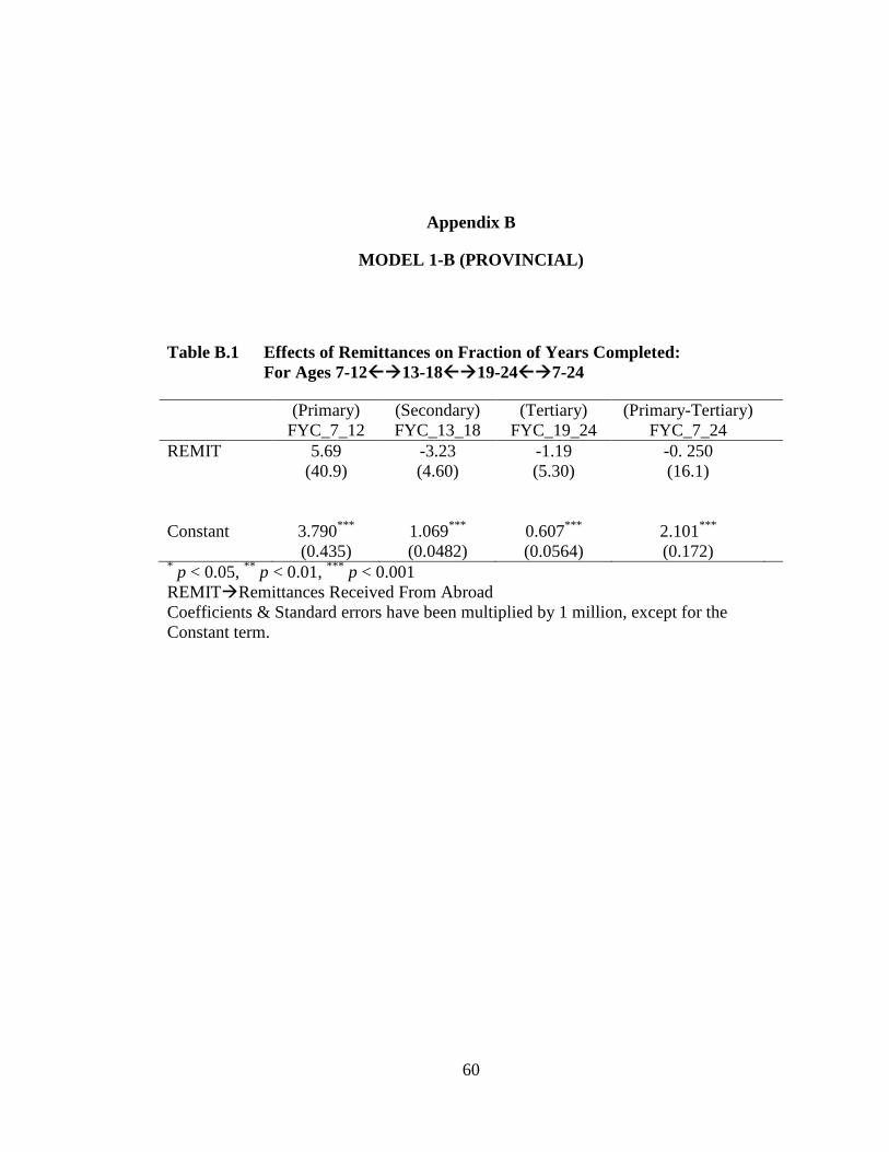
60
Appendix B
MODEL 1-B (PROVINCIAL)
Table B.1 Effects of Remittances on Fraction of Years Completed:For Ages 7-1213-1819-247-24
(Primary) (Secondary) (Tertiary) (Primary-Tertiary)FYC_7_12 FYC_13_18 FYC_19_24 FYC_7_24
REMIT 5.69 -3.23 -1.19 -0. 250(40.9) (4.60) (5.30) (16.1)
Constant 3.790*** 1.069*** 0.607*** 2.101***
(0.435) (0.0482) (0.0564) (0.172)* p < 0.05, ** p < 0.01, *** p < 0.001REMITRemittances Received From AbroadCoefficients & Standard errors have been multiplied by 1 million, except for theConstant term.

61
Table B.2 Controlling For Non-Remittance Income Effects of Remittances onFraction of Years Completed:For Ages 7-1213-1819-247-24
(Primary) (Secondary) (Tertiary) (Primary-Tertiary)FYC_7_12 FYC_13_18 FYC_19_24 FYC_7_24
NRI 19.9 2.87 2.88 10.6(28.8) (5.22) (3.51) (14.0)
REMIT -2.06 -4.34 -2.31 -4.36(47.8) (5.34) (6.14) (18.9)
Constant 3.692*** 1.055*** 0.592*** 2.049***
(0.376) (0.0510) (0.0492) (0.158)Standard errors in parentheses* p < 0.05, ** p < 0.01, *** p < 0.001REMITRemittances Received From AbroadNRINon-Remittance IncomeCoefficients & Standard errors have been multiplied by 1 million, except for theConstant term.
Table B.3 Effect of Remittances on Education & Medical Expenditures
(1) (2)EDU_EXP MED_EXP
REMIT 0.219* 0.0765*
(0.0957) (0.0307)
Constant 246.8 670.0*
(1054.9) (321.6)Standard errors in parentheses* p < 0.05, ** p < 0.01, *** p < 0.001REMITRemittances Received From AbroadEDU_EXPEducation ExpenditureMED_EXP Medical Expenditure

62
Table B.4 Controlling For Non-Remittance Income Effect of Remittances onEducation & Medical Expenditures
(1) (2)EDU_EXP MED_EXP
REMIT 0.0903 0.0615*
(0.0795) (0.0307)
NRI 0.332*** 0.0385(0.0595) (0.0450)
Constant -1390.1 480.2(835.9) (419.3)
Standard errors in parentheses* p < 0.05, ** p < 0.01, *** p < 0.001REMITRemittances Received From AbroadNRINon-Remittance IncomeEDU_EXPEducation ExpenditureMED_EXP Medical Expenditure
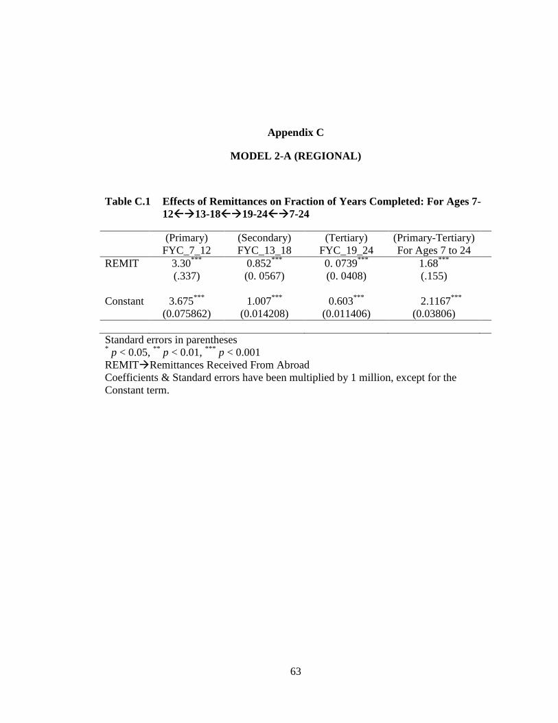
63
Appendix C
MODEL 2-A (REGIONAL)
Table C.1 Effects of Remittances on Fraction of Years Completed: For Ages 7-1213-1819-247-24
(Primary) (Secondary) (Tertiary) (Primary-Tertiary)FYC_7_12 FYC_13_18 FYC_19_24 For Ages 7 to 24
REMIT 3.30*** 0.852*** 0. 0739*** 1.68***
(.337) (0. 0567) (0. 0408) (.155)
Constant 3.675*** 1.007*** 0.603*** 2.1167***
(0.075862) (0.014208) (0.011406) (0.03806)
Standard errors in parentheses* p < 0.05, ** p < 0.01, *** p < 0.001REMITRemittances Received From AbroadCoefficients & Standard errors have been multiplied by 1 million, except for theConstant term.

64
Table C.2 Controlling For Non-Remittance Income Effects of Remittances onFraction of Years Completed: For Ages 7-1213-1819-247-24
(Primary) (Secondary) (Tertiary) (Primary-Tertiary)FYC_7_12 FYC_13_18 FYC_19_24 For Ages 7 to 24
NRI 15.1*** 3.74*** .278*** 7.39***
(0. 490) (0. 0802) (0. 0610) (0. 226)
REMIT 3.0*** 0. 810*** 0. 727*** 1.59***
(0. 336) (0. 0560) (0. 040) (0. 154)
Constant 3.529*** 0.970*** 0.574*** 2.0428***
(0.07562) (0.01404) (0.01122) (0.03804)Standard errors in parentheses* p < 0.05, ** p < 0.01, *** p < 0.001REMITRemittances Received From AbroadNRINon-Remittance IncomeCoefficients & Standard errors have been multiplied by 1 million, except for theConstant term.
Table C.3 Effect of Remittances on Education & Medical Expenditures
(1) (2)EDU_EXP MED_EXP
REMIT 0.0859*** 0.07044***
(0.00044) (0.000586)
Constant 1023.266*** 654.27***
(110.364) (145.69)Standard errors in parentheses* p < 0.05, ** p < 0.01, *** p < 0.001REMITRemittances Received From AbroadEDU_EXPEducation ExpenditureMED_EXP Medical Expenditure
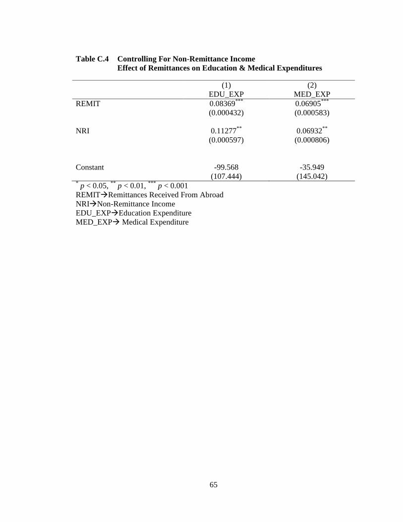
65
Table C.4 Controlling For Non-Remittance IncomeEffect of Remittances on Education & Medical Expenditures
(1) (2)EDU_EXP MED_EXP
REMIT 0.08369*** 0.06905***
(0.000432) (0.000583)
NRI 0.11277** 0.06932**
(0.000597) (0.000806)
Constant -99.568 -35.949(107.444) (145.042)
* p < 0.05, ** p < 0.01, *** p < 0.001REMITRemittances Received From AbroadNRINon-Remittance IncomeEDU_EXPEducation ExpenditureMED_EXP Medical Expenditure
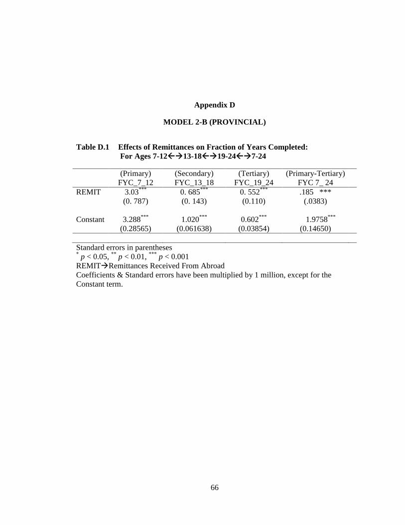
66
Appendix D
MODEL 2-B (PROVINCIAL)
Table D.1 Effects of Remittances on Fraction of Years Completed:For Ages 7-1213-1819-247-24
(Primary) (Secondary) (Tertiary) (Primary-Tertiary)FYC_7_12 FYC_13_18 FYC_19_24 FYC 7_ 24
REMIT 3.03*** 0. 685*** 0. 552*** .185 ***(0. 787) (0. 143) (0.110) (.0383)
Constant 3.288*** 1.020*** 0.602*** 1.9758***
(0.28565) (0.061638) (0.03854) (0.14650)
Standard errors in parentheses* p < 0.05, ** p < 0.01, *** p < 0.001REMITRemittances Received From AbroadCoefficients & Standard errors have been multiplied by 1 million, except for theConstant term.

67
Table D.2 Controlling For Non-Remittance Income Effects of Remittances onFraction of Years Completed:For Ages 7-1213-1819-247-24
(Primary) (Secondary) (Tertiary) (Primary-Tertiary)FYC_7_12 FYC_13_18 FYC_19_24 For Ages 7 to 24
NRI 20.6*** 3.98*** 2.88*** 9.928***
(1.04) (0.000000163) (0. 0124) (0. 466)
REMIT 2.74*** 0. 664*** 0. 554*** 1.78***
(0. 783) (0. 141) (0. 108) (0. 383)
Constant 3.130*** 0.987*** 0.578*** 1.90095***
(0.28424) (0.06106) (0.038087) (0.146229)Standard errors in parentheses* p < 0.05, ** p < 0.01, *** p < 0.001REMITRemittances Received From AbroadNRINon-Remittance IncomeCoefficients & Standard errors have been multiplied by 1 million, except for theConstant term.
Table D.3 Effect of Remittances on Education & Medical Expenditures
(1) (2)EDU_EXP MED_EXP
REMIT 0.0423*** 0.02665***
(0.00076) (0.001244)
Constant 1692.307*** 722.79(298.398) (488.159)
Standard errors in parentheses* p < 0.05, ** p < 0.01, *** p < 0.001REMITRemittances Received From AbroadEDU_EXPEducation ExpenditureMED_EXP Medical Expenditure

68
Table D.4 Controlling For Non-Remittance IncomeEffect of Remittances on Education & Medical Expenditures
(1) (2)EDU_EXP MED_EXP
REMIT 0.041883*** 0.0262836***
(0.000754) (0.0012413)
NRI 0.05749** 0.04954**
(0.0009299) (0.0015304)
Constant 1219.686*** 315.5909(296.047) (487.2147)
* p < 0.05, ** p < 0.01, *** p < 0.001REMITRemittances Received From AbroadNRINon-Remittance IncomeEDU_EXPEducation ExpenditureMED_EXP Medical Expenditure

69
Appendix E
1999 (REGIONAL)
Table E.1 Effects of Remittances on Fraction of Years Completed:For Ages 7-1213-1819-247-24
(Primary) (Secondary) (Tertiary) (Primary-Tertiary)FYC_7_12 FYC_13_18 FYC_19_24 For Ages 7 to 24
REMIT 5.28*** 1.33*** 0.897*** 3.05***
(1.25) (0. 238) (0. 163) (0. 735)
Constant 3.661*** 1.004*** 0.602*** 2.106***
(0.00964) (0.00196) (0.00133) (0.00587)Standard errors in parentheses* p < 0.05, ** p < 0.01, *** p < 0.001REMITRemittances Received From AbroadCoefficients & Standard errors have been multiplied by 1 million, except for theConstant term.
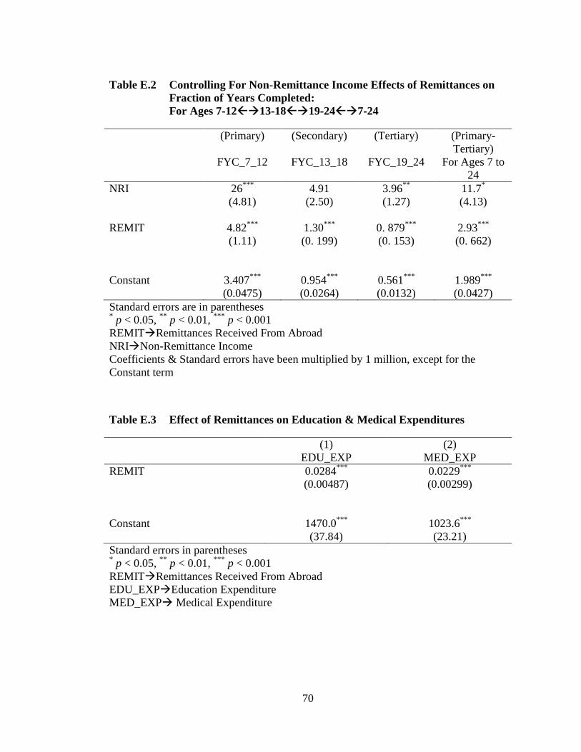
70
Table E.2 Controlling For Non-Remittance Income Effects of Remittances onFraction of Years Completed:For Ages 7-1213-1819-247-24
(Primary) (Secondary) (Tertiary) (Primary-Tertiary)
FYC_7_12 FYC_13_18 FYC_19_24 For Ages 7 to24
NRI 26*** 4.91 3.96** 11.7*
(4.81) (2.50) (1.27) (4.13)
REMIT 4.82*** 1.30*** 0. 879*** 2.93***
(1.11) (0. 199) (0. 153) (0. 662)
Constant 3.407*** 0.954*** 0.561*** 1.989***
(0.0475) (0.0264) (0.0132) (0.0427)Standard errors are in parentheses* p < 0.05, ** p < 0.01, *** p < 0.001REMITRemittances Received From AbroadNRINon-Remittance IncomeCoefficients & Standard errors have been multiplied by 1 million, except for theConstant term
Table E.3 Effect of Remittances on Education & Medical Expenditures
(1) (2)EDU_EXP MED_EXP
REMIT 0.0284*** 0.0229***
(0.00487) (0.00299)
Constant 1470.0*** 1023.6***
(37.84) (23.21)Standard errors in parentheses* p < 0.05, ** p < 0.01, *** p < 0.001REMITRemittances Received From AbroadEDU_EXPEducation ExpenditureMED_EXP Medical Expenditure
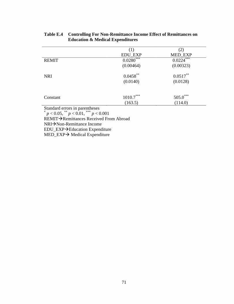
71
Table E.4 Controlling For Non-Remittance Income Effect of Remittances onEducation & Medical Expenditures
(1) (2)EDU_EXP MED_EXP
REMIT 0.0280*** 0.0224***
(0.00464) (0.00323)
NRI 0.0458** 0.0517**
(0.0140) (0.0128)
Constant 1010.7*** 505.0***
(163.5) (114.0)Standard errors in parentheses* p < 0.05, ** p < 0.01, *** p < 0.001REMITRemittances Received From AbroadNRINon-Remittance IncomeEDU_EXPEducation ExpenditureMED_EXP Medical Expenditure

72
Appendix F
2004 (REGIONAL)
Table F.1 Effects of Remittances on Fraction of Years Completed: For Ages 7-1213-1819-247-24
(Primary) (Secondary) (Tertiary) (Primary-Tertiary)FYC_7_12 FYC_13_18 FYC_19_24 For Ages 7 to 24
REMIT -.0068 -0. 414 -.00598 .00889(0. 530) (0.209) (0. 231) (0. 375)
Constant 4.191*** 1.134*** 0.663*** 2.234***
(0.00505) (0.00170) (0.00179) (0.00322)Standard errors in parentheses* p < 0.05, ** p < 0.01, *** p < 0.001REMITRemittances Received From AbroadCoefficients & Standard errors have been multiplied by 1 million, except for theConstant term

73
Table F.2 Controlling For Non-Remittance Income Effects of Remittances onFraction of Years Completed: For Ages 7-1213-1819-247-24
(Primary) (Secondary) (Tertiary) (Primary-Tertiary)FYC_7_12 FYC_13_18 FYC_19_24 For Ages 7 to 24
NRI 2.84 0. 112 -0. 196 1.31(2.26) (0. 293) (0. 269) (1.05)
REMIT -0.000000116 -0. 416 -.00589 7.06e-08(0.000000535) (0. 211) (0. 231) (0.000000375)
2.219***
Constant 4.155*** 1.133*** 0.665*** (0.0133)(0.0296) (0.00300) (0.00397) (2)
Standard errors in parentheses* p < 0.05, ** p < 0.01, *** p < 0.001REMITRemittances Received From AbroadNRINon-Remittance IncomeCoefficients & Standard errors have been multiplied by 1 million, except for theConstant term
Table F.3 Effect of Remittances on Education & Medical Expenditures
(1) (2)Education Medical Care
REMIT 0.0665*** 0.0334***
(0.00415) (0.00663)Constant 1628.4*** 962.5***
(38.50) (61.42)Standard errors in parentheses* p < 0.05, ** p < 0.01, *** p < 0.001REMITRemittances Received From AbroadEDU_EXPEducation ExpenditureMED_EXP Medical Expenditure
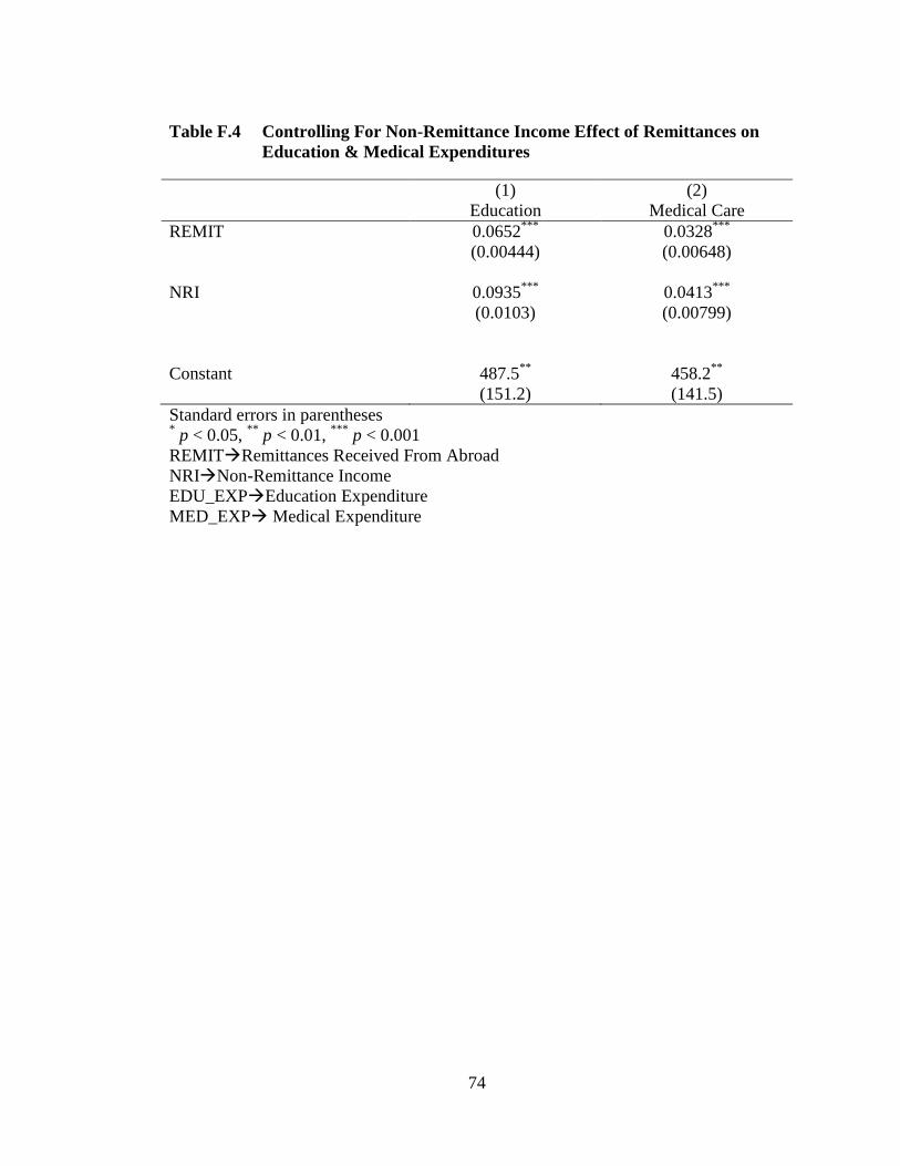
74
Table F.4 Controlling For Non-Remittance Income Effect of Remittances onEducation & Medical Expenditures
(1) (2)Education Medical Care
REMIT 0.0652*** 0.0328***
(0.00444) (0.00648)
NRI 0.0935*** 0.0413***
(0.0103) (0.00799)
Constant 487.5** 458.2**
(151.2) (141.5)Standard errors in parentheses* p < 0.05, ** p < 0.01, *** p < 0.001REMITRemittances Received From AbroadNRINon-Remittance IncomeEDU_EXPEducation ExpenditureMED_EXP Medical Expenditure

75
Appendix G
2007 (REGIONAL)
Table G.1 Effects of Remittances on Fraction of Years Completed: For Ages 7-1213-1819-247-24
(Primary) (Secondary) (Tertiary) (Primary-Tertiary)
FYC_7_12 FYC_13_18 FYC_19_24 FYC_7_24REMIT 0. 718*** 0. 463*** 0. 743*** 0. 319**
(.00789) (.00644) (.00894) (.00870)
Constant 1.934*** 1.188*** 0.875*** 1.399***
(0.000892) (0.000761) (0.00129) (0.00107)Standard errors in parentheses* p < 0.05, ** p < 0.01, *** p < 0.001REMITRemittances Received From AbroadCoefficients & Standard errors have been multiplied by 1 million, except for theConstant term

76
Table G.2 Controlling For Non-Remittance Income Effects of Remittances onFraction of Years Completed: For Ages 7-1213-1819-247-24
(Primary) (Secondary) (Tertiary) (Primary-Tertiary)FYC_7_12 FYC_13_18 FYC_19_24 For Ages 7 to 24
NRI 4.94*** 2.06** 1.99* 0. 560(1.01) (0. 553) (0. 690) (0. 440)
REMIT 0. 642*** 0. 441*** 0.739*** 0. 313**
(.00828) (.00567) (.00748) (.00832)
Constant 1.887*** 1.165*** 0.846*** 1.393***
(0.00955) (0.00634) (0.0101) (0.00554)Standard errors in parentheses* p < 0.05, ** p < 0.01, *** p < 0.001REMITRemittances Received From AbroadNRINon-Remittance IncomeCoefficients & Standard errors have been multiplied by 1 million, except for theConstant term
Table G.3 Effect of Remittances on Education & Medical Expenditures
(1) (2)Education Medical Care
REMIT 0.110*** 0.0633***
(0.0148) (0.00923)
Constant 1855.8*** 1034.7***
(185.3) (115.9)Standard errors in parentheses* p < 0.05, ** p < 0.01, *** p < 0.001REMITRemittances Received From AbroadEDU_EXPEducation ExpenditureMED_EXP Medical Expenditure

77
Table G.4 Controlling For Non-Remittance Income Effect of Remittances onEducation & Medical Expenditures
(1) (2)Education Medical Care
REMIT 0.107*** 0.0622***
(0.0153) (0.00947)
NRI 0.146*** 0.0677***
(0.0131) (0.0146)
Constant 52.84 200.3(300.8) (216.8)
Standard errors in parentheses* p < 0.05, ** p < 0.01, *** p < 0.001REMITRemittances Received From AbroadNRINon-Remittance IncomeEDU_EXPEducation ExpenditureMED_EXP Medical Expenditure

78
Appendix H
2008 (REGIONAL)
Table H.1 Effects of Remittances on Fraction of Years Completed: For Ages 7-1213-1819-247-24
(Primary) (Secondary) (Tertiary) (Primary-Tertiary)FYC_7_12 FYC_13_18 FYC_19_24 For Ages 7 to 24
REMIT 5.73*** 1.52*** 0. 797*** 3.09***
(1.18) (0. 182) (.00882) (0. 513)
Constant 4.253*** 1.160*** 0.691*** 2.224***
(0.0129) (0.00198) (0.00110) (0.00578)Standard errors in parentheses* p < 0.05, ** p < 0.01, *** p < 0.001REMITRemittances Received From AbroadCoefficients & Standard errors have been multiplied by 1 million, except for theConstant term
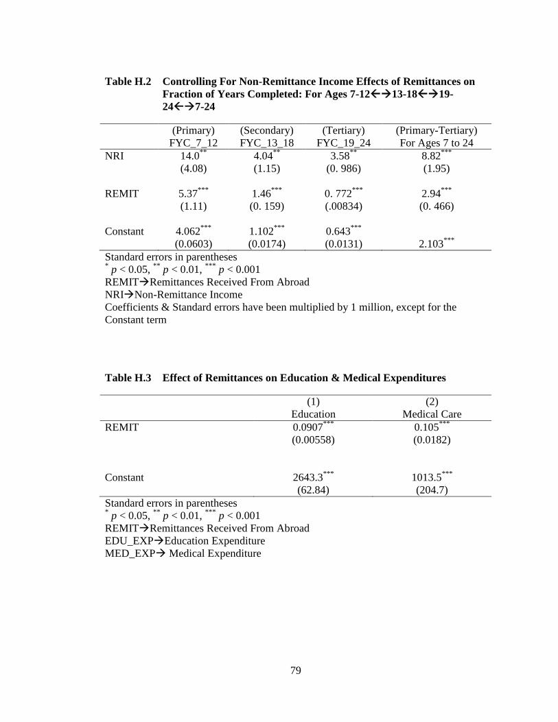
79
Table H.2 Controlling For Non-Remittance Income Effects of Remittances onFraction of Years Completed: For Ages 7-1213-1819-247-24
(Primary) (Secondary) (Tertiary) (Primary-Tertiary)FYC_7_12 FYC_13_18 FYC_19_24 For Ages 7 to 24
NRI 14.0** 4.04** 3.58** 8.82***
(4.08) (1.15) (0. 986) (1.95)
REMIT 5.37*** 1.46*** 0. 772*** 2.94***
(1.11) (0. 159) (.00834) (0. 466)
Constant 4.062*** 1.102*** 0.643***
(0.0603) (0.0174) (0.0131) 2.103***
Standard errors in parentheses* p < 0.05, ** p < 0.01, *** p < 0.001REMITRemittances Received From AbroadNRINon-Remittance IncomeCoefficients & Standard errors have been multiplied by 1 million, except for theConstant term
Table H.3 Effect of Remittances on Education & Medical Expenditures
(1) (2)Education Medical Care
REMIT 0.0907*** 0.105***
(0.00558) (0.0182)
Constant 2643.3*** 1013.5***
(62.84) (204.7)Standard errors in parentheses* p < 0.05, ** p < 0.01, *** p < 0.001REMITRemittances Received From AbroadEDU_EXPEducation ExpenditureMED_EXP Medical Expenditure

80
Table H.4 Controlling For Non-Remittance Income Effect of Remittances onEducation & Medical Expenditures
(1) (2)Education Medical Care
REMIT 0.0868*** 0.103***
(0.00605) (0.0177)
NRI 0.130*** 0.0855***
(0.0108) (0.0187)
Constant 885.2*** -138.5(168.0) (270.9)
Standard errors in parentheses* p < 0.05, ** p < 0.01, *** p < 0.001REMITRemittances Received From AbroadNRINon-Remittance IncomeEDU_EXPEducation ExpenditureMED_EXP Medical Expenditure

81
Appendix I
MODEL 3-A (REGIONAL/PROVINCIAL)
Table I.1 Regional Effects of Remittances on Different Percentile Ratios
(Top-Bottom) (Top-Middle) (Middle-Bottom)90th to 10thPercentile
90th to 50thPercentile
50th to 10thPercentile
REMIT 119* 52.7** 4.07(41.7) (17.0) (1906)
Constant 4.161*** 2.099*** 1.995***
(0.350) (0.155) (0.167)Standard errors in parentheses* p < 0.05, ** p < 0.01, *** p < 0.001REMITRemittances Received From Abroad
Table I.2 Provincial Effects of Remittances on Different Percentile Ratios
(Top-Bottom) (Top-Middle) (Middle-Bottom)90th to 10thPercentile
90th to 50thPercentile
50th to 10thPercentile
REMIT 122.9 *** 47.9 *** -6.81***
(36.3) (14.3 ) (1.88)
Constant 5.303 *** 2.734*** 0.381***
(.6397) (.252) (0.033)Standard errors in parentheses* p < 0.05, ** p < 0.01, *** p < 0.001REMITRemittances Received From Abroad
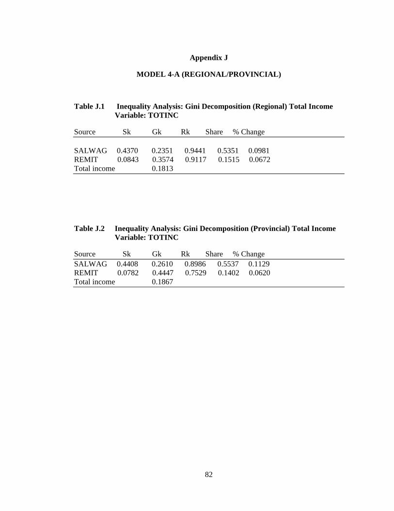
82
Appendix J
MODEL 4-A (REGIONAL/PROVINCIAL)
Table J.1 Inequality Analysis: Gini Decomposition (Regional) Total IncomeVariable: TOTINC
Source Sk Gk Rk Share % Change
SALWAG 0.4370 0.2351 0.9441 0.5351 0.0981REMIT 0.0843 0.3574 0.9117 0.1515 0.0672Total income 0.1813
Table J.2 Inequality Analysis: Gini Decomposition (Provincial) Total IncomeVariable: TOTINC
Source Sk Gk Rk Share % ChangeSALWAG 0.4408 0.2610 0.8986 0.5537 0.1129REMIT 0.0782 0.4447 0.7529 0.1402 0.0620Total income 0.1867