MUSIC STRUCTURE ANALYSIS BASED ON AN LSTM-HSMM …

MUSIC STRUCTURE ANALYSISBASED ON AN LSTM-HSMM HYBRID MODEL

Go Shibata Ryo Nishikimi Kazuyoshi YoshiiGraduate School of Informatics, Kyoto University, Japan

{gshibata, nishikimi, yoshii}@sap.ist.i.kyoto-u.ac.jp

ABSTRACT

This paper describes a statistical music structure analysismethod that splits an audio signal of popular music intomusically meaningful sections at the beat level and clas-sifies them into predefined categories such as intro, verse,and chorus, where beat times are assumed to be estimatedin advance. A basic approach to this task is to train a recur-rent neural network (e.g., long short-term memory (LSTM)network) that directly predicts section labels from acous-tic features. This approach, however, suffers from fre-quent musically unnatural label switching because the ho-mogeneity, repetitiveness, and duration regularity of musi-cal sections are hard to represent explicitly in the networkarchitecture. To solve this problem, we formulate a unifiedhidden semi-Markov model (HSMM) that represents thegenerative process of homogeneous mel-frequency cepstrumcoefficients, repetitive chroma features, and mel spectrafrom section labels, where the emission probabilities ofmel spectra are computed from the posterior probabilitiesof section labels predicted by an LSTM. Given these acous-tic features, the most likely label sequence can be esti-mated with Viterbi decoding. The experimental resultsshow that the proposed LSTM-HSMM hybrid model out-performed a conventional HSMM.

1. INTRODUCTION

Music structure analysis is the fundamental task in the fieldof music information retrieval (MIR) [1] because the mu-sical structure, which consists of several sections includingintro, verse, bridge, and chorus, is one of the most impor-tant elements of popular music. Most studies have tackledthe segmentation task, which splits audio signals into sev-eral sections [2–12], the clustering task, which categorizessuch sections into several classes [13–23], or both. Beyondthe clustering task that gives arbitrary labels such as “A”and “B” to detected sections, we tackle the labeling taskthat gives concrete labels such as “verse A”, “verse B”, and“chorus” [4,24] because such musically meaningful labelsare useful for playback navigation [25]. Because section

c© G. Shibata, R. Nishikimi, and K. Yoshii. Licensed undera Creative Commons Attribution 4.0 International License (CC BY 4.0).Attribution: G. Shibata, R. Nishikimi, and K. Yoshii, “Music structureanalysis based on an LSTM-HSMM hybrid model”, in Proc. of the 21stInt. Society for Music Information Retrieval Conf., Montréal, Canada,2020.

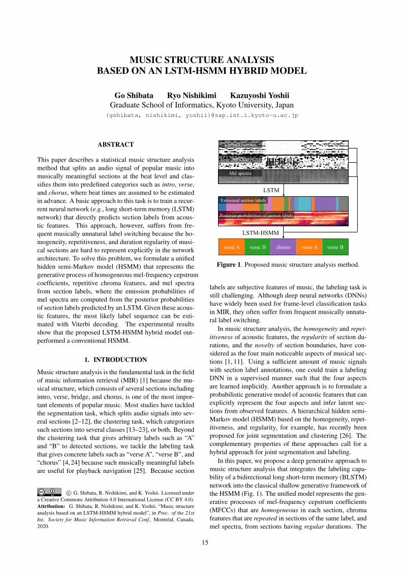
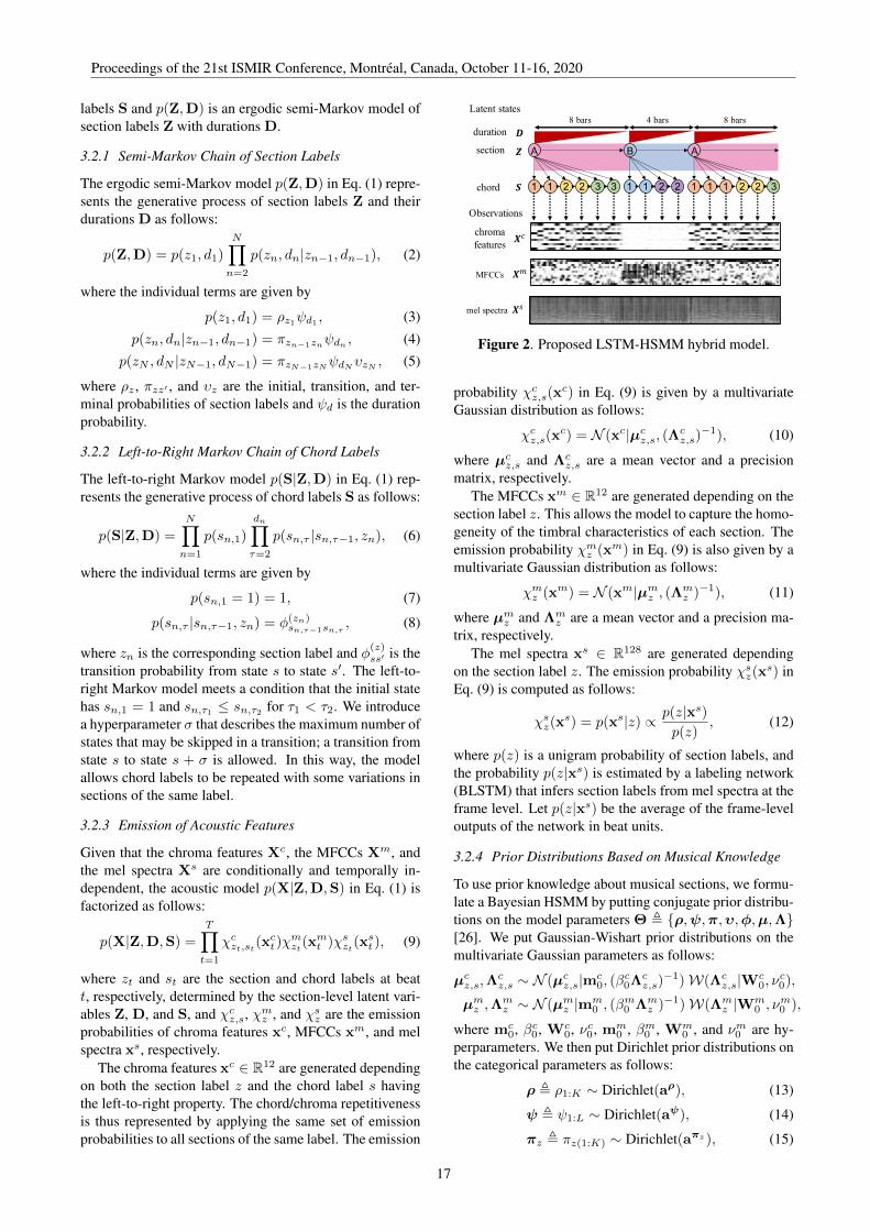
Chroma features

MFCCs

Mel spectra

Posterior probabilities of section labels

Estimated section labels

verse A verse B chorus verse A verse B

LSTM

LSTM-HSMM

Figure 1. Proposed music structure analysis method.

labels are subjective features of music, the labeling task isstill challenging. Although deep neural networks (DNNs)have widely been used for frame-level classification tasksin MIR, they often suffer from frequent musically unnatu-ral label switching.

In music structure analysis, the homogeneity and repet-itiveness of acoustic features, the regularity of section du-rations, and the novelty of section boundaries, have con-sidered as the four main noticeable aspects of musical sec-tions [1, 11]. Using a sufficient amount of music signalswith section label annotations, one could train a labelingDNN in a supervised manner such that the four aspectsare learned implicitly. Another approach is to formulate aprobabilistic generative model of acoustic features that canexplicitly represent the four aspects and infer latent sec-tions from observed features. A hierarchical hidden semi-Markov model (HSMM) based on the homogeneity, repet-itiveness, and regularity, for example, has recently beenproposed for joint segmentation and clustering [26]. Thecomplementary properties of these approaches call for ahybrid approach for joint segmentation and labeling.

In this paper, we propose a deep generative approach tomusic structure analysis that integrates the labeling capa-bility of a bidirectional long short-term memory (BLSTM)network into the classical shallow generative framework ofthe HSMM (Fig. 1). The unified model represents the gen-erative processes of mel-frequency cepstrum coefficients(MFCCs) that are homogeneous in each section, chromafeatures that are repeated in sections of the same label, andmel spectra, from sections having regular durations. The

15

BLSTM network that estimates section labels from melspectra at the frame level is trained in a supervised man-ner. The emission probabilities of mel spectra from sec-tions are computed at run-time by referring to the posteriorprobabilities of section labels estimated by the network andthe empirical prior distributions of section labels. Givenacoustic features, the latent section sequence as well asthe initial, transition, duration, and terminal probabilitiesof sections are estimated in a Bayesian manner with Gibbssampling followed by Viterbi decoding, where the latentsection sequence is initialized by the network to avoid badlocal optima.

The main contribution of this paper is to propose a sta-tistical joint segmentation and labeling method based on aBayesian LSTM-HSMM hybrid model that can be adaptedto each musical piece. Because the statistical characteris-tics of sections are specific to each musical piece, Bayesianinference based on the empirical prior distributions of thosecharacteristics plays an essential role for improving theperformance of music structure analysis. We experimen-tally show that the proposed method significantly outper-formed a cascade model using the labeling results of theBLSTM in the post-processing and an LSTM-HSMM mod-el using only Viterbi decoding.

2. RELATED WORK

This section reviews music structure analysis methods interms of segmentation, clustering, and labeling.

2.1 Segmentation

In the segmentation task, the novelty plays a central role.Foote [2] detected peaks from a novelty curve obtained byconvoluting a checkerboard kernel with the diagonal el-ements of a self-similarity matrix (SSM). Jensen [3] de-tected section boundaries such that a homogeneity- andnovelty-aware cost function is minimized. Goto [4] andSerrà et al. [5] proposed novelty curves computed from lagSSMs showing repetitions as vertical lines. These meth-ods were integrated for better segmentation [6] and themethod [5] was extended for clustering [7]. Recently, Ull-rich et al. [8] proposed a supervised method based on aconvolutional neural network, which was extended to dealwith coarse and fine boundary annotations [9]. Smith et al.[10] emphasized the importance of considering the regu-larity in the main analysis step, not in the post-processingstep. Sargent et al. [11] focused on the regularity to favorcomparable-size sections. Maezawa [12] used an LSTMnetwork based on a cost function considering the homo-geneity, repetitiveness, novelty, and regularity.

2.2 Clustering and Labeling

Cooper et al. [13] sequentially performed segmentation [2]and clustering based on intra- and inter-section character-istics. Goodwin et al. [14] efficiently detected off-diagonalstripes as repetitions from an SSM using dynamic pro-gramming. To deal with the repetitiveness and homogene-ity, Grohganz et al. [15] converted a repetitiveness-aware

SSM with off-diagonal stripes into a homogeneity-awareSSM with a block-diagonal structure. Nieto et al. [16] useda convex variant of nonnegative matrix factorization forsegmentation and clustering. McFee et al. [17] encodedrepetitive structures into a graph and performed spectralclustering for graph partitioning. Cheng et al. [18] con-verted a path-enhanced SSM into a block-enhanced SSMusing nonnegative matrix factor deconvolution as in [15].

Several studies have taken a statistical approach basedon generative models for joint segmentation and cluster-ing. Aucouturier et al. [19] used a standard HMM. Levyet al. [20] proposed an HSMM based on the regularity ofsection durations. Ren et al. [21] proposed a nonparamet-ric Bayesian HMM that can estimate an appropriate num-ber of sections. Barrington et al. [22] proposed a nonpara-metric Bayesian switching linear dynamical system (LDS)that has the ability of automatic model complexity control.

Only a few studies have attempted to estimate musicallymeaningful labels. Maddage et al. [27] proposed a label-ing method based on a typical music structure and the roleof each section. Paulus et al. [24] performed segmenta-tion, clustering, and labeling using a probabilistic fitnessmeasure for the N-grams of sections.

3. PROPOSED METHOD

This section describes the proposed method for music struc-ture analysis.

3.1 Problem Specification

The task we tackle in this paper is specified as follows:

Assumption: The beat times of a target music audio areestimated in advance by a beat tracking method [28].Input: Beat-level chroma features Xc , xc1:T (xct ∈ R12),MFCCs Xm , xm1:T (xmt ∈ R12), and mel spectra Xs ,xs1:T (xst ∈ R128) obtained from the target music signal,where T is the number of beats (quarter notes).Output: Section labels Z , z1:N (zn ∈ {1, . . . ,K}) withdurations D , d1:N (dn ∈ {1, . . . , L}), where N is thenumber of sections, K is the number of distinct sectionlabels, and L is the maximum number of beats in a section.

The notation i:j represents a set of indices from i to j. LetX be {Xc,Xm,Xs}, and x be {xc,xm,xs}.

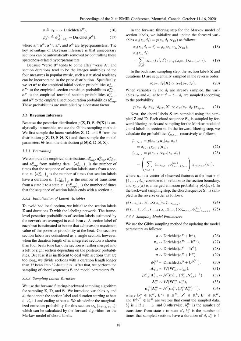
3.2 Model Formulation

As shown in Fig. 2, we formulate a hierarchical HSMMof observed features X with latent sequences of sectionlabels and abstract chord labels. Let S , S1:N be a se-quence of chord sequences, where Sn , sn,1:dn (sn,τ ∈{1, . . . ,M}) is a chord sequence in section n andM is themaximum number of chords in a section. The full proba-bilistic model p(X,Z,D,S) is defined as

p(X,Z,D,S) = p(X|Z,D,S)p(S|Z,D)p(Z,D), (1)

where p(X|Z,D,S) is an acoustic model of observed fea-tures X, p(S|Z,D) is a left-to-right Markov model of chord

Proceedings of the 21st ISMIR Conference, Montreal, Canada, October 11-16, 2020

16

labels S and p(Z,D) is an ergodic semi-Markov model ofsection labels Z with durations D.

3.2.1 Semi-Markov Chain of Section Labels

The ergodic semi-Markov model p(Z,D) in Eq. (1) repre-sents the generative process of section labels Z and theirdurations D as follows:

p(Z,D) = p(z1, d1)N∏n=2

p(zn, dn|zn−1, dn−1), (2)

where the individual terms are given by

p(z1, d1) = ρz1ψd1 , (3)

p(zn, dn|zn−1, dn−1) = πzn−1znψdn , (4)

p(zN , dN |zN−1, dN−1) = πzN−1zNψdNυzN , (5)

where ρz , πzz′ , and υz are the initial, transition, and ter-minal probabilities of section labels and ψd is the durationprobability.

3.2.2 Left-to-Right Markov Chain of Chord Labels

The left-to-right Markov model p(S|Z,D) in Eq. (1) rep-resents the generative process of chord labels S as follows:

p(S|Z,D) =N∏n=1

p(sn,1)

dn∏τ=2

p(sn,τ |sn,τ−1, zn), (6)

where the individual terms are given by

p(sn,1 = 1) = 1, (7)

p(sn,τ |sn,τ−1, zn) = φ(zn)sn,τ−1sn,τ , (8)

where zn is the corresponding section label and φ(z)ss′ is thetransition probability from state s to state s′. The left-to-right Markov model meets a condition that the initial statehas sn,1 = 1 and sn,τ1 ≤ sn,τ2 for τ1 < τ2. We introducea hyperparameter σ that describes the maximum number ofstates that may be skipped in a transition; a transition fromstate s to state s + σ is allowed. In this way, the modelallows chord labels to be repeated with some variations insections of the same label.

3.2.3 Emission of Acoustic Features

Given that the chroma features Xc, the MFCCs Xm, andthe mel spectra Xs are conditionally and temporally in-dependent, the acoustic model p(X|Z,D,S) in Eq. (1) isfactorized as follows:

p(X|Z,D,S) =T∏t=1

χczt,st(xct)χ

mzt(x

mt )χszt(x

st ), (9)

where zt and st are the section and chord labels at beatt, respectively, determined by the section-level latent vari-ables Z, D, and S, and χcz,s, χ

mz , and χsz are the emission

probabilities of chroma features xc, MFCCs xm, and melspectra xs, respectively.

The chroma features xc ∈ R12 are generated dependingon both the section label z and the chord label s havingthe left-to-right property. The chord/chroma repetitivenessis thus represented by applying the same set of emissionprobabilities to all sections of the same label. The emission

Observations

Latent states

section

chord

duration

chromafeatures

MFCCs

𝒁

𝑺

𝑫

𝑿!

𝑿"

8 bars 8 bars4 bars

A AB

1 1 2 2 3 3 1 1 2 2 1 1 1 2 2 3

mel spectra 𝑿#

Figure 2. Proposed LSTM-HSMM hybrid model.

probability χcz,s(xc) in Eq. (9) is given by a multivariate

Gaussian distribution as follows:

χcz,s(xc) = N (xc|µcz,s, (Λc

z,s)−1), (10)

where µcz,s and Λcz,s are a mean vector and a precision

matrix, respectively.The MFCCs xm ∈ R12 are generated depending on the

section label z. This allows the model to capture the homo-geneity of the timbral characteristics of each section. Theemission probability χmz (xm) in Eq. (9) is also given by amultivariate Gaussian distribution as follows:

χmz (xm) = N (xm|µmz , (Λmz )−1), (11)

where µmz and Λmz are a mean vector and a precision ma-

trix, respectively.The mel spectra xs ∈ R128 are generated depending

on the section label z. The emission probability χsz(xs) in

Eq. (9) is computed as follows:

χsz(xs) = p(xs|z) ∝ p(z|xs)

p(z), (12)

where p(z) is a unigram probability of section labels, andthe probability p(z|xs) is estimated by a labeling network(BLSTM) that infers section labels from mel spectra at theframe level. Let p(z|xs) be the average of the frame-leveloutputs of the network in beat units.

3.2.4 Prior Distributions Based on Musical Knowledge

To use prior knowledge about musical sections, we formu-late a Bayesian HSMM by putting conjugate prior distribu-tions on the model parameters Θ , {ρ,ψ,π,υ,φ,µ,Λ}[26]. We put Gaussian-Wishart prior distributions on themultivariate Gaussian parameters as follows:

µcz,s,Λcz,s ∼ N (µcz,s|mc

0, (βc0Λ

cz,s)−1)W(Λc

z,s|Wc0, ν

c0),

µmz ,Λmz ∼ N (µmz |mm

0 , (βm0 Λm

z )−1)W(Λmz |Wm

0 , νm0 ),

where mc0, βc0, Wc

0, νc0, mm0 , βm0 , Wm

0 , and νm0 are hy-perparameters. We then put Dirichlet prior distributions onthe categorical parameters as follows:

ρ , ρ1:K ∼ Dirichlet(aρ), (13)

ψ , ψ1:L ∼ Dirichlet(aψ), (14)

πz , πz(1:K) ∼ Dirichlet(aπz ), (15)


17

υ , υ1:K ∼ Dirichlet(aυ), (16)

φ(z)s , φ

(z)s(1:M) ∼ Dirichlet(aφ), (17)

where aρ, aψ , aπz , aυ , and aφ are hyperparameters. Thekey advantage of Bayesian inference is that unnecessarysections can be automatically removed by controlling thesesparseness-related hyperparameters.

Because “verse B” tends to come after “verse A”, andsection durations tend to be the integer multiples of thefour measures in popular music, such a statistical tendencycan be incorporated in the prior distribution. Specifically,we set aρ to the empirical initial section probabilities aρemp,aπz to the empirical section transition probabilities aπzemp,aυ to the empirical terminal section probabilities aυemp,and aψ to the empirical section duration probabilities aψemp.These probabilities are multiplied by a constant factor.

3.3 Bayesian Inference

Because the posterior distribution p(Z,D,S,Θ|X) is an-alytically intractable, we use the Gibbs sampling method.We first sample the latent variables Z, D, and S from thedistribution p(Z,D,S|Θ,X) and then sample the modelparameters Θ from the distribution p(Θ|Z,D,S,X).

3.3.1 Pretraining

We compute the empirical distributions aρemp, aψemp, aπzemp,and aυemp from training data.

(aρemp

)z

is the number oftimes that the sequence of section labels starts from a sec-tion z.

(aψemp

)d

is the number of times that section labelshave a duration d.

(aπzemp

)z′

is the number of transitionsfrom a state z to a state z′.

(aυemp

)z

is the number of timesthat the sequence of section labels ends with a section z.

3.3.2 Initialization of Latent Variables

To avoid bad local optima, we initialize the section labelsZ and durations D with the labeling network. The frame-level posterior probabilities of section labels estimated bythe network are averaged in each beat t. A section label ofeach beat is estimated to be one that achieves the maximumvalue of the posterior probability at the beat. Consecutivesection labels are considered as a single section; however,when the duration length of an integrated section is shorterthan four beats (one bar), the section is further merged intoa left or right section depending on the posterior probabil-ities. Because it is inefficient to deal with sections that aretoo long, we divide sections with a duration length longerthan 32 beats into 32-beat units. After that, we perform thesampling of chord sequences S and model parameters Θ.

3.3.3 Sampling Latent Variables

We use the forward filtering-backward sampling algorithmfor sampling Z, D, and S. We introduce variables zt anddt that denote the section label and duration starting at beatt−dt+1 and ending at beat t. We also define the marginal-ized emission probability for this section ωzt(xt−dt+1:t),which can be calculated by the forward algorithm for theMarkov model of chord labels.

In the forward filtering step for the Markov model ofsection labels, we initialize and update the forward vari-ables αt(zt, dt) = p(zt, dt,x1:t) as follows:

αt(zt, dt = t) = ρztψdtωzt(x1:t), (18)

αt(zt, dt)

=∑z′,d′

αt−dt(z′, d′)πz′ztψdtωzt(xt−dt+1:t). (19)

In the backward sampling step, the section labels Z anddurations D are sequentially sampled in the reverse order:

p(zT , dT |X) ∝ αT (zT , dT ). (20)

When variables zt and dt are already sampled, the vari-ables zt′ and dt′ at beat t′ = t− dt are sampled accordingto the probability

p(zt′ , dt′ |zt:T , dt:T ,X) ∝ αt′(zt′ , dt′)πzt′zt . (21)

Next, the chord labels S are sampled using the sam-pled Z and D. Each chord sequence Sn is sampled by for-ward filtering-backward sampling for the Markov model ofchord labels in section n. In the forward filtering step, wecalculate the probabilities ζn,sn,τ recursively as follows:

ζn,sn,1 = p(sn,1,x1|zn, dn)= δsn,11χzn,1(x1), (22)

ζn,sn,τ = p(sn,τ ,x1:τ |zn, dn) (23)

=

∑sn,τ−1

ζn,sn,τ−1φ(zn)sn,τ−1sn,τ

χzn,sn,τ (xτ ),

where xτ is a vector of observed features at the beat τ ∈{1, . . . , dn} considered in relation to the section boundary,and χz,s(x) is a merged emission probability p(x|z, s). Inthe backward sampling step, the chord sequence Sn is sam-pled in the reverse order as follows:

p(sn,dn |zn, dn,x1:dn)∝ζn,sn,dn , (24)

p(sn,τ |zn, dn, sn,τ+1:dn ,x1:dn)∝ζn,sn,τφ(zn)sn,τsn,τ+1. (25)

3.3.4 Sampling Model Parameters

We use the Gibbs sampling method for updating the modelparameters as follows:

ρ ∼ Dirichlet(aρ + bρ), (26)

πz ∼ Dirichlet(aπz + bπz ), (27)

ψ ∼ Dirichlet(aψ + bψ), (28)

υ ∼ Dirichlet(aυ + bυ), (29)

φ(z)s ∼ Dirichlet(aφ + bφ

(z)s ), (30)

Λcz,s ∼ W(Wc

z,s, νcz,s), (31)

µcz,s|Λcz,s ∼ N (mc

z,s, (βcz,sΛ

cz,s)−1), (32)

Λmz ∼ W(Wm

z , νmz ), (33)

µmz |Λmz ∼ N (mm

z , (βmz Λm

z )−1), (34)

where bρ ∈ RK , bπz ∈ RK , bψ ∈ RL, bυ ∈ RK ,and bφ

(z)s ∈ RM are vectors that count the sampled data.

bρz is 1 if z = z1 and 0 otherwise, bπzz′ is the number oftransitions from state z to state z′, bψd is the number oftimes that sampled sections have a duration of d, bυz is 1


18

if z = zN and 0 otherwise, and bφ(z)s

s′ is the number oftransitions from state s to state s′ in the Markov modelof chord labels in section z. The parameters mc

z,s, βcz,s,

Wcz,s, and νcz,s are calculated as follows:

βcz,s = βc0 +Nz,s, νcz,s = νc0 +Nz,s, (35)

mcz,s =

1

βcz,s(βc0m

c0 +Nz,sx

cz,s), (36)

(Wcz,s)−1 = (Wc

0)−1 +Nz,sU

cz,s

+βc0Nz,sβc0 +Nz,s

(xcz,s −mc0)(x

cz,s −mc

0)T, (37)

where we have defined

Nz,s =T∑t=1

δztzδsts, (38)

xcz,s =1

Nz,s

T∑t=1

δztzδstsxct , (39)

Ucz,s =

1

Nz,s

T∑t=1

δztzδsts(xct − xcz,s)(x

ct − xcz,s)

T. (40)

The parameters mmz , βmz , Wm

z , and νmz can be calculatedsimilarly.

3.3.5 Viterbi Training

Since the samples from the Gibbs sampler are not neces-sarily local optima of the posterior distribution, we applyViterbi training in the last step of the parameter estima-tion. Specifically, we apply the Viterbi algorithm (insteadof the forward filtering-backward sampling algorithm) toestimate the latent variables and update the model parame-ters to the expectation values of the posterior probabilities(instead of samples from those probabilities). It is knownthat Viterbi training is generally efficient for finding an ap-proximate local minimum [29].

3.3.6 Refinements

We introduce a weighting factor wdur(≥ 1) for the du-ration probability to enhance its effect. Specifically, wereplace the probability factor ψd in the forward algorithm(18) and (19) with (ψd)

wdur . Similar replacements are ap-plied to the Viterbi training step and the final estimationstep of the latent states explained in Section 3.4. We alsointroduce a weighting factor wlabel that balances the emis-sion probabilities for mel spectra with the other emissionprobabilities. We replace the emission probability χsz(x

s)in (9) with (χsz(x

s))wlabel .

3.4 Estimation of Musical Sections

After training the model parameters Θ, we compute themaximum a posteriori (MAP) estimate of the musical sec-tions. Specifically, we maximize the posterior probabilityp(Z,D|Θ,X) with respect to the section labels Z and du-rations D. This can be solved by integrating out the chordlabels S and applying the Viterbi algorithm for HSMMs[30] to the Markov model of section labels.

4. EVALUATION

Experiments were conducted to investigate the performanceof the proposed method.

4.1 Experimental Conditions

To evaluate our model, we used the 100 pieces from theRWC Popular Music Database [31] with structure anno-tations [32] for evaluation. We extracted chroma featuresusing the deep feature extractor [33] and MFCCs and melspectrograms using the librosa library [34]. Beat informa-tion was obtained using the madmom library [28]. Thelabeling network consisted of a single-layer BLSTM with2048 × 2 cells and a fully-connected layer with output di-mension K. The network was trained with 10-fold crossvalidation, and the empirical distributions aρemp, aψemp, aπzemp,and aυemp were trained with piece-wise cross validation forthe 100 pieces. For parameter estimation, we iterated theGibbs sampling 15 times and the Viterbi training 3 times,which took around five times longer than the duration ofan input signal with a standard CPU.

The hyperparameters of the proposed model were set asfollows: K = 10, L = 40, M = 16, σ = 1, wdur = 4,wlabel = 0.5, aρ = 1·aρemp, aπ = 1·aπemp, aψ = 64·aψemp,aυ = 1 · aυemp, aφ = I, mc

0 = E[Xc], βc0 = 64, Wc0 =

(νc0 cov[Xc])−1 with νc0 = 512, mm

0 = E[Xm], βm0 = 2,and Wm

0 = (νm0 cov[Xm])−1 with νm0 = 16, where I de-notes a vector with all entries equal to 1. The first param-eter K was determined according to the number of labelsused in [24], as shown in the legend in Fig. 3. The nexttwo parameters L and M were determined by consultingthe statistics of the annotated data. In the data, most sec-tions have a length of 40 beats or less. If we assume asection length of 32 beats (8 measures) and a chord dura-tion of 2 beats, the expected number of chords in each sec-tion is 16. The value of σ was set to 1 for simplicity. Theother parameters were determined by a coarse optimiza-tion w.r.t. the evaluation measures explained below. Eachparameter was optimized by a grid search, fixing the otherparameters. Further optimization of the parameters is leftfor future work.

We evaluated the estimation results in terms of segmen-tation, clustering, and labeling. The qualities of segmen-tation and clustering were evaluated in the same way asMIREX [35]. The quality of segmentation was evaluatedby the F-measures of section boundaries denoted by F0.5

and F3.0 [36]. Specifically, an estimated boundary is ac-cepted as correct if it is within ±0.5/3.0 seconds from theground-truth boundary. The precision rate is the percent-age of correct boundaries in estimated boundaries, the re-call rate is the percentage of true boundaries that are cor-rectly estimated, and the F-measures F0.5 and F3.0 are de-fined as the harmonic means of the precision and recallrates.

The quality of clustering was evaluated by the pairwiseF-measure denoted by Fpair [37] defined as follows. Wecompared pairs of frames (with a length of 100 ms) thatare labeled with the same class in an estimation result withthose in the ground truth. The precision rate, recall rate,


19

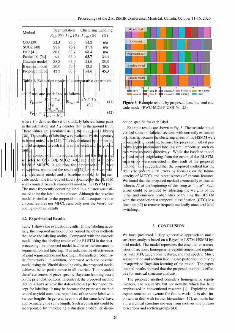
MethodSegmentation Clustering Labeling

F0.5 (%) F3.0 (%) Fpair (%) (%)

GS3 [39] 52.3 73.5 54.2 n/aSUG2 [40] 25.8 73.7 37.3 n/aFK2 [41] 30.0 65.7 63.4 n/aPaulus’09 [24] n/a 63.0 63.7 34.4Cascade model 38.3 63.9 54.9 38.8Baseline model 30.6 53.5 43.3 39.5Proposed model 43.3 66.5 54.6 45.3

Table 1. Evaluation results of a comparative experiment.

and F-measure are defined as follows:

Ppair =|PE ∩ PA||PE |

, Rpair =|PE ∩ PA||PA|

, (41)

Fpair =2PpairRpair

Ppair +Rpair, (42)

where PE denotes the set of similarly labeled frame pairsin the estimation and PA denotes that in the ground truth.These values are calculated using the mir_eval library[38]. The quality of labeling was evaluated by the accuracyin frame units, as in [24]. This is calculated by comparinga label assigned to each frame in the result and the groundtruth.

For comparison in the segmentation and the clustering,we refer to GS3 [39], SUG2 [40], and FK2 [41], pub-lished in MIREX. In addition, for comparison in all threeviewpoints, we quoted the result of [24] and ran two mod-els, a cascade model and a baseline model. In the cas-cade model, the frame-level labels obtained by the BLSTMwere counted for each cluster obtained by the HSMM [26].The most frequently occurring label in a cluster was esti-mated to be the label in that cluster. Although the baselinemodel is similar to the proposed model, it outputs neitherchroma features nor MFCCs and only uses the Viterbi de-coding to obtain results.

4.2 Experimental Results

Table 1 shows the evaluation results. In the labeling accu-racy, the proposed method outperformed the other methodsthat have the labeling ability. Compared with the cascademodel using the labeling results of the BLSTM in the post-processing, the proposed model had better performance insegmentation and labeling. This indicates the effectivenessof joint segmentation and labeling in the unified probabilis-tic framework. In addition, compared with the baselinemodel using the Viterbi decoding only, the proposed modelachieved better performance in all metrics. This revealedthe effectiveness of piece-specific Bayesian learning basedon the prior distributions. In contrast, the proposed methoddid not always achieve the state-of-the-art performance ex-cept for labeling. It may be because the proposed methodtended to yield unnatural repetitions of the same label withvarious lengths. In general, sections of the same label haveapproximately the same length. Such a constraint could beincorporated by introducing a duration probability distri-

0 sec 50 100 150 200 250introverse A

verse Bverse C

chorus Achorus B

bridge Aending

pre-chorusmisc

Ground truth

RNN result

Proposed model

Baseline model

Cascade model

Figure 3. Example results by proposed, baseline, and cas-cade model (RWC-MDB-P-2001 No. 25)

bution specific for each label.Example results are shown in Fig. 3. The cascade model

yielded some mislabeled sections with correctly estimatedboundaries because the clustering errors of the HSMM werepropagated. In contrast, because the proposed method per-forms segmentation and labeling simultaneously, such er-rors were reduced effectively. While the baseline modelyielded errors originating from the errors of the BLSTM,such errors were corrected in the result of the proposedmethod. This suggested that the proposed method has theability to prevent such errors by focusing on the homo-geneity of MFCCs and repetitiveness of chroma features.We found that the proposed method erroneously estimated“chorus A” at the beginning of this song as “intro”. Sucherrors could be avoided by adjusting the weights of theinitial and emission probabilities or training the BLSTMwith the connectionist temporal classification (CTC) lossfunction [42] to remove frequent musically unnatural labelswitching.

5. CONCLUSION

We have presented a deep generative approach to musicstructure analysis based on a Bayesian LSTM-HSMM hy-brid model. The model represents the essential character-istics of sections, homogeneity, repetitiveness, and regular-ity, with MFCCs, chroma features, and mel spectra. Musicsegmentation and section labeling are performed jointly byunsupervised Bayesian learning of the model. The exper-imental results showed that the proposed method is effec-tive for musical structure analysis.

The proposed method considers homogeneity, repeti-tiveness, and regularity, but not novelty, which has beenemphasized in conventional research [1]. Exploiting thisaspect remains an avenue for future work. It is also im-portant to deal with further hierarchies [17], as music hasa hierarchical structure moving from motives and phrasesto sections and section groups [43].


20

6. ACKNOWLEDGEMENTS

This work is supported in part by JST ACCEL No. JPM-JAC1602 and JSPS KAKENHI Nos. 16H01744, 19K20340,and 19H04137.

7. REFERENCES

[1] J. Paulus, M. Müller, and A. Klapuri, “State of the artreport: Audio-based music structure analysis,” in Inter-national Society for Music Information Retrieval Con-ference (ISMIR), 2010, pp. 625–636.

[2] J. Foote, “Automatic audio segmentation using a mea-sure of audio novelty,” in IEEE International Confer-ence on Multimedia and Expo (ICME), 2000, pp. 452–455.

[3] K. Jensen, “Multiple scale music segmentation usingrhythm, timbre, and harmony,” EURASIP Journal onApplied Signal Processing, vol. 2007, no. 1, pp. 159–159, 2007.

[4] M. Goto, “A chorus section detection method for mu-sical audio signals and its application to a music lis-tening station,” IEEE Transactions on Audio, Speech,and Language Processing (TASLP), vol. 14, no. 5, pp.1783–1794, 2006.

[5] J. Serrà, M. Müller, P. Grosche, and J. Arcos, “Unsu-pervised detection of music boundaries by time seriesstructure features,” in International Society for MusicInformation Retrieval Conference (ISMIR), 2012, pp.1613–1619.

[6] G. Peeters and V. Bisot, “Improving music structuresegmentation using lag-priors,” in International Soci-ety for Music Information Retrieval Conference (IS-MIR), 2014, pp. 337–342.

[7] J. Serrà, M. Müller, P. Grosche, and J. Arcos, “Un-supervised music structure annotation by time seriesstructure features and segment similarity,” IEEE Trans-actions on Multimedia, vol. 16, no. 5, pp. 1229–1240,2014.

[8] K. Ullrich, J. Schlüter, and T. Grill, “Boundary de-tection in music structure analysis using convolutionalneural networks,” in International Society for MusicInformation Retrieval Conference (ISMIR), 2014, pp.417–422.

[9] T. Grill and J. Schlüter, “Music boundary detection us-ing neural networks on combined features and two-level annotations,” in International Society for MusicInformation Retrieval Conference (ISMIR), 2015, pp.531–537.

[10] J. B. L. Smith and M. Goto, “Using priors to improveestimates of music structure,” in International Societyfor Music Information Retrieval Conference (ISMIR),2016, pp. 554–560.

[11] G. Sargent, F. Bimbot, and E. Vincent, “Estimating thestructural segmentation of popular music pieces underregularity constraints,” IEEE Transactions on Audio,Speech and Language Processing (TASLP), vol. 25,no. 2, pp. 344–358, 2017.

[12] A. Maezawa, “Music boundary detection based on ahybrid deep model of novelty, homogeneity, repeti-tion and duration,” in IEEE International Conferenceon Acoustics, Speech and Signal Processing (ICASSP),2019, pp. 206–210.

[13] M. Cooper and J. Foote, “Summarizing popular mu-sic via structural similarity analysis,” in IEEE Work-shop on Applications of Signal Processing to Audioand Acoustics (WASPAA), 2003, pp. 127–130.

[14] M. M. Goodwin and J. Laroche, “A dynamicprogramming approach to audio segmentation andspeech/music discrimination,” in IEEE InternationalConference on Acoustics, Speech, and Signal Process-ing (ICASSP), 2004, pp. 309–312.

[15] H. Grohganz, M. Clausen, N. Jiang, and M. Müller,“Converting path structures into block structures us-ing eigenvalue decompositions of self-similarity ma-trices,” in International Society for Music InformationRetrieval Conference (ISMIR), 2013, pp. 209–214.

[16] O. Nieto and T. Jehan, “Convex non-negative matrixfactorization for automatic music structure identifica-tion,” in IEEE International Conference on Acoustics,Speech and Signal Processing (ICASSP), 2013, pp.236–240.

[17] B. McFee and D. P. W. Ellis, “Analyzing song struc-ture with spectral clustering,” in International Societyfor Music Information Retrieval Conference (ISMIR),2014, pp. 405–410.

[18] T. Cheng, J. B. L. Smith, and M. Goto, “Music struc-ture boundary detection and labelling by a deconvolu-tion of path-enhanced self-similarity matrix,” in Inter-national Society for Music Information Retrieval Con-ference (ISMIR), 2018, pp. 106–110.

[19] J.-J. Aucouturier and M. Sandler, “Segmentation ofmusical signals using hidden Markov models,” in Au-dio Engineering Society (AES) Convention, 2001, pp.1–8.

[20] M. Levy and M. Sandler, “New methods in structuralsegmentation of musical audio,” in European SignalProcessing Conference (EUSIPCO), 2006, pp. 1–5.

[21] L. Ren, D. Dunson, S. Lindroth, and L. Carin, “Dy-namic nonparametric Bayesian models for analysis ofmusic,” Journal of the American Statistical Association(JASA), vol. 105, no. 490, pp. 458–472, 2008.

[22] L. Barrington, A. B. Chan, and G. Lanckriet, “Mod-eling music as a dynamic texture,” IEEE Transactionson Audio, Speech and Language Processing (TASLP),vol. 18, no. 3, pp. 602–612, 2010.


21

[23] F. Kaiser and G. Peeters, “A simple fusion method ofstate and sequence segmentation for music structurediscovery,” in International Society for Music Informa-tion Retrieval Conference (ISMIR), 2013, pp. 257–262.

[24] J. Paulus and A. Klapuri, “Music structure analysis us-ing a probabilistic fitness measure and a greedy searchalgorithm,” IEEE Transactions on Audio, Speech andLanguage Processing (TASLP), vol. 17, no. 6, pp.1159–1170, 2009.

[25] ——, “Labelling the structural parts of a music piecewith markov models,” in Computer Music Modelingand Retrieval (CMMR), 2008, pp. 166–176.

[26] G. Shibata, R. Nishikimi, E. Nakamura, and K. Yoshii,“Statistical music structure analysis based on ahomogeneity-, repetitiveness-, and regularity-aware hi-erarchical hidden semi-markov model,” in Interna-tional Society for Music Information Retrieval Confer-ence (ISMIR), 2019, pp. 268–275.

[27] N. C. Maddage, C. Xu, M. S. Kankanhalli, andX. Shao, “Content-based music structure analysiswith applications to music semantics understand-ing,” in ACM International Conference on Multimedia(ACMMM), 2004, pp. 112–119.

[28] S. Böck, F. Korzeniowski, J. Schlüter, F. Krebs, andG. Widmer, “madmom: A new python audio and musicsignal processing library,” in ACM International Con-ference on Multimedia (ACMMM), 2016, pp. 1174–1178.

[29] A. Allahverdyan and A. Galstyan, “Comparative anal-ysis of Viterbi training and maximum likelihood esti-mation for HMMs,” in Advances in Neural InformationProcessing Systems (NIPS), 2011, pp. 1674–1682.

[30] S.-Z. Yu, “Hidden semi-Markov models,” Artificial In-telligence, vol. 174, no. 2, pp. 215–243, 2010.

[31] M. Goto, H. Hashiguchi, T. Nishimura, and R. Oka,“RWC music database: Popular, classical and jazz mu-sic databases,” in International Conference on MusicInformation Retrieval (ISMIR), 2002, pp. 287–288.

[32] M. Goto, “AIST annotation for the RWC musicdatabase,” in International Conference on Music Infor-mation Retrieval (ISMIR), 2006, pp. 359–360.

[33] Y. Wu and W. Li, “Automatic audio chord recogni-tion with MIDI-trained deep feature and BLSTM-CRFsequence decoding model,” IEEE/ACM Transactionson Audio, Speech and Language Processing (TASLP),vol. 27, no. 2, pp. 355–366, 2019.

[34] B. McFee, C. Raffel, D. Liang, D. P. W. Ellis,M. McVicar, E. Battenberg, and O. Nieto, “librosa:Audio and music signal analysis in python,” in Pythonin Science Conference, 2015, pp. 18–24.

[35] A. F. Ehmann, M. Bay, J. S. Downie, I. Fujinaga, andD. D. Roure, “Music structure segmentation algorithmevaluation: Expanding on MIREX 2010 analyses anddatasets,” in International Society for Music Informa-tion Retrieval Conference (ISMIR), 2011, pp. 561–566.

[36] D. Turnbull, G. Lanckriet, E. Pampalk, and M. Goto,“A supervised approach for detecting boundaries inmusic using difference features and boosting,” in Inter-national Conference on Music Information Retrieval(ISMIR), 2007, pp. 51–54.

[37] M. Levy and M. Sandler, “Structural segmentation ofmusical audio by constrained clustering,” IEEE Trans-actions on Audio, Speech, and Language Processing(TASLP), vol. 16, no. 2, pp. 318–326, 2008.

[38] C. Raffel, B. McFee, E. J. Humphrey, J. Salamon,O. Nieto, D. Liang, and D. P. W. Ellis, “mir_eval:A transparent implementation of common MIR met-rics,” in International Society for Music InformationRetrieval Conference (ISMIR), 2014.

[39] T. Grill and J. Schlüter, “Structural segmentationwith convolutional neural networks mirex submission,”in Music Information Retrieval Evaluation eXchange(MIREX), 2015.

[40] J. Schlüter, K. Ullrich, and T. Grill, “Structural seg-mentation with convolutional neural networks mirexsubmission,” in Music Information Retrieval Evalua-tion eXchange (MIREX), 2014.

[41] F. Kaiser and G. Peeters, “Music structural segmen-tation task: Ircamstructure submission,” in Music In-formation Retrieval Evaluation eXchange (MIREX),2013.

[42] A. Graves, S. Fernández, F. Gomez, and J. Schmid-huber, “Connectionist temporal classification: la-belling unsegmented sequence data with recurrent neu-ral networks,” in International Conference on MachineLearning (ICML), 2006, pp. 369–376.

[43] F. Lerdahl and R. Jackendoff, A Generative Theory ofTonal Music. MIT Press, 1983.


22

Documents

MUSIC STRUCTURE ANALYSIS BASED ON AN LSTM-HSMM …