Muscle–tendon mechanics explain unexpected effects of

RESEARCH ARTICLE

Muscle–tendon mechanics explain unexpected effects ofexoskeleton assistance on metabolic rate during walkingRachel W. Jackson1,*, Christopher L. Dembia2, Scott L. Delp2,3 and Steven H. Collins1,4

ABSTRACTThe goal of this study was to gain insight into how ankle exoskeletonsaffect the behavior of the plantarflexor muscles during walking. Usingdata from previous experiments, we performed electromyography-driven simulations of musculoskeletal dynamics to explore howchanges in exoskeleton assistance affected plantarflexor muscle–tendon mechanics, particularly for the soleus. We used a model ofmuscle energy consumption to estimate individual muscle metabolicrate. As average exoskeleton torque was increased, while no netexoskeleton work was provided, a reduction in tendon recoil led to anincrease in positive mechanical work performed by the soleusmusclefibers. As net exoskeleton work was increased, both soleus musclefiber force and positive mechanical work decreased. Trends in thesum of the metabolic rates of the simulated muscles correlatedwell with trends in experimentally observed whole-body metabolicrate (R2=0.9), providing confidence in our model estimates. Oursimulation results suggest that different exoskeleton behaviors canalter the functioning of themuscles and tendons acting at the assistedjoint. Furthermore, our results support the idea that the series tendonhelps reduce positive work done by the muscle fibers by storing andreturning energy elastically. We expect the results from this study topromote the use of electromyography-driven simulations to gaininsight into the operation of muscle–tendon units and to guide thedesign and control of assistive devices.

KEY WORDS: Biomechanics, Series elastic element, Ankle footorthosis, Gait, Musculoskeletal modelling

INTRODUCTIONThe plantarflexor muscle–tendon units seem tuned for near-optimalefficiency and power production during unassisted locomotion.During normal walking, the ankle plantarflexor muscles produceforce nearly isometrically throughout mid-stance, while the Achillestendon lengthens and stores mechanical energy (Fukunaga et al.,2001). This isometric muscle force production is economicalbecause muscles consume relatively little energy to produce force atconstant length (Biewener, 1998; Biewener and Roberts, 2000). Atthe end of stance, the plantarflexor muscles actively shorten andthe Achilles tendon simultaneously recoils (Fukunaga et al., 2001;Ishikawa et al., 2005; Rubenson et al., 2012), generating asignificant amount of positive power at push-off (Winter, 1990;

Meinders et al., 1998). Elastic energy storage and recovery in theAchilles tendon helps to reduce plantarflexor muscle work (Robertset al., 1997; Ishikawa et al., 2005). Furthermore, the stiffness ofthe Achilles tendon, in conjunction with the resting length of theplantarflexor muscle fibers, has been shown to maximizeplantarflexor muscle efficiency during walking and running byallowing the muscle fibers to operate at favorable lengths andvelocities during positive fiber work production (Roberts et al.,1997; Roberts, 2002; Lichtwark and Wilson, 2007; Taylor, 2007;Lichtwark and Wilson, 2008; Lichtwark and Barclay, 2010; Arnoldet al., 2013). Any change to the stiffness of the Achilles tendoncan affect the mechanics of the plantarflexor muscle fibers andconsequently alter muscle energy consumption (Lichtwark andWilson, 2007). The architecture of the plantarflexor muscles, thecompliance of the Achilles tendon, and the interaction betweenthese mechanisms enables economical operation.

The complexity of these plantarflexor muscle–tendon mechanicsposes a challenge for the design of exoskeletons intended to operatein concert with the musculoskeletal system. Previous experimentsand simulations of a musculoskeletal model have shown that elasticexoskeletons worn during bilateral hopping significantly reduceplantarflexor muscle force, but not muscle work (Farris andSawicki, 2012; Farris et al., 2013, 2014; Robertson et al., 2014).Although large reductions were observed in whole-body metabolicrate, estimated metabolic energy consumed by the plantarflexormuscles was not significantly reduced, likely due to unfavorablechanges in the operating lengths and velocities of the muscle fibers(Farris et al., 2014). Simulations of a simplified, lumped modelof the plantarflexor muscle–tendon units acting in parallel with apassive exoskeleton during walking, with fixed joint kinematics,similarly suggest a disruption to the normal operation of theplantarflexor muscle–tendon units (Sawicki and Khan, 2016). Wewere curious to see if similar mechanisms could explain the effect ofdifferent types of exoskeleton assistance on locomotor coordinationand metabolic rate that we observed in a prior study.

We previously conducted an experiment in which subjects walkedin eight conditions with different amounts of net work and averageplantarflexion torque provided by an exoskeleton worn on one ankle(Jackson and Collins, 2015). We expected that providing net positiveexoskeleton work at the ankle joint would replace or augment positivework performed by the plantarflexormuscles and reduce the associatedmetabolic cost (Donelan et al., 2002; Gordon et al., 2009). Weexpected that providing plantarflexion torque about the ankle joint,without providing any net work, would offload plantarflexor muscleforces and reduce the metabolic cost associated with force production(Grabowski et al., 2005). Providing increasing amounts of netexoskeleton work decreased metabolic rate as expected. In contrastwith our predictions, providing increasing amounts of averageexoskeleton torque increased metabolic rate. We thought thesesurprising results might be explained by changes in the dynamicinteractions between muscles and tendons at the assisted joint.Received 30 September 2016; Accepted 21 March 2017

1Department of Mechanical Engineering, Carnegie Mellon University, Pittsburgh,PA 15213, USA. 2Department of Mechanical Engineering, Stanford University,Stanford, CA 94305, USA. 3Department of Bioengineering, Stanford University,Stanford, CA 94305, USA. 4Robotics Institute, Carnegie Mellon University,Pittsburgh, PA 15213, USA.

*Author for correspondence ([email protected])

R.W.J., 0000-0002-0938-1300

2082

© 2017. Published by The Company of Biologists Ltd | Journal of Experimental Biology (2017) 220, 2082-2095 doi:10.1242/jeb.150011

Journal

ofEx

perim

entalB

iology

mailto:[email protected]

http://orcid.org/0000-0002-0938-1300

We were unable to explore changes at the muscle–tendon levelduring assisted walking using direct measurement in our previousstudy. Although muscle fiber length changes can be measured usingultrasound imaging, the number of muscles that can be imaged islimited. Furthermore, it is not yet feasible to directly measureindividual muscle force and metabolic rate during locomotortasks in humans. An alternative approach for investigating howplantarflexor muscle–tendon mechanics are affected by differentexoskeleton behaviors is to conduct simulations with amusculoskeletal model. Driving a musculoskeletal model withexperimentally measured electromyography and joint kinematics isone promising simulation technique for generating realisticestimates of muscle–tendon mechanics (Lloyd and Besier, 2003;Arnold et al., 2013; Farris et al., 2014; Markowitz and Herr, 2016).Simulated muscle–tendon mechanics can be fed into models ofmuscle energy consumption to obtain estimates of muscle-levelenergetics (Umberger et al., 2003; Bhargava et al., 2004; Umbergerand Rubenson, 2011; Uchida et al., 2016). Such estimates couldpotentially provide an explanation for the observed changes inwhole-body energy consumption.The purpose of this study was to explore how the mechanics and

energetics of the plantarflexor muscle–tendon units change whensubjected to different perturbations applied by an ankle exoskeleton.We used muscle activity and joint kinematics data to drivesimulations of a musculoskeletal model and obtain estimates ofmuscle-level mechanics and energetics. We focused ourmusculoskeletal analyses on the soleus because observed changeswere most pronounced in this muscle–tendon unit, and it is themuscle–tendon unit most analogous to the exoskeleton. Wehypothesized that providing exoskeleton torque without providingany net work detuned the soleus muscle–tendon unit, leading toreduced elastic recoil of the tendon and increased work by themuscle fibers. We hypothesized that providing net positiveexoskeleton work, focused at the end of stance, more fullyreplaced the role of the soleus muscle–tendon unit, therebyreducing energy consumed at the ankle joint and elsewhere. Weexpected the results from this study to shed light on howexoskeletons should interact with the muscles and tendons toachieve the greatest benefits.

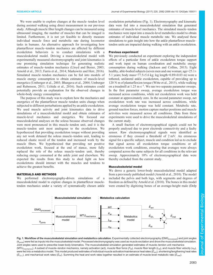
MATERIALS AND METHODSWe performed electromyography-driven simulations of amusculoskeletal model to explore changes in plantarflexor muscle-tendon mechanics under a variety of systematically chosen ankle

exoskeleton perturbations (Fig. 1). Electromyography and kinematicdata were fed into a musculoskeletal simulation that generatedestimates of muscle-level mechanics. The simulated muscle–tendonmechanics were input into a muscle-level metabolics model to obtainestimates of individual muscle metabolic rate. We analysed thesesimulations to gain insight into how the ankle plantarflexor muscle–tendon units are impacted during walking with an ankle exoskeleton.

Previous experimentWe previously conducted an experiment exploring the independenteffects of a particular form of ankle exoskeleton torque supportand work input on human coordination and metabolic energyconsumption during walking (Jackson and Collins, 2015). Eighthealthy, able-bodied subjects (sevenmen and onewoman; age=25.1±5.1 years; body mass=77.5±5.6 kg; leg length=0.89±0.03 m) wore atethered, unilateral ankle exoskeleton, capable of providing up to120 N m of plantarflexion torque (Witte et al., 2015), while walkingon a treadmill at 1.25 m s–1. We ran two separate parameter sweeps.In the first parameter sweep, average exoskeleton torque wasincreased across conditions, while net exoskeleton work was heldconstant at approximately zero. In the second parameter sweep, netexoskeleton work rate was increased across conditions, whileaverage exoskeleton torque was held constant. Metabolic rate,ground reaction forces, motion capture marker positions and muscleactivities were measured across all conditions. Data from theseexperiments were used to drive the musculoskeletal simulations ofthe current study.

A small fraction of electromyographical signals could not beproperly analysed due to poor electrode connectivity and a faultysensor. Raw electromyographical signals were identified aserroneous if they crossed a threshold of 2 mV. An erroneoussignal for a specific subject, muscle and condition led us to excludethat signal across all exoskeleton torque conditions or allexoskeleton work conditions, ensuring that averages were alwayscomputed across the same subjects for all conditions in the relevantsweep. Approximately 10% of electromyographical data werethereby excluded from the current study.

Musculoskeletal modelWe drove a generic lower-body musculoskeletal model adaptedfrom a previously published model (Arnold et al., 2010). The modelincluded the pelvis and both legs, with segments and degrees offreedom as defined by Arnold et al. (2010). The bones in this modelwere created by digitizing bones of an average-height male (Delp

EMGprocessed

Musculoskeletalmodel

vMEW

Emet.

act

FM

LM

Metabolicsmodel

.Eact

.ES/L

+

+

+

MTUmechanics

θjoints

Musculoskeletal simulation Metabolics calculation

.

Fig. 1. Workflow of the musculoskeletal simulation andmetabolics calculation. Experimentally collected electromyography (EMGprocessed) and joint angles(θjoints) were fed as inputs into themusculoskeletal model. Processed electromyography was used asmuscle excitation and drove themusculoskeletal simulation.Joint angles were used to prescribe lower-body kinematics. The musculoskeletal simulation generated estimates of muscle–tendon unit mechanics(MTUmechanics). A subset of muscle–tendon mechanics, namely activation (act), muscle fiber force (FM), muscle fiber length (LM), and muscle fiber velocity (vM),were fed into ametabolicsmodel. This model produced estimates of individual muscle activation/maintenance heat rates ( _Eact), shortening/lengthening heat rates( _ES=L), and mechanical work rates ( _EW). Summing the heat and work rates together resulted in an estimate of muscle-level metabolic rate ( _Emet).

2083

RESEARCH ARTICLE Journal of Experimental Biology (2017) 220, 2082-2095 doi:10.1242/jeb.150011

Journal

ofEx

perim

entalB

iology

et al., 1990; Arnold et al., 2010). We chose this model because it haspreviously been used to examine muscle fiber dynamics duringhuman walking and running at different speeds (Arnold et al., 2013)and to understand the effects of elastic ankle exoskeletons on themechanics and energetics of muscles during hopping (Farris et al.,2014).Of the original 35 lower-limb muscles in the model, we only

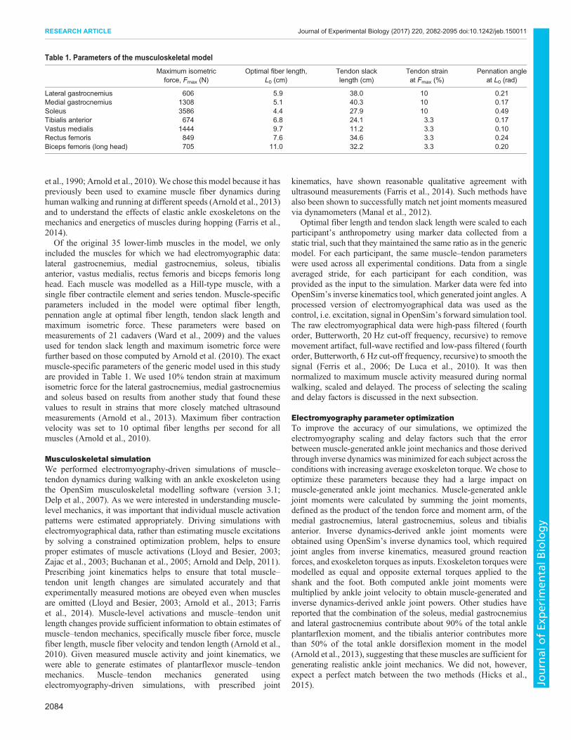
included the muscles for which we had electromyographic data:lateral gastrocnemius, medial gastrocnemius, soleus, tibialisanterior, vastus medialis, rectus femoris and biceps femoris longhead. Each muscle was modelled as a Hill-type muscle, with asingle fiber contractile element and series tendon. Muscle-specificparameters included in the model were optimal fiber length,pennation angle at optimal fiber length, tendon slack length andmaximum isometric force. These parameters were based onmeasurements of 21 cadavers (Ward et al., 2009) and the valuesused for tendon slack length and maximum isometric force werefurther based on those computed by Arnold et al. (2010). The exactmuscle-specific parameters of the generic model used in this studyare provided in Table 1. We used 10% tendon strain at maximumisometric force for the lateral gastrocnemius, medial gastrocnemiusand soleus based on results from another study that found thesevalues to result in strains that more closely matched ultrasoundmeasurements (Arnold et al., 2013). Maximum fiber contractionvelocity was set to 10 optimal fiber lengths per second for allmuscles (Arnold et al., 2010).

Musculoskeletal simulationWe performed electromyography-driven simulations of muscle–tendon dynamics during walking with an ankle exoskeleton usingthe OpenSim musculoskeletal modelling software (version 3.1;Delp et al., 2007). As we were interested in understanding muscle-level mechanics, it was important that individual muscle activationpatterns were estimated appropriately. Driving simulations withelectromyographical data, rather than estimating muscle excitationsby solving a constrained optimization problem, helps to ensureproper estimates of muscle activations (Lloyd and Besier, 2003;Zajac et al., 2003; Buchanan et al., 2005; Arnold and Delp, 2011).Prescribing joint kinematics helps to ensure that total muscle–tendon unit length changes are simulated accurately and thatexperimentally measured motions are obeyed even when musclesare omitted (Lloyd and Besier, 2003; Arnold et al., 2013; Farriset al., 2014). Muscle-level activations and muscle–tendon unitlength changes provide sufficient information to obtain estimates ofmuscle–tendon mechanics, specifically muscle fiber force, musclefiber length, muscle fiber velocity and tendon length (Arnold et al.,2010). Given measured muscle activity and joint kinematics, wewere able to generate estimates of plantarflexor muscle–tendonmechanics. Muscle–tendon mechanics generated usingelectromyography-driven simulations, with prescribed joint

kinematics, have shown reasonable qualitative agreement withultrasound measurements (Farris et al., 2014). Such methods havealso been shown to successfully match net joint moments measuredvia dynamometers (Manal et al., 2012).

Optimal fiber length and tendon slack length were scaled to eachparticipant’s anthropometry using marker data collected from astatic trial, such that they maintained the same ratio as in the genericmodel. For each participant, the same muscle–tendon parameterswere used across all experimental conditions. Data from a singleaveraged stride, for each participant for each condition, wasprovided as the input to the simulation. Marker data were fed intoOpenSim’s inverse kinematics tool, which generated joint angles. Aprocessed version of electromyographical data was used as thecontrol, i.e. excitation, signal in OpenSim’s forward simulation tool.The raw electromyographical data were high-pass filtered (fourthorder, Butterworth, 20 Hz cut-off frequency, recursive) to removemovement artifact, full-wave rectified and low-pass filtered (fourthorder, Butterworth, 6 Hz cut-off frequency, recursive) to smooth thesignal (Ferris et al., 2006; De Luca et al., 2010). It was thennormalized to maximum muscle activity measured during normalwalking, scaled and delayed. The process of selecting the scalingand delay factors is discussed in the next subsection.

Electromyography parameter optimizationTo improve the accuracy of our simulations, we optimized theelectromyography scaling and delay factors such that the errorbetween muscle-generated ankle joint mechanics and those derivedthrough inverse dynamics was minimized for each subject across theconditions with increasing average exoskeleton torque. We chose tooptimize these parameters because they had a large impact onmuscle-generated ankle joint mechanics. Muscle-generated anklejoint moments were calculated by summing the joint moments,defined as the product of the tendon force and moment arm, of themedial gastrocnemius, lateral gastrocnemius, soleus and tibialisanterior. Inverse dynamics-derived ankle joint moments wereobtained using OpenSim’s inverse dynamics tool, which requiredjoint angles from inverse kinematics, measured ground reactionforces, and exoskeleton torques as inputs. Exoskeleton torques weremodelled as equal and opposite external torques applied to theshank and the foot. Both computed ankle joint moments weremultiplied by ankle joint velocity to obtain muscle-generated andinverse dynamics-derived ankle joint powers. Other studies havereported that the combination of the soleus, medial gastrocnemiusand lateral gastrocnemius contribute about 90% of the total ankleplantarflexion moment, and the tibialis anterior contributes morethan 50% of the total ankle dorsiflexion moment in the model(Arnold et al., 2013), suggesting that these muscles are sufficient forgenerating realistic ankle joint mechanics. We did not, however,expect a perfect match between the two methods (Hicks et al.,2015).

Table 1. Parameters of the musculoskeletal model

Maximum isometricforce, Fmax (N)

Optimal fiber length,L0 (cm)

Tendon slacklength (cm)

Tendon strainat Fmax (%)

Pennation angleat L0 (rad)

Lateral gastrocnemius 606 5.9 38.0 10 0.21Medial gastrocnemius 1308 5.1 40.3 10 0.17Soleus 3586 4.4 27.9 10 0.49Tibialis anterior 674 6.8 24.1 3.3 0.17Vastus medialis 1444 9.7 11.2 3.3 0.10Rectus femoris 849 7.6 34.6 3.3 0.24Biceps femoris (long head) 705 11.0 32.2 3.3 0.20

2084


Journal

ofEx

perim

entalB

iology

To obtain the optimal values of the scaling and delay factors forthe muscles acting about the ankle joint, we performed gradientdescent optimization. In order to address differences across subjects,we used scaling and delay factors that were subject specific. For agiven subject, the same delay was used for all muscles, while adifferent scaling factor was used for each muscle. Peak muscleactivation during walking, relative to maximum voluntarycontraction of that muscle, varies significantly across muscles,therefore suggesting the importance of muscle-specific scalingfactors (Perry and Burnfield, 2010). Differences inelectromechanical delay across muscles is a more complicatedissue (Corcos et al., 1992; Hug et al., 2011). While studies haveshown that the delay may be muscle dependent (Conchola et al.,2013), we were able to achieve sufficiently accurate timing of jointmoments and powers without such added complexity. Furthermore,previous studies have used a single electromechanical delay acrossmuscles and subjects and obtained reasonable results (Lloyd andBesier, 2003; Arnold et al., 2013).In total, there were five optimization parameters for each subject:

the delay, the medial gastrocnemius scaling factor, the lateralgastrocnemius scaling factor, the soleus scaling factor, and thetibialis anterior scaling factor. The root mean square errors(RMSEs) between the muscle-generated ankle joint moments andpowers and the inverse dynamics-derived ankle joint moments andpowers were used to quantify the quality of fit. The norm of theRMSEs across the five increasing average exoskeleton torqueconditions was chosen as the objective function. The optimizedparameters for each subject are provided in Table 2. Because oursimulations only include three muscles that cross the knee and hipjoints, muscle-generated knee and hip joint mechanics should not beexpected to match inverse dynamics-derived knee and hip jointmechanics (Arnold et al., 2013). Therefore we did not optimize thescaling factors for these three muscles, but estimated them as thepercentage of the maximum voluntary contraction produced duringnormal walking observed in other experiments (Perry and Burnfield,2010).

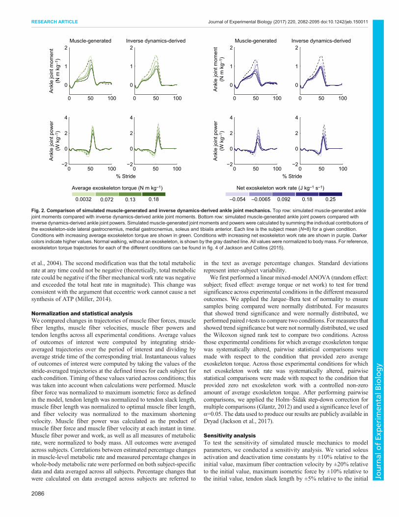
Optimization testingThe optimized parameters produced reasonable ankle jointmoments and powers (Fig. 2). The average RMSE, over subjectsand conditions, between muscle-generated and inverse dynamics-derived ankle joint moments was 0.13 N m kg–1, which was 11% ofthe average peak of the inverse dynamics-derived ankle jointmoment (1.2 N m kg–1). The average RMSE between muscle-generated and inverse dynamics-derived ankle joint powers was0.19 W kg–1, which was 9% of the average peak of the inversedynamics-derived ankle joint power (2.2 W kg–1). Muscle-generated ankle joint moments were found to be within twostandard deviations of inverse dynamics-derived ankle joint

moments, on average, which has been considered acceptable byother researchers (Hicks et al., 2015). The error in the timing of peaksubject-averaged joint moments and powers had a maximum valueof 1.6% of the gait cycle across all conditions. We were mostinterested in trends in ankle joint moments and powers withincreasing average exoskeleton torque and net exoskeleton work, soan exact match in the absolute values of muscle-generated andinverse dynamics-derived ankle joint mechanics was not necessary.

Metabolics modelWe used the results of the electromyography-driven simulations toestimate the energy consumed by each muscle using a modifiedversion of Umberger’s muscle metabolics model (Umberger et al.,2003; Umberger, 2010; Uchida et al., 2016). The metabolics modelcontains three different heat rates: the activation/maintenanceheat rate, the fiber shortening/lengthening heat rate, and the fibermechanical work rate. These heat rates depend in part on themuscle’s excitation, activation, fiber length, fiber velocity and fiberforce. We explored the effect of each heat rate on the total metabolicrate for the muscles under consideration. Additionally, we summedthe metabolic rates for each of the muscles simulated in our studyand investigated how well estimated trends in individual andsummed muscle metabolic rates explained changes in whole-bodymetabolic rate.

A lack of comparative experimental data makes it difficult tovalidate metabolics models. Other studies have validated theirmetabolics estimates by comparing simulated whole-bodymetabolic rate, defined as the sum of the individually simulatedmuscle metabolic rates, and indirect calorimetry (Umberger et al.,2003; Markowitz and Herr, 2016). As our study only includes asubset of potentially costly muscles, we did not expect the sum ofmetabolic rates of these muscles to accurately represent absolutechanges in whole-body metabolic rate. Furthermore, we were mostinterested in trends across the different experimental conditions, asopposed to absolute differences. For these reasons, we limit ourvalidation to the percentage change in the sum of the individuallysimulated muscle metabolic rates.

The version of Umberger’s metabolics model that is implementedin OpenSim is configurable, and we chose to use the originalversion of Umberger’s metabolics model (Umberger et al., 2003)with two modifications introduced by Uchida et al. (2016), as thesemodifications provided more accurate estimates compared withindirect calorimetry in similar studies. The first modification was theaddition of a model of orderly fiber recruitment. Umberger’s modelassumes that the ratio of slow- to fast-twitch fibers that are recruitedis equal to the ratio of slow- to fast-twitch fibers comprising themuscle. In the modified model, the ratio of slow- to fast-twitchfibers that are recruited instead varies with excitation so that fast-twitch fibers are increasingly used as excitation increases (Bhargava

Table 2. Optimized electromyography scaling factors and delays

Subject Delay (ms)Medial gastrocnemius

scaling factorLateral gastrocnemius

scaling factorSoleus scaling

factorTibialis anteriorscaling factor

1 0 0.10 0.45 0.95 0.312 0 0.23 0.37 0.94 0.553 0 0.26 0.26 0.90 0.444 0 0.26 0.26 0.90 0.445 5.8 0.12 0.10 0.86 0.466 0 0.31 0.30 0.95 0.447 0 0.29 0.42 0.95 0.398 7.8 0.12 0.10 0.95 0.49

2085


Journal

ofEx

perim

entalB

iology

et al., 2004). The second modification was that the total metabolicrate at any time could not be negative (theoretically, total metabolicrate could be negative if the fiber mechanical work rate was negativeand exceeded the total heat rate in magnitude). This change wasconsistent with the argument that eccentric work cannot cause a netsynthesis of ATP (Miller, 2014).

Normalization and statistical analysisWe compared changes in trajectories of muscle fiber forces, musclefiber lengths, muscle fiber velocities, muscle fiber powers andtendon lengths across all experimental conditions. Average valuesof outcomes of interest were computed by integrating stride-averaged trajectories over the period of interest and dividing byaverage stride time of the corresponding trial. Instantaneous valuesof outcomes of interest were computed by taking the values of thestride-averaged trajectories at the defined times for each subject foreach condition. Timing of these values varied across conditions; thiswas taken into account when calculations were performed. Musclefiber force was normalized to maximum isometric force as definedin the model, tendon length was normalized to tendon slack length,muscle fiber length was normalized to optimal muscle fiber length,and fiber velocity was normalized to the maximum shorteningvelocity. Muscle fiber power was calculated as the product ofmuscle fiber force and muscle fiber velocity at each instant in time.Muscle fiber power and work, as well as all measures of metabolicrate, were normalized to body mass. All outcomes were averagedacross subjects. Correlations between estimated percentage changesin muscle-level metabolic rate and measured percentage changes inwhole-body metabolic rate were performed on both subject-specificdata and data averaged across all subjects. Percentage changes thatwere calculated on data averaged across subjects are referred to

in the text as average percentage changes. Standard deviationsrepresent inter-subject variability.

We first performed a linear mixed-model ANOVA (random effect:subject; fixed effect: average torque or net work) to test for trendsignificance across experimental conditions in the different measuredoutcomes. We applied the Jarque–Bera test of normality to ensuresamples being compared were normally distributed. For measuresthat showed trend significance and were normally distributed, weperformed paired t-tests to compare two conditions. Formeasures thatshowed trend significance but were not normally distributed, we usedthe Wilcoxon signed rank test to compare two conditions. Acrossthose experimental conditions for which average exoskeleton torquewas systematically altered, pairwise statistical comparisons weremade with respect to the condition that provided zero averageexoskeleton torque. Across those experimental conditions for whichnet exoskeleton work rate was systematically altered, pairwisestatistical comparisons were made with respect to the condition thatprovided zero net exoskeleton work with a controlled non-zeroamount of average exoskeleton torque. After performing pairwisecomparisons, we applied the Holm–Šídák step-down correction formultiple comparisons (Glantz, 2012) and used a significance level ofα=0.05. The data used to produce our results are publicly available inDryad (Jackson et al., 2017).

Sensitivity analysisTo test the sensitivity of simulated muscle mechanics to modelparameters, we conducted a sensitivity analysis. We varied soleusactivation and deactivation time constants by ±10% relative to theinitial value, maximum fiber contraction velocity by ±20% relativeto the initial value, maximum isometric force by ±10% relative tothe initial value, tendon slack length by ±5% relative to the initial

−2

0

2

4

−2

0

2

4

−2

0

2

4

−2

0

2

4

0

1

2

0

1

2

0

1

2

0

1

2

0 50 100 0 50 100 0 50 100 0 50 100

0 50 100% Stride

0 50 100 0 50 100% Stride

0 50 100

Ank

le jo

int m

omen

t(N

m k

g–1 )

Muscle-generated Inverse dynamics-derived

Ank

le jo

int p

ower

(W k

g–1 )

Ank

le jo

int m

omen

t(N

m k

g–1 )

Muscle-generated Inverse dynamics-derived

Ank

le jo

int p

ower

(W k

g–1 )

0.0032 0.072 0.13 0.18

Average exoskeleton torque (N m kg–1)

–0.054 –0.0065 0.092 0.18 0.25

Net exoskeleton work rate (J kg–1 s–1)

Fig. 2. Comparison of simulated muscle-generated and inverse dynamics-derived ankle joint mechanics. Top row: simulated muscle-generated anklejoint moments compared with inverse dynamics-derived ankle joint moments. Bottom row: simulated muscle-generated ankle joint powers compared withinverse dynamics-derived ankle joint powers. Simulated muscle-generated joint moments and powers were calculated by summing the individual contributions ofthe exoskeleton-side lateral gastrocnemius, medial gastrocnemius, soleus and tibialis anterior. Each line is the subject mean (N=8) for a given condition.Conditions with increasing average exoskeleton torque are shown in green. Conditions with increasing net exoskeleton work rate are shown in purple. Darkercolors indicate higher values. Normal walking, without an exoskeleton, is shown by the gray dashed line. All values were normalized to body mass. For reference,exoskeleton torque trajectories for each of the different conditions can be found in fig. 4 of Jackson and Collins (2015).

2086


Journal

ofEx

perim

entalB

iology

value, and tendon strain at maximum isometric muscle force by anabsolute ±1%. Varying these model parameters as describedproduced human-like values of muscle mechanics and did notsignificantly affect trends observed in the outcomes of interest(Figs S1–S6). The figures presented in the supplementary materialson the sensitivity analysis are representative of the changes observedin muscle mechanics and metabolic rates when the reported modelparameters were varied.

RESULTSPerturbing the biological ankle joint with an active exoskeletonaltered plantarflexor muscle–tendon mechanics and energetics aswell as whole-body coordination patterns. Applying exoskeletontorques in parallel with the biological ankle muscles, withoutproviding any net work, reduced soleus activation and force, butincreased muscle fiber excursion, contraction velocity, andconsequently, positive muscle fiber work. Increased positivemuscle fiber work offset the observed decrease in activation heatrate of the exoskeleton-side soleus. Providing net work with an ankleexoskeleton reduced soleus activation and force during push-off,without significantly altering muscle fiber excursion and velocity,leading to an overall decrease in metabolic rate. Trends in estimatedindividual and combined muscle metabolic rates correlated well withexperimentally observed trends in whole-body metabolic rate.

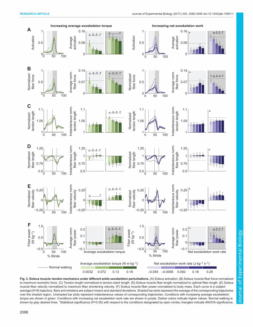
Effects of increasing average exoskeleton torque onlocomotor coordinationExoskeleton-side soleus muscle–tendon mechanicsAs exoskeleton average torque was independently increased, themechanics of the soleus muscle–tendon unit at the assisted anklejoint were disrupted. Average exoskeleton-side soleus muscleactivation decreased by 69% during mid-stance and by 21%during late stance across exoskeleton torque conditions (P=8×10–3

and P=0.02, respectively; Fig. 3A). Average exoskeleton-sidesoleus muscle fiber force decreased by 65% during mid-stance andby 45% during late stance across exoskeleton torque conditions(P=8×10–3 and P=2×10–5, respectively; Fig. 3B). Change in tendonlength, from the instant the soleus muscle fiber started lengtheningto the instant it transitioned from lengthening to shortening,decreased by 74% across exoskeleton torque conditions (P=1×10–3;Fig. 3C). Soleus muscle fiber length, at the instant the soleus muscletransitioned from lengthening to shortening, increased by 12% andmuscle fiber contraction velocity, at the instant of peak muscle fiberpower, increased by 155% across exoskeleton torque conditions(P=1×10–3 and P=0.02, respectively; Fig. 3D,E). Positive musclefiber work during late stance increased by 232% across exoskeletontorque conditions (P=0.01; Fig. 3F). Similar trends were observed inthe medial and lateral gastrocnemius muscles for a majority of theseoutcomes, but to a lesser extent (see Appendix, Figs A1, A2).

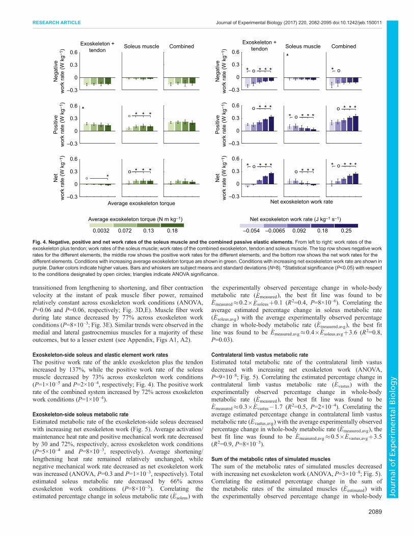
Exoskeleton-side soleus and elastic element work ratesThe positive work rate of the exoskeleton plus tendon decreasedwith increasing average exoskeleton torque (ANOVA, P=2×10–3;Fig. 4) while the positive work rate of the soleus muscle increasedby 142% across exoskeleton torque conditions (P=0.02). Thepositive work rate of the combined exoskeleton, tendon and soleusmuscle remained relatively unchanged as exoskeleton torque wasincreased (ANOVA, P=0.9).

Exoskeleton-side soleus metabolic rateThe trend in estimated metabolic rate of the exoskeleton-side soleusas average exoskeleton torque was increased appeared to be similar

to the trend in measured whole-body metabolic rate (Fig. 5).Average activation/maintenance heat rate decreased by 28% acrossexoskeleton torque conditions (P=2×10–3). Average shortening/lengthening heat rate appeared to increase with increasing averageexoskeleton torque, but the trend was not significant (ANOVA,P=0.1). Positive mechanical work rate increased by 144% from thecondition with no exoskeleton torque to the condition withthe second-highest exoskeleton torque (P=8×10–3). Correlatingthe estimated percentage change in soleus metabolic rate ( _Esoleus)with the experimentally observed percentage change in whole-bodymetabolic rate ( _Emeasured), the best fit line was found to be_Emeasured�0:1� _Esoleusþ5:0 (R2=0.3, P=2×10–3). Correlating theaverage estimated percentage change in soleus metabolic rate( _Esoleus;avg) with the average experimentally observed percentagechange in whole-body metabolic rate ( _Emeasured;avg), the best fitline was found to be _Emeasured;avg�0:2� _Esoleus;avgþ0:1 (R2=0.8,P=0.1).

Contralateral limb vastus metabolic rateEstimated metabolic rate of the contralateral limb vastus increasedwith increasing average exoskeleton torque (ANOVA, P=0.02;Fig. 5) and matched trends in measured whole-body metabolic rate.Correlating the estimated percentage change in contralateral limbvastus metabolic rate ( _Evastus) with the experimentally observedpercentage change in whole-body metabolic rate ( _Emeasured), the bestfit line was found to be _Emeasured�0:2� _Evastusþ1:2 (R2=0.8,P=2×10–8). Correlating the average estimated percentage change incontralateral limb vastus metabolic rate ( _Evastus;avg) with the averageexperimentally observed percentage change in whole-bodymetabolic rate ( _Emeasured;avg), the best fit line was found to be_Emeasured;avg�0:2� _Evastus;avgþ1:0 (R2=0.9, P=0.05).

Sum of the metabolic rates of simulated musclesThe trend in the sum of the metabolic rates of simulated muscleswith increasing average exoskeleton torque was similar to the trendobserved in measured whole-body metabolic rate (Fig. 5).Correlating the estimated percentage change in the sum of themetabolic rates of the simulated muscles ( _Eestimated) with theexperimentally observed percentage change in whole-bodymetabolic rate ( _Emeasured), the best fit line was found to be_Emeasured�0:4� _Eestimatedþ3:4 (R2=0.6, P=7×10–8). Correlatingthe average estimated percentage change in the sum of themetabolic rates of the simulated muscles ( _Eestimated;avg) with theaverage experimentally observed percentage change in whole-bodymetabolic rate ( _Emeasured;avg), the best fit line was found to be_Emeasured;avg�0:7� _Eestimated;avg�3:4 (R2=0.9, P=0.02).

Effects of increasing net exoskeleton work on locomotorcoordinationExoskeleton-side soleus muscle-tendon mechanicsEffort-related measures of the assisted soleus decreased withincreasing net exoskeleton work. Average exoskeleton-side soleusmuscle activation and fiber force during mid-stance increased as netexoskeletonwork was increased (ANOVA,P=8×10–3 andP=3×10–3,respectively; Fig. 3A,B). Average exoskeleton-side soleus muscleactivation and fiber force during late stance decreased by 66 and 73%,respectively, across exoskeleton work conditions (P=5×10–6 andP=2×10–6, respectively). Change in tendon length, from the instantthe soleus muscle started lengthening to the instant it transitionedfrom lengthening to shortening, remained relatively unchanged asnet exoskeleton work was increased (ANOVA, P=0.2; Fig. 3C).Soleus muscle fiber length, at the instant the soleus muscle

2087


Journal

ofEx

perim

entalB

iology

http://jeb.biologists.org/lookup/doi/10.1242/jeb.150011.supplemental


0 50 1000

0.5

1

0 50 100

0 50 100

0 50 100

0 50 100

0 50 100

0 50 100% Stride

0 50 100

0 50 100

0 50 100

0 50 100

0 50 100% Stride

Act

ivat

ion

0

0.08

0.16

Aver

age

activ

atio

n

0

0.5

1

Act

ivat

ion

0

0.08

0.16

Aver

age

activ

atio

n

0

0.5

1

Nor

mal

ized

fiber

forc

e

0

0.07

0.14Av

erag

e no

rm.

fiber

forc

e

0

0.5

1

Nor

mal

ized

fiber

forc

e

0

0.07

0.14

Aver

age

norm

.fib

er fo

rce

1

1.05

1.1

Nor

mal

ized

tend

on le

ngth

1

1.05

1.1

Inst

anta

neou

s no

rm.

tend

on le

ngth

1

1.05

1.1

Nor

mal

ized

tend

on le

ngth

1

1.05

1.1

Inst

anta

neou

s no

rm.

tend

on le

ngth

0.5

0.75

1

1.25

Nor

mal

ized

fiber

leng

th

0.5

0.75

1

1.25

Inst

anta

neou

s no

rm.

fiber

leng

th

0.5

0.75

1

1.25

Nor

mal

ized

fiber

leng

th

0.5

0.75

1

1.25

Inst

anta

neou

s no

rm.

fiber

leng

th

−0.25

0

0.25

Nor

mal

ized

fiber

vel

ocity

−0.25

0

0.25

Inst

anta

neou

s no

rm.

fiber

vel

ocity

−0.25

0

0.25

Nor

mal

ized

fiber

vel

ocity

−0.25

0

0.25

Inst

anta

neou

s no

rm.

fiber

vel

ocity

−0.5

0.5

1.5

Fibe

r pow

er(W

kg−

1 )

−0.1

0

0.1

0.2

Aver

age

norm

.fib

er p

ower

Average exoskeleton torque−0.5

0.5

1.5

Fibe

r pow

er(W

kg−

1 )

−0.1

0

0.1

0.2

Aver

age

norm

.fib

er p

ower

Net exoskeleton work rate

* * *o

* * *o * * *o

Increasing net exoskeleton workIncreasing average exoskeleton torque

* * *o

* * * *o

o

0.0032 0.072 0.13 0.18


–0.054 –0.0065 0.092 0.18 0.25


A

B

C

D

E

F

* * *o

* * *o

* * *o

Normal walking

*o

*o

* * * * * *o

Fig. 3. Soleusmuscle–tendonmechanics under different ankle exoskeleton perturbations. (A) Soleus activation. (B) Soleus muscle fiber force normalizedto maximum isometric force. (C) Tendon length normalized to tendon slack length. (D) Soleus muscle fiber length normalized to optimal fiber length. (E) Soleusmuscle fiber velocity normalized to maximum fiber shortening velocity. (F) Soleus muscle fiber power normalized to body mass. Each curve is a subjectaverage (N=8) trajectory. Bars andwhiskers are subject means and standard deviations. Shaded bar plots represent the average of the corresponding trajectoriesover the shaded region. Unshaded bar plots represent instantaneous values of corresponding trajectories. Conditions with increasing average exoskeletontorque are shown in green. Conditions with increasing net exoskeleton work rate are shown in purple. Darker colors indicate higher values. Normal walking isshown by gray dashed lines. *Statistical significance (P<0.05) with respect to the conditions designated by open circles; triangles indicate ANOVA significance.

2088


Journal

ofEx

perim

entalB

iology

transitioned from lengthening to shortening, and fiber contractionvelocity at the instant of peak muscle fiber power, remainedrelatively constant across exoskeleton work conditions (ANOVA,P=0.06 and P=0.06, respectively; Fig. 3D,E). Muscle fiber workduring late stance decreased by 77% across exoskeleton workconditions (P=8×10–3; Fig. 3E). Similar trends were observed in themedial and lateral gastrocnemius muscles for a majority of theseoutcomes, but to a lesser extent (see Appendix, Figs A1, A2).

Exoskeleton-side soleus and elastic element work ratesThe positive work rate of the ankle exoskeleton plus the tendonincreased by 137%, while the positive work rate of the soleusmuscle decreased by 73% across exoskeleton work conditions(P=1×10–5 and P=2×10–4, respectively; Fig. 4). The positive workrate of the combined system increased by 72% across exoskeletonwork conditions (P=1×10–4).

Exoskeleton-side soleus metabolic rateEstimated metabolic rate of the exoskeleton-side soleus decreasedwith increasing net exoskeleton work (Fig. 5). Average activation/maintenance heat rate and positive mechanical work rate decreasedby 30 and 72%, respectively, across exoskeleton work conditions(P=5×10–4 and P=8×10–3, respectively). Average shortening/lengthening heat rate remained relatively unchanged, whilenegative mechanical work rate decreased as net exoskeleton workwas increased (ANOVA, P=0.3 and P=1×10–3, respectively). Totalestimated soleus metabolic rate decreased by 66% acrossexoskeleton work conditions (P=8×10–3). Correlating theestimated percentage change in soleus metabolic rate ( _Esoleus) with

the experimentally observed percentage change in whole-bodymetabolic rate ( _Emeasured), the best fit line was found to be_Emeasured�0:2� _Esoleusþ0:1 (R2=0.4, P=8×10–6). Correlating theaverage estimated percentage change in soleus metabolic rate( _Esoleus;avg) with the average experimentally observed percentagechange in whole-body metabolic rate ( _Emeasured;avg), the best fitline was found to be _Emeasured;avg�0:4� _Esoleus;avgþ3:6 (R2=0.8,P=0.03).

Contralateral limb vastus metabolic rateEstimated total metabolic rate of the contralateral limb vastusdecreased with increasing net exoskeleton work (ANOVA,P=9×10–8; Fig. 5). Correlating the estimated percentage change incontralateral limb vastus metabolic rate ( _Evastus) with theexperimentally observed percentage change in whole-bodymetabolic rate ( _Emeasured), the best fit line was found to be_Emeasured�0:3� _Evastus�1:7 (R2=0.5, P=2×10–4). Correlating theaverage estimated percentage change in contralateral limb vastusmetabolic rate ( _Evastus;avg) with the average experimentally observedpercentage change in whole-body metabolic rate ( _Emeasured;avg), thebest fit line was found to be _Emeasured;avg�0:5� _Evastus;avgþ3:5(R2=0.9, P=8×10–3).

Sum of the metabolic rates of simulated musclesThe sum of the metabolic rates of simulated muscles decreasedwith increasing net exoskeleton work (ANOVA, P=3×10–8; Fig. 5).Correlating the estimated percentage change in the sum ofthe metabolic rates of the simulated muscles ( _Eestimated) withthe experimentally observed percentage change in whole-body

0.0032 0.072 0.13 0.18 0.250.180.092–0.0065–0.054


–0.3

0

0.3

0.6Exoskeleton +

tendonSoleus muscle Combined

Exoskeleton +tendon Soleus muscle Combined

Average exoskeleton torque Net exoskeleton work rate

Neg

ativ

ew

ork

rate

(W k

g−1 )

Pos

itive

wor

k ra

te (W

kg−

1 )N

etw

ork

rate

(W k

g−1 )

Neg

ativ

ew

ork

rate

(W k

g−1 )

Pos

itive

wor

k ra

te (W

kg−

1 )N

etw

ork

rate

(W k

g−1 )

–0.3

0

0.3

0.6

–0.3

0

0.3

0.6

–0.3

0

0.3

0.6

–0.3

0

0.3

0.6

–0.3

0

0.3

0.6

* * *o

* * *o*o

* * * *o

* * *o

* * * *o

* * * *o

* * *o

* o

* * *o

* * * *o


Fig. 4. Negative, positive and net work rates of the soleus muscle and the combined passive elastic elements. From left to right: work rates of theexoskeleton plus tendon; work rates of the soleus muscle; work rates of the combined exoskeleton, tendon and soleus muscle. The top row shows negative workrates for the different elements, the middle row shows the positive work rates for the different elements, and the bottom row shows the net work rates for thedifferent elements. Conditions with increasing average exoskeleton torque are shown in green. Conditions with increasing net exoskeleton work rate are shown inpurple. Darker colors indicate higher values. Bars and whiskers are subject means and standard deviations (N=8). *Statistical significance (P<0.05) with respectto the conditions designated by open circles; triangles indicate ANOVA significance.

2089


Journal

ofEx

perim

entalB

iology

metabolic energy consumption ( _Emeasured), the best fit line wasfound to be _Emeasured�0:5� _Eestimated�1:1 (R2=0.5, P=1×10–7).Correlating the average estimated percentage change in the sum ofthe metabolic rates of the simulated muscles ( _Eestimated;avg) with theaverage experimentally observed percentage change in whole-bodymetabolic rate ( _Emeasured;avg), the best fit line was found to be_Emeasured;avg�0:8� _Eestimated;avgþ2:4 (R2=0.9, P=6×10–3).

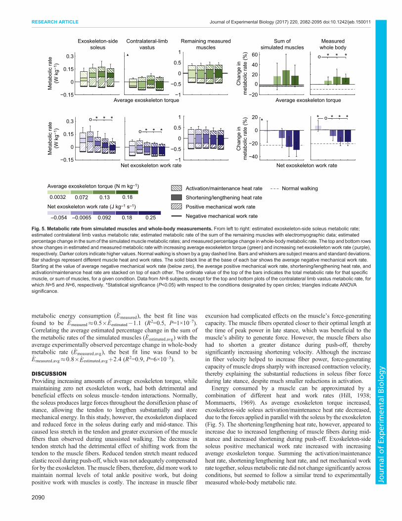
DISCUSSIONProviding increasing amounts of average exoskeleton torque, whilemaintaining zero net exoskeleton work, had both detrimental andbeneficial effects on soleus muscle–tendon interactions. Normally,the soleus produces large forces throughout the dorsiflexion phase ofstance, allowing the tendon to lengthen substantially and storemechanical energy. In this study, however, the exoskeleton displacedand reduced force in the soleus during early and mid-stance. Thiscaused less stretch in the tendon and greater excursion of the musclefibers than observed during unassisted walking. The decrease intendon stretch had the detrimental effect of shifting work from thetendon to the muscle fibers. Reduced tendon stretch meant reducedelastic recoil during push-off, which was not adequately compensatedfor by the exoskeleton. Themuscle fibers, therefore, did morework tomaintain normal levels of total ankle positive work, but doingpositive work with muscles is costly. The increase in muscle fiber

excursion had complicated effects on the muscle’s force-generatingcapacity. The muscle fibers operated closer to their optimal length atthe time of peak power in late stance, which was beneficial to themuscle’s ability to generate force. However, the muscle fibers alsohad to shorten a greater distance during push-off, therebysignificantly increasing shortening velocity. Although the increasein fiber velocity helped to increase fiber power, force-generatingcapacity of muscle drops sharply with increased contraction velocity,thereby explaining the substantial reductions in soleus fiber forceduring late stance, despite much smaller reductions in activation.

Energy consumed by a muscle can be approximated by acombination of different heat and work rates (Hill, 1938;Mommaerts, 1969). As average exoskeleton torque increased,exoskeleton-side soleus activation/maintenance heat rate decreased,due to the forces applied in parallel with the soleus by the exoskeleton(Fig. 5). The shortening/lengthening heat rate, however, appeared toincrease due to increased lengthening of muscle fibers during mid-stance and increased shortening during push-off. Exoskeleton-sidesoleus positive mechanical work rate increased with increasingaverage exoskeleton torque. Summing the activation/maintenanceheat rate, shortening/lengthening heat rate, and net mechanical workrate together, soleusmetabolic rate did not change significantly acrossconditions, but seemed to follow a similar trend to experimentallymeasured whole-body metabolic rate.

* * * *o

−40

−20

0

20

−0.15

0

0.15

0.3

−1

−0.5

0

0.5

1

−20

0

20

40

60

−0.15

0

0.15

0.3

−1

−0.5

0

0.5

1M

etab

olic

rate

(W k

g−1 )

Exoskeleton-sidesoleus

Average exoskeleton torque

Contralateral-limbvastus

Average exoskeleton torque

Sum ofsimulated muscles

Measuredwhole body

Met

abol

ic ra

te(W

kg−

1 )


Cha

nge

inm

etab

olic

rate

(%)

Remaining measuredmuscles

Cha

nge

inm

etab

olic

rate

(%)

0.0032 0.072 0.13 0.18


–0.054 –0.0065 0.092 0.18 0.25


Activation/maintenance heat rate

Shortening/lengthening heat rate

Positive mechanical work rate

Negative mechanical work rate

* * *o

* * *o

* * *o

Normal walking


Fig. 5. Metabolic rate from simulated muscles and whole-body measurements. From left to right: estimated exoskeleton-side soleus metabolic rate;estimated contralateral limb vastus metabolic rate; estimated metabolic rate of the sum of the remaining muscles with electromyographic data; estimatedpercentage change in the sumof the simulatedmusclemetabolic rates; andmeasured percentage change in whole-bodymetabolic rate. The top and bottom rowsshow changes in estimated and measured metabolic rate with increasing average exoskeleton torque (green) and increasing net exoskeleton work rate (purple),respectively. Darker colors indicate higher values. Normal walking is shown by a gray dashed line. Bars and whiskers are subject means and standard deviations.Bar shadings represent different muscle heat and work rates. The solid black line at the base of each bar shows the average negative mechanical work rate.Starting at the value of average negative mechanical work rate (below zero), the average positive mechanical work rate, shortening/lengthening heat rate, andactivation/maintenance heat rate are stacked on top of each other. The ordinate value of the top of the bars indicates the total metabolic rate for that specificmuscle, or sum of muscles, for a given condition. Data from N=8 subjects, except for the top and bottom plots of the contralateral limb vastus metabolic rate, forwhich N=5 and N=6, respectively. *Statistical significance (P<0.05) with respect to the conditions designated by open circles; triangles indicate ANOVAsignificance.

2090


Journal

ofEx

perim

entalB

iology

Reductions in the elastic recoil in the tendon, as well as increasedlengthening and shortening of the soleus muscle fibers, negatedthe reductions in muscle activation and fiber force afforded by theexoskeleton. The human-robot system proved less efficient than thehuman system alone. Similar changes in soleus muscle–tendonmechanics were also observed during hopping with passive ankleexoskeletons (Farris et al., 2014); plantarflexor muscle fiberforce decreased when passive assistance was provided, but fibershortening velocity increased, resulting in no significant change inpositivemuscle fiberwork. Such trade-offs in the observed changes inplantarflexor muscle–tendon mechanics led the metabolic rate of theplantarflexormuscles to remain relatively constantwhenhoppingwithandwithout assistance,which is comparable toour results forwalking.Hopping with passive ankle exoskeleton assistance, however, still ledto a reduction in whole-body energy consumption, likely due to off-loadingof othermuscle forces, particularlyabout the knee joint (Farriset al., 2014). Simulations of a simple, lumped model of theplantarflexor muscle–tendon units during walking with an elasticankle exoskeleton also showed similar results: increasing exoskeletonstiffness decreased activation and force of the plantarflexor musclefibers, but increasedmuscle fiber length changes and led to no changein work done by the muscle fibers (Sawicki and Khan, 2016). Incontrast with our results, this simulation study showed thatplantarflexor muscle metabolic rate decreased with increasingexoskeleton stiffness. This could be a result of differences in theway in which exoskeleton torque was applied in our study comparedwith Sawicki (2016), a result of different changes elsewhere in thebody, or a result of different constraints on joint kinematics. In general,it seems the soleus muscle–tendon unit is sensitive to changes inoperation. Slight alterations to the nominal systemcan have significanteffects on coordination, which can be beneficial or detrimental toindividual muscle and whole-body metabolic energy consumption,depending on the specific task.As average exoskeleton torque was increased, changes in

contralateral limb vastus mechanics and energetics were observed,which helps further explain the increase in experimentally measuredwhole-body metabolic rate. Changes in estimated contralateral limbvastus metabolic rate correlated well with experimentally observedchanges in whole-body metabolic rate. Summing the metabolic rateof each muscle for which we had electromyographic data, we foundthat trends matched experimentally observed trends in whole-bodymetabolic rate well (Fig. 5).Joint work is not necessarily a good predictor of muscle work and,

consequently, energy consumed by a muscle. Positive exoskeleton-side soleus muscle fiber work increased with increasing averageexoskeleton torque, but the biological ankle joint work remainedrelatively unchanged according to the muscle-generated ankle jointwork computations, and actually decreased according to the inversedynamics-derived ankle joint work computations.Changing the amount of net work the exoskeleton provided also

impacted exoskeleton-side soleus muscle mechanics and energetics,but in ways that were more expected. With increasing netexoskeleton work, peak exoskeleton-applied torque occurred laterin stance, leading to significant changes in muscle–tendondynamics. Reduced activation, in addition to reduced positivepower during late stance, resulted in reduced effort of the soleus(Fig. 3A). Soleus muscle fiber force (Fig. 3B) and work (Fig. 3F)were reduced as net exoskeleton work was increased, therebycompromising the normal capabilities of the biological ankle.Positive work provided by the exoskeleton more than compensatedfor the reduced performance of the biological mechanisms, leadingto an improved human-robot cooperative system. Metabolic rate of

the exoskeleton-side soleus muscle significantly decreased withincreasing net exoskeleton work, which accounted for a portion ofthe reduction in whole-body energy expenditure (Fig. 5).

As net exoskeleton work was increased, changes in contralaterallimb vastus mechanics and energetics were observed, helping tofurther explain reductions in experimentally measured whole-bodymetabolic rate. Decreases in exoskeleton-side soleus metabolic ratewere greater than those observed in the contralateral limb vastus, butboth contributed to reductions in whole-body metabolic rate.Summing the metabolic rate of each muscle for which we hadelectromyographic data, trends fit experimentally observedreductions in whole-body metabolic rate well (Fig. 5).

Tendon stiffness and other muscle–tendon properties seem to betuned such that the biological ankle joint operates efficiently. Theresults of this study support the idea that the physiological valueof the Achilles tendon stiffness is optimal for muscle efficiencyduring walking and running (Lichtwark and Wilson, 2007). Thelengthening and shortening of the Achilles tendon, instead of themuscle fibers, allows for energy to be stored and returned passivelythroughout stance. Positive work done by elastic elements canreduce the amount of positive work done by muscles.

Usefully interacting with biological muscles and tendons, via anexternal device, is complicated. Muscle–tendon mechanics areimportant and should be taken into account when designingdevices to assist human motion. Adding an external device to thehuman body may affect muscle-level mechanics and energetics inunexpected ways. Disrupted muscle–tendon interactions wereobserved in this study and have similarly been observed in humanhopping with ankle exoskeletons (Farris et al., 2013, 2014). Assistivedevices should be designed and controlled to compensate for anycompromised performance or functioning of muscles and tendons.Analyses similar to those discussed above can be used to helpunderstand how different exoskeleton behaviors affect muscle-levelmechanics, and provide insights intowhy certain device behaviors aremore effective than others at assisting locomotion. For instance,torque support with a device can be an effective assistance strategy(Collins et al., 2015), but subtleties of how the external torques areapplied and how the device interacts with the human musculoskeletalsystem greatly impact coordination patterns and overall effectiveness.

The modelling approaches used in this study can be applied to awide array of human motions. The results suggest that, given acoordination pattern, via measured muscle activity and jointkinematics, it is possible to generate reasonable estimates ofindividual muscle mechanics and metabolic rate. In the future it maybe possible to invert the process. Based on what we know about themechanics and energetics of individual muscles, we can try togenerate a set of desirable coordination patterns. It may even bepossible to prescribe exoskeleton behaviors that elicit desirablechanges in coordination.

Our modelling and simulation approach required making anumber of assumptions and choices that need to be considered whenevaluating the generated results. If the parameters used in the modelwere inaccurate, this could have led to invalid estimates of musclemechanics and energetics. The parameters we used are, however,comparable to previously published work (Arnold et al., 2000,2010) which is based on cadaver studies (Ward et al., 2009).Furthermore, to validate our approach, we compared muscle-generated ankle joint moments and powers to inverse dynamics-derived ankle joint moments and powers (Fig. 2). We optimizedparameters to reduce the RMSE between the two, and performed anin-depth sensitivity analysis (Figs S1–S6) which shows thequalitative trends are robust to model parameters.

2091


Journal

ofEx

perim

entalB

iology


0 50 1000

0.5

1

0 50 100

0 50 100

0 50 100

0 50 100

0 50 100% Stride

0 50 100% Stride

0 50 100

0 50 100

0 50 100

0 50 100

0 50 100

Act

ivat

ion

0

0.05

0.1

Aver

age

activ

atio

n

0

0.5

1

Act

ivat

ion

0

0.05

0.1

Aver

age

activ

atio

n

0

0.5

1

Nor

mal

ized

fiber

forc

e

0

0.03

0.06Av

erag

e no

rm.

fiber

forc

e

0

0.5

1

Nor

mal

ized

fiber

forc

e

0

0.03

0.06

Aver

age

norm

.fib

er fo

rce

0.93

1

1.07

Nor

mal

ized

tend

on le

ngth

0.93

1

1.07

Inst

anta

neou

s no

rm.

tend

on le

ngth

0.93

1

1.07

Nor

mal

ized

tend

on le

ngth

0.93

1

1.07

Inst

anta

neou

s no

rm.

tend

on le

ngth

0.2

0.6

1

1.4

Nor

mal

ized

fiber

leng

th

0.2

0.6

1

1.4

Inst

anta

neou

s no

rm.

fiber

leng

th

0.2

0.6

1

1.4

Nor

mal

ized

fiber

leng

th

0.2

0.6

1

1.4

Inst

anta

neou

s no

rm.

fiber

leng

th

−0.4

0

0.4

Nor

mal

ized

fiber

vel

ocity

−0.3

0

0.3

Inst

anta

neou

s no

rm.

fiber

vel

ocity

−0.4

0

0.4

Nor

mal

ized

fiber

vel

ocity

−0.3

0

0.3

Inst

anta

neou

s no

rm.

fiber

vel

ocity

−0.2

0

0.2

Fibe

r pow

er(W

kg−

1 )

−0.03

0

0.03

0.06

Aver

age

norm

.fib

er p

ower


0

0.2

Fibe

r pow

er(W

kg−

1 )

−0.03

0

0.03

0.06

Aver

age

norm

.fib

er p

ower



0.0032 0.072 0.13 0.18


–0.054 –0.0065 0.092 0.18 0.25


A

B

C

D

E

F

Normal walking

*o

* * *o

Fig. A1. Medial gastrocnemius muscle–tendon mechanics under different ankle exoskeleton perturbations. Trends in medial gastrocnemius muscle–tendon mechanics closely matched those of the soleus. (A) Medial gastrocnemius activation. (B) Medial gastrocnemius muscle fiber force normalized tomaximum isometric force. (C) Tendon length normalized to tendon slack length. (D) Medial gastrocnemius muscle fiber length normalized to optimal fiber length.(E) Medial gastrocnemius muscle fiber velocity normalized to maximum fiber shortening velocity. (F) Medial gastrocnemius muscle fiber power normalized tobody mass. Each curve is a subject average (N=8) trajectory. Bars and whiskers are subject means and standard deviations. Shaded bar plots represent theaverage of the corresponding trajectories over the shaded region. Unshaded bar plots represent instantaneous values of corresponding trajectories. Conditionswith increasing average exoskeleton torque are shown in green. Conditions with increasing net exoskeleton work rate are shown in purple. Darker colors indicatehigher values. Normal walking is shown by gray dashed lines. *Statistical significance (P<0.05) with respect to the conditions designated by open circles; trianglesindicate ANOVA significance.

2092


Journal

ofEx

perim

entalB

iology

0 50 1000

0.5

1

0 50 100

0 50 100

0 50 100

0 50 100

0 50 100

0 50 100% Stride

0 50 100

0 50 100

0 50 100

0 50 100

0 50 100% Stride

Act

ivat

ion

0

0.05

0.1

Aver

age

activ

atio

n

0

0.5

1

Act

ivat

ion

0

0.05

0.1

Aver

age

activ

atio

n

0

0.5

1

Nor

mal

ized

fiber

forc

e

0

0.03

0.06Av

erag

e no

rm.

fiber

forc

e

0

0.5

1

Nor

mal

ized

fiber

forc

e

0

0.03

0.06

Aver

age

norm

.fib

er fo

rce

0.93

1

1.07

Nor

mal

ized

tend

on le

ngth

0.93

1

1.07

Inst

anta

neou

s no

rm.

tend

on le

ngth

0.93

1

1.07

Nor

mal

ized

tend

on le

ngth

0.93

1

1.07

Inst

anta

neou

s no

rm.

tend

on le

ngth

0.2

0.6

1

1.4

Nor

mal

ized

fiber

leng

th

0.2

0.6

1

1.4

Inst

anta

neou

s no

rm.

fiber

leng

th

0.2

0.6

1

1.4

Nor

mal

ized

fiber

leng

th

0.2

0.6

1

1.4

Inst

anta

neou

s no

rm.

fiber

leng

th

−0.4

0

0.4

Nor

mal

ized

fiber

vel

ocity

−0.3

0

0.3

Inst

anta

neou

s no

rm.

fiber

vel

ocity

−0.4

0

0.4

Nor

mal

ized

fiber

vel

ocity

−0.3

0

0.3In

stan

tane

ous

norm

.fib

er v

eloc

ity

−0.2

0

0.2

Fibe

r pow

er(W

kg−

1 )

−0.03

0

0.03

0.06

Aver

age

norm

.fib

er p

ower


0

0.2

Fibe

r pow

er(W

kg−

1 )

−0.03

0

0.03

0.06

Aver

age

norm

.fib

er p

ower



0.0032 0.072 0.13 0.18

Average exoskeleton torque (N m kg –1)

–0.054 –0.0065 0.092 0.18 0.25

Net exoskeleton work rate (J kg –1 s –1)

A

B

C

D

E

F

Normal walking

*o

* *o

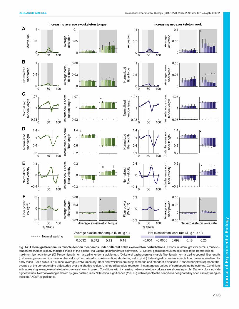
Fig. A2. Lateral gastrocnemius muscle–tendon mechanics under different ankle exoskeleton perturbations. Trends in lateral grastrocnemius muscle–tendon mechanics closely matched those of the soleus. (A) Lateral gastrocnemius activation. (B) Lateral gastrocnemius muscle fiber force normalized tomaximum isometric force. (C) Tendon length normalized to tendon slack length. (D) Lateral gastrocnemius muscle fiber length normalized to optimal fiber length.(E) Lateral gastrocnemius muscle fiber velocity normalized to maximum fiber shortening velocity. (F) Lateral gastrocnemius muscle fiber power normalized tobody mass. Each curve is a subject average (N=5) trajectory. Bars and whiskers are subject means and standard deviations. Shaded bar plots represent theaverage of the corresponding trajectories over the shaded region. Unshaded bar plots represent instantaneous values of corresponding trajectories. Conditionswith increasing average exoskeleton torque are shown in green. Conditions with increasing net exoskeleton work rate are shown in purple. Darker colors indicatehigher values. Normal walking is shown by gray dashed lines. *Statistical significance (P<0.05) with respect to the conditions designated by open circles; trianglesindicate ANOVA significance.

2093


Journal

ofEx

perim

entalB

iology

The soleus, lateral gastrocnemius and medial gastrocnemius wereeach modelled with a separate tendon, as opposed to one sharedtendon. It is unclear which modelling choice is more appropriate forour study, but our fiber and tendon excursions were consistent withexperimental ultrasound studies (Fukunaga et al., 2001; Lichtwarkand Wilson, 2006; Cronin et al., 2010; Rubenson et al., 2012;Cronin et al., 2013). Moreover, qualitative trends in elastic elementnegative, positive and net work (Fig. 4) held for the combination ofall plantarflexor tendons. Combined with the results of oursensitivity analysis, we are confident that this modelling choicedoes not affect our conclusions.We were limited by the number of muscles we could measure

experimentally. In particular, we did not measure muscle activityfrom the glutei, or other muscles acting about the hip, which arethought to consume a substantial amount of energy during walking.Nonetheless, the change in the sum of metabolic energyconsumption from simulated muscles showed a similar trend tothe change in whole-body metabolic energy consumption measuredvia indirect calorimetry; this independent validation increases ourconfidence in the primary findings of the study. Including moremuscles in future experiments would make these analyses morecomplete.Muscle-generated ankle joint mechanics did not perfectly match

inverse dynamics-derived ankle joint mechanics, but most trendswere consistent across the two methods. Results from inversedynamics suggested that total exoskeleton-side positive ankle jointwork decreased as average exoskeleton torque increased, whileresults from the electromyography-driven simulations suggestedthat total exoskeleton-side positive ankle joint work remainedrelatively unchanged. This inconsistency could have implicationsfor our understanding of why contralateral limb knee mechanicsand vastus metabolic rate were affected by torque applied at theexoskeleton-side ankle joint. We only optimized across thoseconditions with increasing average exoskeleton torque, but do notexpect a better match would be obtained if we optimized acrossthose conditions with increasing net exoskeleton work as well.There are inherent trade-offs that prevent errors across all conditionsfrom simultaneously improving. These results illustrate theimportance of knowing the limitations and assumptions inherentin a model and taking these into consideration when analysing andinterpreting its outputs. To account for these limitations, weconducted sensitivity analyses and minimized inconsistenciesbetween inverse dynamics-derived and muscle-generated jointmechanics by optimizing those model parameters in which wehad the least confidence.

ConclusionsWe simulated plantarflexor muscle–tendonmechanics and individualmuscle energetics during walking with an ankle exoskeleton to gain adeeper understanding of how different exoskeleton assistancestrategies affect the operation of the plantarflexor muscles andtendons. Providing increasing amounts of average plantarflexiontorque with an ankle exoskeleton while providing no net work,disrupted soleus muscle–tendon interactions. Reduced tendon recoilwas not sufficiently compensated for by the exoskeleton and this ledto an increase in positive work done by the soleus muscle, which iscostly. Providing increasing amounts of net exoskeleton work morethan compensated for reduced work done by the soleus muscle–tendon unit, leading to a reduction in soleus force, work and totalmetabolic rate. Trends in the sum of the metabolic rates of thesimulated muscles correlated well with trends in experimentallyobserved whole-body metabolic rate, suggesting that the mechanical

andmetabolic changes observed in the simulatedmuscles contributedto the measured changes in whole-body metabolic rate.

By performing these analyses we were able to explainexperimentally observed changes in coordination patterns andmetabolic energy consumption. Models without muscles andtendons would not have been able to capture these effects. Due tothe sensitivity of muscle–tendon units to external disturbances,assisting locomotion by placing a device in parallel with muscles ischallenging. When designing assistive devices, it is thereforeimportant to consider how muscle–tendon mechanics might changedue to interactions with the device and to ensure that the devicesufficiently replaces any compromised function of the humanmusculoskeletal system.

APPENDIXThe medial and lateral gastrocnemius muscles, which operate aboutthe ankle joint, were also directly impacted by exoskeleton-appliedassistance. These muscles, however, are biarticular, causing bothplantarflexion of the ankle joint and flexion of the knee joint, andexhibit behaviors slightly different from the soleus muscle duringnormal walking. To deepen our understanding of how ankleexoskeletons affect those muscles involved in plantarflexion duringassisted walking, we analyzed the changes in muscle-levelmechanics of the medial and lateral gastrocnemius muscles undervarying levels of exoskeleton assistance. Trends observed in themuscle–tendon mechanics of the medial and lateral gastrocnemiusmuscles were similar to those observed in the soleus muscle–tendonunit for most outcomes, but to a lesser extent (Figs A1, A2).

AcknowledgementsThe authors thank Thomas Uchida for assistance with the OpenSim metabolicsmodel.

Competing interestsThe authors declare no competing or financial interests.

Author contributionsS.H.C., R.W.J., S.L.D. and C.L.D. decided upon the musculoskeletal modellingapproach, R.W.J. performed simulations, C.L.D. assisted with simulations, R.W.J.analysed the data, and R.W.J., S.H.C., C.L.D. and S.L.D. wrote the manuscript.

FundingThis material is based upon work supported by the National Science Foundationunder grant number IIS-1355716 and Graduate Research Fellowship grant numberDGE-114747, and by the National Institutes of Health under grant numbers NIH-P2CHD065690 and NIH-U54EB020405. Deposited in PMC for release after 12months.

Data availabilityData used to generate the results are available from the Dryad Digital Repository:http://dx.doi.org/10.5061/dryad.b640d

Supplementary informationSupplementary information available online athttp://jeb.biologists.org/lookup/doi/10.1242/jeb.150011.supplemental

ReferencesArnold, E. M. and Delp, S. L. (2011). Fibre operating lengths of human lower limb

muscles during walking. Philos. Trans. R. Soc. B Biol. Sci. 366, 1530-1539.Arnold, A. S., Asakawa, D. J. and Delp, S. L. (2000). Do the hamstrings and

adductors contribute to excessive internal rotation of the hip in persons withcerebral palsy? Gait Post. 11, 181-190.

Arnold, E. M., Ward, S. R., Lieber, R. L. and Delp, S. L. (2010). A model of thelower limb for analysis of human movement. J. Biomed. Eng. 38, 269-279.

Arnold, E. M., Hamner, S. R., Seth, A., Millard, M. and Delp, S. L. (2013). Howmuscle fiber lengths and velocities affect muscle force generation as humans walkand run at different speeds. J. Exp. Biol. 216, 2150-2160.

2094


Journal

ofEx

perim

entalB

iology

http://dx.doi.org/10.5061/dryad.b640d




http://dx.doi.org/10.1098/rstb.2010.0345

http://dx.doi.org/10.1098/rstb.2010.0345

http://dx.doi.org/10.1016/S0966-6362(00)00046-1

http://dx.doi.org/10.1016/S0966-6362(00)00046-1

http://dx.doi.org/10.1016/S0966-6362(00)00046-1

http://dx.doi.org/10.1007/s10439-009-9852-5

http://dx.doi.org/10.1007/s10439-009-9852-5

http://dx.doi.org/10.1242/jeb.075697



Bhargava, L. J., Pandy, M. G. and Anderson, F. C. (2004). A phenomenologicalmodel for estimating metabolic energy consumption in muscle contraction.J. Biomech. 37, 81-88.

Biewener, A. A. (1998). Muscle function in vivo: a comparison of muscles used forelastic energy savings versusmuscles used to generatemechanical power.Amer.Zool. 38, 703-717.

Biewener, A. A. and Roberts, T. J. (2000). Muscle and tendon contributions toforce, work, and elastic energy savings: a comparative perspective. Exerc. SportSci. Rev. 28, 99-107.

Buchanan, T. S., Lloyd, D. G., Manal, K. and Besier, T. F. (2005). Estimation ofmuscle forces and joint moments using a forward-inverse dynamics model. Med.Sci. Sports Exer. 37, 1911-1916.

Collins, S. H., Wiggin, M. B. and Sawicki, G. S. (2015). Reducing the energy costof human walking using an unpowered exoskeleton. Nature 522, 212-215.

Conchola, E. C., Thompson, B. J. and Smith, D. B. (2013). Effects ofneuromuscular fatigue on the electromechanical delay of the leg extensors andflexors in young and old men. Eur. J. Appl. Physiol. 113, 2391-2399.

Corcos, D. M., Gottlieb, G. L., Latash, M. L., Almeida, G. L. and Agarwal, G. C.(1992). Electromechanical delay: an experimental artifact. J. Electromyogr.Kinesiol. 2, 59-68.

Cronin, N. J., Peltonen, J., Ishikawa,M., Komi, P. V., Avela, J., Sinkjaer, T., Voigt,M. (2010). Achilles tendon length changes during walking in long-term diabetespatients. Clin. Biomech. 25, 476-482.

Cronin, N. J., Avela, J., Finni, T., Peltonen, J. (2013). Differences in contractilebehaviour between the soleus and medial gastrocnemius muscles during humanwalking. J. Exp. Biol. 216, 909-914.

De Luca, C. J., Gilmore, L. D., Kuznetsov, M. and Roy, S. H. (2010). Filtering thesurface EMG signal: movement artifact and baseline noise contamination.J. Biomech. 43, 1573-1579.

Delp, S. L., Loan, J. P., Hoy, M. G., Zajac, F. E., Topp, E. L. and Rosen, J. M.(1990). An interactive graphics-based model of the lower extremity to studyorthopaedic surgical procedures. Trans. Biomed. Eng. 37, 757-767.

Delp, S. L., Anderson, F. C., Arnold, A. S., Loan, P., Habib, A., John, C. T.,Guendelman, E. and Thelen, D. G. (2007). OpenSim: open-source software tocreate and analyze dynamic simulations of movement. Trans. Biomed. Eng. 54,1940-1950.

Donelan, J. M., Kram, R. and Kuo, A. D. (2002). Mechanical work for step-to-steptransitions is a major determinant of the metabolic cost of human walking. J. Exp.Biol. 205, 3717-3727.

Farris, D. J. and Sawicki, G. S. (2012). Linking the mechanics and energetics ofhopping with elastic ankle exoskeletons. J. Appl. Physiol. 113, 1862-1872.

Farris, D. J., Robertson, B. D. and Sawicki, G. S. (2013). Elastic ankleexoskeletons reduce soleus muscle force but not work in human hopping.J. Appl. Physiol. 115, 579-585.

Farris, D. J., Hicks, J. L., Delp, S. L. and Sawicki, G. S. (2014). Musculoskeletalmodelling deconstructs the paradoxical effects of elastic ankle exoskeletons onplantar-flexor mechanics and energetics during hopping. J. Exp. Biol. 217,4018-4028.

Ferris, D. P., Gordon, K. E. and Sawicki, G. S. (2006). An improved powered ankle-foot orthosis using proportional myoelectric control. Gait Post. 23, 425-428.

Fukunaga, T., Kubo, K., Kawakami, Y., Fukashiro, S., Kanehisa, H. andMaganaris, C. N. (2001). In vivo behaviour of human muscle tendon duringwalking. Proc. R. Soc. Lond. B Biol. Sci. 268, 229-233.

Glantz, S. A. (2012).Primer of Biostatistics, 7th edn, pp. 65–67. NewYork: McGraw-Hill.

Gordon, K. E., Ferris, D. P. and Kuo, A. D. (2009). Metabolic and mechanicalenergy costs of reducing vertical center of mass movement during gait. Arch.Phys. Med. Rehab. 90, 136-144.

Grabowski, A., Farley, C. and Kram, R. (2005). Independent metabolic costs ofsupporting body weight and accelerating body mass during walking. J. Appl.Physiol. 98, 579-583.

Hicks, J. L., Uchida, T.K., Seth, A., Rajagopal,A. andDelp,S. L. (2015). Ismymodelgood enough? Best practices for verification and validation of musculoskeletalmodels and simulations of movement. J. Biomech. Eng. 137, 020905.

Hill, A. V. (1938). The heat of shortening and the dynamic constants of muscle.Proc. R. Soc. Lond. B Biol. Sci. 126, 136-195.

Hug, F., Lacourpaille, L. and Nordez, A. (2011). Electromechanical delaymeasured during a voluntary contraction should be interpreted with caution.Muscle Nerve 44, 838-839.

Ishikawa, M., Komi, P. V., Grey, M. J., Leopla, V. and Bruggemann, G. (2005).Muscle-tendon interaction and elastic energy usage in human walking. J. Appl.Physiol. 99, 603-608.

Jackson, R. W. and Collins, S. H. (2015). An experimental comparison of therelative benefits of work and torque assistance in ankle exoskeletons. J. Appl.Physiol. 119, 541-557.

Jackson, R. W., Dembia, C. L., Delp, S. L. and Collins, S. H. (2017). Data from:Muscle-tendon mechanics explain unexpected effects of exoskeleton assistanceon metabolic rate during walking. Dryad Digital Repository. http://dx.doi.org/10.5061/dryad.b640d

Lichtwark, G. A. and Barclay, C. J. (2010). The influence of tendon compliance onmuscle power output and efficiency during cyclic contractions. J. Exp. Biol. 213,707-714.

Lichtwark, G. A., Wilson, A. M. (2006). Interactions between the humangastrocnemius muscle and the Achilles tendon during incline, level and declinelocomotion. J. Exp. Biol. 209, 4379-4388.

Lichtwark, G. A. andWilson, A. M. (2007). Is achilles tendon compliance optimisedfor maximum muscle efficiency during locomotion? J. Biomech. 40, 1768-1775.

Lichtwark, G. A. and Wilson, A. M. (2008). Optimal muscle fascicle length andtendon stiffness for maximising gastrocnemius efficiency during human walkingand running. J. Theor. Biol. 252, 662-673.

Lloyd, D. G. and Besier, T. F. (2003). An EMG-driven musculoskeletal model toestimate muscle forces and knee joint moments in vivo. J. Biomech. 36, 765-776.

Manal, K., Gravare-Silbernagel, K. and Buchanan, T. S. (2012). A real-time EMG-driven musculoskeletal model of the ankle. Multibody Syst. Dyn. 28, 169-180.

Markowitz, J. andHerr, H. (2016). Human legmodel predicts muscle forces, states,and energetics during walking. PLoS Comput. Biol. 12, e1004912.

Meinders, M., Gitter, A. and Czernieckie, J. M. (1998). The role of ankle plantarflexor muscle work during walking. Scand. J. Rehab. Med. 30, 39-46.

Miller, R. H. (2014). A comparison of muscle energy models for simulating humanwalking in three dimensions. J. Biomech. 47, 1373-1381.

Mommaerts, W. F. H. M. (1969). Energetics of muscular contraction. Physiol. Rev.49, 427-508.

Perry, J. and Burnfield, J. M. (2010). Gait Analysis: Normal and PathologicalFunction, 2nd edn. pp. 53-82. Thorofare, NJ, SLACK Inc.

Roberts, T. J. (2002). The integrated function of muscles and tendons duringlocomotion. Comp. Biochem. Physiol. A 133, 1087-1099.

Roberts, T. J., Marsh, R. L., Weyand, P. G. and Taylor, C. R. (1997). Muscularforce in running turkeys: the economy of minimizing work. Science 275,1113-1115.

Robertson, B. D., Farris, D. J. and Sawicki, G. S. (2014). More is not always better:modeling the effects of elastic exoskeleton compliance on underlying anklemuscle-tendon dynamics. Bioinspir. Biomim. 9, 046018.

Rubenson, J., Pires, N. J., Loi, H. O., Pinniger, G. J. and Shannon, D. G. (2012).On the ascent: the soleus operating length is conserved to the ascending limb ofthe force–length curve across gait mechanics in humans. J. Exp. Biol. 215,3539-3551.

Sawicki, G. S. and Khan, N. S. (2016). A simple model to estimate plantarflexormuscle-tendon mechanics and energetics during walking with elastic ankleexoskeletons. Trans. Biomed. Eng. 63, 914-923.

Taylor, C. R. (2007). Force development during sustained locomotion: adeterminant of gait, speed and metabolic power. J. Biomech. 40, 1768-1775.

Uchida, T. K., Hicks, J. L., Dembia, C. L. and Delp, S. L. (2016). Stretching yourenergetic budget: how tendon compliance affects the metabolic cost of running.PLoS ONE 11, e0150378.

Umberger, B. R. (2010). Stance and swing phase costs in human walking.J. R. Soc. Int. 7, 1329-1340.

Umberger, B. R. and Rubenson, J. (2011). Understanding muscle energetics inlocomotion: new modeling and experimental approaches. Exerc. Sport Sci. Rev.39, 59-67.

Umberger, B. R., Gerritsen, K. G. M. and Martin, P. E. (2003). A model of humanmuscle energy expenditure.Comput. Methods Biomech. Biomed. Eng. 6, 99-111.

Ward, S. R., Eng, C. M., Smallwood, L. H. and Lieber, R. L. (2009). Are currentmeasurements of lower extremity muscle architecture accurate? Clin. Orthop.Relat. Res. 467, 1074-1082.

Winter, D. A. (1990). Biomechanics and Motor Control of Human Movement, 2ndedn. pp. 107-138. John Wiley & Sons, Inc., Toronto, Canada,.

Witte, K. A., Zhang, J., Jackson, R. W. and Collins, S. H. (2015). Design of twolightweight, high-bandwidth torque-controlled ankle exoskeletons. IEEEInternational Conference on Robotics and Automation (ICRA), pp. 1223-1228.

Zajac, F. E., Neptune, R. R. and Kautz, S. A. (2003). Biomechanics and musclecoordination of human walking; Part II: lessons from dynamical simulations andclinical implications. Gait Post. 17, 1-17.

2095


Journal

ofEx

perim

entalB

iology

http://dx.doi.org/10.1016/S0021-9290(03)00239-2

http://dx.doi.org/10.1016/S0021-9290(03)00239-2

http://dx.doi.org/10.1016/S0021-9290(03)00239-2

http://dx.doi.org/10.1093/icb/38.4.703



http://dx.doi.org/10.1249/01.mss.0000176684.24008.6f



http://dx.doi.org/10.1038/nature14288

http://dx.doi.org/10.1038/nature14288

http://dx.doi.org/10.1007/s00421-013-2675-y

http://dx.doi.org/10.1007/s00421-013-2675-y

http://dx.doi.org/10.1007/s00421-013-2675-y

http://dx.doi.org/10.1016/1050-6411(92)90017-D

http://dx.doi.org/10.1016/1050-6411(92)90017-D

http://dx.doi.org/10.1016/1050-6411(92)90017-D




http://dx.doi.org/10.1016/j.jbiomech.2010.01.027



http://dx.doi.org/10.1109/10.102791

http://dx.doi.org/10.1109/10.102791

http://dx.doi.org/10.1109/10.102791

http://dx.doi.org/10.1109/TBME.2007.901024




http://dx.doi.org/10.1152/japplphysiol.00802.2012









http://dx.doi.org/10.1016/j.gaitpost.2005.05.004

http://dx.doi.org/10.1016/j.gaitpost.2005.05.004

http://dx.doi.org/10.1098/rspb.2000.1361



http://dx.doi.org/10.1016/j.apmr.2008.07.014






http://dx.doi.org/10.1115/1.4029304

http://dx.doi.org/10.1115/1.4029304

http://dx.doi.org/10.1115/1.4029304



http://dx.doi.org/10.1002/mus.22139




















http://dx.doi.org/10.1016/j.jtbi.2008.01.018



http://dx.doi.org/10.1016/S0021-9290(03)00010-1

http://dx.doi.org/10.1016/S0021-9290(03)00010-1

http://dx.doi.org/10.1007/s11044-011-9285-4

http://dx.doi.org/10.1007/s11044-011-9285-4

http://dx.doi.org/10.1371/journal.pcbi.1004912

http://dx.doi.org/10.1371/journal.pcbi.1004912

http://dx.doi.org/10.1080/003655098444309

http://dx.doi.org/10.1080/003655098444309



http://dx.doi.org/10.1016/S1095-6433(02)00244-1

http://dx.doi.org/10.1016/S1095-6433(02)00244-1

http://dx.doi.org/10.1126/science.275.5303.1113



http://dx.doi.org/10.1088/1748-3182/9/4/046018

http://dx.doi.org/10.1088/1748-3182/9/4/046018

http://dx.doi.org/10.1088/1748-3182/9/4/046018








http://dx.doi.org/10.1371/journal.pone.0150378



http://dx.doi.org/10.1098/rsif.2010.0084

http://dx.doi.org/10.1098/rsif.2010.0084

http://dx.doi.org/10.1097/JES.0b013e31820d7bc5



http://dx.doi.org/10.1080/1025584031000091678

http://dx.doi.org/10.1080/1025584031000091678

http://dx.doi.org/10.1007/s11999-008-0594-8

http://dx.doi.org/10.1007/s11999-008-0594-8

http://dx.doi.org/10.1007/s11999-008-0594-8

http://dx.doi.org/10.1016/S0966-6362(02)00069-3

http://dx.doi.org/10.1016/S0966-6362(02)00069-3

http://dx.doi.org/10.1016/S0966-6362(02)00069-3

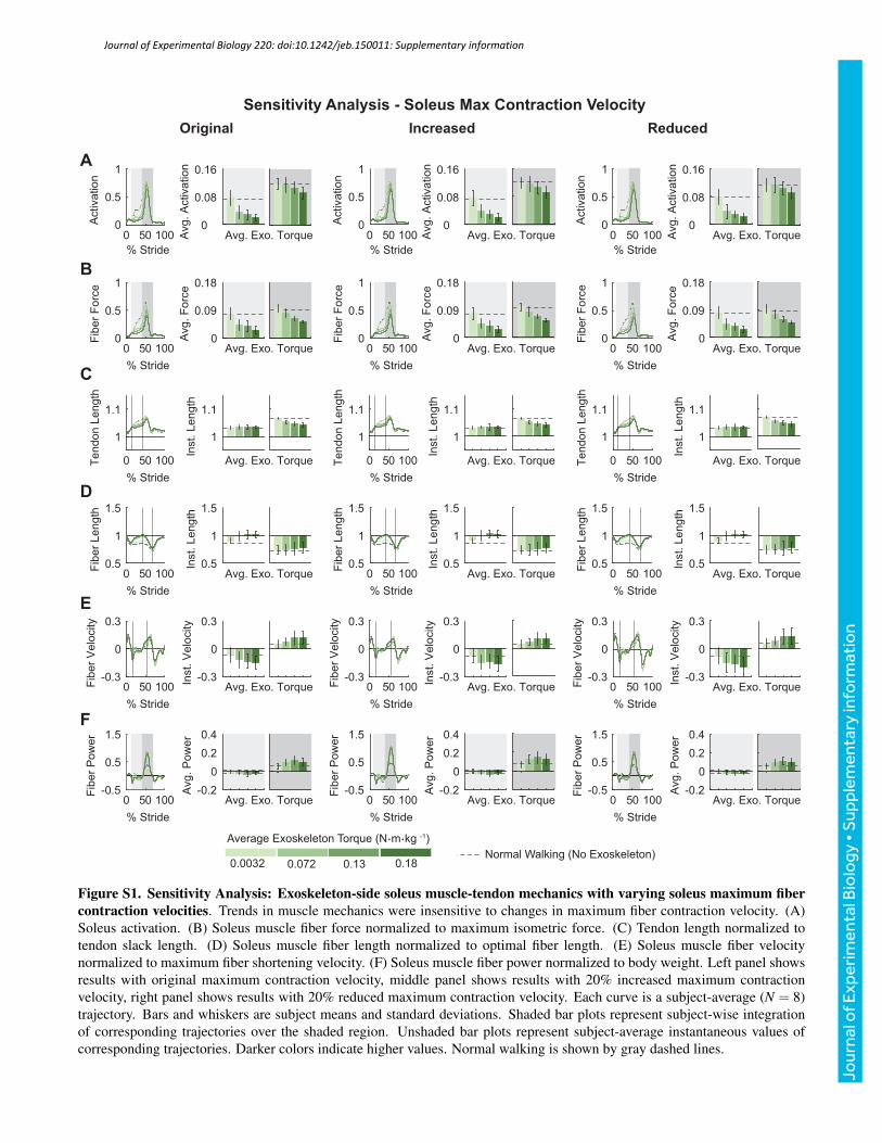
% Stride

0 50 100

Activa

tio

n

0

0.5

1

Avg. Exo. TorqueAvg

. A

ctiva

tio

n

0

0.08

0.16

% Stride

0 50 100

Fib

er

Fo

rce

0

0.5

1

Avg. Exo. Torque

Avg

. F

orc

e

0

0.09

0.18

% Stride

0 50 100Te

nd

on

Le

ng

th

1

1.1

Avg. Exo. Torque

Inst.

Le

ng

th

1

1.1

% Stride

0 50 100

Fib

er

Le

ng

th

0.5

1

1.5

Avg. Exo. Torque

Inst.

Le

ng

th

0.5

1

1.5

% Stride

0 50 100Fib

er

Ve

locity

-0.3

0

0.3

Avg. Exo. Torque

Inst.

Ve

locity

-0.3

0

0.3

% Stride

0 50 100

Fib

er

Po

we

r

-0.5

0.5

1.5

Avg. Exo. Torque

Avg

. P

ow

er

-0.2

0

0.2

0.4

% Stride

0 50 100

Activa

tio

n

0

0.5

1

Avg. Exo. TorqueAvg

. A

ctiva

tio

n

0

0.08

0.16

% Stride

0 50 100F

ibe

r F

orc

e0

0.5

1

Avg. Exo. Torque

Avg

. F

orc

e

0

0.09

0.18

% Stride

0 50 100Te

nd

on

Le

ng

th

1

1.1

Avg. Exo. Torque

Inst.

Le

ng

th1

1.1

% Stride

0 50 100

Fib

er

Le

ng

th

0.5

1

1.5

Avg. Exo. Torque

Inst.

Le

ng

th

0.5

1

1.5

% Stride

0 50 100Fib

er

Ve

locity

-0.3

0

0.3

Avg. Exo. Torque

Inst.

Ve

locity

-0.3

0

0.3

% Stride

0 50 100

Fib

er

Po

we

r

-0.5

0.5

1.5

Avg. Exo. Torque

Avg

. P

ow

er

-0.2

0

0.2

0.4

% Stride

0 50 100

Activa

tio

n

0

0.5

1

Avg. Exo. TorqueAvg

. A

ctiva

tio

n

0

0.08

0.16

% Stride

0 50 100

Fib

er

Fo

rce

0

0.5

1

Avg. Exo. Torque

Avg

. F

orc

e

0

0.09

0.18

% Stride

0 50 100Te

nd

on

Le

ng

th

1

1.1

Avg. Exo. Torque

Inst.

Le

ng

th

1

1.1

% Stride

0 50 100F

ibe

r L

en

gth

0.5

1

1.5

Avg. Exo. Torque

Inst.

Le

ng

th

0.5

1

1.5

% Stride

0 50 100Fib

er

Ve

locity

-0.3

0

0.3

Avg. Exo. TorqueIn

st.

Ve

locity

-0.3

0

0.3

% Stride

0 50 100

Fib

er

Po

we

r

-0.5

0.5

1.5

Avg. Exo. Torque

Avg

. P

ow

er

-0.2

0

0.2

0.4

Original Increased Reduced

0.0032 0.072 0.13 0.18

Average Exoskeleton Torque (N.m.kg -1)

A

B

C

D

E

F

Sensitivity Analysis - Soleus Max Contraction Velocity

Normal Walking (No Exoskeleton)

Figure S1. Sensitivity Analysis: Exoskeleton-side soleus muscle-tendon mechanics with varying soleus maximum fibercontraction velocities. Trends in muscle mechanics were insensitive to changes in maximum fiber contraction velocity. (A)Soleus activation. (B) Soleus muscle fiber force normalized to maximum isometric force. (C) Tendon length normalized totendon slack length. (D) Soleus muscle fiber length normalized to optimal fiber length. (E) Soleus muscle fiber velocitynormalized to maximum fiber shortening velocity. (F) Soleus muscle fiber power normalized to body weight. Left panel showsresults with original maximum contraction velocity, middle panel shows results with 20% increased maximum contractionvelocity, right panel shows results with 20% reduced maximum contraction velocity. Each curve is a subject-average (N = 8)trajectory. Bars and whiskers are subject means and standard deviations. Shaded bar plots represent subject-wise integrationof corresponding trajectories over the shaded region. Unshaded bar plots represent subject-average instantaneous values ofcorresponding trajectories. Darker colors indicate higher values. Normal walking is shown by gray dashed lines.

Journal of Experimental Biology 220: doi:10.1242/jeb.150011: Supplementary information

Jour

nal o

f Exp

erim

enta

l Bio

logy

• S

uppl

emen

tary

info

rmat

ion

% Stride

0 50 100

Activa

tio

n

0

0.5

1

Avg. Exo. TorqueAvg

. A

ctiva

tio

n

0

0.08

0.16

% Stride

0 50 100

Fib

er

Fo

rce

0

0.5

1

Avg. Exo. Torque

Avg

. F

orc

e

0

0.09

0.18

% Stride

0 50 100Te

nd

on

Le

ng

th

1

1.1

Avg. Exo. Torque

Inst.

Le

ng

th

1

1.1

% Stride

0 50 100

Fib

er

Le

ng

th

0.5

1

1.5

Avg. Exo. Torque

Inst.

Le

ng

th

0.5

1

1.5

% Stride

0 50 100Fib

er

Ve

locity

-0.3

0

0.3

Avg. Exo. Torque

Inst.

Ve

locity

-0.3

0

0.3

% Stride

0 50 100

Fib

er

Po

we

r

-0.5

0.5

1.5

Avg. Exo. Torque

Avg

. P

ow

er

-0.2

0

0.2

0.4

% Stride

0 50 100

Activa

tio

n

0

0.5

1

Avg. Exo. TorqueAvg

. A

ctiva

tio

n

0

0.08

0.16

% Stride

0 50 100F

ibe

r F

orc

e0

0.5

1

Avg. Exo. Torque

Avg

. F

orc

e

0

0.09

0.18

% Stride

0 50 100Te

nd

on

Le

ng

th

1

1.1

Avg. Exo. Torque

Inst.

Le

ng

th1

1.1

% Stride

0 50 100

Fib

er

Le

ng

th

0.5

1

1.5

Avg. Exo. Torque

Inst.

Le

ng

th

0.5

1

1.5

% Stride

0 50 100Fib

er

Ve

locity

-0.3

0

0.3

Avg. Exo. Torque

Inst.

Ve

locity

-0.3

0

0.3

% Stride

0 50 100

Fib

er

Po

we

r

-0.5

0.5

1.5

Avg. Exo. Torque

Avg

. P

ow

er

-0.2

0

0.2

0.4

% Stride

0 50 100

Activa

tio

n

0

0.5

1

Avg. Exo. TorqueAvg

. A

ctiva

tio

n

0

0.08

0.16

% Stride

0 50 100

Fib

er

Fo

rce

0

0.5

1

Avg. Exo. Torque

Avg

. F

orc

e

0

0.09

0.18

% Stride

0 50 100Te

nd

on

Le

ng

th

1

1.1

Avg. Exo. Torque

Inst.

Le

ng

th

1

1.1

% Stride

0 50 100F

ibe

r L

en

gth

0.5

1

1.5

Avg. Exo. Torque

Inst.

Le

ng

th

0.5

1

1.5

% Stride

0 50 100Fib

er

Ve

locity

-0.3

0

0.3

Avg. Exo. TorqueIn

st.

Ve

locity

-0.3

0

0.3

% Stride

0 50 100

Fib

er

Po

we

r

-0.5

0.5

1.5

Avg. Exo. Torque

Avg

. P

ow

er

-0.2

0

0.2

0.4


0.0032 0.072 0.13 0.18


A

B

C

D

E

F

Sensitivity Analysis - Soleus Max Isometric Force


Figure S2. Sensitivity Analysis: Exoskeleton-side soleus muscle-tendon mechanics with varying soleus maximum iso-metric forces. Trends in muscle mechanics were insensitive to changes in maximum isometric force. (A) Soleus activation. (B)Soleus muscle fiber force normalized to maximum isometric force. (C) Tendon length normalized to tendon slack length. (D)Soleus muscle fiber length normalized to optimal fiber length. (E) Soleus muscle fiber velocity normalized to maximum fibershortening velocity. (F) Soleus muscle fiber power normalized to body weight. Left panel shows results with original maximumisometric force, middle panel shows results with 10% increased maximum isometric force, right panel shows results with 10%reduced maximum isometric force. Each curve is a subject-average (N = 8) trajectory. Bars and whiskers are subject means andstandard deviations. Shaded bar plots represent subject-wise integration of corresponding trajectories over the shaded region.Unshaded bar plots represent subject-average instantaneous values of corresponding trajectories. Darker colors indicate highervalues. Normal walking is shown by gray dashed lines.


Jour

nal o

f Exp

erim

enta

l Bio

logy

• S

uppl

emen

tary

info

rmat

ion

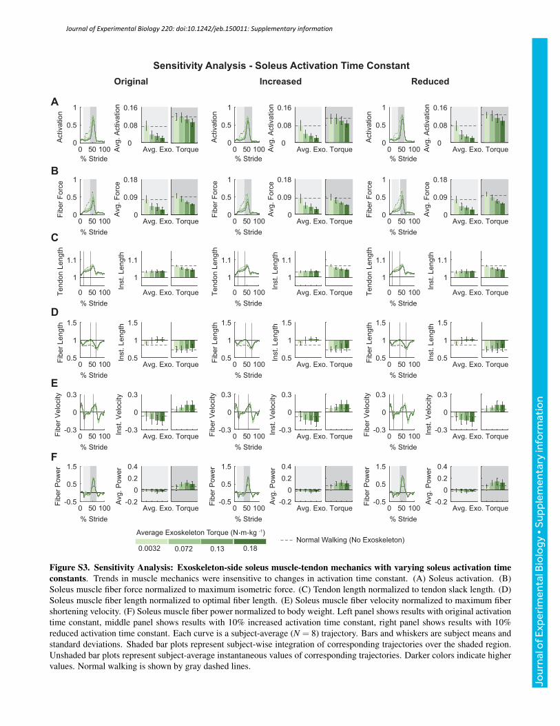
% Stride

0 50 100

Activa

tio

n

0

0.5

1

Avg. Exo. TorqueAvg

. A

ctiva

tio

n

0

0.08

0.16

% Stride

0 50 100

Fib

er

Fo

rce

0

0.5

1

Avg. Exo. Torque

Avg

. F

orc

e

0

0.09

0.18

% Stride

0 50 100Te

nd

on

Le

ng

th

1

1.1

Avg. Exo. Torque

Inst.

Le

ng

th

1

1.1

% Stride

0 50 100

Fib

er

Le

ng

th

0.5

1

1.5

Avg. Exo. Torque

Inst.

Le

ng

th

0.5

1

1.5

% Stride

0 50 100Fib

er

Ve

locity

-0.3

0

0.3

Avg. Exo. Torque

Inst.

Ve

locity

-0.3

0

0.3

% Stride

0 50 100

Fib

er

Po

we

r

-0.5

0.5

1.5

Avg. Exo. Torque

Avg

. P

ow

er

-0.2

0

0.2

0.4

% Stride

0 50 100

Activa

tio

n

0

0.5

1

Avg. Exo. TorqueAvg

. A

ctiva

tio

n

0

0.08

0.16

% Stride

0 50 100F

ibe

r F

orc

e0

0.5

1

Avg. Exo. Torque

Avg

. F

orc

e

0

0.09

0.18

% Stride

0 50 100Te

nd

on

Le

ng

th

1

1.1

Avg. Exo. Torque

Inst.

Le

ng

th1

1.1

% Stride

0 50 100

Fib

er

Le

ng

th

0.5

1

1.5

Avg. Exo. Torque

Inst.

Le

ng

th

0.5

1

1.5

% Stride

0 50 100Fib

er

Ve

locity

-0.3

0

0.3

Avg. Exo. Torque

Inst.

Ve

locity

-0.3

0

0.3

% Stride

0 50 100

Fib

er

Po

we

r

-0.5

0.5

1.5

Avg. Exo. Torque

Avg

. P

ow

er

-0.2

0

0.2

0.4

% Stride

0 50 100

Activa

tio

n

0

0.5

1

Avg. Exo. TorqueAvg

. A

ctiva

tio

n

0

0.08

0.16

% Stride

0 50 100

Fib

er

Fo

rce

0

0.5

1

Avg. Exo. Torque

Avg

. F

orc

e

0

0.09

0.18

% Stride

0 50 100Te

nd

on

Le

ng

th

1

1.1

Avg. Exo. Torque

Inst.

Le

ng

th

1

1.1

% Stride

0 50 100F

ibe

r L

en

gth

0.5

1

1.5

Avg. Exo. Torque

Inst.

Le

ng

th

0.5

1

1.5

% Stride

0 50 100Fib

er

Ve

locity

-0.3

0

0.3

Avg. Exo. TorqueIn

st.

Ve

locity

-0.3

0

0.3

% Stride

0 50 100

Fib

er

Po

we

r

-0.5

0.5

1.5

Avg. Exo. Torque

Avg

. P

ow

er

-0.2

0

0.2

0.4


0.0032 0.072 0.13 0.18


A

B

C

D

E

F

Sensitivity Analysis - Soleus Activation Time Constant


Figure S3. Sensitivity Analysis: Exoskeleton-side soleus muscle-tendon mechanics with varying soleus activation timeconstants. Trends in muscle mechanics were insensitive to changes in activation time constant. (A) Soleus activation. (B)Soleus muscle fiber force normalized to maximum isometric force. (C) Tendon length normalized to tendon slack length. (D)Soleus muscle fiber length normalized to optimal fiber length. (E) Soleus muscle fiber velocity normalized to maximum fibershortening velocity. (F) Soleus muscle fiber power normalized to body weight. Left panel shows results with original activationtime constant, middle panel shows results with 10% increased activation time constant, right panel shows results with 10%reduced activation time constant. Each curve is a subject-average (N = 8) trajectory. Bars and whiskers are subject means andstandard deviations. Shaded bar plots represent subject-wise integration of corresponding trajectories over the shaded region.Unshaded bar plots represent subject-average instantaneous values of corresponding trajectories. Darker colors indicate highervalues. Normal walking is shown by gray dashed lines.


Jour

nal o

f Exp

erim

enta

l Bio

logy

• S

uppl

emen

tary

info

rmat

ion

% Stride

0 50 100

Activa

tio

n

0

0.5

1

Avg. Exo. TorqueAvg

. A

ctiva

tio

n

0

0.08

0.16

% Stride

0 50 100

Fib

er

Fo

rce

0

0.5

1

Avg. Exo. Torque

Avg

. F

orc

e

0

0.09

0.18

% Stride

0 50 100Te

nd

on

Le

ng

th

1

1.1

Avg. Exo. Torque

Inst.

Le

ng

th

1

1.1

% Stride

0 50 100

Fib

er

Le

ng

th

0.5

1

1.5

Avg. Exo. Torque

Inst.

Le

ng

th

0.5

1

1.5

% Stride

0 50 100Fib

er

Ve

locity

-0.3

0

0.3

Avg. Exo. Torque

Inst.

Ve

locity

-0.3

0

0.3

% Stride

0 50 100

Fib

er

Po

we

r

-0.5

0.5

1.5

Avg. Exo. Torque

Avg

. P

ow

er

-0.2

0

0.2

0.4

% Stride

0 50 100

Activa

tio

n

0

0.5

1

Avg. Exo. TorqueAvg

. A

ctiva

tio

n

0

0.08

0.16

% Stride

0 50 100F

ibe

r F

orc

e0

0.5

1

Avg. Exo. Torque

Avg

. F

orc

e

0

0.09

0.18

% Stride

0 50 100Te

nd

on

Le

ng

th

1

1.1

Avg. Exo. Torque

Inst.

Le

ng

th1

1.1

% Stride

0 50 100

Fib

er

Le

ng

th

0.5

1

1.5

Avg. Exo. Torque

Inst.

Le

ng

th

0.5

1

1.5

% Stride

0 50 100Fib

er

Ve

locity

-0.3

0

0.3

Avg. Exo. Torque

Inst.

Ve

locity

-0.3

0

0.3

% Stride

0 50 100

Fib

er

Po

we

r

-0.5

0.5

1.5

Avg. Exo. Torque

Avg

. P

ow

er

-0.2

0

0.2

0.4

% Stride

0 50 100

Activa

tio

n

0

0.5

1

Avg. Exo. TorqueAvg

. A

ctiva

tio

n

0

0.08

0.16

% Stride

0 50 100

Fib

er

Fo

rce

0

0.5

1

Avg. Exo. Torque

Avg

. F

orc

e

0

0.09

0.18

% Stride

0 50 100Te

nd

on

Le

ng

th

1

1.1

Avg. Exo. Torque

Inst.

Le

ng

th

1

1.1

% Stride

0 50 100F

ibe

r L

en

gth

0.5

1

1.5

Avg. Exo. Torque

Inst.

Le

ng

th

0.5

1

1.5

% Stride

0 50 100Fib

er

Ve

locity

-0.3

0

0.3

Avg. Exo. TorqueIn

st.

Ve

locity

-0.3

0

0.3

% Stride

0 50 100

Fib

er

Po

we

r

-0.5

0.5

1.5

Avg. Exo. Torque

Avg

. P

ow

er

-0.2

0

0.2

0.4


0.0032 0.072 0.13 0.18


A

B

C

D

E

F

Sensitivity Analysis - Soleus Tendon Stiffness


Figure S4. Sensitivity Analysis: Exoskeleton-side soleus muscle-tendon mechanics with varying soleus tendon stiffnesses.Trends in muscle mechanics were insensitive to changes in tendon stiffness. (A) Soleus activation. (B) Soleus muscle fiberforce normalized to maximum isometric force. (C) Tendon length normalized to tendon slack length. (D) Soleus muscle fiberlength normalized to optimal fiber length. (E) Soleus muscle fiber velocity normalized to maximum fiber shortening velocity.(F) Soleus muscle fiber power normalized to body weight. Left panel shows results with original tendon strain at maximumisometric force, middle panel shows results with 1% absolute reduction in tendon strain at maximum isometric force, rightpanel shows results with 1% absolute increase in tendon strain at maximum isometric force. Each curve is a subject-average(N = 8) trajectory. Bars and whiskers are subject means and standard deviations. Shaded bar plots represent subject-wiseintegration of corresponding trajectories over the shaded region. Unshaded bar plots represent subject-average instantaneousvalues of corresponding trajectories. Darker colors indicate higher values. Normal walking is shown by gray dashed lines.


Jour

nal o

f Exp

erim

enta

l Bio

logy

• S

uppl

emen

tary

info

rmat

ion

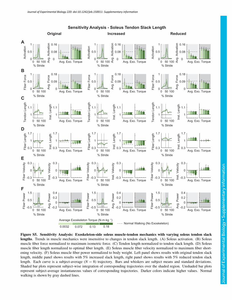
% Stride

0 50 100

Activa

tio

n

0

0.5

1

Avg. Exo. TorqueAvg

. A

ctiva

tio

n

0

0.08

0.16

% Stride

0 50 100

Fib

er

Fo

rce

0

0.5

1

Avg. Exo. Torque

Avg

. F

orc

e

0

0.09

0.18

% Stride

0 50 100Te

nd

on

Le

ng

th

1

1.1

Avg. Exo. Torque

Inst.

Le

ng

th

1

1.1

% Stride

0 50 100

Fib

er

Le

ng

th

0.3

1

1.7

Avg. Exo. Torque

Inst.

Le

ng

th

0.3

1

1.7

% Stride

0 50 100Fib

er

Ve

locity

-0.3

0

0.3

Avg. Exo. Torque

Inst.

Ve

locity

-0.3

0

0.3

% Stride

0 50 100

Fib

er

Po

we

r

-0.5

0.5

1.5

Avg. Exo. Torque

Avg

. P

ow

er

-0.2

0

0.2

0.4

% Stride

0 50 100

Activa

tio

n

0

0.5

1

Avg. Exo. TorqueAvg

. A

ctiva

tio

n

0

0.08

0.16

% Stride

0 50 100F

ibe

r F

orc

e0

0.5

1

Avg. Exo. Torque

Avg

. F

orc

e

0

0.09

0.18

% Stride

0 50 100Te

nd

on

Le

ng

th

1

1.1

Avg. Exo. Torque

Inst.

Le

ng

th1

1.1

% Stride

0 50 100

Fib

er

Le

ng

th

0.3

1

1.7

Avg. Exo. Torque

Inst.

Le

ng

th

0.3

1

1.7

% Stride

0 50 100Fib

er

Ve

locity

-0.3

0

0.3

Avg. Exo. Torque

Inst.

Ve

locity

-0.3

0

0.3

% Stride

0 50 100

Fib

er

Po

we

r

-0.5

0.5

1.5

Avg. Exo. Torque

Avg

. P

ow

er

-0.2

0

0.2

0.4

% Stride

0 50 100

Activa

tio

n

0

0.5

1

Avg. Exo. TorqueAvg

. A

ctiva

tio

n

0

0.08

0.16

% Stride

0 50 100

Fib

er

Fo

rce

0

0.5

1

Avg. Exo. Torque

Avg

. F

orc

e

0

0.09

0.18

% Stride

0 50 100Te

nd

on

Le

ng

th

1

1.1

Avg. Exo. Torque

Inst.

Le

ng

th

1

1.1

% Stride

0 50 100F

ibe

r L

en

gth

0.3

1

1.7

Avg. Exo. Torque

Inst.

Le

ng

th

0.3

1

1.7

% Stride

0 50 100Fib

er

Ve

locity

-0.3

0

0.3

Avg. Exo. TorqueIn

st.

Ve

locity

-0.3

0

0.3

% Stride

0 50 100

Fib

er

Po

we

r

-0.5

0.5

1.5

Avg. Exo. Torque

Avg

. P

ow

er

-0.2

0

0.2

0.4


0.0032 0.072 0.13 0.18


A

B

C

D

E

F

Sensitivity Analysis - Soleus Tendon Slack Length


Figure S5. Sensitivity Analysis: Exoskeleton-side soleus muscle-tendon mechanics with varying soleus tendon slacklengths. Trends in muscle mechanics were insensitive to changes in tendon slack length. (A) Soleus activation. (B) Soleusmuscle fiber force normalized to maximum isometric force. (C) Tendon length normalized to tendon slack length. (D) Soleusmuscle fiber length normalized to optimal fiber length. (E) Soleus muscle fiber velocity normalized to maximum fiber short-ening velocity. (F) Soleus muscle fiber power normalized to body weight. Left panel shows results with original tendon slacklength, middle panel shows results with 5% increased slack length, right panel shows results with 5% reduced tendon slacklength. Each curve is a subject-average (N = 8) trajectory. Bars and whiskers are subject means and standard deviations.Shaded bar plots represent subject-wise integration of corresponding trajectories over the shaded region. Unshaded bar plotsrepresent subject-average instantaneous values of corresponding trajectories. Darker colors indicate higher values. Normalwalking is shown by gray dashed lines.


Jour

nal o

f Exp

erim

enta

l Bio

logy

• S

uppl

emen

tary

info

rmat

ion

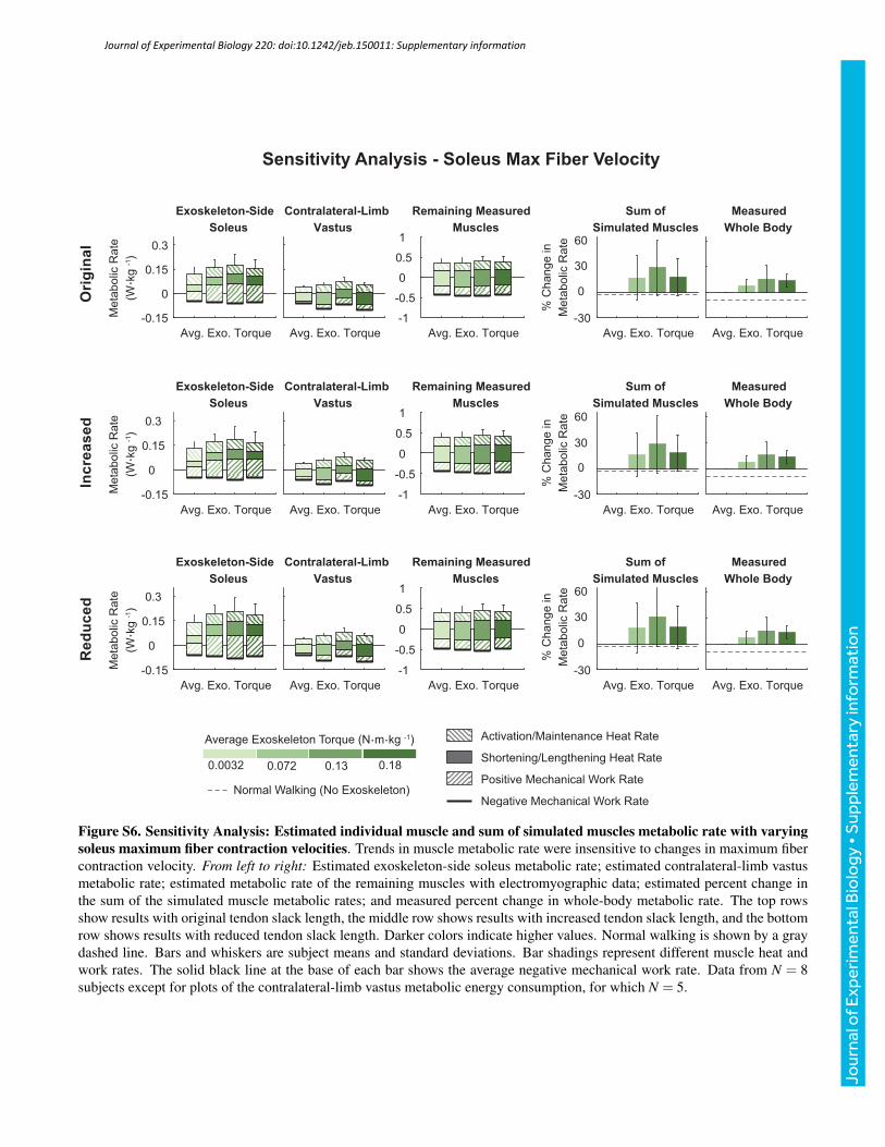
Met

abol

ic R

ate

(W. k

g -1)

-0.15

0

0.15

0.3

Exoskeleton-SideSoleus

Avg. Exo. Torque

Contralateral-LimbVastus

Avg. Exo. Torque-1

-0.5

0

0.5

1

Remaining MeasuredMuscles

Avg. Exo. Torque Avg. Exo. Torque

% C

hang

e in

Met

abol

ic R

ate

-30

0

30

60

Sum ofSimulated Muscles

Avg. Exo. Torque

MeasuredWhole Body

Met

abol

ic R

ate

(W. k

g -1)

-0.15

0

0.15

0.3


Avg. Exo. Torque


Avg. Exo. Torque-1

-0.5

0

0.5

1



% C

hang

e in

Met

abol

ic R

ate

-30

0

30

60

Avg. Exo. Torque

MeasuredWhole Body

Met

abol

ic R

ate

(W. k

g -1)

-0.15

0

0.15

0.3


Avg. Exo. Torque


Avg. Exo. Torque-1

-0.5

0

0.5

1



% C

hang

e in

Met

abol

ic R

ate

-30

0

30

60

Avg. Exo. Torque

MeasuredWhole Body



Sensitivity Analysis - Soleus Max Fiber Velocity

Ori

gina

lIn

crea

sed

Red

uced

0.0032 0.072 0.13 0.18

Average Exoskeleton Torque (N.m.kg -1) Activation/Maintenance Heat Rate

Shortening/Lengthening Heat Rate

Positive Mechanical Work Rate

Negative Mechanical Work RateNormal Walking (No Exoskeleton)

Figure S6. Sensitivity Analysis: Estimated individual muscle and sum of simulated muscles metabolic rate with varyingsoleus maximum fiber contraction velocities. Trends in muscle metabolic rate were insensitive to changes in maximum fibercontraction velocity. From left to right: Estimated exoskeleton-side soleus metabolic rate; estimated contralateral-limb vastusmetabolic rate; estimated metabolic rate of the remaining muscles with electromyographic data; estimated percent change inthe sum of the simulated muscle metabolic rates; and measured percent change in whole-body metabolic rate. The top rowsshow results with original tendon slack length, the middle row shows results with increased tendon slack length, and the bottomrow shows results with reduced tendon slack length. Darker colors indicate higher values. Normal walking is shown by a graydashed line. Bars and whiskers are subject means and standard deviations. Bar shadings represent different muscle heat andwork rates. The solid black line at the base of each bar shows the average negative mechanical work rate. Data from N = 8subjects except for plots of the contralateral-limb vastus metabolic energy consumption, for which N = 5.


Jour

nal o

f Exp

erim

enta

l Bio

logy

• S

uppl

emen

tary

info

rmat

ion

Documents

Muscle–tendon mechanics explain unexpected effects of