Municipal Fiber in the United States: An Empirical Assessment of Financial Performance

Christopher S. YooJohn H. Chestnut Professor of Law, Communication, and Computer & Information Science at the University of Pennsylvania

Founding Director of the Center for Technology, Innovation and Competition

Timothy PfenningerUniversity of Pennsylvania Law School

The mission of the University of Pennsylvania Law School’s Center for Technology, Innovation and Competition (CTIC) is to create the nation’s foremost program in law and technology through pathbreaking scholarship and innovative educational programs.

Our faculty is generating foundational research that is helping to shape and reshape the way policymakers think about technology-related issues. To accomplish this mission, CTIC delivers programming that explores the full range of scholarly perspectives, engages with technology policy and practice, and produces student programming designed to create the next generation of technology law scholars, policymakers, and practitioners. This scholarship often taps into the vast interdisciplinary expertise both within the Law School and in other parts of Penn, including the Wharton School, the Annenberg School for Communication, and the School of Engineering and Applied Science.

CTIC is also pioneering new joint degree programs designed to create a new type of professional with advanced training in both law and engineering.

For more information and current events at CTIC, visit our website at www.law.upenn.edu/institutes/ctic.

Municipal Fiber in the United States: An Empirical

Assessment of Financial Performance

Christopher S. Yoo and Timothy Pfenninger

iii

TABLE OF CONTENTS

Municipal Fiber in the United States:

An Empirical Assessment of

Financial Performance

Christopher S. Yoo* and Timothy Pfenninger**

TABLE OF CONTENTS

* John H. Chestnut Professor of Law, Communication, and Computer & Information Science and Founding Director of the Center for Technology, Innovation and Competition, University of Pennsylvania.** Member of the University of Pennsylvania Law School J.D. Class of 2017 and Law Clerk Designate, Judge A. Richard Caputo, U.S. District Court for the Middle District of Pennsylvania. The authors would like to thank Timothy von Dulm and William Kirton for their assistance in this project.

EXECUTIVE SUMMARY ........................................................................................... 1

1. INTRODUCTION ................................................................................................. 2

2. THE RESEARCH DESIGN .................................................................................... 42.1 The Data .................................................................................................... 5

2.2 Five-Year Net Present Value (NPV) ................................................................. 9

3. THE EMPIRICAL RESULTS ................................................................................ 123.1 Assessing Each Project’s Potential for Success ........................................... 12

3.2 Modeling the Returns for a Hypothetical Project .......................................... 13

3.3 Analysis of the Determinants of the Results ................................................ 14

4. CASE STUDIES ................................................................................................ 184.1 Bristol, Tennessee .................................................................................... 18

4.2 Vernon, California...................................................................................... 18

4.3 Chattanooga, Tennessee ........................................................................... 19

4.4 UTOPIA, Utah ............................................................................................ 20

4.5 Burlington, Vermont ................................................................................... 21

4.6 Lafayette, Louisiana .................................................................................. 22

4.7 Wilson, North Carolina .............................................................................. 22

5. CONCLUSION .................................................................................................. 23

APPENDIX I .......................................................................................................... 24

APPENDIX II ......................................................................................................... 25

APPENDIX III ........................................................................................................ 26

REFERENCES ....................................................................................................... 27

1

EXECUTIVE SUMMARY

EXECUTIVE SUMMARYThe current emphasis on infrastructure projects in the United States has intensified the debate over munici-pal broadband. Widespread news coverage of the mu-nicipally-owned electric power utility in Chattanooga, Tennessee, has led many cities to consider whether they should build their own fiber networks.

Unfortunately, city leaders who turn to existing munici-pal fiber analyses for guidance will discover that these studies limit their focus to the supposed success stories instead of systematically analyzing these sys-tems’ financial performance. Understanding how likely a project is to remain financially solvent is critical, be-cause any shortfall would require a city either to inject additional taxpayer funds into the project or to default on its loan obligations. Either option would be costly and would hinder the municipality’s ability to address other priorities.

This study fills this information gap by conducting a systematic analysis of every municipal fiber project in the United States based on the authoritative docu-mentation issued by the cities, specifically the official legal disclosures filed with securities regulators when issuing municipal bonds and their audited financial statements. We identified 88 municipal fiber projects. Of these only 20 of them report the financial results of their broadband operations separately from the finan-cial results of their electric power operations.

This report then applies the conventional tools of financial analysis to determine the likelihood that mu-nicipal fiber projects will remain solvent. Specifically, it focuses on Net Present Value (NPV), which provides a more accurate picture of the cash flowing into and out of an organization than do analyses based on a project’s operating profits and losses. The report also takes a closer look at seven projects that either have been successful or have received substantial publicity: Bristol, Tennessee; Vernon, California; Chattanooga, Tennessee; UTOPIA, Utah; Burlington, Vermont; Lafayette, Louisiana; and Wilson, North Carolina.

An examination of the NPV covering the five-year period from 2010 to 2014 reveals that of the 20 municipal projects that report the financial results of their broadband operations separately, 11 generated negative cash flow. Unless these projects substan-tially improve their performance, they will not be able to cover the costs of current operations, let alone

generate sufficient cash to retire the debt incurred to build the project.

For the nine projects that are cash-flow positive, seven would need more than sixty years to break even. Only two generated sufficient cash to be on track to pay off the debt incurred within the estimated useful life of a broadband network, which is typically projected to be 30 to 40 years. One of the two success stories is an industrial city with few residents that is unlike-ly to serve as a model for other cities to emulate. Regression models based on the data and the case studies of individual projects underscore the difficulty that municipal fiber projects face in becoming finan-cially viable.

These results suggest that municipal leaders should carefully consider all of the relevant costs and risks before moving forward with a municipal fiber program. Underperforming projects have caused numerous municipalities to face defaults, bond rating reduc-tions, and direct payments from the public coffers. In addition, troubled municipal broadband ventures take a toll on community leaders in terms of personal turmoil and distraction from other matters important to citizens. Although some claim that investing in fiber serves a necessary function of future-proofing a mu-nicipality’s infrastructure, evidence shows little current need for such high broadband speeds. Sound fiscal policy favors timing capital investments so that they coincide with expected revenue, otherwise a city will be forced to pay interest on an investment that is not yet creating any benefits.

The high-level analysis presented in this study may overlook key details that can help explain the results in particular cases. In addition, the financial perfor-mance of some of these projects may improve in the future. That said, the overall results provide a useful snapshot of the nature and the size of the challenges that municipal fiber projects face. They also suggest that cities considering whether to initiate a municipal fiber project should carefully evaluate the performance of prior efforts and assess whether differences exist that would likely lead to a better outcome.

2

INTRODUCTION

1. INTRODUCTIONInterest in government-owned telecommunications networks has waxed and waned over the years. For most of the twentieth century, nearly every country in the world except the United States relied on public ownership of telecommunications networks.1 The results were poor service, high prices, and waiting lists for new connections that typically lasted several years. The 1984 reprivatization of the British tele-phone system sparked a global wave of privatization of telephone systems during the 1990s that led to significant reductions in price and improvements in service. Municipal Wi-Fi enjoyed a brief paroxysm of support during the mid-2000s, which soon faded after excessive costs and weak demand caused a number of prominent projects to fail.

More recently, the focus on advocacy for govern-ment-owned networks has centered on municipal broadband provided via fiber to the home (FTTH). Leading media outlets, such as the New York Times and CNN, have repeatedly pointed to Chattanooga, Tennessee, and other cities that have constructed public FTTH networks as success models worthy of emulation. In February 2015, Chattanooga joined Wilson, North Carolina, in successfully convincing the U.S. Federal Communications Commission to preempt state laws that block cities from constructing broad-band networks, only to see that ruling struck down by the U.S. Court of Appeals in August 2016.

Interest in municipal fiber has not been restricted to the United States. A 2016 report prepared for the Organization for Economic Co-operation and Development (OECD) relied on case studies from a variety of countries (including Chattanooga as the U.S. example) to determine the proper role for municipal FTTH (see Mölleryd 2016). The Australian and New Zealand governments have made significant

investments in FTTH with mixed results. The German and British governments are currently evaluating whether to use universal service funding to expand FTTH coverage.

To date, assessments of municipal fiber programs have largely consisted of advocacy pieces that have been long on rhetoric and anecdotes and short on systematic empirical analysis. Some of the reports have been in favor of municipal fiber.2 Confidence in FTTH was buoyed by early reports about Google’s efforts to build a fiber network in Kansas City and the subsequent expansion of this program into other municipalities.

Other analyses, however, have been more skeptical.3 The fact that a number of prominent projects have exited the market by selling out to private companies at substantial losses has heightened concerns about municipal fiber’s viability.4 Some struggling projects have defaulted on the debt they issued to fund their municipal fiber networks or have faced downgrades to their bond ratings.5 Google Fiber’s recent announce-ment that it was reducing its staff by half and ceasing any further expansion of its fiber networks further dampened enthusiasm for FTTH.

1. Even the United States indulged in an often overlooked one-year experiment with government ownership during World War I (Janson and Yoo 2013).2. See Kandutch (2005); Scott and Wellings (2005); Mitchell (2007, 2011); Fiber to the Home Council (2009); O’Boyle and Mitchell (2012).3. See Eisenach (2001); Bast (2002, 2004); McClure (2005); Fuhr (2012); Davidson and Santorelli (2014).4. Marietta, Georgia (1996–2004), sold its system for $11.2 million at a loss of $24 million; Provo, Utah (2004–08), sold its system for $1, leaving behind $39 million in debt; Dunnellon, Florida (2011–13), sold its system for $1 million against $7.4 million in debt and substantial operating losses; Quincy, Florida (2003–14), incurred $5.1 million in debt and racked up $6 million in operating losses before transferring its operations to a private company; and Bristol, Virginia (2003–16), sold BVU Optinet for $50 million after it had invested $52.8 million in subsidies, $23.4 million in interfund transfers, and $79.6 million in bond funding and operating cash flow.5. The cities that defaulted on their indebtedness include Burlington, Vermont, and Monticello, Minnesota. The Utah Telecommunication Open Infrastructure Agency (UTOPIA) is no longer covering the debt service on its bonds. The projects that had their bond rating cut include Burlington, Vermont; Salisbury, North Carolina; and Chattanooga.

To date, assessments of municipal fiber

programs … have been long on rhetoric

and anecdotes and short on systematic

empirical analysis.

3

INTRODUCTION

Systematic data-based assessments of municipal fiber’s financial performance have been rare. The few that exist have been helpful, but they did not attempt to analyze the entire universe of U.S. municipal fiber projects; did not apply the analytical tools that have become the established benchmark for financially evaluating projects, known as Net Present Value (NPV); and have become somewhat dated.6 To fill this gap, we offer an empirical evaluation of municipal fiber projects in the United States, based on the official documents issued to support the bonds used to finance these projects and the audited financial state-ments these projects submitted during the five-year period from 2010 to 2014. These data permit an NPV analysis that provides insight into how likely munici-pal fiber projects are to succeed financially. Like any high-level analysis of multiple deployments, this study will no doubt may overlook some of the details and subtleties of particular projects. Analyzing data from authoritative sources in a systematic manner provides us with a methodologically valid way to draw compari-sons across projects.

6. Lenard (2004) provides a helpful financial analysis of three cases studies, but covers the years 2001 to 2004 and bases its analysis on revenue and income rather than cash flow. Balhoff and Rowe (2005) provide the most sophisticated analysis in the exist-ing literature, studying the cash flow of nine municipal broadband projects (including both fiber and non-fiber projects) and developing a pro forma cash flow model for fiber. It is based on data from 2002 to 2004, focuses on nominal operating cash flows instead of discounted cash flows, and does not take project cost into account.

4

THE RESEARCH DESIGN

2. THE RESEARCH DESIGNAs noted earlier, this study uses the conventional tools of financial analysis to assess the viability of U.S. municipal fiber projects. Some have argued that financial analysis represents the wrong basis for evaluating municipal fiber projects, claiming that broadband investments yield sufficient benefits to people to justify undertaking them even if they do not break even. Although such investments undoubtedly benefit taxpayers, the debts undertaken, and more importantly the cash needed to repay the creditors who purchase that debt, are real.

A project’s failure to generate sufficient cash flow to service its debt leaves the sponsoring municipality with unattractive options. It could default on its in-debtedness, which would raise the cost of every other debt-financed project that the city hopes to undertake in the future, or it could pass the indebtedness on to its taxpayers in the form of increased taxes or reduced services. Either option would impose significant costs on the city and would limit its ability to undertake other initiatives. The unattractiveness of these conse-quences underscores the need for decision makers to assess a project’s financial viability before initiating it.

Others claim that FTTH investments are needed to future-proof a municipality’s infrastructure. Although some day people may need the download speeds that FTTH makes possible, the evidence suggests little need for such speeds today. The U.S. take-up rate of gigabit service remains very low,7 and media outlets report that consumers are questioning wheth-er gigabit service is really necessary.8 In addition, the recommended download speeds for leading applications,9 empirical analyses of UK household bandwidth consumption,10 and the lack of any appre-ciable demand for gigabit applications in countries that have large-scale fiber builds (such as Japan and South Korea) raise serious questions about whether the gigabit speeds associated with fiber are needed.

Wireless technologies—such as 5G—and legacy cop-per technologies—such as G.fast—are also exploring ways to provide gigabit speeds without incurring the cost associated with FTTH.

In any event, these arguments must confront the re-ality noted above that tax revenue is limited and debt financing is expensive. The fact that investments start incurring interest from the moment they are under-taken underscores the fact that there are real costs to making capital expenses before they are needed. Doing so not only increases the costs to taxpayers; it ties up funds and forecloses them from being invest-ed in other areas that citizens need. It also runs the risk of obsolescence should a better technology come along. For these reasons, financial analysts typically recommend that any investments be timed so that they coincide with their expected benefits and associ-ated revenue.

Municipalities should also not underestimate how much time and emotional energy a struggling munic-ipal broadband operation can consume. The adverse impact of financial problems is reflected not only on a city’s balance sheet and tax rates, but also in the initiatives that are not undertaken because of city leaders’ need of to focus on addressing any problems associated with broadband operations. Decision mak-ers must consider the risk that a struggling municipal broadband network might consume much of their time while in office.

7. FCC (2014).8. See Dougherty (2014); Baumgartner (2016).9. For example, Netflix recommends download speeds of 5 Mbps for HD quality video and 25 Mbps for Ultra HD, a technology that is not yet in widespread use. Skype multiparty videoconference recommends 8 Mbps. Services of providing less than 100 Mbps can easily satisfy these demands even for households downloading to multiple screens simultaneously.10. A consultant’s study commissioned by the Broadband Stakeholder Group (a consortium of equipment companies, media com-panies, network providers, and the UK Department for Culture and Sport) examined UK usage data and concluded that the median UK household would require 19 Mbps by 2023 and the top one percent of UK households would require 35-39 Mbps (Kenny and Broughton 2013). The modest nature of the bandwidth estimate is particularly striking given that if anything, the consortium mem-bers’ interests tend to lean toward finding greater demand for bandwidth, which would facilitate members’ sales revenue.

The U.S. take-up rate of gigabit service

remains very low, and media outlets report

that consumers are questioning if gigabit

service is really necessary.

5

THE RESEARCH DESIGN

The simple fact is that financial solvency matters re-gardless of the presence or absence of other benefits. Even those who base their support for municipal fiber on non-financial goals should still be interested in the likelihood that the project will become insolvent and require an infusion of taxpayer funds.

2.1 The DataAs noted above, our data set is based on our best efforts to identify every municipal fiber project in the United States. Our principal source is the January 2015 report by the Executive Office of the President, called Community-Based Broadband Solutions. We augment this list by consulting a variety of trade and scholarly publications (see Fiber to the Home Council 2009; Montagne and Chaillou 2010). Together these sources identify 88 local governments as having deployed FTTH. The relatively small number of examples underscores one significant limitation of relying on municipal broad-band to reach communities that do not currently have service: The need for access to rights of way has meant that until recently municipal broadband has deployed in areas where the city already provides electric power, which is roughly 14 percent of the U.S. population. A few cities have recently begun deploying municipal fiber in areas not served by a municipal power utility. The fi-nancial performance this approach will achieve remains to be seen.

Bloomberg’s data transparency feature provides access to PDF versions of the audited financial statements for each of these projects from 2010 to 2014. Many of the providers aggregate their broad-band and electric power operations into a single set of financial results instead of reporting the results of their broadband and electric power operations separately. Consequently, separate financial data is available for only 20 of the 88 U.S. fiber projects spon-sored by local governments. Of these, two projects

spanned multiple cities—the Electric Power Board of Chattanooga and the Utah Telecommunication Open Infrastructure Agency (UTOPIA)—and another was initi-ated by a county—Churchill County, Nevada.

There appears to be no reason to assume that the decision whether to report financial results of broad-band operations separately biases the sample in ways that would make municipal fiber projects look artificial-ly unattractive. If anything, municipalities with poorly performing fiber projects are more likely to obscure their poor performance by consolidating their results with other operations.11 The fact that the 2010 to 2014 timeframe also necessarily omits municipal fiber projects that became insolvent and were sold to private companies at substantial losses prior to 2010—such as Marietta, Georgia (1996–2004), Quincy, Florida (2003–05), and Provo, Utah (2004–08)—provides further reason to believe that if anything, the sample studied in this report portrays municipal fiber in a more favorable light than would a financial assess-ment of the entire universe of municipal fiber builds.

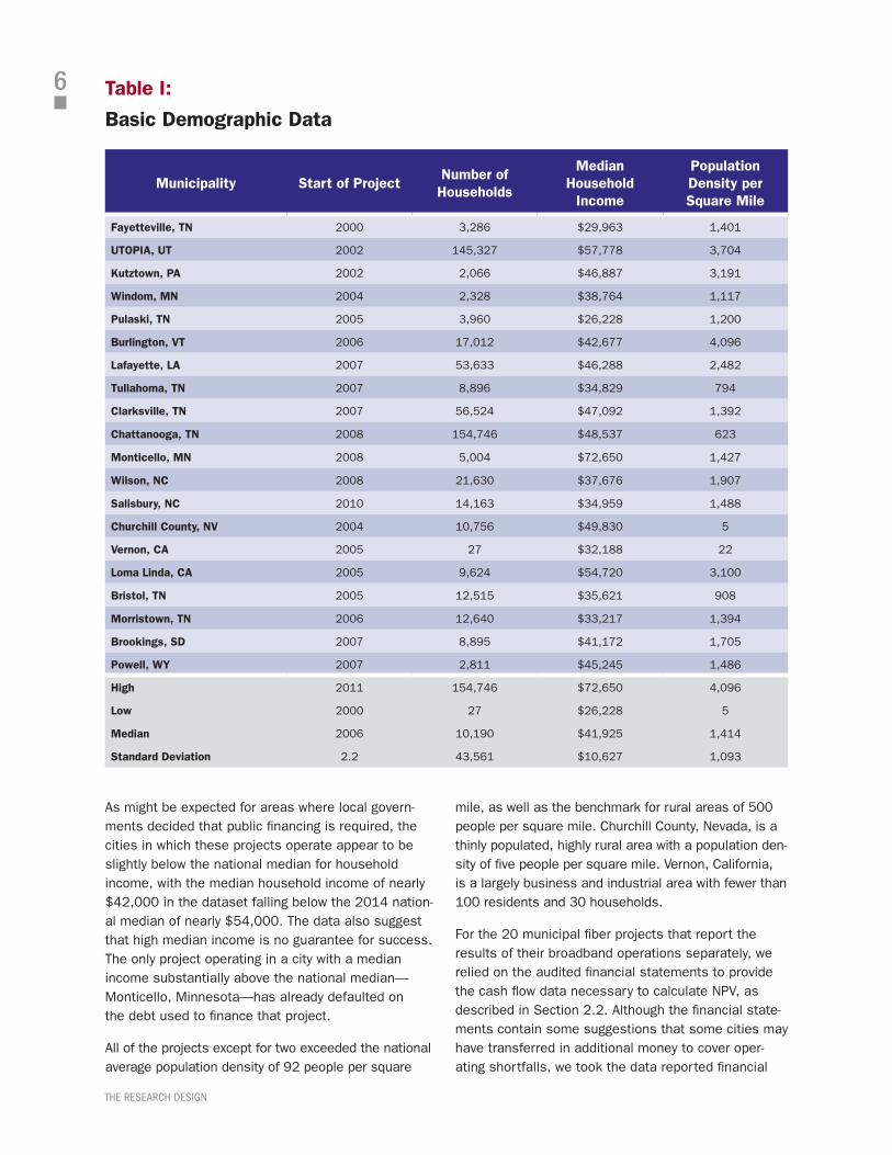
Basic demographic data about the 20 projects for which separate financial data exist appear in Table I. A project’s starting date and the number of households in the community provide key information about each project’s size and maturity, which in turn help place its financial results in perspective. The demographic data regarding median household income and population density (taken from the U.S. Census) shed light on the economic environment in which each project operates.

The projects range in age, with the oldest being 14 years old and the youngest being four years old as of 2014. The cities in which these projects operate vary widely in terms of size, with the smallest having only 27 households and the largest spanning nearly 155,000 households; the median community consists of 10,000 households.

11. The incentives to conceal poor financial results are demonstrated eloquently by the municipal fiber project in Bristol, Virginia, known as CPC OptiNet. It launched in 2004 in partnership with Bristol Virginia Utilities (BVU) and the Cumberland Plateau Company (CPC). OptiNet’s performance was obscured by the fact that BVU largely excluded OptiNet’s operations from its financial reports while simultaneously failing to issue separate financial statements for OptiNet. In 2009, BVU transitioned from municipal ownership to being an independent authority owned by the state in order make borrowing easier, which removed it from the oversight of the Bristol city council. Even though OptiNet has received $22.7 million in federal subsidies, $30.1 million in state subsidies, and $23.4 million in interfund transfers from BVU’s electric power operations and invested an additional $79.6 million generated through bond funding and operating cash flow, a state audit concluded that OptiNet does not have the resources to continue operating without receiving cross-subsidies from other operations that are prohibited by state law (Virginia APA 2016). OptiNet’s leadership has recently come under fire for improper management and conflicts of interest. In March 2017, OptiNet’s owners entered into a contract to sell its broadband operations to Sunset Digital for $50 million, which is essentially the amount of indebtedness remaining on the project without taking the subsidies into account.

6

THE RESEARCH DESIGN

As might be expected for areas where local govern-ments decided that public financing is required, the cities in which these projects operate appear to be slightly below the national median for household income, with the median household income of nearly $42,000 in the dataset falling below the 2014 nation-al median of nearly $54,000. The data also suggest that high median income is no guarantee for success. The only project operating in a city with a median income substantially above the national median—Monticello, Minnesota—has already defaulted on the debt used to finance that project.

All of the projects except for two exceeded the national average population density of 92 people per square

mile, as well as the benchmark for rural areas of 500 people per square mile. Churchill County, Nevada, is a thinly populated, highly rural area with a population den-sity of five people per square mile. Vernon, California, is a largely business and industrial area with fewer than 100 residents and 30 households.

For the 20 municipal fiber projects that report the results of their broadband operations separately, we relied on the audited financial statements to provide the cash flow data necessary to calculate NPV, as described in Section 2.2. Although the financial state-ments contain some suggestions that some cities may have transferred in additional money to cover oper-ating shortfalls, we took the data reported financial

Table I:

Basic Demographic Data

Municipality Start of ProjectNumber of Households

Median Household

Income

Population Density per Square Mile

Fayetteville, TN 2000 3,286 $29,963 1,401

UTOPIA, UT 2002 145,327 $57,778 3,704

Kutztown, PA 2002 2,066 $46,887 3,191

Windom, MN 2004 2,328 $38,764 1,117

Pulaski, TN 2005 3,960 $26,228 1,200

Burlington, VT 2006 17,012 $42,677 4,096

Lafayette, LA 2007 53,633 $46,288 2,482

Tullahoma, TN 2007 8,896 $34,829 794

Clarksville, TN 2007 56,524 $47,092 1,392

Chattanooga, TN 2008 154,746 $48,537 623

Monticello, MN 2008 5,004 $72,650 1,427

Wilson, NC 2008 21,630 $37,676 1,907

Salisbury, NC 2010 14,163 $34,959 1,488

Churchill County, NV 2004 10,756 $49,830 5

Vernon, CA 2005 27 $32,188 22

Loma Linda, CA 2005 9,624 $54,720 3,100

Bristol, TN 2005 12,515 $35,621 908

Morristown, TN 2006 12,640 $33,217 1,394

Brookings, SD 2007 8,895 $41,172 1,705

Powell, WY 2007 2,811 $45,245 1,486

High 2011 154,746 $72,650 4,096

Low 2000 27 $26,228 5

Median 2006 10,190 $41,925 1,414

Standard Deviation 2.2 43,561 $10,627 1,093

7

THE RESEARCH DESIGN

statements at face value without correcting for such transfers.

The two additional facts needed to assess NPV—project cost and weighted average cost of capital (WACC)—are taken from the official documents issued to underwrite the bonds used to finance each project, as reported to the Municipal Securities Rulemaking Board (MSRB). The project costs reflected in the bond documents may underestimate the actual capital costs for some of these projects. A review of media and industry reports suggests that many of these projects were supported by transfers or loans from a municipality’s electric power operations that are not reflected in the bond financing.

Table II:

Overview of Dataset

Number of Municipalities

Cash Flow

Project Cost

Cost of Capital

13 municipalities Actual Actual Actual

7 municipalities Actual Estimated Estimated

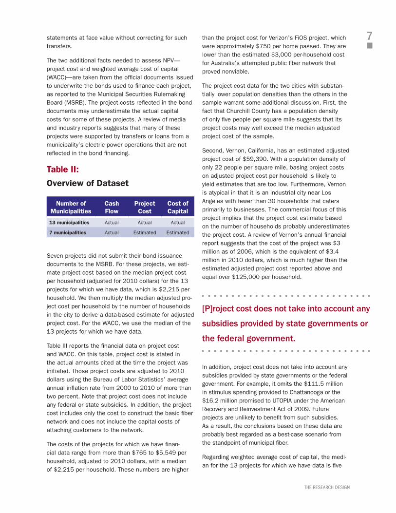
Seven projects did not submit their bond issuance documents to the MSRB. For these projects, we esti-mate project cost based on the median project cost per household (adjusted for 2010 dollars) for the 13 projects for which we have data, which is $2,215 per household. We then multiply the median adjusted pro-ject cost per household by the number of households in the city to derive a data-based estimate for adjusted project cost. For the WACC, we use the median of the 13 projects for which we have data.

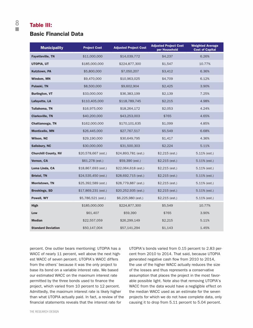
Table III reports the financial data on project cost and WACC. On this table, project cost is stated in the actual amounts cited at the time the project was initiated. Those project costs are adjusted to 2010 dollars using the Bureau of Labor Statistics’ average annual inflation rate from 2000 to 2010 of more than two percent. Note that project cost does not include any federal or state subsidies. In addition, the project cost includes only the cost to construct the basic fiber network and does not include the capital costs of attaching customers to the network.

The costs of the projects for which we have finan-cial data range from more than $765 to $5,549 per household, adjusted to 2010 dollars, with a median of $2,215 per household. These numbers are higher

than the project cost for Verizon’s FiOS project, which were approximately $750 per home passed. They are lower than the estimated $3,000 per-household cost for Australia’s attempted public fiber network that proved nonviable.

The project cost data for the two cities with substan-tially lower population densities than the others in the sample warrant some additional discussion. First, the fact that Churchill County has a population density of only five people per square mile suggests that its project costs may well exceed the median adjusted project cost of the sample.

Second, Vernon, California, has an estimated adjusted project cost of $59,390. With a population density of only 22 people per square mile, basing project costs on adjusted project cost per household is likely to yield estimates that are too low. Furthermore, Vernon is atypical in that it is an industrial city near Los Angeles with fewer than 30 households that caters primarily to businesses. The commercial focus of this project implies that the project cost estimate based on the number of households probably underestimates the project cost. A review of Vernon’s annual financial report suggests that the cost of the project was $3 million as of 2006, which is the equivalent of $3.4 million in 2010 dollars, which is much higher than the estimated adjusted project cost reported above and equal over $125,000 per household.

In addition, project cost does not take into account any subsidies provided by state governments or the federal government. For example, it omits the $111.5 million in stimulus spending provided to Chattanooga or the $16.2 million promised to UTOPIA under the American Recovery and Reinvestment Act of 2009. Future projects are unlikely to benefit from such subsidies. As a result, the conclusions based on these data are probably best regarded as a best-case scenario from the standpoint of municipal fiber.

Regarding weighted average cost of capital, the medi-an for the 13 projects for which we have data is five

[P]roject cost does not take into account any

subsidies provided by state governments or

the federal government.

8

THE RESEARCH DESIGN

percent. One outlier bears mentioning: UTOPIA has a WACC of nearly 11 percent, well above the next high-est WACC of seven percent. UTOPIA’s WACC differs from the others’ because it was the only project to base its bond on a variable interest rate. We based our estimated WACC on the maximum interest rate permitted by the three bonds used to finance the project, which varied from 10 percent to 12 percent. Admittedly, the maximum interest rate is likely higher than what UTOPIA actually paid. In fact, a review of the financial statements reveals that the interest rate for

UTOPIA’s bonds varied from 0.15 percent to 2.83 per-cent from 2010 to 2014. That said, because UTOPIA generated negative cash flow from 2010 to 2014, the use of the higher WACC actually reduces the size of the losses and thus represents a conservative assumption that places the project in the most favor-able possible light. Note also that removing UTOPIA’s WACC from the data would have a negligible effect on the median WACC used as an estimate for the seven projects for which we do not have complete data, only causing it to drop from 5.11 percent to 5.04 percent.

Table III:

Basic Financial Data

Municipality Project Cost Adjusted Project Cost Adjusted Project Cost

per HouseholdWeighted Average

Cost of Capital

Fayetteville, TN $11,000,000 $14,039,772 $4,237 6.26%

UTOPIA, UT $185,000,000 $224,877,300 $1,547 10.77%

Kutztown, PA $5,800,000 $7,050,207 $3,412 6.36%

Windom, MN $9,470,000 $10,963,025 $4,709 6.12%

Pulaski, TN $8,500,000 $9,602,904 $2,425 3.90%

Burlington, VT $33,000,000 $36,383,199 $2,139 7.25%

Lafayette, LA $110,405,000 $118,789,745 $2,215 4.98%

Tullahoma, TN $16,975,000 $18,264,172 $2,053 4.24%

Clarksville, TN $40,200,000 $43,253,003 $765 4.65%

Chattanooga, TN $162,000,000 $170,101,635 $1,099 4.85%

Monticello, MN $26,445,000 $27,767,517 $5,549 6.68%

Wilson, NC $29,190,000 $30,649,795 $1,417 4.36%

Salisbury, NC $30,000,000 $31,500,303 $2,224 5.11%

Churchill County, NV $20,578,667 (est.) $24,893,781 (est.) $2,215 (est.) 5.11% (est.)

Vernon, CA $61,278 (est.) $59,390 (est.) $2,215 (est.) 5.11% (est.)

Loma Linda, CA $18,867,693 (est.) $22,064,618 (est.) $2,215 (est.) 5.11% (est.)

Bristol, TN $24,535,450 (est.) $28,692,715 (est.) $2,215 (est.) 5.11% (est.)

Morristown, TN $25,392,589 (est.) $28,779,887 (est.) $2,215 (est.) 5.11% (est.)

Brookings, SD $17,869,231 (est.) $20,252,935 (est.) $2,215 (est.) 5.11% (est.)

Powell, WY $5,786,521 (est.) $6,225,980 (est.) $2,215 (est.) 5.11% (est.)

High $185,000,000 $224,877,300 $5,549 10.77%

Low $61,407 $59,390 $765 3.90%

Median $22,557,059 $26,299,149 $2,215 5.11%

Standard Deviation $50,147,004 $57,141,294 $1,143 1.45%

9

THE RESEARCH DESIGN

2.2 Five-Year Net Present Value (NPV)The data from the official bond documents can be combined with the data from the audited financial statements submitted by these projects to calculate the primary financial tool used by the investment com-munity for valuing projects: Net Present Value (NPV). NPV reflects that the fact the income statements typically provide a misleading perception of an ongo-ing operation’s viability. Instead of basing its analysis on the accounting profits and losses reported on the income statement, NPV focuses on the cash flowing into and out of an organization. Cash flow is generally regarded as more relevant because it (and not income) determines whether an organization becomes insolvent and must either raise more capital or default. The crit-ical importance of cash flow explains why all financial statements include statements of cash flow along with balance sheets and income statements and why cred-itors place the most emphasis on projected cash flows.

We then calculate cash flow for each project for the five years beginning in 2010 and ending in 2014. The stan-dard method for calculating net cash flow in financial statements requires adding noncash operating expens-es back to operating income to determine the impact of a particular year’s operations on each municipality’s cash position. Noncash adjustments can be significant, sometimes causing a given year’s cash flow to deviate from its reported income by millions of dollars.

The most significant noncash expense is deprecia-tion, which is the method for allocating the costs of long-lived capital investments across multiple years. Consider a project that requires an up-front invest-ment of $30 million for equipment that is expected to last 30 years. On income statements, the cost of that investment is allocated across the expected useful life of the project, which under straight-line depreciation would be $1 million per year. The impact of this invest-ment on the project’s cash position is much different. The project would have to make the entire $30 million payment in year zero and no additional payments in any later years. This means that the income statement will overstate the project’s financial performance in year zero and understate the project’s financial perfor-mance in all later years.

Income statements also exclude non-operating cash ex-penses, such as “capital and related financing,” which includes payments to cover financing obligations as well the cost to acquire any additional capital that may have become necessary. These amounts must also be taken into account when determining cash flow even

though they will not appear on the income statement. Note that this analysis does not take into account interfund transfers from a municipality’s electricity operations or from other forms of non capital financing used to support either FTTH operation. Indeed, there is evidence that some municipalities may have made some transfers to balance their books in particular years. The systematic, city-specific examination that would be required to determine whether shortfalls in FTTH operations were being covered by transfers from other accounts would have caused so much deviation from the data as reported that we opted to rely on the data from the financial statements without identifying and correcting for these transfers.

Note also that bonds are sometimes structured to re-quire minimal capital repayments during most of their life and to make a large balloon payment towards the end of the bond period. Balloon payments are appropriate for projects with long useful lives that are likely to be refinanced by additional bonds. The fact that broadband networks are assumed to have useful lives of 30 to 40 years raises questions about using such a repayment structure for a municipal fiber proj-ect. In any event, the use of large balloon payments towards the end of the project means that the cash flow data from 2010 to 2014 do not include their fair share of capital service. As such, they arguably por-tray an optimistic picture of these projects’ financial prospects.

The cash flow for any particular year also properly includes any increases or decreases in net working capital required by operations, which is the change in the project’s current assets and current liabilities. This adjustment accounts for increases in noncash current assets, such as accounts receivable, which are reported as revenue on the income statement but are not immediately realized as cash. Similarly, this adjustment also accounts for increases in current lia-bilities, such as accounts payable, which are reported as an expense on the income statement but are not immediately paid out in cash. Changes in working capital can be quite significant.

Lastly, future cash flows are generally worth less than current cash flows. The real impact of a $1 million expense is less than $1 million if it can be delayed by a year, because the money can be invested during that year and earn interest or, if the organization is already in debt, can reduce the principal on which the project must pay interest during that year. Conversely, $1 million in receipts is worth less if postponed a year,

10

THE RESEARCH DESIGN

Figure 1:

Expected Cash Flow Pattern for an Investment

Positve cash flow (in)

Negative cash flows (out)

1

F1

F2

2 3 4 5 6 n

F3

F4

F5

F6

Fn

................................

0

FO

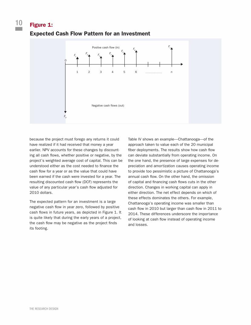
because the project must forego any returns it could have realized if it had received that money a year earlier. NPV accounts for these changes by discount-ing all cash flows, whether positive or negative, by the project’s weighted average cost of capital. This can be understood either as the cost needed to finance the cash flow for a year or as the value that could have been earned if the cash were invested for a year. The resulting discounted cash flow (DCF) represents the value of any particular year’s cash flow adjusted for 2010 dollars.

The expected pattern for an investment is a large negative cash flow in year zero, followed by positive cash flows in future years, as depicted in Figure 1. It is quite likely that during the early years of a project, the cash flow may be negative as the project finds its footing.

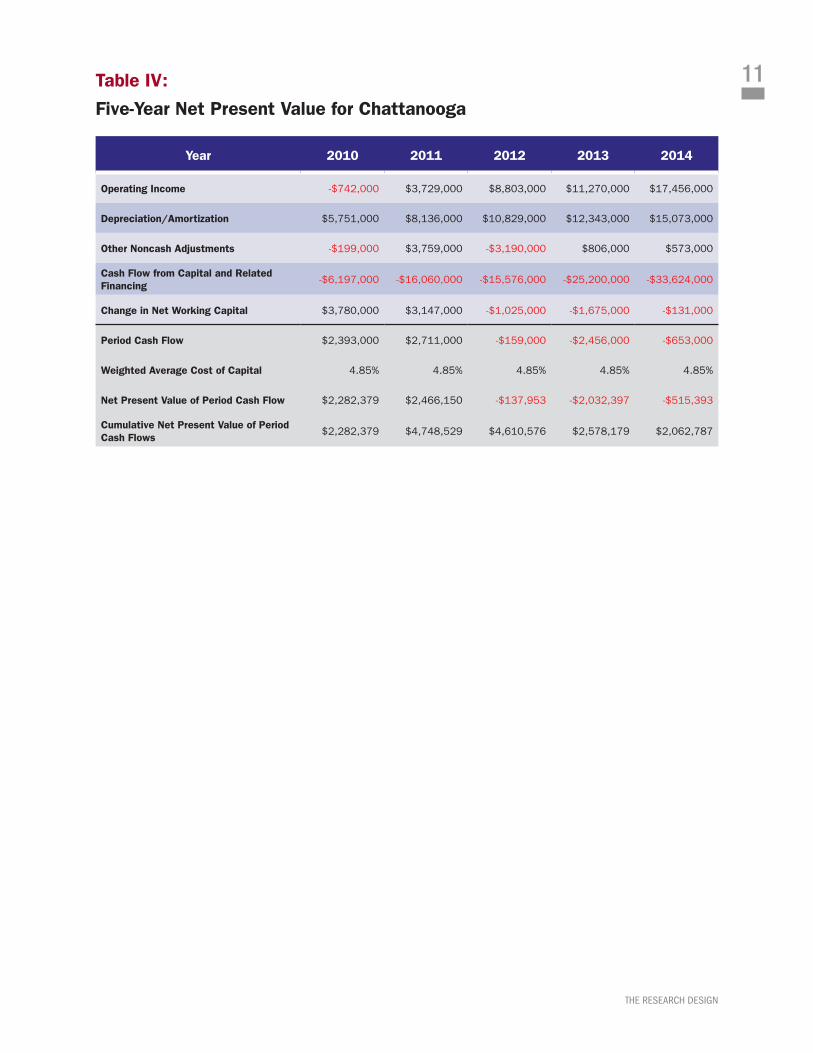
Table IV shows an example—Chattanooga—of the approach taken to value each of the 20 municipal fiber deployments. The results show how cash flow can deviate substantially from operating income. On the one hand, the presence of large expenses for de-preciation and amortization causes operating income to provide too pessimistic a picture of Chattanooga’s annual cash flow. On the other hand, the omission of capital and financing cash flows cuts in the other direction. Changes in working capital can apply in either direction. The net effect depends on which of these effects dominates the others. For example, Chattanooga’s operating income was smaller than cash flow in 2010 but larger than cash flow in 2011 to 2014. These differences underscore the importance of looking at cash flow instead of operating income and losses.

11

THE RESEARCH DESIGN

Table IV:

Five-Year Net Present Value for Chattanooga

Year 2010 2011 2012 2013 2014

Operating Income -$742,000 $3,729,000 $8,803,000 $11,270,000 $17,456,000

Depreciation/Amortization $5,751,000 $8,136,000 $10,829,000 $12,343,000 $15,073,000

Other Noncash Adjustments -$199,000 $3,759,000 -$3,190,000 $806,000 $573,000

Cash Flow from Capital and Related Financing

-$6,197,000 -$16,060,000 -$15,576,000 -$25,200,000 -$33,624,000

Change in Net Working Capital $3,780,000 $3,147,000 -$1,025,000 -$1,675,000 -$131,000

Period Cash Flow $2,393,000 $2,711,000 -$159,000 -$2,456,000 -$653,000

Weighted Average Cost of Capital 4.85% 4.85% 4.85% 4.85% 4.85%

Net Present Value of Period Cash Flow $2,282,379 $2,466,150 -$137,953 -$2,032,397 -$515,393

Cumulative Net Present Value of Period Cash Flows

$2,282,379 $4,748,529 $4,610,576 $2,578,179 $2,062,787

12

THE EMPIRICAL RESULTS

3. THE EMPIRICAL RESULTSWe replicate the five-year NPV calculation conducted on the financial data from Chattanooga for all of the projects encompassed in our study. The results for 19 projects include the period beginning in 2010 and ending in 2014. One project (Vernon, California) did not begin reporting its fiber operations separately until 2011 and thus yields only four years of data. NPV provides the standard tool for analyzing a project’s financial success.

3.1 Assessing Each Project’s Potential for Success

We compare each project’s five-year NPV to its project cost to evaluate the likelihood that the project will re-main solvent. To correct for differences in project age, we adjust all project costs to the equivalent of 2010 dollars. As noted earlier, project cost does not include any state or federal subsidies.

If a project’s five-year NPV is negative, the fact that ongoing operations are creating cash losses raises serious questions about whether the project should continue to operate. If a project’s five-year NPV is positive, its likelihood of breaking even depends on whether the positive cash flow is large enough to cover the project cost. To provide some sense of the likelihood, we calculate the number of years a project would take to recover its project costs if it were to continue to generate cash at the rates generated from 2010 to 2014. We also report the age of the project and the current rate of revenue growth to provide per-spective about the likelihood that a project’s financial condition might sufficiently improve in future years to make the project financially viable. The growth rates for extremely young projects are expected to be very high, as the denominator for any growth calculation is likely to be quite small. Growth rates can be expected to taper off as a project matures.

Even before taking into account project cost, a key finding is that 11 of the 20 projects are cash-flow negative, many of them substantially so. The modest revenue growth rates for most of these cities offers lit-tle promise that their operations are likely to improve enough to become cash-flow positive, let alone cover project costs. Of those with the highest growth rates,

one (Monticello, Minnesota) has already defaulted on its bonds and another (Salisbury, North Carolina) has had its bond rating cut out of concern that a default may be imminent.

For projects that are cash-flow positive, the key ques-tion is whether the cash flows are sufficiently large to support recovery of project costs. A rough estimate of how quickly municipal fiber projects can expect to cov-er their project costs is the number of years it would take the projects in our data set to recover its initial project costs if operating cash flow remained at 2010 to 2014 levels. For reference, financial statements often estimate that fiber networks will have a useful life of 30 to 40 years.

Of the nine projects in our dataset that are cash-flow positive, five have cash flow that is so small that recovering project costs would take more than a century (Pulaski, Tennessee; Tullahoma, Tennessee; Chattanooga, Tennessee; Powell, Wyoming; Brookings, South Dakota). Again, the relatively modest annu-al growth rates raise serious questions about how much these projects’ financial performance is likely to improve. For two other municipalities (Fayetteville, Tennessee; Windom, Minnesota), the recovery period is 61 and 65 years, beyond the 30- to 40-year expect-ed useful life of a fiber network.

The data identify only two potential success stories. First, at 34 years, Bristol, Tennessee, is on track to recover its project costs within a reasonable life expectancy of the fiber network.12 Second, Vernon gen-erated enough cash flow from 2011 to 2014 to cover its estimated adjusted project costs. As noted earlier, Vernon’s municipal fiber project is atypical in ways

For projects that are cash-flow positive,

the key question is whether the cash flows

are sufficiently large to support recovery of

project costs.

12. Note that Bristol, Tennessee, refers to the project in Tennessee operated by Bristol Tennessee Essential Services (BTES), not the project in Bristol, Virginia, operated by Bristol Virginia Utilities (BVU) that was recently sold to a private company.

13

THE EMPIRICAL RESULTS

that may understate its project costs, and the city’s commercially oriented nature limits its usefulness as a role model for other cities. If we use the adjusted project cost of $3.4 million derived from Vernon’s 2006 financial statements, the payback period length-ens to 110 years.

3.2 Modeling the Returns for a Hypothetical Project

The data permit us to estimate how a hypothetical project might perform. We approach this in two ways.

First, we use the actual returns achieved by these cities to estimate how a future project might perform during the 14-year period for which we have data. Second, we conduct regression analysis on the data to construct a model that allows us to project the financial performance of a hypothetical project into the future.

Beginning first with the model based on actual returns, the data include projects of a wide range of ages. Some of the projects were newly formed, with one starting the year after the study period began. The oldest had been operating for 10 years as of 2010 and for 14

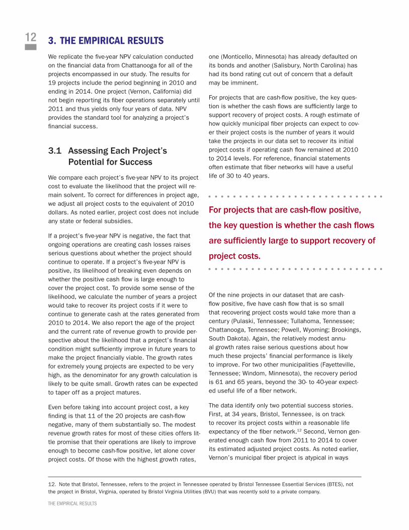
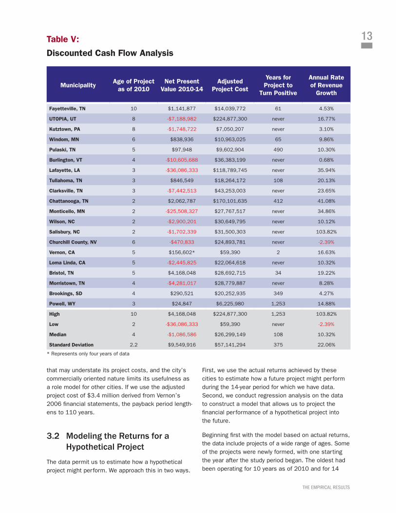
Table V:

Discounted Cash Flow Analysis

MunicipalityAge of Project

as of 2010Net Present

Value 2010-14Adjusted

Project Cost

Years for Project to

Turn Positive

Annual Rate of Revenue

Growth

Fayetteville, TN 10 $1,141,877 $14,039,772 61 4.53%

UTOPIA, UT 8 -$7,188,982 $224,877,300 never 16.77%

Kutztown, PA 8 -$1,748,722 $7,050,207 never 3.10%

Windom, MN 6 $838,936 $10,963,025 65 9.86%

Pulaski, TN 5 $97,948 $9,602,904 490 10.30%

Burlington, VT 4 -$10,605,688 $36,383,199 never 0.68%

Lafayette, LA 3 -$36,086,333 $118,789,745 never 35.94%

Tullahoma, TN 3 $846,549 $18,264,172 108 20.13%

Clarksville, TN 3 -$7,442,513 $43,253,003 never 23.65%

Chattanooga, TN 2 $2,062,787 $170,101,635 412 41.08%

Monticello, MN 2 -$25,508,327 $27,767,517 never 34.86%

Wilson, NC 2 -$2,900,201 $30,649,795 never 10.12%

Salisbury, NC 2 -$1,702,339 $31,500,303 never 103.82%

Churchill County, NV 6 -$470,833 $24,893,781 never -2.39%

Vernon, CA 5 $156,602* $59,390 2 16.63%

Loma Linda, CA 5 -$2,445,825 $22,064,618 never 10.32%

Bristol, TN 5 $4,168,048 $28,692,715 34 19.22%

Morristown, TN 4 -$4,281,017 $28,779,887 never 8.28%

Brookings, SD 4 $290,521 $20,252,935 349 4.27%

Powell, WY 3 $24,847 $6,225,980 1,253 14.88%

High 10 $4,168,048 $224,877,300 1,253 103.82%

Low 2 -$36,086,333 $59,390 never -2.39%

Median 4 -$1,086,586 $26,299,149 108 10.32%

Standard Deviation 2.2 $9,549,916 $57,141,294 375 22.06%

* Represents only four years of data

14

THE EMPIRICAL RESULTS

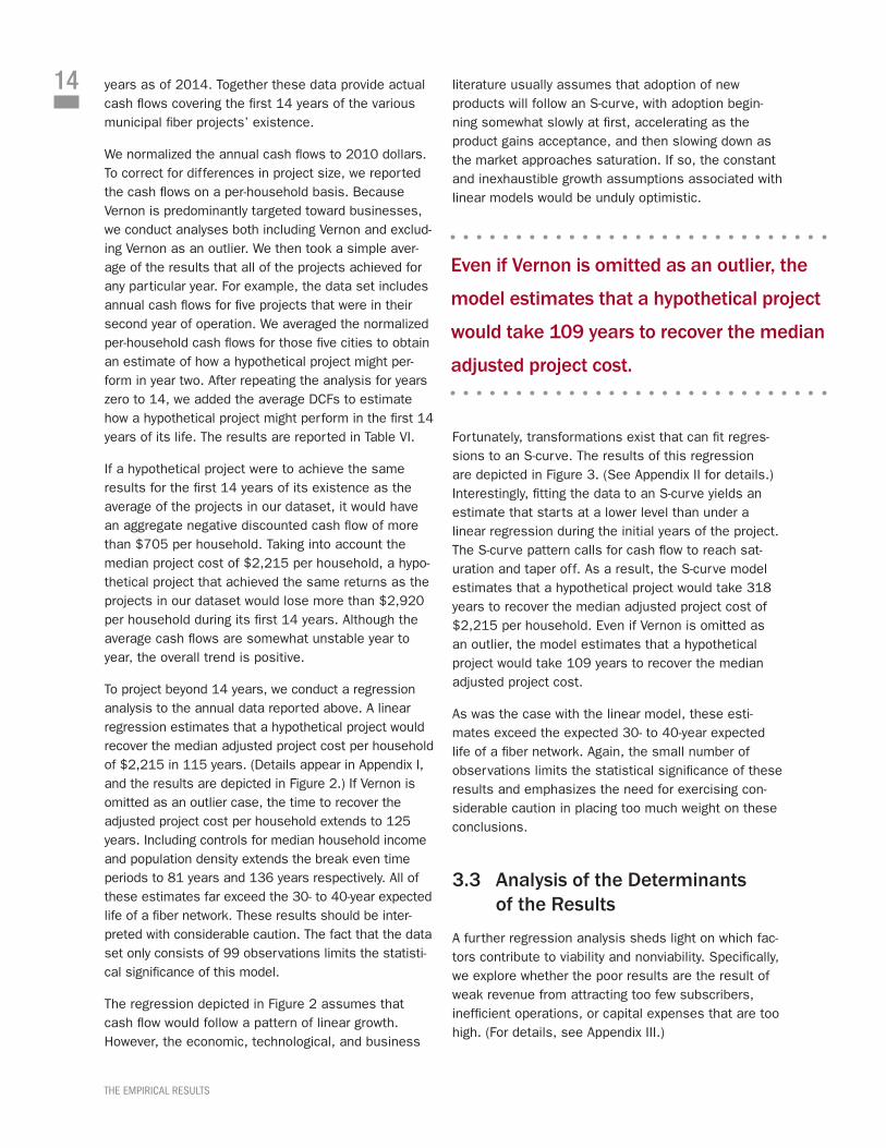
years as of 2014. Together these data provide actual cash flows covering the first 14 years of the various municipal fiber projects’ existence.

We normalized the annual cash flows to 2010 dollars. To correct for differences in project size, we reported the cash flows on a per-household basis. Because Vernon is predominantly targeted toward businesses, we conduct analyses both including Vernon and exclud-ing Vernon as an outlier. We then took a simple aver-age of the results that all of the projects achieved for any particular year. For example, the data set includes annual cash flows for five projects that were in their second year of operation. We averaged the normalized per-household cash flows for those five cities to obtain an estimate of how a hypothetical project might per-form in year two. After repeating the analysis for years zero to 14, we added the average DCFs to estimate how a hypothetical project might perform in the first 14 years of its life. The results are reported in Table VI.

If a hypothetical project were to achieve the same results for the first 14 years of its existence as the average of the projects in our dataset, it would have an aggregate negative discounted cash flow of more than $705 per household. Taking into account the median project cost of $2,215 per household, a hypo-thetical project that achieved the same returns as the projects in our dataset would lose more than $2,920 per household during its first 14 years. Although the average cash flows are somewhat unstable year to year, the overall trend is positive.

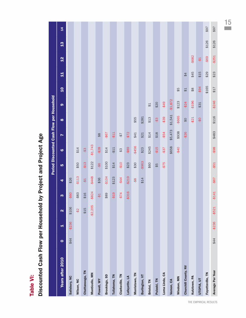
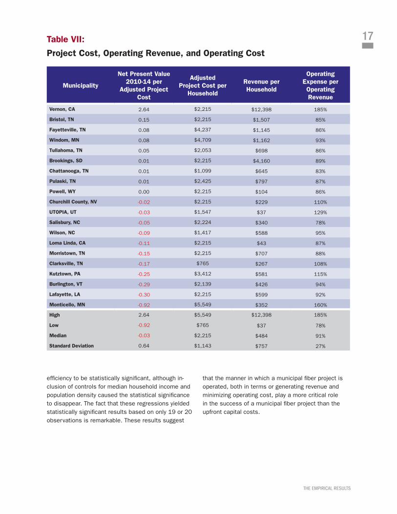
To project beyond 14 years, we conduct a regression analysis to the annual data reported above. A linear regression estimates that a hypothetical project would recover the median adjusted project cost per household of $2,215 in 115 years. (Details appear in Appendix I, and the results are depicted in Figure 2.) If Vernon is omitted as an outlier case, the time to recover the adjusted project cost per household extends to 125 years. Including controls for median household income and population density extends the break even time periods to 81 years and 136 years respectively. All of these estimates far exceed the 30- to 40-year expected life of a fiber network. These results should be inter-preted with considerable caution. The fact that the data set only consists of 99 observations limits the statisti-cal significance of this model.

The regression depicted in Figure 2 assumes that cash flow would follow a pattern of linear growth. However, the economic, technological, and business

literature usually assumes that adoption of new products will follow an S-curve, with adoption begin-ning somewhat slowly at first, accelerating as the product gains acceptance, and then slowing down as the market approaches saturation. If so, the constant and inexhaustible growth assumptions associated with linear models would be unduly optimistic.

Fortunately, transformations exist that can fit regres-sions to an S-curve. The results of this regression are depicted in Figure 3. (See Appendix II for details.) Interestingly, fitting the data to an S-curve yields an estimate that starts at a lower level than under a linear regression during the initial years of the project. The S-curve pattern calls for cash flow to reach sat-uration and taper off. As a result, the S-curve model estimates that a hypothetical project would take 318 years to recover the median adjusted project cost of $2,215 per household. Even if Vernon is omitted as an outlier, the model estimates that a hypothetical project would take 109 years to recover the median adjusted project cost.

As was the case with the linear model, these esti-mates exceed the expected 30- to 40-year expected life of a fiber network. Again, the small number of observations limits the statistical significance of these results and emphasizes the need for exercising con-siderable caution in placing too much weight on these conclusions.

3.3 Analysis of the Determinants of the Results

A further regression analysis sheds light on which fac-tors contribute to viability and nonviability. Specifically, we explore whether the poor results are the result of weak revenue from attracting too few subscribers, inefficient operations, or capital expenses that are too high. (For details, see Appendix III.)

Even if Vernon is omitted as an outlier, the

model estimates that a hypothetical project

would take 109 years to recover the median

adjusted project cost.

15

THE EMPIRICAL RESULTS

Tabl

e V

I:

Dis

coun

ted

Cas

h Fl

ow p

er H

ouse

hold

by

Pro

ject

and

Pro

ject

Age

Per

iod

Dis

coun

ted

Cas

h Fl

ow p

er H

ouse

hold

Year

s af

ter

2010

01

23

45

67

89

10

11

12

13

14

Sal

isbu

ry,

NC

$4

4-$

23

6$106

-$60

$26

Wils

on,

NC

-$2

-$83

-$113

$50

$14

Cha

ttan

ooga

, TN

$15

$16

-$1

-$13

-$3

Mon

tice

llo,

MN

-$2,2

05

-$824

-$448

$122

-$1,7

43

Pow

ell,

WY

-$1

$36

-$6

-$28

$8

Bro

okin

gs,

SD

$89

-$104

$100

$14

-$67

Tulla

hom

a, T

N-$

19

$123

$14

-$11

-$11

Cla

rksv

ille,

TN

-$74

-$44

-$10

$3

-$7

Lafa

yett

e, L

A-$

316

-$219

$23

-$89

-$72

Mor

rist

own,

TN

-$8

$30

-$456

$41

$55

Bur

lingt

on,

VT

$14

-$963

$23

$21

$281

Bri

stol

, TN

$60

$245

$14

$13

$1

Pul

aski

, TN

$5

-$15

$18

-$3

$20

Lom

a Li

nda,

CA

-$75

-$37

-$54

-$39

-$49

Vern

on,

CA

$658

$5,4

73

$1,5

41

-$1,8

72

Win

dom

, M

N-$

40

$938

-$665

$123

$5

Chu

rchi

ll C

ount

y, N

V-$

26

$0

-$24

$1

$4

Kut

ztow

n, P

A-$

21

-$196

$8

$45

-$682

UTO

PIA

, U

T-$

0$31

-$94

$15

-$1

Faye

ttev

ille,

TN

$165

$29

-$69

$126

$97

Ave

rage

Per

Yea

r$

44

-$2

36

-$521

-$141

-$67

-$51

-$98

$483

$116

-$246

$17

$23

-$251

$126

$97

16

THE EMPIRICAL RESULTS

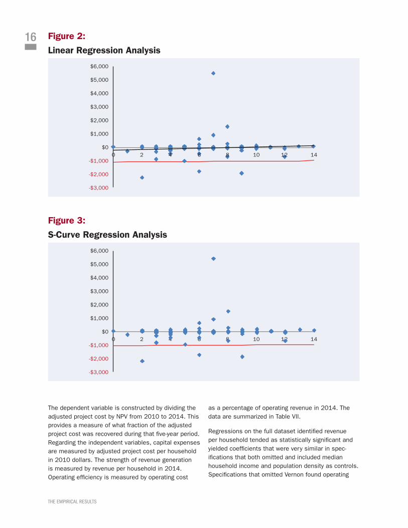
The dependent variable is constructed by dividing the adjusted project cost by NPV from 2010 to 2014. This provides a measure of what fraction of the adjusted project cost was recovered during that five-year period. Regarding the independent variables, capital expenses are measured by adjusted project cost per household in 2010 dollars. The strength of revenue generation is measured by revenue per household in 2014. Operating efficiency is measured by operating cost

as a percentage of operating revenue in 2014. The data are summarized in Table VII.

Regressions on the full dataset identified revenue per household tended as statistically significant and yielded coefficients that were very similar in spec-ifications that both omitted and included median household income and population density as controls. Specifications that omitted Vernon found operating

Figure 3:

S-Curve Regression Analysis

0 2 4 6 8 10 12 14

$6,000

$5,000

$4,000

$3,000

$2,000

$1,000

$0

-$1,000

-$2,000

-$3,000

Figure 2:

Linear Regression Analysis

0 2 4 6 8 10 12 14

$6,000

$5,000

$4,000

$3,000

$2,000

$1,000

$0

-$1,000

-$2,000

-$3,000

17

THE EMPIRICAL RESULTS

Table VII:

Project Cost, Operating Revenue, and Operating Cost

Municipality

Net Present Value 2010-14 per

Adjusted Project Cost

Adjusted Project Cost per

Household

Revenue per Household

Operating Expense per Operating Revenue

Vernon, CA 2.64 $2,215 $12,398 185%

Bristol, TN 0.15 $2,215 $1,507 85%

Fayetteville, TN 0.08 $4,237 $1,145 86%

Windom, MN 0.08 $4,709 $1,162 93%

Tullahoma, TN 0.05 $2,053 $698 86%

Brookings, SD 0.01 $2,215 $4,160 89%

Chattanooga, TN 0.01 $1,099 $645 83%

Pulaski, TN 0.01 $2,425 $797 87%

Powell, WY 0.00 $2,215 $104 86%

Churchill County, NV -0.02 $2,215 $229 110%

UTOPIA, UT -0.03 $1,547 $37 129%

Salisbury, NC -0.05 $2,224 $340 78%

Wilson, NC -0.09 $1,417 $588 95%

Loma Linda, CA -0.11 $2,215 $43 87%

Morristown, TN -0.15 $2,215 $707 88%

Clarksville, TN -0.17 $765 $267 108%

Kutztown, PA -0.25 $3,412 $581 115%

Burlington, VT -0.29 $2,139 $426 94%

Lafayette, LA -0.30 $2,215 $599 92%

Monticello, MN -0.92 $5,549 $352 160%

High 2.64 $5,549 $12,398 185%

Low -0.92 $765 $37 78%

Median -0.03 $2,215 $484 91%

Standard Deviation 0.64 $1,143 $757 27%

efficiency to be statistically significant, although in-clusion of controls for median household income and population density caused the statistical significance to disappear. The fact that these regressions yielded statistically significant results based on only 19 or 20 observations is remarkable. These results suggest

that the manner in which a municipal fiber project is operated, both in terms or generating revenue and minimizing operating cost, play a more critical role in the success of a municipal fiber project than the upfront capital costs.

18

CASE STUDIES

4. CASE STUDIESThe overall data paint a relatively pessimistic picture of municipal fiber projects’ financial prospects. Of the 20 projects, more than half are cash-flow nega-tive, and 18 were unable to generate sufficient cash between 2010 and 2014 to recover their project costs within the life expectancy of the broadband network.

That said, insight can be gained by conducting case studies of specific projects to see the causes of suc-cess and failure. This section begins by focusing on the potential success stories: Bristol, Tennessee, and Vernon, California.

This section also examines a number of other projects that have garnered significant attention from industry analysts, policy advocates, and the media, starting with Chattanooga and proceeding to the others in the order of their date of inception. Media attention is ad-mittedly a nonobjective basis for selecting case stud-ies, but if anything, the bias is toward those projects that are regarded as the most promising. Moreover, like the underlying data set, these case studies do not include municipal fiber projects that have already been liquidated, such as Provo, Utah, which was sold to Google for $1 and still left the city holding $39 million in debt; Dunnellon, Florida, which was sold for $1 mil-lion and left behind $7 million in debt after losing as much as $300,000 per month; and Marietta, Georgia, which sold its $30 million fiber network at a loss of $11 million.

On the other hand, the case studies omit a number of projects that have garnered little media attention but are sufficiently cash-flow positive to have an outside chance of breaking even. Specifically, these include Fayetteville, Tennessee, and Windom, Minnesota, which would recover their project costs in less than 70 years at the cash-flow rates achieved from 2010 to 2014. Unfortunately, there is insufficient secondary material to develop full case studies around these projects.

4.1 Bristol, TennesseeOf all the projects in this study, the project operated by Bristol Tennessee Essential Services (BTES) appears to be the only one with a reasonable prospect of recov-ering its costs. BTES began providing telephone and Internet service via DSL in 2005 and began offering gigabit service via a fiber network in 2012.

If BTES continues to generate cash flow at the rate it achieved from 2010 to 2014, it would pay off its estimated project cost in 34 years. The pattern of the cash flows do raise some cause for concern. Although the project is cash-flow positive over the entire five-year period running from 2010 to 2014, the magnitude of the cash flows decreased during the last three years of the study, dropping from a high of $245 per household in 2011 to a mere $1 per household in 2014. This is a particular concern because BTES did not begin offering fiber until 2012. The strong 2010 and 2011 results thus reflect the success of BTES’s DSL operations, although BTES undoubtedly incurred capital costs in 2010 and 2011. While BTES contin-ued to be cash-flow positive in 2012–2014, the overall performance from 2010–2014 likely overstates its chances to break even. If the analysis is restricted to the cash-flow rates from 2012–2014, the break even period lengthens to over 200 years. The project is relatively young, and revenue grew at a robust rate of more than 19 percent from 2010 to 2014; that time period covered years five to nine of the project’s over-all operations. This suggests that its cash flow has some upside room to grow.

The data reveal the reasons for BTES’s success. BTES’s revenue of more than $1,500 per house-hold exceeds the dataset average of nearly $450 per household reflected in the overall data set and ranks third among the projects we studied. BTES also appears to be operating efficiently, with costs amount-ing to 85 percent of revenue. Note that we estimated BTES’s project cost at $24.5 million based on the median cost per household in our data set. BTES’s financial statements reflect the more modest amount of $14.8 million in capital assets in its Advanced Broadband Services Business Unit.

Somewhat surprisingly, BTES has garnered relative-ly little publicity despite its strong performance. In 2010, city leaders began a drive to use fiber to attract new businesses in an attempt to capture some of the acclaim being garnered by Chattanooga.

4.2 Vernon, CaliforniaOn paper, the municipal fiber project initiated by Vernon appears to possess the best financial picture in our data set. The project only began reporting its broadband operations separately in 2011, so the

19

CASE STUDIES

data cover only four years. Between 2011 and 2014, Vernon averaged a DCF of more than $38,000 per year for a four-year total of $156,602. The fact that the estimated project cost was less than $60,000, measured in 2010 dollars, suggests that Vernon should have been able to recoup its investment in less than two years. A review of Vernon’s annual finan-cial statements suggests that the project costs were substantially higher, equalling $3 million as of 2006, in which case the payback period lengthens to over 100 years.

A closer look raises further questions about whether Vernon can serve as a model for other cities. Vernon is the smallest incorporated city in California, covering only 5.2 square miles. It is an industrial city just south of downtown Los Angeles with only 30 homes and 100 residents, compared with the 1,800 businesses and 55,000 people employed there. That explains why its population density of 22 people per square mile is so much lower than that of the other cities in this study. The fact that the network was constructed for busi-nesses and not residents suggests why the estimate based on the number of households appears to under-state the true project cost. It also explains why Vernon was able to generate revenue per household that is 24 times higher than the overall rates generated by the projects in this study.

In addition, the financial results raise some cause for concern. As an initial matter, Vernon’s municipal fiber project consistently runs annual operating losses of roughly $275,000, although these paper losses are largely the product of large depreciation and other noncash adjustments that do not affect cash flow. At the same time, the cash flow in 2014 was negative after running positive from 2011 to 2013. In addition, revenue grew only at an annual rate of almost 17 per-cent. Such a low growth rate does not augur well for a young project.

Of even greater concern are the problems identified in a 2011 investigative report published by the Los Angeles Times (Becerra 2011). The paper reported that Vernon’s electric utility amassed nearly half a billion dollars in debt through a series of increasingly complex and grandiose investments, as well as exces-sive spending on employee compensation and fees for lawyers and consultants. Although the article conclud-ed that Vernon is unlikely to default on its obligations, its bond rating is relatively low compared with its

peers. The city also raised electric power rates 16 per-cent in 2011 and announced plans to increase rates five percent each year for the next decade after that. Vernon’s atypical nature is further underscored by the fact that Vernon pays its city leaders and outside legal counsel far more than the average city. Allegations of public corruption have also led the California State Assembly to consider legislation to force Vernon to disincorporate.

Vernon’s unusual demographic characteristics make project cost difficult to estimate and make it problem-atic as a model for other cities to follow. In addition, the troubled state of the electric power utility raises plenty of reasons for caution.

4.3 Chattanooga, TennesseeOf all the projects in this study, the project in Chattanooga is by far the best known. Key pol-icymakers, such as the OECD and the Federal Communications Commission, and media thought leaders, such as the New York Times and the Washington Post, repeatedly point to Chattanooga as a model for others to emulate. Chattanooga now pro-motes itself as “Gig City” and claims to have attracted new businesses and jobs to the area. Chattanooga has actively advocated for expanding municipal fiber, having successfully petitioned the FCC in February 2015 to preempt state laws barring municipal broad-band; that decision was appealed and overturned by the courts in August 2016.

Although associated most strongly with Chattanooga, the project also includes other nearby cities.13 It is run by the Electric Power Board of Chattanooga (EPB), which also serves as the electric power utility for the area. The EPB board approved the plan to offer FTTH service in 2007, and Chattanooga granted EPB a fran-chise to do so in 2008. Initial planning was financed by a $50 million loan from EPB’s electric power oper-ations. Construction was financed by $220 million in local revenue bonds, $162 million of which were used to fund the fiber project. The project also received $111.5 million in federal stimulus funding from the U.S. Department of Energy to promote the deploy-ment of smart grids. The project cost in this analysis considers only the $162 million of bond revenue and omits the $50 million EPB loan and $111.5 million in stimulus funding.

13. The Chattanooga project also provides service to Red Bank, East Ridge, Ridgeside, Hamilton County, Signal Mountain, Soddy Daisy, and Rossville in Tennessee and Lookout Mountain in Georgia.

20

CASE STUDIES

EPB began offering broadband service in 2009 and has achieved strong penetration. It generated more than $1,200 per household in 2014, compared with the average of $446 generated overall by the projects in this study. Lower-speed subscriptions accumulated, although the high prices (more than $350 per month) slowed adoption of gigabit service. The Economist (2012) reported that EPB had only nine residents and two business that had subscribed to the $350 gigabit service two years into the project. EPB subsequently dropped prices to more competitive levels and now is enjoying more robust subscribership for gigabit service.

EPB’s fiber operations were cash-flow positive by roughly $2 million from 2010 to 2014. While repaying the project cost would take 412 years at this rate, the project is relatively young, and revenue grew at a healthy 41 percent annual rate from 2010 to 2014.

A closer look at EPB’s financial returns does raise some concerns about EPB’s future. EPB’s fiber oper-ations did generate over $2 million in positive cash flow during the five-year period from 2010 to 2014. Unfortunately, this number is dwarfed by the $162 million in bond indebtedness that EPB undertook to finance this venture. In addition, an examination of the annual cash flows from 2010 to 2014 reveals that although cash flow was positive for 2010 and 2011 and for the entire five-year period, it was negative in 2012, 2013, and 2014. The instability of cash flows caused by major financing deadlines makes it difficult to determine whether this represents a broader trend that is likely to continue. Moreover, the Chattanooga bond requires a $71.7 million principal payment in 2033, which represents 44% of the total indebted-ness. Backloading the repayment of principal is quite common. It envisions that the bond will be refinanced with another a new issuance. That said, because the cash flows from 2010 to 2014 do not include a proportionate share of the repayments of principal, if anything these data understate the difficulties that Chattanooga may face in covering its project costs.

A final note of caution comes from the fact that EPB achieved these returns with the support of $111.5 million in stimulus funding that future projects are unlikely to be able to duplicate. Including the stimulus money in the project cost would increase the time

needed for the project to break even from 412 years to 683 years, assuming that cash flow remains at the rates realized during the period from 2010 to 2014.

The 2007 EPB proposal that supported the Chattanooga project was based in part on the as-sumption that the fiber optic network would provide sufficient benefits to the smart grid to justify the expense, even if EPB did not use it to offer broadband service. This statement should be approached with considerable caution. State laws typically prohibit the use of electric power operations to cross-subsidize telecommunications operations and vice versa. To the extent that this is true, public utility laws and sound economic and accounting principles dictate that the electric power operations should compensate the fiber operations for these benefits. That would also per-mit the cash-flow analysis to accurately reflect these benefits. If these benefits would be sufficient to cover the project cost, even in the absence of broadband customers, then the size of the cross-subsidy is likely to be significant.

4.4 UTOPIA, UtahThe Utah Telecommunication Open Infrastructure Agency (UTOPIA), a consortium of 16 Utah cities that joined together in 2002 to provide a public fiber net-work, has had an unusually troubled history. UTOPIA was initially financed by $135 million in bonds. Eleven of the cities together pledged an aggregate of $202 million of their sales tax revenue over 20 years to cov-er up to 39 percent of the indebtedness and interest should the venture fail. UTOPIA would serve the five cities that refused to pledge their sales tax revenue only after the buildout of the 11 pledging cities was complete.14 The network operates on a wholesale basis, by relying on other ISPs to offer retail services using its facilities.

As of 2007, the network’s financial performance trailed projections by a wide margin, offering service to less than one third of the number of projected addresses, essentially providing full service to three cities and partial service to three additional cities, and signing up only 12 percent of the number of pro-jected subscribers. The project was further distracted by a protracted battle over a $66 million loan offered

14. The 11 pledging cities are Brigham City, Centerville, Layton, Lindon, Midvale, Murray, Orem, Payson, Perry, Tremonton, and West Valley City. Five cities are currently non-pledging members of UTOPIA: Cedar City, Cedar Hills, Riverton, Vineyard, and Washington City. Salt Lake City and South Jordan considered joining, but declined. Roy and Taylorsville initially joined, but are no longer part of UTOPIA.

21

CASE STUDIES

by the U.S. Department of Agriculture’s Rural Utility Service (RUS). RUS provided an initial $21 million in funding in 2007, but refused to release the remain-der until UTOPIA “improved its financial condition and developed a new business plan.” At that point, UTOPIA was insolvent, burdened by $11 million in construc-tion costs that it had expected the RUS loan to cover, although UTOPIA eventually settled a lawsuit against RUS in 2014 for $10 million. The project replaced its management team, and 10 of the pledging UTOPIA cities backed a new $185 million bond issue to repay RUS, cover the shortfall, and retire the original loan. These cities increased their pledge from $202 million to $495 million and extended the pledge period from 20 years to 33 years. The city of Payson chose not to support the new bond issue.

The new financing failed to put UTOPIA on a sound fi-nancial footing. Heavy losses in 2009 and 2010 left the project insolvent once again. UTOPIA began to call on its cities make good on their pledges by providing be-tween $250,000 and $3.3 million annually. West Valley City faces the largest potential burden, totaling $147 million over 30 years. In 2010, UTOPIA was awarded $16.2 million in federal stimulus funding as part of the Broadband Technology Opportunities Program (BTOP) created by the American Recovery and Reinvestment Act of 2009. UTOPIA received $7 million of the stimulus funding in 2013 and $1.6 million in 2014.

Despite these additional investments, UTOPIA has continued to perform poorly, earning $22.4 million in negative cash flow from 2010 to 2014. UTOPIA’s financial statements reflect total liabilities of $333.5 million, including the $185 million in bonds issued in 2008 and notes for $56 million, for a negative net worth of $167 million. It has consistently struggled to meet its coverage targets. As a result, adoption has lagged far behind projections. With only 11,000 subscribers, UTOPIA realized less than $30 in reve-nue per household in 2014, well below the $446 per household benchmark achieved by the other projects in this data set. Revenue growth is sluggish at almost 17 percent.

Because UTOPIA was unable to raise any further fund-ing through its own organization, nine of the included cities created a sister organization, known as the Utah Infrastructure Agency (UIA), to obtain new financing for building out areas not yet served. UIA raises capital to connect areas that demonstrate sufficient interest in supporting the network extension and intercon-nects that new network with UTOPIA. UIA was able to

issue bonds for $29.5 million in 2011, followed by an additional $11.2 million in 2013 and $24.3 million in 2015, for a total of $65 million. UIA has also suffered from cash flow problems, with a negative cash flow of $18.5 million from 2010 to 2014, although its opera-tions turned cash flow positive in 2015 and 2016.

State officials have criticized UTOPIA. A 2012 audit conducted by the Legislative Auditor General of Utah admonished UTOPIA for investing in poorly utilized and partially completed portions of the network, using debt financing to cover operating costs, engaging in poor planning and mismanagement, choosing unre-liable business partners, and generating insufficient subscribers. UTOPIA has stopped covering the debt service on the $185 million bond, although UIA has covered all payments on its $65 million in bonds.

In 2014, the Australian investment firm Macquarie Capital offered to invest $30 million to complete the network, but only if all of the citizens of the 11 cities would pay a monthly utility fee of $20 regardless of whether they subscribed to the network or not. Five of the 11 cities refused to agree to the plan. At that point, those five cities began withholding their pay-ments to UTOPIA pending a clearer outlook of the project’s future.

There are some signs that UTOPIA may expand its coverage. Five additional cities have granted UTOPIA franchise agreements: Salt Lake City, Bountiful, Draper, Pleasant Grove, and South Jordan. These cit-ies will not contribute funds to build out the network. Instead, UTOPIA now employs a practice known as demand aggregation, in which it only operates in new areas where a sufficient number of customers have al-ready committed to subscribe. The expectation is that this expansion will be targeted at first exclusively at business customers, although UTOPIA’s management expresses hope that the service would eventually be extended to residences as well.

4.5 Burlington, VermontAnother municipal fiber project that was once held up as a positive example, but whose star has fallen pre-cipitously, is Burlington, Vermont. Burlington Telecom (BT) began offering FTTH service in 2005 after secur-ing $22.5 million in financing from Koch Financial. In August 2007, BT replaced this initial financing with $33.5 million in funding from CitiFinancial. When the economic crisis hit in 2008, BT surreptitiously bor-rowed $16.9 million from Burlington’s “cash pool” and

22

CASE STUDIES

held it for more than 60 days, in violation of the terms of the Certificate for Public Good issued by the city.

The city council appointed a blue ribbon commission to conduct an investigation, which concluded that BT had spent too much and carried too much debt for its customer base such that it could not possibly break even. BT ceased making payments to CitiFinancial in 2010, at which point ownership of BT’s fiber and elec-tronics transferred to CitiFinancial. Because of these problems, Moody’s downgraded Burlington’s credit rating three times in two years, although Moody’s up-graded Burlington’s outlook to positive in March 2017 following the city council’s approval of the process to sell BT. Because the indebtedness was secured by the network equipment, CitiFinancial essentially became the network owner, although observers questioned what this actually meant. In 2014, CitiFinancial settled its dispute with BT for $10 million, which the city financed through a side deal to sell BT’s assets to a local investor and then lease them back. The settle-ment also required that BT be sold to private inter-ests, although the city could retain partial ownership, and gave the local investors more control the longer the sale was delayed. In 2015, the city wrote off as a loss the $16.9 million that BT owed to it. The fiber network is currently on the market.

During the five-year period from 2010 to 2014, Burlington generated a negative cash flow of $10.6 million. That is largely the result of a $19 million in-crease in working capital in 2011, which is most likely a one-time recognition of BT’s $16.9 million debt to the city. Despite having the highest population density of any city in this study, its 2014 revenue consisted of less than $430 per household, which is below the levels achieved by the average project in our data set. From 2010 to 2014, revenue grew at a paltry 0.7 percent, owing to Burlington’s decision to eliminate all funding for marketing the network. The completeness of Burlington’s failure is demonstrated by the fact that municipal fiber advocates who once touted Burlington as a model for others to follow now hold it up as a lesson of how not to run a municipal fiber system.

4.6 Lafayette, LouisianaLafayette, Louisiana, represents another municipal fiber system often identified as a role model for other cities to follow. Although feasibility studies began in 2004, a court action forced the Lafayette Utility System (LUS) to submit the bond issue to a referen-dum in 2005, which passed with 62 percent support.

After further court battles were resolved in LUS’s favor by the Louisiana Supreme Court in 2007, LUS issued $100 million in revenue bonds. It began construction on LUS Fiber in 2008 and began offering service in 2009. LUS also issued $14.6 million in bonds in 2011 and an additional $7 million in 2012. LUS’s electrical operations also loaned $16.4 million to LUS Fiber, and the Lafayette City Council approved a $5.5 million loan in 2012.

LUS Fiber operated at a negative $36.1 million in cash flow from 2010 to 2014, which is the largest loss in absolute terms of the 20 projects in this study and the third largest loss on a per-household basis (behind Monticello, MN, and Kutztown, PA). Poor operations have led management several times to push back the date that operations were projected to become self-sustaining. Like Chattanooga, Lafayette annual cash flows do not include a proportionate share of re-payment of principal. Instead, the Lafayette bond calls for a principal repayment of $18.5 million in 2031, which represents roughly 23% of the total indebted-ness. This suggests that Lafayette would appear even less likely to be able to cover its project cost if the cash flows from 2010 to 2014 had included a propor-tionate share of the principal. Despite the negative cash flow, a search of news reports failed to reveal any allegations that LUS Fiber may be struggling finan-cially or may be about to default on any of its obliga-tions. The fact that revenue grew at a healthy annual rate of nearly 36 percent from 2010 to 2014 suggests there may be some reason for optimism. However, Moody’s has expressed concern that including broad-band operations in LUS’s debt ratios raised questions about its ability to cover its debts.

4.7 Wilson, North CarolinaAnother project often described by advocates in glowing terms is the municipal fiber project in Wilson, North Carolina, which operates under the name Greenlight. This project has received endorsements from key opinion leaders such as President Obama and the New York Times and has won several national awards.

Begun in 2006, Greenlight began offering service in 2009. To raise the $29.2 million needed to construct the network, Greenlight used a novel financing mech-anism known as “certificates of participation,” which allows the network itself to serve as collateral rather than turn to taxpayers as guarantors. Wilson joined Chattanooga in convincing the FCC in February 2015

23

CONCLUSION

to preempt state laws that prohibited cities from build-ing broadband networks, only to see that effort struck down by the courts in August 2016.

During the five-year period under study, Greenlight had a negative cash flow of $2.8 million. The pattern of cash flow growth is somewhat complicated, in that the project generated increasingly negative cash flows in 2010, 2011, and 2012, only to turn cash-flow positive in 2013. Cash flow remained positive in 2014, but to a smaller degree than in 2013. Revenue per house-hold of nearly $590 exceeded the dataset average of $446. The fact that operational cash flow is negative raises questions about whether the project will remain solvent, particularly given that revenue grew at the somewhat modest annual rate of 10 percent from 2010 to 2014. As was the case with the Chattanooga and Lafayette bonds, Wilson’s bond includes a large payment towards the end of the project. Specifically, Wilson is due to make a $6.3 million payment in 2033, which represents roughly 20% of the total indebtedness. Again, such balloon payments are common for bonds that are expected to be refinanced with new debt. Still, it suggests that the Wilson fiber build would have appeared even less likely to cover its project cost on a standalone basis had the cash flow data from 2010 to 2014 included a proportionate amount of the repayment of principal. Despite the negative cash flow, a review of news reports failed to uncover any indications that Wilson is exhibiting financial distress.

5. CONCLUSIONTo date, debates over municipal fiber have been long on rhetoric and short on systematic empirical analysis. This report attempts to fill that void and provide cities weighing whether to initiate a municipal fiber project with the hard data they need to decide whether to proceed. NPV is generally recognized as the standard methodology for evaluating investments. Examining NPV and audited financial statements pro-vides the firmest possible foundation on which to base such an analysis.

The data contained in this study are sobering. Municipal fiber is not an option for the 86 percent of the country that is not served by a municipal power utility. Of the 20 municipal fiber projects that reported the results of their municipal fiber operations sepa-rately, eleven generated negative cash flow. Unless operations improve substantially, these projects can-not continue to operate over the long haul, let alone cover the capital costs needed to establish opera-tions. Of the others, five are projected to take more than 100 years to recover their costs, and two others are projected to take over 60 years. Only two are on track to break even, and one of those is based on a highly urban, business-oriented model that few other cities are likely to be able to replicate, and the other includes data from two years of stronger performance when it offered only DSL service.

A closer examination of specific projects reveals that the risks and consequences are quite real. Many cities managing these projects have faced defaults, reductions in bond ratings, and ongoing liability, not to mention the toll that troubled municipal broadband ventures can take on city leaders in terms of personal turmoil and distraction from other matters important to citizens. City leaders should carefully assess all of these costs and risks before permitting a municipal fiber program to go forward.

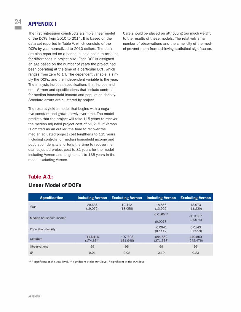
24

APPENDIX I

APPENDIX IThe first regression constructs a simple linear model of the DCFs from 2010 to 2014. It is based on the data set reported in Table V, which consists of the DCFs by year normalized to 2010 dollars. The data are also reported on a per-household basis to account for differences in project size. Each DCF is assigned an age based on the number of years the project had been operating at the time of a particular DCF, which ranges from zero to 14. The dependent variable is sim-ply the DCFs, and the independent variable is the year. The analysis includes specifications that include and omit Vernon and specifications that include controls for median household income and population density. Standard errors are clustered by project.

The results yield a model that begins with a nega-tive constant and grows slowly over time. The model predicts that the project will take 115 years to recover the median adjusted project cost of $2,215. If Vernon is omitted as an outlier, the time to recover the median adjusted project cost lengthens to 125 years. Including controls for median household income and population density shortens the time to recover me-dian adjusted project cost to 81 years for the model including Vernon and lengthens it to 136 years in the model excluding Vernon.

Care should be placed on attributing too much weight to the results of these models. The relatively small number of observations and the simplicity of the mod-el prevent them from achieving statistical significance.

Table A-1:

Linear Model of DCFs

Specification Including Vernon Excluding Vernon Including Vernon Excluding Vernon

Year20.636 (19.072)

19.412 (18.058)

18.856 (13.929)

13.073 (11.230)

Median household income-0.0165**

(0.0077)

-0.0150* (0.0074)

Population density-0.0941 (0.1112)

0.0143 (0.0559)

Constant-144.416 (174.654)

-197.308 (161.948)

684.869 (371.567)

440.859 (242.476)

Observations 99 95 99 95

R2 0.01 0.02 0.10 0.23

*** significant at the 99% level, ** significant at the 95% level, * significant at the 90% level

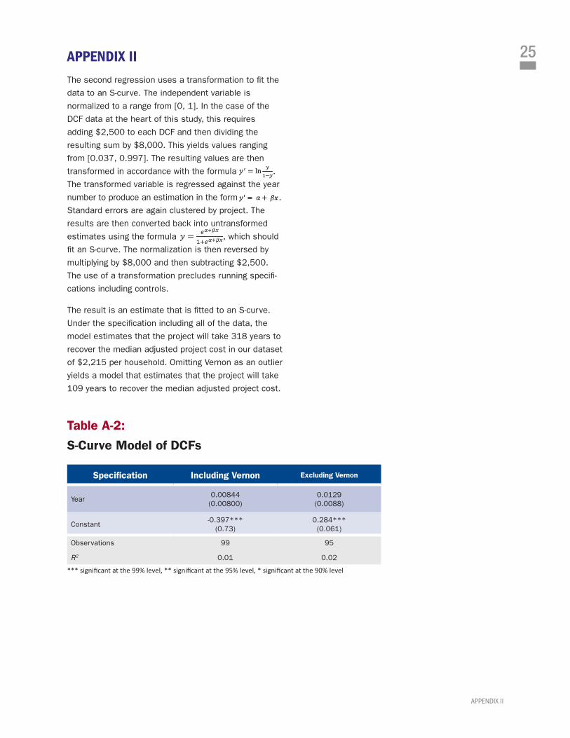
25

APPENDIX II

APPENDIX IIThe second regression uses a transformation to fit the

data to an S-curve. The independent variable is

normalized to a range from [0, 1]. In the case of the

DCF data at the heart of this study, this requires

adding $2,500 to each DCF and then dividing the

resulting sum by $8,000. This yields values ranging

from [0.037, 0.997]. The resulting values are then

transformed in accordance with the formula .

The transformed variable is regressed against the year

number to produce an estimation in the form .

Standard errors are again clustered by project. The

results are then converted back into untransformed

estimates using the formula , which should

fit an S-curve. The normalization is then reversed by

multiplying by $8,000 and then subtracting $2,500.

The use of a transformation precludes running specifi-

cations including controls.

The result is an estimate that is fitted to an S-curve.

Under the specification including all of the data, the

model estimates that the project will take 318 years to

recover the median adjusted project cost in our dataset

of $2,215 per household. Omitting Vernon as an outlier

yields a model that estimates that the project will take

109 years to recover the median adjusted project cost.

Table A-2:

S-Curve Model of DCFs

Specification Including Vernon Excluding Vernon

Year0.00844 (0.00800)

0.0129 (0.0088)

Constant-0.397***

(0.73)0.284*** (0.061)

Observations 99 95

R2 0.01 0.02

*** significant at the 99% level, ** significant at the 95% level, * significant at the 90% level

26

APPENDIX III

APPENDIX IIIThe third regression attempts to measure which factors are driving municipal fiber projects’ successes or failures: revenue generation, operating efficiency, or capital costs. The dependent variable is construct-ed by dividing the adjusted project cost by NPV from 2010 to 2014. This provides a measure of what fraction of the adjusted project cost was recovered during the five-year period running from 2010 to 2014 reported in Table VII.

Regarding the independent variables, the strength of revenue generation is measured by revenue per household in 2014, which as the last year of our study measures the project’s most mature operations. Operating efficiency is measured by operating cost as a percentage of operating revenue in 2014. Capital costs are measured by project cost per household normalized to 2010 dollars.

We ran four specifications. The first includes all 20 of the projects in our data set. The second excludes Vernon as a potential outlier, given that the value for its independent variable is so discontinuous with the other projects, likely driven by the manner in which the project’s commercial nature understates its adjusted project cost per household. We ran specifications that both omit and include population density and median income as controls. The results are as follows:

The results of the regression conducted on the full data set (that is, including Vernon) identify two factors as statistically significant. The regressions that omit Vernon yield statistically significant results for reve-nue per household, which has a t value of 4.15 and a statistical significance of 99.9 percent. The specifica-tion including the controls also yields weak statistical significance for adjusted project cost per household, with a coefficient that is 1.7 times smaller. Although operating efficiency has the largest coefficient and the coefficient has the wrong sign, it lacks the statistical significance to exclude the possibility that it is differ-ent from zero. The R2 for these regressions are 0.87 and 0.90. Overall, such results are remarkable for a data set consisting of only 20 entries.

Excluding Vernon from the data set produces coef-ficients that are similar, but reduces the size of the coefficients for both of the variables found to be statistically significant in the first specification. Most importantly, the specification without the controls identifies operating efficiency as statistically signifi-cant. The magnitude of the coefficient is 25,000 times larger than the coefficient for the other independent variable. Interestingly, including the controls causes the statistical significance to disappear.

Table A-3:

Regression Estimation of Determinants of DCFs

SpecificationIncluding Vernon

Excluding Vernon

Including Vernon

Excluding Vernon

Revenue per household0.000227***

(0.000023)0.0000309 (0.0000408)

0.000168*** (0.000041)

0.0000217 (0.0000460)

Operating cost per operating revenue-0.160 (0.287)

-0.775*** (0.226)

0.422 (0.417)

-0.475 (0.365)

Adjusted project cost per household-0.0000874 (0.0000525)

-0.0000310 (0.0000361)

-0.0000996* (0.0000503)

-0.0000424 (0.0000377)

Population density-0.0000327 (0.0000550)

-0.0000277 (0.0000381)

Median household income-0.0000145 (0.0000084)

-0.00000575 (0.00000624)

Constant0.106 (0.263)

0.702*** (0.211)

0.298 (0.270)

0.743*** (0.217)

Observations 20 19 20 19

R2 0.87 0.59 0.90 0.63

*** significant at the 99% level, ** significant at the 95% level, * significant at the 90% level

27

REFERENCES

REFERENCESBalhoff, M.J., and Rowe, R.C. Municipal broadband: Digging beneath the surface. Charlotte, NC: Balhoff &

Rowe, LLC, 2005. http://broadband.cti.gr/en/download/Municipal-Broadband—Digging%20Beneath%20the%20Surface.pdf.

Bast, J. Municipally owned broadband networks: A critical evaluation. Chicago: The Heartland Institute, 2002. https://www.heartland.org/_template-assets/documents/publications/10687.pdf.

Bast, J. Municipally owned broadband networks: A critical evaluation (revised edition). Chicago: The Heartland Institute, 2004. https://www.heartland.org/_template-assets/documents/publications/15842.pdf.

Baumgartner, J. “Who needs a gig?” Multichannel News, August 4, 2016. http://www.multichannel.com/blog/bauminator/who-needs-gig/406879.

Becerra, H. “Vernon’s investments lose millions: The city has amassed nearly half a billion in debt and signed ‘risky,’ aggressive deals.” Los Angeles Times, August 14, 2011.

Davidson, C.M., and Santorelli, M.J. Understanding the debate over government-owned broadband networks: Context, lessons learned, and a way forward for policy makers. New York: ACLP at New York Law School, 2014. http://www.nyls.edu/advanced-communications-law-and-policy-institute/wp-content/uploads/sites/169/2013/08/ACLP-Government-Owned-Broadband-Networks-EXEC-SUMM-June-20141.pdf.

Dougherty, C. “Two cities with blazing internet speed search for a killer app.” New York Times, September 5, 2014. https://www.nytimes.com/2014/09/06/technology/two-cities-with-blazing-internet-speed-search-for-a-killer-app.html.

Eisenach, J.A. “Does government belong in the telecom business?” Progress on Point, 8(1) (2001): 1-24. http://www.pff.org/issues-pubs/pops/pop8.1govtintelecom.pdf.

Fiber to the Home Council. “Municipal fiber to the home deployments: Next generation broadband as a munici-pal utility.” McLean, VA: FTTH Council Americas, 2009. http://www.ftthcouncil.org/d/do/69.

Fuhr, J.P., Jr. “The hidden problems with government-owned networks.” Indianapolis, IN: Coalition for the New Economy, 2012. http://www.coalitionfortheneweconomy.org/wp-content/uploads/2012/01/1-6-12- Coalition-for-a-New-Economy-White-Paper.pdf.

Janson, M.A., and Yoo, C.S. “The wires go to war: The U.S. experiment with government ownership of the tele-phone system during World War I.” Texas Law Review, 91(5) (2013): 983 –1050.

Kandutch, C. “The case for municipal broadband: The historical context, the law, the technology, and the future imperative.” Broadband Properties, May 2005, 18-25. http://www.broadbandproperties.com/2005issues/may05issues/Carl_Kandutsch_The_Case_for_Muni_Broadband.pdf.

Kenny, R., and Broughton, T. “Domestic demand for bandwidth: An approach to forecasting requirements for }the period 2013–2023.” London: Broadband Stakeholder Group, 2013. http://www.broadbanduk.org/wp-content/uploads/2013/11/BSG-Domestic-demand-for-bandwidth.pdf.

Lenard, T.M. “Government entry into the telecom business: Are the benefits commensurate with the costs?” Progress on Point, 11(3) (2004): 1-31. http://www.pff.org/issues-pubs/pops/pop11.3govtownership.pdf.

Lohr, S. “U.S. city breaks away from pack in Web access.” International Herald Tribune, September 14, 2010.

McClure, D. “Razzle-dazzle: The case against public broadband.” Broadband Properties, May 2005, 26-29. http://www.broadbandproperties.com/2005issues/may05issues/Dave_McClure_The_Case_AGainst_Public_Broadband.pdf.

Mitchell, C. “Burlington telecom profits from fiber.” Broadband Properties, October 2007, 76-81. http://www.broadbandproperties.com/2007issues/october07/Burlington.pdf.

———. “Learning from Burlington Telecom: Some lessons for community networks.” Minneapolis, MN: New Rules Project, 2011. http://www.muninetworks.org/sites/www.muninetworks.org/files/bt-lessons-learned.pdf.

28

REFERENCES

———. “Broadband at the speed of light: How three communities built next-generation networks.” Washington, DC: Institute for Local Self Reliance, 2012. http://ilsr.org/wp-content/uploads/2012/04/ muni-bb-speed-light.pdf.

Mölleryd, B. “Development of high-speed networks and the role of municipal networks.” OECD Science, Technology and Industry Policy Papers No. 26. Paris: OECD Publishing, 2015. http://www.oecd.org/officialdocuments/publicdisplaydocumentpdf/?cote=DSTI/ICCP/CISP(2015)1/FINAL&docLanguage=En.

Montagne, R., and Chaillou, V. “Public funding & FTTH: Assessing the impact of public action.” Communications & Strategies, 80(4) (2010): 153-161.

Scott, B., and Wellings, F. “Telco lies and the truth about municipal broadband networks.” Washington, DC: Free Press, 2005. http://www.freepress.net/sites/default/files/fp-legacy/mb_telco_lies.pdf.

“The need for speed: What superfast connections can do for a city.” The Economist, August 12, 2012. http://www.economist.com/node/21560288.

Virginia Auditor of Public Accounts. “Review of Bristol Virginia Utilities Authority,” 2016. http://www.apa.virginia.gov/reports/BVUA2016-web.pdf.