MPRAMunich Personal RePEc Archive

Keynes’ Absolute Income Hypothesisand Kuznets Paradox

R. Santos Alimi

Adekunle Ajasin University, Akungba-Akoko, Ondo State Nigeria

26 August 2013

Online at https://mpra.ub.uni-muenchen.de/49310/MPRA Paper No. 49310, posted 26 August 2013 14:05 UTC

1

KEYNES' ABSOLUTE INCOME HYPOTHESIS

AND KUZNETS PARADOX

R. Santos Alimi

Department of Economics,

Adekunle Ajasin University

Akunbga Akoko, Ondo State Nigeria.

Email: rasaq.alimi@aaua.edu.ng, santos4rd@gmail.com

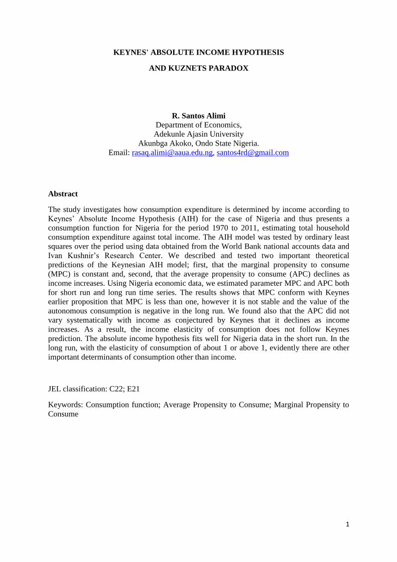
Abstract

The study investigates how consumption expenditure is determined by income according to

Keynes‟ Absolute Income Hypothesis (AIH) for the case of Nigeria and thus presents a

consumption function for Nigeria for the period 1970 to 2011, estimating total household

consumption expenditure against total income. The AIH model was tested by ordinary least

squares over the period using data obtained from the World Bank national accounts data and

Ivan Kushnir‟s Research Center. We described and tested two important theoretical

predictions of the Keynesian AIH model; first, that the marginal propensity to consume

(MPC) is constant and, second, that the average propensity to consume (APC) declines as

income increases. Using Nigeria economic data, we estimated parameter MPC and APC both

for short run and long run time series. The results shows that MPC conform with Keynes

earlier proposition that MPC is less than one, however it is not stable and the value of the

autonomous consumption is negative in the long run. We found also that the APC did not

vary systematically with income as conjectured by Keynes that it declines as income

increases. As a result, the income elasticity of consumption does not follow Keynes

prediction. The absolute income hypothesis fits well for Nigeria data in the short run. In the

long run, with the elasticity of consumption of about 1 or above 1, evidently there are other

important determinants of consumption other than income.

JEL classification: C22; E21

Keywords: Consumption function; Average Propensity to Consume; Marginal Propensity to

Consume

2

1.0 Introduction

Consumption expenditure constitutes the largest proportion of the Gross Domestic Product in

most countries. In the words of Muellbauer and Lattimore (1994:292), „consumer expenditure

accounts for between 50% and 70% of spending in most economies. Not surprisingly, the

consumption function has been most studied of the aggregate expenditure relationships and

has been a key element of all the macroeconomic model building efforts since the seminal

work of Klein and Goldberger (1955).‟ It therefore becomes imperative to investigate how

people spend income in an economy in order to understand consumer behaviour.

Prior to Keynes, consumption had been viewed as a passive residual, the amount of

income remaining after saving. In this view, the decision of any economic agent to save was

determined by the payment for the utility lost from consuming, by implication consumption

was depended on the interest rate - a key factor of saving behaviour (Bunting, 2001). Keynes

observed that "(t)here are not many people who will alter their way of living because the rate

of interest has fallen from 5 to 4 percent" (Keynes, 1936: 94). Thus, the modern consumption

theory begins with his ideal of "fundamental psychological law" of consumption proposed in

his General Theory; “The fundamental psychological law, upon which we are entitled to

depend with great confidence both a priori from our knowledge of human nature and from

the detailed facts of experience, is that men are disposed, as a rule and on the average, to

increase their consumption as their income increases, but not by as much as the increase in

their income”(Keynes, 1936:96).

Keynes postulates that as a rule households increase their utility by consuming more

of the produced goods and services as their income increases. They increase their well-being

by this major component of the aggregate demand. For this reason the possible determinants

of the aggregate consumption function have been analyzed intensively in the economic

literature. Different consumption theories exist in literature; nevertheless, there is no single

theory of consumption that can possibly explain consumption behavior in all economies.

The aim of this study is to investigate how consumption expenditure is determined by

income according to Keynes‟ AIH for the case of Nigeria and test the two important

theoretical predictions of the Keynesian AIH model; first, that the marginal propensity to

consume (MPC) is constant and, second, that the average propensity to consume (APC)

declines as income increases.

2.0 Theoretical Framework and Literature Review

There is need to review the fundamental models of consumptions in order to understand the

modern consumption research. These models are; Keynes‟ (1936) Absolute Income

Hypothesis (AIH), Duesenberry‟s (1949) Relative Income Hypothesis (RIH), Modigliani‟s

(1949) Life Cycle Hypothesis (LCH), Friedman‟s (1957) Permanent Income Hypothesis

(PIH).

Absolute Income Hypothesis

Research on the aggregate consumption function is thought to have begun with Keynes‟s

General Theory, though we need not disregard excellent earlier work of Ramsey (1928) and

Fischer (1930). Since then consumption has been the subject of countless theoretical and

3

empirical studies. Keynes treated consumption on a very “common sense” level. He relied

almost entirely on intuition - like most other economists of his day, his methods included

neither mathematical theory nor detailed econometrics, as he demonstrated the central

principle of his consumption theory. According to Keynes an economic agent by natural

instinct tend as a rule and on the average, to increase his consumption as his income rises, but

not by as much as the increase in his income. In his work on the relationship between income

and consumption, he came out with the finding that income is the sole determinant of

consumption (Tsenkwo, 2011). Keynes gave no basis for his theory in terms of utility

maximization nor indeed gave any consideration of why a consumer would behave in the way

he assumed. In place of rational-choice theory, Keynes relied on his “knowledge of human

nature.” Moreso, he did not give any support to his postulate using numerical data, rather he

claimed to glean support from “detailed facts of experience.” While Keynes placed

consumption theory at the center of the macroeconomic stage, he left it for future generations

of economists to work out the micro-foundations for his theory. Keynes also inspired

pioneers in the emerging field of econometrics to swarm over the newly invented national

income and product statistics looking for verification or refutation of his model (Parker,

2010).

Based on Keynesian consumption function, the Absolute Income Hypothesis (AIH,

hereafter), aggregate consumption is a stable, but not necessarily linear, function of

disposable income,

Ct = α + βYt (1)

where Ct and Yt denote the (real values of) total personal consumption expenditure and total

disposable income, respectively at time t. β, the marginal propensity to consume (MPC) is

expected to be constant and positive but less than unity, so that higher income leads to higher

consumption. The autonomous component of consumption, α, is assumed to be small but

positive. By capturing the conjectures of the fundamental law, the absolute income

hypothesis has these important features: (1) that the consumption expenditure increases or

decreases with increase or decrease in income but non-proportionally. This non-proportional

consumption function implies that in the short run average propensity to consume (APC) is

greater than the MPC: APC > MPC, where APC =

and MPC =

; this is because in the

short run autonomous consumption do not change with income but over the long period

horizon, as wealth and income increase, consumption also rises; the marginal propensity to

consume out of the long run income is closer to the average propensity to consume. (2) as

income rises, the proportion of it consumed falls:

< 0, so the income elasticity of

consumption defined as

would be less than unity. (3) that consumption function is stable

both in the short run and long run.

The Kuznets Paradox

The early econometric history of the consumption function made efforts to test the

relationship between consumption and income as proposed by the absolute income

hypothesis with available data, using whatever specification seemed reasonable (Bunting,

2001). Almost all empirical studies that were either cross-sectional or short-run time-series

supported Keynes‟s postulation on consumption. However, the seminal study made by

Kuznets (1946) - a Nobel prize winner was a turning point in the development of the

consumption function literature, because his study made use of long-run time series (see

Thomas, 1989). Kuznets showed that except for the Depression years, the APC in the U.S.

4

over the period 1869–1938 fluctuated narrowly between 0.84 and 0.89. In other words, APC

was approximately mean-reverted, such that even if income increased a lot, consumption kept

almost a stable fraction of income; so consumption was a proportion rather than a function of

income (Baykara and Telatar, n.d). These empirical inconsistent is referred to as Kuznets

puzzle or consumption puzzle as Friedman (1957) termed it, a seemingly contradictory fact

with the assumptions made by the AIH.

Relative Income Hypothesis (RIH)

One of the earliest attempts to reconcile these conflicting pieces of evidence about the

consumption-income relationship was the relative-income hypothesis, described by James

Duesenberry (1949). Although this theory has vanished with hardly a trace from

contemporary macroeconomics, it carried considerable influence in the 1950s and 1960s

(Parker, 2010). Relative income hypothesis states that the satisfaction an individual derives

from a given consumption level depends on its relative magnitude in the society (e.g., relative

to the average consumption) rather than its absolute level. It is based on a postulate that has

long been acknowledged by psychologists and sociologists, namely that individuals care

about status (Kockesen, n.d.). In economics, relative income hypothesis is attributed to James

Duesenberry (1949), who investigated the implications of this idea for consumption behavior

in his book titled Income, Saving and the Theory of Consumer Behavior. Duesenberry

proposes an individual consumption function that depends on the current income of other

people and as a result, „„for any given relative income distribution, the percentage of income

saved by a family will tend to be unique, invariant, and increasing function of its percentile

position in the income distribution. The percentage saved will be independent of the absolute

level of income. It follows that the aggregate saving ratio will be independent of the absolute

level of income‟‟ (as cited in Alvarez-Cuadrado & Long, 2011, p. 1489).

Duesenberry argued that relative income hypothesis could account for both the cross-

sectional and time series evidence. He claimed that an individual‟s utility index depended on

the ratio of his or her consumption to a weighted average of the consumption of the others.

From this he drew two conclusions: (1) aggregate saving rate is independent of aggregate

income, which is consistent with the time series evidence; and (2) the propensity to save of an

individual is an increasing function of his or her percentile position in the income

distribution, which is consistent with the cross-sectional evidence. Despite its intuitive and

empirical success, the relative income hypothesis was quickly replaced by the life-

cycle/permanent-income hypothesis of Franco Modigliani and Richard Brumberg (1954) and

Milton Friedman (1957), as the economists‟ workhorse to understand consumption behavior.

These closely related theories implied that consumption is an increasing function of the

expected lifetime resources of an individual and could account for both the cross-sectional

and time series.

Life Cycle Hypothesis (LCH)

Modigliani and Brumberg‟s (1954 and 1980) life cycle hypothesis was designed to reconcile

the discrepancy between cross-sectional findings and the findings of time-series analysis. In

addition, the model was meant to capture the effect of liquid assets on consumption. Unlike

the Keynesian consumption theory that is entirely based on the current income of the

individuals, the concept of LCH assumes that all individuals consume a constant percentage

5

of present value of their life income. The life-cycle theory assumes that individuals or

families try to maximise the utility deriving from their entire life-cycle consumption.

Therefore consumption must be continuous, even if income through the life-cycle is

discontinuous; and saving is primarily done to finance consumption during the retirement

period (see Kankaanranta, 2006 ). According to Modigliani (1986 and 2001) the „basic‟

version of the life-cycle hypothesis is based on the following assumptions: (1) Income is

constant until retirement, zero thereafter (2) Zero interest rate (3) Preferences: constant

consumption over the life cycle (4) Absence of bequests (Baranzini, 2005).

According to the life cycle hypothesis the average propensity to consume is larger in

the old households and among young people. This is because the old people run their lives on

their life savings while the young people are more into borrowing. The middle-aged people,

on the other hand, incline to have higher incomes with lower consumption and higher saving.

The Life Cycle Hypothesis can be explained by the equation

C = (W + RY) / T (2)

Where W = Initial endowed wealth, R = Number of years earning labor income, Y = Labour

Income, and T = Number of years of the individual's lifespan.

Rewriting the equation or consumption function in equation (2)

C =

W +

Y (3)

If every individual plans their consumption in such way, the aggregate consumption function

of the economy, will take the form

C = W + δY (4)

where parameter (=

) is the marginal propensity to consume out of accumulated wealth and

δ (=

) is the marginal propensity to consume out of income.

The first result of this model is that the marginal propensity to consume (MPC)

depends on whether a change in income is expected to be temporary or permanent. First,

consider a temporary change in current income, which can be considered equivalent to a

change in current wealth, WR. Taking the derivative of average annual consumption,

equation (4), with respect to initial wealth, W, and we get the marginal propensity to consume

out of a temporary change in income. The marginal propensity to consume out of a temporary

change in income will always be equal to 1 divided by the number of years an economic

agent expects to live. Whereas, the marginal propensity to consume out of a change in labour

income is always the number of years of labor divided by the number of years the household

expects to live.

Permanent Income Hypothesis (PIH)

In response to this empirical puzzle, Milton Friedman (1957) proposed his permanent income

hypothesis (PIH) which maintains that households spend a fixed fraction of their permanent

income on consumption. Unlike AIH, the PIH was inspired by micro-foundations and

representative agents, and highlighted the importance of not just the present but also future.

6

The core of Friedman‟s PIH was that individuals want to maximize their lifetime well-being

(utility) subject to the constraint that all their lifetime resources must be spent. The

Friedman‟s theory focused on distinguishing between consumption and current expenditure

on the one hand, and income and current receipts on the other hand. This is because an

individual economic agent is thought to plan his expenditures on both income received during

the current period and income expected during his lifetime. Therefore, consumers plan their

expenditure on the grounds of a long-run view of the resources that will accrue to them in

their lifetime.

As a result, Friedman postulated that income, Y, is made up of two components: a

permanent component (YP) and transitory component (Y

T). Friedman argued that some of the

factors that give rise to the transitory component of income were specific to particular

consumer but that for any considerable group of consumers the transitory components tend to

average out so that the mean of the transitory component is expected to be zero. On the

corollary, consumption expenditures comprise permanent (CP) and transitory components

(CT). The permanent component relates to the amount that consumers plan to consume to

maximize their lifetime utility. Without uncertainty, total consumption would be equal to CP.

CT relates to all „other‟ factors. (Fernandez-Corugedo, 2004)

The PIH gives rise to a consumption function of the form:

CP = k(r, w, u) x Y

p (5)

Y = YP + Y

T (6)

C = CP + C

T (7)

where C = current consumption spending, CP = permanent consumption, C

T = transitory

consumption, Y = current income, YP = permanent income, Y

T = transitory income, r = rate

of interest at which the consumer can borrow or lend, w = ratio of wealth to income and u =

consumer‟s taste preferences. Equation (5) defines the relationship between permanent

consumption and permanent income, and the marginal propensity to consume out of

permanent income, k(·) is independent of the size of permanent income but it does depend on

other variables: r, w and u. The equations (6) and (7) provide a means of linking actual

measured variables (C, Y) to their relevant components (Fernandez-Corugedo, 2004).

Under permanent income theory, the MPC is constant and equal to the APC, which is

consistent with Kuznets‟ (1946) empirical findings. The MPC is also the same for all

households. Friedman reconciled the difference between cross-section regression estimates of

consumption and long run aggregate time series regression estimates by appeal to a statistical

“errors-in-variables” argument. The argument is that cross section estimates use actual

household income rather than permanent household income. Owing to the fact that more

households are situated in the middle of the income distribution, the observed distribution of

actual household income tends to be more spread out than permanent income. Consequently,

regression estimates using actual income tend to find a flatter slope, and hence the finding

that cross section consumption function estimates are flatter than time series aggregate per

capita consumption function estimates. Friedman‟s PIH therefore offered a simple

explanation of the empirical consumption puzzle. At the theoretical level, the innovation was

the construct of permanent income that introduced income expectations, thereby adding a

sensible forward-looking dimension to consumption theory (Palley, 2008). The Friedman‟s

theory had important implications for fiscal policy. First, since all households have the same

MPC it undermined the Keynesian demand stimulus argument for progressive taxation.

7

Second, it introduces a distinction between permanent and temporary tax shocks. For policy

makers, the source and nature of the shocks are important. For instance, an announcement

that tax cuts will be permanent would lead to different behavior of household/firm economic

agent compared to when such tax changes are thought to only be transitory.

3.0 DATA AND METHODS

We use gross national income as a proxy for income and household final consumption

expenditure as a proxy for consumption. Data for the series arein US billion dollar and are

collected from World Bank national accounts data, OECD National Accounts data files and

Ivan Kushnir‟s Research Center. The data is annual and spans the time period from 1970-

2011, total are 41 years. We start by defining YGNI as the gross national income and CHTCE as

household total consumption expenditure.

We re-specify the Keynesian AIH to be tested empirically using the ordinary least

squares as;

CHTCE = α + βYGNI (8)

Where;

CHTCE = Total Household Consumption Expenditure

α = Autonomous Consumption (independent of the level of income)

β =Marginal Propensity to Consume (MPC), 0 < β < 1

YGNI = Total Disposable Income in year t

In the analysis of the common components of household consumption expenditure and GNI

per capita, standard time series unit root tests can be applied. To ensure robustness we use

several unit root tests, including the Augmented Dickey and Fuller (1979) (ADF) test, the

Phillips and Perron(1988) (PP) test, as well as the Kwiatkowski, Phillips, Schmidt, and Shin

(1992) (KPPS) test. The latter tests the null of stationarity whereas the former two investigate

the null of a unit root. We do not further discuss the details of these well-known time series

unit root tests but instead call attention to Maddala and Kim (1998) for their excellent

treatment of ADF, PP and KPSS. Nelson and Plosser (1982) indicate that many

macroeconomic time series data have a stochastic trend plus a stationary component, that is,

they are difference stationary processes. It is also of great importance to discern the

temporary and permanent movements in an economic time series. Economic theory in this

line assumes that at least some subsets of economic variables do not drift through time

independently of each other and some combination of the variables in these subsets reverts to

the mean of a stable stochastic process. Granger (1986) and Engle and Granger (1987)

indicate that even though economic time series may be non-stationary in their level forms,

there may exist some linear combination of these variables that converge to a long run

relationship over time, which also requires the existence of Granger causality in at least one

direction in an economic sense as one variable can help forecast the others.

A lot of techniques are available to test for the existence of long-run equilibrium

relationships in the levels among variables. Two popular cointegration tests, namely, the

Engle-Granger (EG) test and the Johansen test are used. The EG test is contained in Engle

8

and Granger (1987) while the Johansen test is found in Johansen (1988) and Johansen and

Juselius (1990). The EG test involves testing for stationarity of the residuals. If the residual

series is stationary, the variables CHTCE and YGNI are cointegrated and if it is non-stationary,

the variables are not cointegrated. The EG approach could exhibit some degree of bias arising

from the stationarity test of the residuals from the chosen equation. The EG test assumes one

cointegrating vector in systems with more than two variables and it assumes arbitrary

normalization of the cointegrating vector. Nevertheless we adopted EG test because the

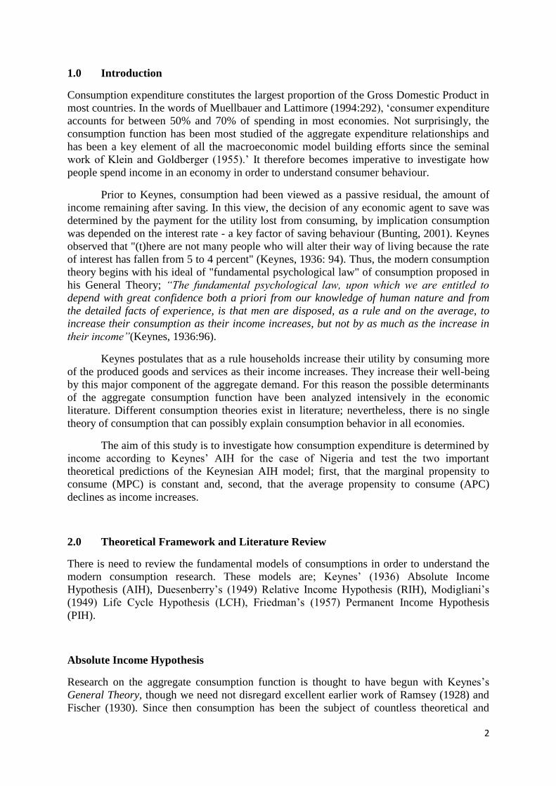
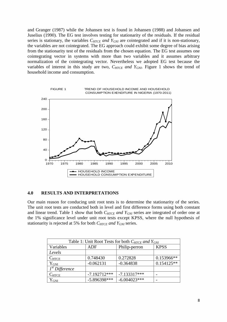
variables of interest in this study are two, CHTCE and YGNI. Figure 1 shows the trend of

household income and consumption.

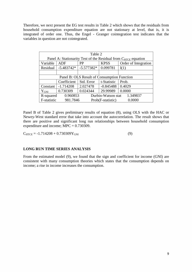
4.0 RESULTS AND INTERPRETATIONS

Our main reason for conducing unit root tests is to determine the stationarity of the series.

The unit root tests are conducted both in level and first difference forms using both constant

and linear trend. Table 1 show that both CHTCE and YGNI series are integrated of order one at

the 1% significance level under unit root tests except KPSS, where the null hypothesis of

stationarity is rejected at 5% for both CHTCE and YGNI series.

Table 1: Unit Root Tests for both CHTCE and YGNI

Variables ADF Philip-perron KPSS

Levels

CHTCE 0.748430 0.272828 0.153966**

YGNI -0.062131 -0.364838 0.154125**

1st Difference

CHTCE -7.192712*** -7.133317*** -

YGNI -5.896398*** -6.004023*** -

0

40

80

120

160

200

240

1970 1975 1980 1985 1990 1995 2000 2005 2010

HOUSEHOLD INCOMEHOUSEHOLD CONSUMPTION EXPENDITURE

FIGURE 1 TREND OF HOUSEHOLD INCOME AND HOUSEHOLD

CONSUMPTION EXENDITURE IN NIGERIA (1970-2011)

9

Therefore, we next present the EG test results in Table 2 which shows that the residuals from

household consumption expenditure equation are not stationary at level, that is, it is

integrated of order one. Thus, the Engel - Granger cointegration test indicates that the

variables in question are not cointegrated.

Table 2

Panel A: Stationarity Test of the Residual from CHTCE equation

Variable ADF PP KPSS Order of Integration

Residual -5.483742* -5.577382* 0.099781 I(1)

Panel B: OLS Result of Consumption Function

Coefficient Std. Error t-Statistic Prob.

Constant -1.714208 2.027478 -0.845488 0.4029

YGNI 0.730309 0.024344 29.99989 0.0000

R-squared 0.960853 Durbin-Watson stat 1.349837

F-statistic 981.7846 Prob(F-statistic) 0.0000

Panel B of Table 2 gives preliminary results of equation (8), using OLS with the HAC or

Newey-West standard error that take into account the autocorrelation. The result shows that

there are positive and significant long run relationships between household consumption

expenditure and income; MPC = 0.730309.

CHTCE = -1.714208 + 0.730309YGNI (9)

LONG RUN TIME SERIES ANALYSIS

From the estimated model (9), we found that the sign and coefficient for income (GNI) are

consistent with many consumption theories which states that the consumption depends on

income; a rise in income increases the consumption.

10

0

20

40

60

80

100

120

140

160

0 20 40 60 80 100 120 140 160 180 200 220 240

HOUSEHOLD INCOME

HO

US

EH

OL

D O

NS

UM

PT

ION

EX

PE

ND

ITU

RE

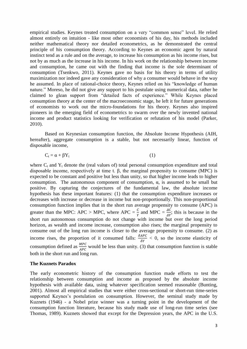
FIGURE 2: HOUSEHOLD CONSUMPTION EXPENDITURE

VERSUS HOUSEHOLD INCOME (1970-2011)

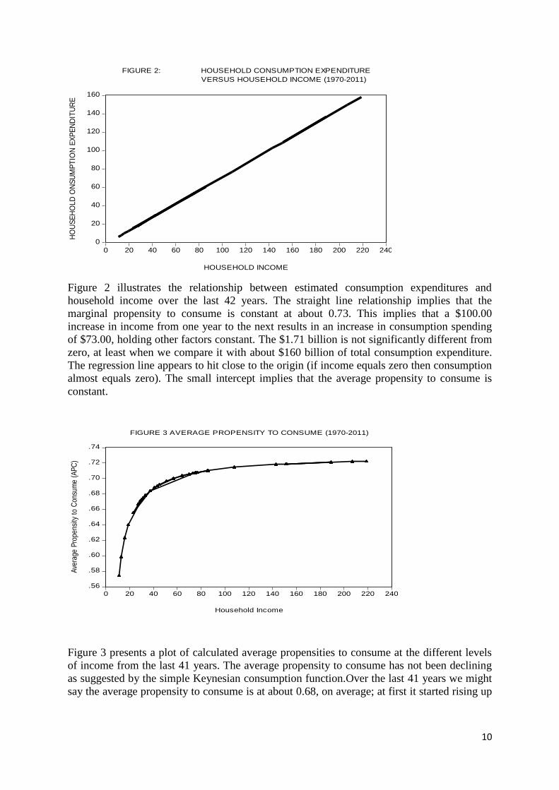
Figure 2 illustrates the relationship between estimated consumption expenditures and

household income over the last 42 years. The straight line relationship implies that the

marginal propensity to consume is constant at about 0.73. This implies that a $100.00

increase in income from one year to the next results in an increase in consumption spending

of $73.00, holding other factors constant. The $1.71 billion is not significantly different from

zero, at least when we compare it with about $160 billion of total consumption expenditure.

The regression line appears to hit close to the origin (if income equals zero then consumption

almost equals zero). The small intercept implies that the average propensity to consume is

constant.

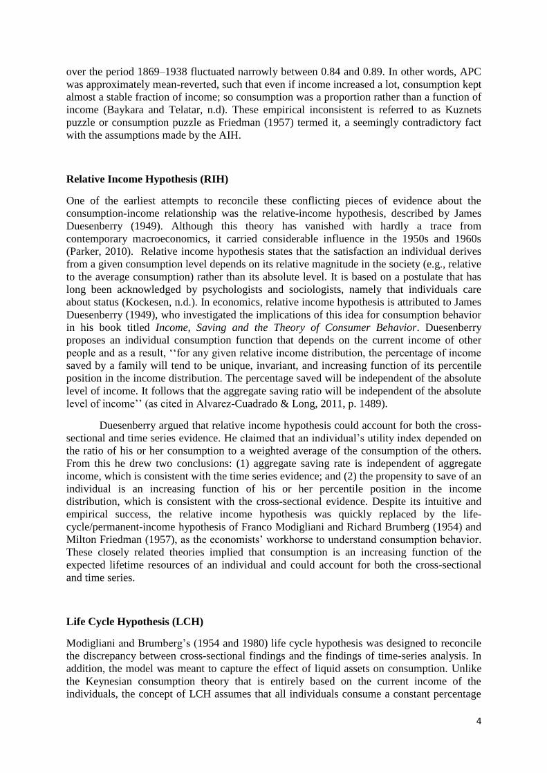
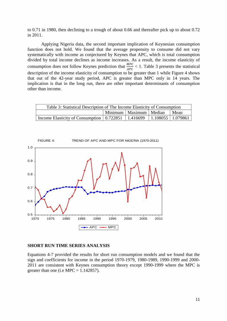
Figure 3 presents a plot of calculated average propensities to consume at the different levels

of income from the last 41 years. The average propensity to consume has not been declining

as suggested by the simple Keynesian consumption function.Over the last 41 years we might

say the average propensity to consume is at about 0.68, on average; at first it started rising up

.56

.58

.60

.62

.64

.66

.68

.70

.72

.74

0 20 40 60 80 100 120 140 160 180 200 220 240

Household Income

Ave

rage

Pro

pens

ity t

o C

onsu

me

(AP

C)

FIGURE 3 AVERAGE PROPENSITY TO CONSUME (1970-2011)

11

to 0.71 in 1980, then declining to a trough of about 0.66 and thereafter pick up to about 0.72

in 2011.

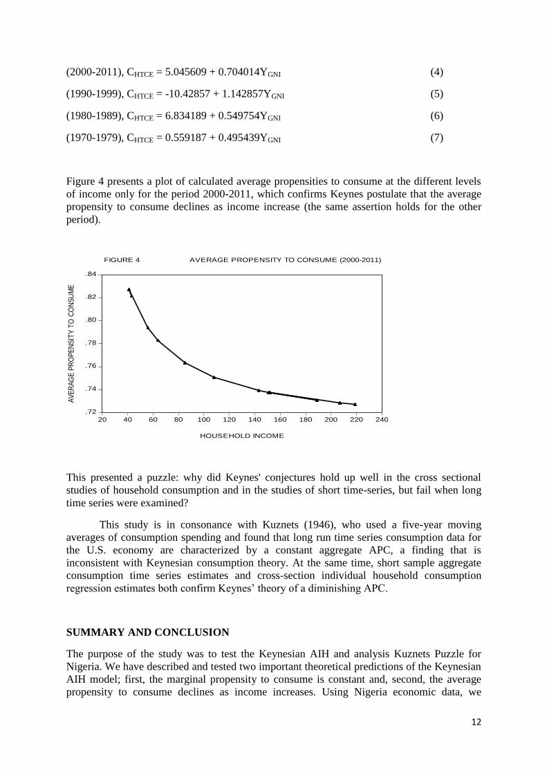
Applying Nigeria data, the second important implication of Keynesian consumption

function does not hold. We found that the average propensity to consume did not vary

systematically with income as conjectured by Keynes that APC, which is total consumption

divided by total income declines as income increases. As a result, the income elasticity of

consumption does not follow Keynes prediction that

< 1. Table 3 presents the statistical

description of the income elasticity of consumption to be greater than 1 while Figure 4 shows

that out of the 42-year study period, APC is greater than MPC only in 14 years. The

implication is that in the long run, there are other important determinants of consumption

other than income.

Table 3: Statistical Description of The Income Elasticity of Consumption

Minimum Maximum Median Mean

Income Elasticity of Consumption 0.722851 1.416699 1.108055 1.079861

SHORT RUN TIME SERIES ANALYSIS

Equations 4-7 provided the results for short run consumption models and we found that the

sign and coefficients for income in the period 1970-1979, 1980-1989, 1990-1999 and 2000-

2011 are consistent with Keynes consumption theory except 1990-1999 where the MPC is

greater than one (i.e MPC = 1.142857).

0.5

0.6

0.7

0.8

0.9

1.0

1970 1975 1980 1985 1990 1995 2000 2005 2010

APC MPC

FIGURE 4: TREND OF APC AND MPC FOR NIGERIA (1970-2011)

12

(2000-2011), CHTCE = 5.045609 + 0.704014YGNI (4)

(1990-1999), CHTCE = -10.42857 + 1.142857YGNI (5)

(1980-1989), CHTCE = 6.834189 + 0.549754YGNI (6)

(1970-1979), CHTCE = 0.559187 + 0.495439YGNI (7)

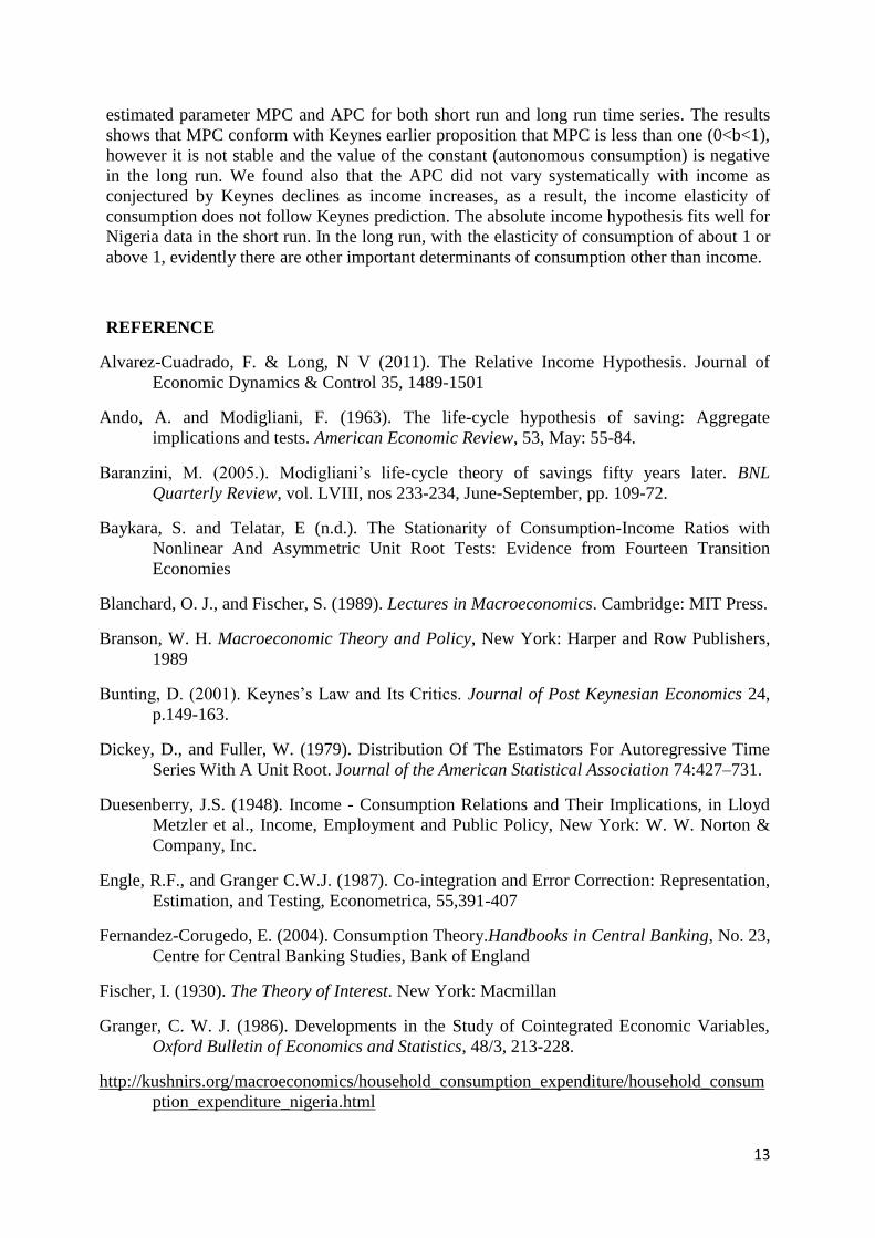
Figure 4 presents a plot of calculated average propensities to consume at the different levels

of income only for the period 2000-2011, which confirms Keynes postulate that the average

propensity to consume declines as income increase (the same assertion holds for the other

period).

This presented a puzzle: why did Keynes' conjectures hold up well in the cross sectional

studies of household consumption and in the studies of short time-series, but fail when long

time series were examined?

This study is in consonance with Kuznets (1946), who used a five-year moving

averages of consumption spending and found that long run time series consumption data for

the U.S. economy are characterized by a constant aggregate APC, a finding that is

inconsistent with Keynesian consumption theory. At the same time, short sample aggregate

consumption time series estimates and cross-section individual household consumption

regression estimates both confirm Keynes‟ theory of a diminishing APC.

SUMMARY AND CONCLUSION

The purpose of the study was to test the Keynesian AIH and analysis Kuznets Puzzle for

Nigeria. We have described and tested two important theoretical predictions of the Keynesian

AIH model; first, the marginal propensity to consume is constant and, second, the average

propensity to consume declines as income increases. Using Nigeria economic data, we

.72

.74

.76

.78

.80

.82

.84

20 40 60 80 100 120 140 160 180 200 220 240

HOUSEHOLD INCOME

AV

ER

AG

E P

RO

PE

NS

ITY

TO

CO

NS

UM

E

FIGURE 4 AVERAGE PROPENSITY TO CONSUME (2000-2011)

13

estimated parameter MPC and APC for both short run and long run time series. The results

shows that MPC conform with Keynes earlier proposition that MPC is less than one (0<b<1),

however it is not stable and the value of the constant (autonomous consumption) is negative

in the long run. We found also that the APC did not vary systematically with income as

conjectured by Keynes declines as income increases, as a result, the income elasticity of

consumption does not follow Keynes prediction. The absolute income hypothesis fits well for

Nigeria data in the short run. In the long run, with the elasticity of consumption of about 1 or

above 1, evidently there are other important determinants of consumption other than income.

REFERENCE

Alvarez-Cuadrado, F. & Long, N V (2011). The Relative Income Hypothesis. Journal of

Economic Dynamics & Control 35, 1489-1501

Ando, A. and Modigliani, F. (1963). The life-cycle hypothesis of saving: Aggregate

implications and tests. American Economic Review, 53, May: 55-84.

Baranzini, M. (2005.). Modigliani‟s life-cycle theory of savings fifty years later. BNL

Quarterly Review, vol. LVIII, nos 233-234, June-September, pp. 109-72.

Baykara, S. and Telatar, E (n.d.). The Stationarity of Consumption-Income Ratios with

Nonlinear And Asymmetric Unit Root Tests: Evidence from Fourteen Transition

Economies

Blanchard, O. J., and Fischer, S. (1989). Lectures in Macroeconomics. Cambridge: MIT Press.

Branson, W. H. Macroeconomic Theory and Policy, New York: Harper and Row Publishers,

1989

Bunting, D. (2001). Keynes‟s Law and Its Critics. Journal of Post Keynesian Economics 24,

p.149-163.

Dickey, D., and Fuller, W. (1979). Distribution Of The Estimators For Autoregressive Time

Series With A Unit Root. Journal of the American Statistical Association 74:427–731.

Duesenberry, J.S. (1948). Income - Consumption Relations and Their Implications, in Lloyd

Metzler et al., Income, Employment and Public Policy, New York: W. W. Norton &

Company, Inc.

Engle, R.F., and Granger C.W.J. (1987). Co-integration and Error Correction: Representation,

Estimation, and Testing, Econometrica, 55,391-407

Fernandez-Corugedo, E. (2004). Consumption Theory.Handbooks in Central Banking, No. 23,

Centre for Central Banking Studies, Bank of England

Fischer, I. (1930). The Theory of Interest. New York: Macmillan

Granger, C. W. J. (1986). Developments in the Study of Cointegrated Economic Variables,

Oxford Bulletin of Economics and Statistics, 48/3, 213-228.

http://kushnirs.org/macroeconomics/household_consumption_expenditure/household_consum

ption_expenditure_nigeria.html

14

Jeffrey Parker. (2010). 16 Theories of Consumption and Saving (Economics 314 Coursebook).

Retrieved from www.academic.reed.edu/economics/parker/

Johansen, S. & Juselius, K., (1990). Maximum likelihood estimation and inference on

cointegration – with applications to the demand for money. Oxford Bulletin of

Economics and Statistics. 52, 2:169-210.

Johansen, S. (1988). Statistical Analysis of Cointegration Vectors, Journal of Economic

Dynamic, 12(1): 231-254.

Kankaanranta, P. (2006). Consumption Over the Life Cycle: A Selected Literature Review.

Aboa Centre for Economics, Discussion Paper No. 7.

Keynes, John Maynard. 1936. The General Theory of Employment, Interest and Money. New

York: Harcourt, Brace.

Kockesen, L. (n.d.). Relative Income Hypothesis. International Encyclopedia of the Social

Science, 2nd Edition p. 153

Kuznets, S. (1946). National Product Since 1869 (assisted by L. Epstein and E. Zenks), New

York: National Bureau of Economic Research.

Kwiatkowski, D. et al. (1992). Testing the Null Hypothesis of Stationarity against the

Alternative of a Unit Root. Journal of Economics, 54, 159-178.

Maddala, G. S. and Kim, I. (1998). Unit roots, cointegration, and structural change.

Cambridge: Cambridge University Press.

Modigliani, F. (1986). Life Cycle, Individual Thrift, and the Wealth Of Nations. Nobel

Lecture delivered in Stockholm, Sweden, December 9, 1985, The AmericanEconomic

Review, vol. 76, no. 3, pp. 297-313.

Modigliani, F. (2001). Adventures of an Economist. Texere, New York and London.

Modigliani, F. and Ando, A. (1957). Tests of the Life Cycle Hypothesis of Saving: Comments

and Suggestions. Bulletin of the Oxford University Institute of Statistics, Vol. 19, pp.

99-124.

Modigliani, F. and Brumberg, R. (1954). Utility Analysis and the Consumption Function: An

Interpretation of Cross-Section Data in K.K. Kurihara ed., PostKeynesian Economics,

(pp. 388-436), Rutgers University Press, New Brunswick.

Modigliani, F. and Brumberg, R. (1980).Utility Analysis and Aggregate Consumption

Functions: An Attempt at Integration in A. Abel ed., The Collected Papers ofFranco

Modigliani, MIT Press, Cambridge, Mass.

Muellbauer, J. N. and Lattimore, R. (1994). The Consumption Function: A Theoretical and

Empirical Overview in Pesaran, H. and Wickens, M.R. (eds) Handbook of Applied

Econometrics.

Nelson, C., and C. Plosser (1982). Trends And Random Walks In Macroeconomics Time

Series: Some Evidence And Implications. Journal of Monetary Economics 10: 139-

162.

15

Palley, T. I. (2008). Relative Permanent Income and Consumption: A Synthesis of Keynes,

Duesenberry, Friedman, and Modigliani and Brumbergh. Political Economy Research

Institute, UMASS, Working Paper Series, Number 170

Phillips, P.C.B., and P. Perron (1988). Testing For Unit Roots In Time Series. Biometrika 75:

335–346.

Ramsey, F. P. (1928). A mathematical Theory of Saving. Economic Journal, 38, pp 543-559

Thomas, J. (1989). The Early History of The Consumption Function. Oxford Economic Papers

41, p131-149.

Tsenkwo, J.B. (2011). Testing Nigeria's Marginal Propensity to Consume (MPC) Within the

Period 1980-2004. Journal of Innovative Research in Management and Humanities,

2(1), April.