Munich Personal RePEc Archive - uni-muenchen.de · Traditional static portfolio selection models, such as Markowitz™s (1952), assume that the distribution of asset returns is objectively

MPRAMunich Personal RePEc Archive

A Simple Model of Robust PortfolioSelection

Marco Taboga

1. June 2004

Online at http://mpra.ub.uni-muenchen.de/16472/MPRA Paper No. 16472, posted 29. July 2009 20:13 UTC

http://mpra.ub.uni-muenchen.de/

http://mpra.ub.uni-muenchen.de/16472/

A Simple Model of Robust Portfolio Selection

Marco Taboga�

([email protected])Università di Torino

January 2004 (last revision June 2004)

Abstract

We propose a single-period portfolio selection model which allowsthe decision maker to easily deal with uncertainty about the distrib-ution of asset returns. The model is preference-based and relies upona separate parametrization of risk aversion and ambiguity aversion.A particular speci�cation of preferences allows us to solve the portfo-lio selection problem and obtain a simple closed-form expression forthe portfolio weights, which lends itself to a straightforward economicinterpretation.

�I thank E. Castagnoli, P. Klibano¤, E. Luciano, F. Maccheroni, M. Marinacci, S.Mukerji for helpful comments and suggestions.

1

Traditional static portfolio selection models, such as Markowitz�s (1952),

assume that the distribution of asset returns is objectively known to the de-

cision maker. Of course, this is hardly a realistic assumption, since at best

investors can estimate the distribution of asset returns with limited preci-

sion. Typically, one assumes that the distribution of asset returns belongs

to a given parametric family and then estimates the relevant parameters us-

ing historical data, hence being left with some uncertainty about the true

parameters. Although the lack of realism of an assumption is not su¢ cient

to disqualify a model, many researchers have argued that uncertainty about

the distribution of asset returns cannot be neglected, since the optimal port-

folios derived within traditional models seem to be highly sensitive to small

changes in the parameters characterizing the distribution.

We adopt a Bayesian framework to model parameter uncertainty, basing

the portfolio selection process on a speci�cation of preferences which allows

a simple and separate parametrization of the investor�s attitudes towards

parameter uncertainty and investment risk.

We assume that the investor maximizes the following objective function,

recently axiomatized by Klibano¤, Marinacci and Mukerji (2003):

E�h'�E�hu�fW�i�i

where fW is stochastic future wealth, ' and u are increasing and concave

functions and � and � are probability measures. The inner expectation (w.r.t.

the measure �) is akin to a von-Neumann Morgenstern expected utility. The

investor realizes that to di¤erent distributions of asset returns correspond

di¤erent values of the expected utility of wealth. The measure � assigns

second-order probabilities to the distributions which are deemed plausible by

the investor and hence to the di¤erent values taken by the expected utility.

Instead of simply averaging over expected utilities, the decision maker applies

a concave transform before taking the outer expectation, hence displaying

aversion to those situations in which parameter uncertainty leads to a great

2

dispersion of expected utility values.

Since the Seventies a wealth of studies documenting and discussing the

importance of parameter uncertainty in portfolio selection models began to

appear: among them Frankfurter, Phillips and Seagle (1971), Barry (1974),

Bawa and Klein (1976) and Jobson and Korkie (1980). Also, a widespread

opinion came about that portfolios constructed using sample moments of

returns often involve very extreme positions, which are far from being truly

optimal: Green and Holli�eld (1992) provide a rigorous analysis of this claim.

As a follow up to these critiques some proposals were made to improve

upon Markowitz�s (1952) model: for example, Frost and Savarino (1988)

and Black and Litterman (1992) propose Bayesian procedures to improve

the performance of estimated optimal portfolios. A very recent work by

Jagannathan and Ma (2003) also gives a contribution to the debate: they

discuss how imposing constraints on portfolio weights can sometimes improve

the performance of estimated optimal portfolios.

The aforementioned studies are aimed at devising methods of correcting

Markowitz�s (1952) optimal allocation rule, in order to improve its perfor-

mance in the presence of parameter uncertainty. Our paper is aimed at a

di¤erent direction: adopting a Bayesian perspective, we propose a model in

which parameter uncertainty is easily and directly quanti�able and becomes

a further variable of the decision problem, besides risk and return.

Our paper belongs to a strand of the literature which tackles the problem

of parameter uncertainty in portfolio selection by specifying the decision-

maker preferences both towards investment risk and towards parameter un-

certainty and by �nding allocation rules consistent with these preferences.

The main idea underlying most studies is that portfolio selection problems

lend themselves to be analyzed with decision-theoretic tools which deviate

from the orthodoxy of the subjective expected utility framework. In these

models a behavioral distinction is made between risk and uncertainty. The

distinction goes back to Knight (1921), who identi�ed two kinds of uncer-

3

tainty: the �rst one is risk, arising in situations where the decision maker is

able to unambiguously assign probabilities to the events which are relevant

to her decision; the second one is ambiguity or Knightian uncertainty, aris-

ing when the probabilities of some events are not unanimously and uniquely

agreed upon. A portfolio selection problem whose parameters are not objec-

tively known would seem to fall into the latter of these two categories. Such

a view is undoubtedly prone to many criticisms, since the standard model of

decision-making, whose foundations were laid out by Savage (1954), does not

allow for a meaningful distinction between risk and ambiguity: according to

that model, the fact that an objectively given distribution of asset returns

is not available to the investor does not prevent her from forming a unique

subjective probability distribution, upon which she can base her decisions.

A consequence of Savage�s postulates is that information is never too im-

precise to be summarized by probabilities. However, many theorists have

argued that in some situations Savage�s model does not allow to distinguish

di¤erences in the quality and the abundance of information used to form

subjective probability distributions: Ellsberg�s (1961) paradox is one of the

pieces of evidence usually cited in support of this view.

Several modelling devices have been used to incorporate ambiguity into

�nancial decision problems. A taxonomy has been proposed by Uppal and

Wang (2003), who identify two main classes of models.

A �rst class of models is inspired by Gilboa and Schmeidler�s (1989) model

of multiple priors preferences. Among them, Epstein andWang (1994) extend

the Lucas (1978) general equilibrium model with multiple priors preferences

and derive asset pricing and equilibrium implications; Dow and Werlang

(1992) set up a static portfolio choice problem with a single risky (and am-

biguous) asset and a single agent with Schmeidler and Gilboa�s preferences;

Chen and Epstein (2002) develop a continuous-time model and the consid-

erable simpli�cations a¤orded by continuous-time modelling allow them to

derive closed formulas for the optimal portfolio allocation.

4

A second class of models makes use of some tools borrowed from the ro-

bust control literature: Maenhout (2004) adapts a framework developed by

Anderson, Hansen and Sargent (2003) to derive a portfolio selection model

set in continuous time, where the decision maker has got a preference for

robustness; Maenhout�s (2004) model, which extends the classical Merton�s

(1990) model, assumes that the decision maker has got a reference probabil-

ity measure over asset returns, but she considers also alternative probability

measures, equivalent to the reference measure (in the probabilistic sense of

equivalence), and she chooses among these measures according to a penalty

function based on the relative entropy between the probability measures.

Uppal and Wang (2003) extend Maenhout�s model to take into account mul-

tiple sources of uncertainty and shed some light on real world phenomena

such as underdiversi�cation and the home bias. Both Maenhout and Uppal

and Wang provide closed formulas for the optimal portfolios.

Among the models we have cited, none provides an asset allocation rule

for the simplest case of a one-period horizon and a single investor. There

are, however, some studies in this direction: Krasker (1982), for example,

analyzes the implications of minimax behavior for portfolio choice; in his

model the agent minimizes over a set of probability measures obtained by

"-contamination of a reference measure; Krasker shows how some commonly

held portfolios (portfolios without short positions or portfolios replicating the

market portfolio) can be rationalized by individual minimax behavior, rather

than on equilibrium considerations. Also Becker, Marty and Rustem (2000)

analyze minimax portfolio strategies: the focus of their research is more on

computational aspects and they limit their attention to the case where the

investor is able to identify a �nite number of scenarios, where by scenario

they mean a possible combination of means and variances for the assets to

be included in the portfolio.

The model we propose is a static portfolio selection model and does not

belong to either of the two classes identi�ed by Uppal and Wang (2003), since

5

we use still another speci�cation of preferences. Our investor maximizes the

objective function1:

E�h'�E�hu�fW�i�i

where fW is stochastic future wealth, ' and u are increasing and concave

functions and � and � are probability measures. The investor does not know

which probability measure � truly describes the world, but there is a whole

set of probability measures � which she thinks to be plausible descriptions of

the world; to each of these probability measures � she subjectively assigns a

degree of likelihood, according to another probability measure �. The idea

behind the above speci�cation of preferences is very simple: when the investor

selects a measure � among all the possible measures, she is able to integrate

the utility of wealth with respect to that measure and hence to calculate the

expected utility of future wealth E�hu�fW�i; in general, the expected utility

value thus calculated depends on the particular measure � she selects and

she subjectively assigns to these expected utility values di¤erent degrees of

likelihood, according to the measure �. Instead of simply averaging over the

possible expected utility values, by setting U�fW� = E�

hE�hu�fW�ii, in

order to rank stochastic future wealth, the investor applies a concave trans-

fomation ' to expected utility values, with the consequence, akin to what

happens in standard risk theory, that she dislikes mean-preserving spreads

in expected utility values.

We show that ranking stochastic future wealth according to this two-

stage valuation procedure leads to a very simple necessary condition for the

optimality of a portfolio of assets. We also derive a connection between

this �rst order condition and the �rst order condition which arises when a

standard subjective expected utility function is maximized.

Choosing a particular combination of the two functions ' and u and of

1In the paper by Klibano¤, Marinacci and Mukerji (2003) the role of � and � is reversed.We have chosen to use the symbol � to denote the inner measure to keep consistency withthe �nance literature on portfolio choice, since in a later part of the paper there will bean identi�cation of � with the vector of expected returns.

6

the two distributions � and �, we analyze thoroughly the issue of uncertainty

about the expected returns on the assets to be included in the portfolio.

We perform some comparative statics and some experiments to understand

how changing the degree of parameter uncertainty and individual attitudes

towards ambiguity a¤ects the optimal portfolio. Some of the comparative

statics are carried out analytically, resorting to some recent advances in ma-

trix perturbation theory, while some are carried out numerically. The results

we obtain from our comparative statics exercises are qualitatively similar to

those obtained by Maenhout (2004) and Uppal and Wang (2003), although

concentrating on a single-period problem we obtain richer characterizations.

The main implications of our model is that an increase in ambiguity about

expected returns or in ambiguity aversion induces the investor to form a less

aggressive portfolio of risky assets, with the consequence that both the ex-

pected return and the standard deviation of the portfolio are reduced. While

in Uppal and Wang (2003) the reduction in portfolio weights is proportional,

in our model the vector of portfolio weights is altered in a nonlinear fashion.

Furthermore, we are able to understand how introducing ambiguity aversion

inluences the e¢ ciency of selected portfolios.

The paper is organized as follows: Section 1 describes the portfolio se-

lection model and some of its general properties. Section 2 specializes the

model to a tractable case, which allows explicit derivation of the portfolio

weights. Section 3 describes some empirical results obtained with the model

described in section 2. Section 4 concludes the paper.

1 The portfolio selection model

We consider the one-period allocation problem of an agent who has to decide

how to invest her wealth W0 at time 0, dividing it among n+ 1 assets. The

gross return on the i-th asset after one period is a random variable denoted

7

by Ri. The (n� 1) vector of the returns on the �rst n assets is denoted by Rand the (n� 1) vector of portfolio weights, indicating the fraction of wealthinvested in each of the �rst n assets is denoted by w. The end-of-period

wealth is denoted by fW and is equal to:

fW = W0

hRn+1 + w

0�R��!1 Rn+1

�iwhere

�!1 is a column vector of ones of dimension n. The above de�nition

of fW implicitly accomodates the requirement that the portfolio weights sum

up to unity.

We assume that there are no frictions of any kind: securities are perfectly

divisible; there are no transaction costs or taxes; the agent is a price-taker,

in that she believes that her choices do not a¤ect the distribution of asset

returns; there are no institutional restrictions, so that the agent is allowed

to buy, sell or short sell any desired amount of any security (this assump-

tion can be weakened, by simply requiring that at an optimum institutional

restrictions are not binding).

Let (; � () ; �) be a measure space and assume that for each ! 2 we are given a measure � (!; �) on B (Rn+1). Assume also that, for eachB 2 B (Rn+1), � (!;B) is � ()-measurable. Both � and � (!; �) are assumedto be probability measures. As a consequence, there exists a probability

measure m de�ned on � ()� B (Rn+1) such that:

m (A�B) =ZA

� (!;B) d� (!) 8A 2 � () ; B 2 B�Rn+1

�Furthermore, if f 2 L1 (� Rn+1), then the function

! !ZRnf (!; r) d� (!; r)

is �-a.s. well-de�ned, belongs to L1 () and the conditional version of Fubini�s

8

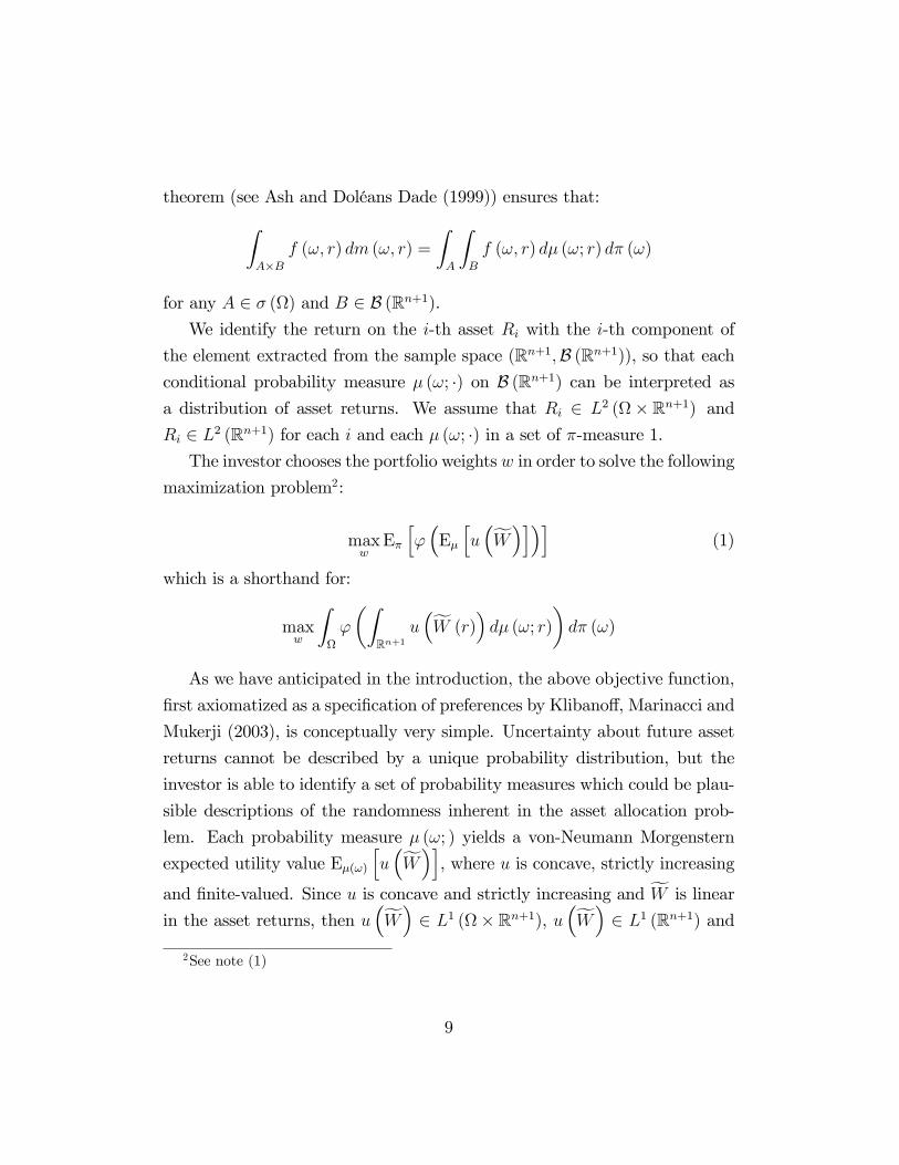
theorem (see Ash and Doléans Dade (1999)) ensures that:ZA�B

f (!; r) dm (!; r) =

ZA

ZB

f (!; r) d� (!; r) d� (!)

for any A 2 � () and B 2 B (Rn+1).We identify the return on the i-th asset Ri with the i-th component of

the element extracted from the sample space (Rn+1;B (Rn+1)), so that eachconditional probability measure � (!; �) on B (Rn+1) can be interpreted asa distribution of asset returns. We assume that Ri 2 L2 (� Rn+1) andRi 2 L2 (Rn+1) for each i and each � (!; �) in a set of �-measure 1.The investor chooses the portfolio weights w in order to solve the following

maximization problem2:

maxwE�h'�E�hu�fW�i�i (1)

which is a shorthand for:

maxw

Z

'

�ZRn+1

u�fW (r)

�d� (!; r)

�d� (!)

As we have anticipated in the introduction, the above objective function,

�rst axiomatized as a speci�cation of preferences by Klibano¤, Marinacci and

Mukerji (2003), is conceptually very simple. Uncertainty about future asset

returns cannot be described by a unique probability distribution, but the

investor is able to identify a set of probability measures which could be plau-

sible descriptions of the randomness inherent in the asset allocation prob-

lem. Each probability measure � (!; ) yields a von-Neumann Morgenstern

expected utility value E�(!)hu�fW�i, where u is concave, strictly increasing

and �nite-valued. Since u is concave and strictly increasing and fW is linear

in the asset returns, then u�fW� 2 L1 (� Rn+1), u�fW� 2 L1 (Rn+1) and

2See note (1)

9

E�(!)hu�fW�i is a � ()-measurable function belonging to L1 (). By con-

sidering all the probability measures � (!; �) for ! in , we obtain a wholerange of expected utility values; formally, we have a mapping U : ! Rde�ned by:

U (!) = E�(!)hu�fW�i

The investor subjectively assigns a degree of likelihood to the probability

measures � (!; �) , that is she forms a subjective measure �, assigning a prob-ability to a �-algebra � () of subsets of . This is compatible, for example,

with a Bayesian framework in which the distribution of asset returns is para-

metrized by a vector � and the investor assigns a non-degenerate probability

distribution to the parameter vector �.

Since U (!) is a measurable function and belongs to L1 (), the investor

is able to evaluate the integral:

E� [' (U)]

where ' is again taken to be a concave, strictly increasing and �nite-valued

function. The above expectation is an "expected utility of expected utili-

ties": if � is non-degenerate, the expected utility U is a random variable; the

investor, instead of simply maximizing the expected value E� [U ] of the possi-

ble values of U , maximizes the expectation E� [' (U)] of a concave transform

of U . By doing so, she incorporates ambiguity aversion into her objective

function: this is a consequence of the fact that by Jensen�s inequality:

E� [' (U)] � ' (E� [U ])

so that a setting in wich the expected utility of wealth is equal to E� [U ] with-

out ambiguity is preferred to one in which the expectation of the expected

utility of wealth has got the same value, but some ambiguity is present.

If the maximization problem (1) has got an interior solution and if both

10

u and ' are di¤erentiable, the following �rst order necessary condition must

be satis�ed:

E�h'0�E�hu�fW�i�E� hu0 �fW��R��!1 Rn+1�ii = 0 (2)

where we have assumed that di¤erentiation under the integral sign is legiti-

mate and the dominated convergence theorem applies: for example it su¢ ces

to assume that u0�fW� is bounded � (!; �)-a.s. for any ! in a set of �-measure

1 and '0�E�(!)

hu�fW�i� is bounded �-a.s.

It is worth commenting brie�y on this necessary condition: when there is

no ambiguity it simpli�es to

E�hu0�fW��R��!1 Rn+1�i = 0 (3)

which has a simple economic interpretation: if the portfolio allocation is

optimal, the marginal increase in utility obtained by selling one dollar worth

of asset n + 1 and investing the proceeds into any one of the other assets,

must have zero expected value. When ambiguity is present, i.e. � is non-

degenerate, condition (3) does not necessarily hold for every � (!; �); theremight be some probability measures � (!; �) under which a reallocation of theportfolio increases the expected utility value E�

hu�fW�i calculated under

those measures; however, once one accounts for the e¤ect of the reallocation

on the whole range of expected utility values, the overall marginal bene�t of

the reallocation must be zero.

Imposing very mild conditions on the structure of the problem (1), the

optimality condition (2) can be written in a form which is very similar to

(3). We state the result in the following proposition, which we prove in the

Appendix:

Proposition 1 Let ' and u be of class C1. Assume at an optimum u0�fW�

is bounded � (!; �)-a.s. for any ! in a set of �-measure 1 and '0�E�(!)

hu�fW�i�

11

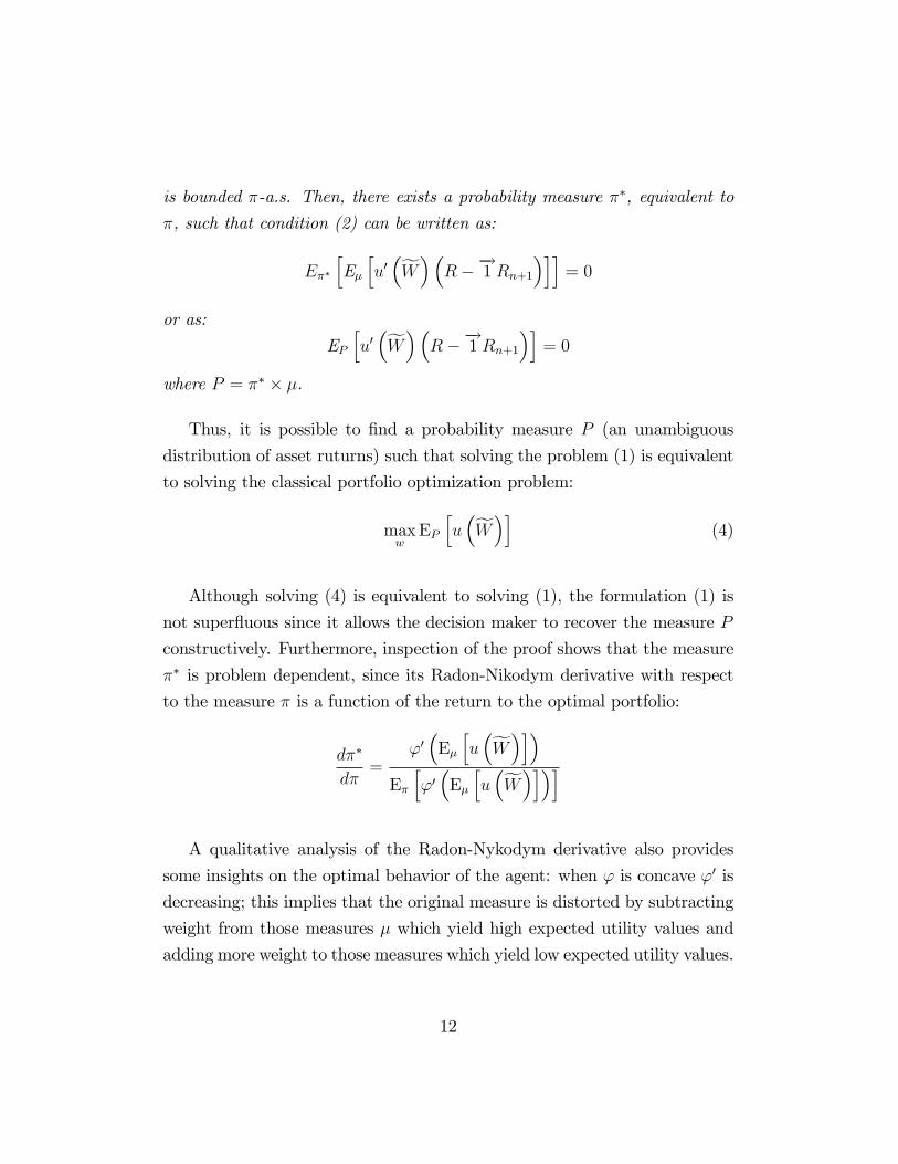
is bounded �-a.s. Then, there exists a probability measure ��, equivalent to

�, such that condition (2) can be written as:

E��hE�hu0�fW��R��!1 Rn+1�ii = 0

or as:

EPhu0�fW��R��!1 Rn+1�i = 0

where P = �� .

Thus, it is possible to �nd a probability measure P (an unambiguous

distribution of asset ruturns) such that solving the problem (1) is equivalent

to solving the classical portfolio optimization problem:

maxwEPhu�fW�i (4)

Although solving (4) is equivalent to solving (1), the formulation (1) is

not super�uous since it allows the decision maker to recover the measure P

constructively. Furthermore, inspection of the proof shows that the measure

�� is problem dependent, since its Radon-Nikodym derivative with respect

to the measure � is a function of the return to the optimal portfolio:

d��

d�=

'0�E�hu�fW�i�

E�h'0�E�hu�fW�i�i

A qualitative analysis of the Radon-Nykodym derivative also provides

some insights on the optimal behavior of the agent: when ' is concave '0 is

decreasing; this implies that the original measure is distorted by subtracting

weight from those measures � which yield high expected utility values and

adding more weight to those measures which yield low expected utility values.

12

In the next section we will analyse a special case in which, besides being

able to �nd closed formulas for the portfolio weights, we are able to derive

P explicitly.

2 A tractable case

To implement the model described in the previous section, one needs to

specify the functional forms of u and ' and the distributions � and �. We

propose a speci�cation which allows to derive the optimal portfolio weights

explicitly and gain some insight into the model. We �rst make the distri-

butional assumptions: for convenience, we specialize to the case in which

the (n + 1)-th asset is a risk-free asset, so that Rn+1 is equal to a constant

Rf ; we further assume that the vector R of returns is jointly normally dis-

tributed with E[R] = � and Var[R] = � (it will soon become clear why we

have chosen to assign the symbol � both to the expected return and to the

inner probability measure). However, the vector � of expected returns is not

known with certainty by the investor, who assigns the following distribution

to the parameter �:

� � N (m;S)

In the language of Bayesian statistics, this can be thought of as the prior

distribution of the parameter. Adopting the Bayesian perspective, the joint

distributional hypothesis on the parameter � and on the vector R can be

written as:

f (Rj�) = (2�)�n2 j�j�

12 exp

�(R� �)0��1 (R� �)

�(5)

f (�) = (2�)�n2 jSj�

12 exp

�(��m)0 S�1 (��m)

�As to the covariance matrix �, the fact that we assume that it is known

with certainty might seem unrealistic; however, this is not obviously so, since

it is often possible to sample the price processes generating the returns R at

13

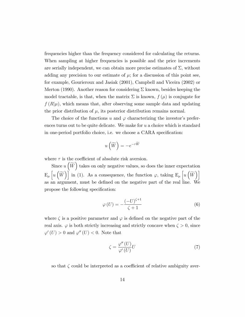
frequencies higher than the frequency considered for calculating the returns.

When sampling at higher frequencies is possible and the price increments

are serially independent, we can obtain more precise estimates of �, without

adding any precision to our estimate of �; for a discussion of this point see,

for example, Gourieroux and Jasiak (2001), Campbell and Viceira (2002) or

Merton (1990). Another reason for considering � known, besides keeping the

model tractable, is that, when the matrix � is known, f (�) is conjugate for

f (Rj�), which means that, after observing some sample data and updatingthe prior distribution of �, its posterior distribution remains normal.

The choice of the functions u and ' characterizing the investor�s prefer-

ences turns out to be quite delicate. We make for u a choice which is standard

in one-period portfolio choice, i.e. we choose a CARA speci�cation:

u�fW� = �e��fW

where � is the coe¢ cient of absolute risk aversion.

Since u�fW� takes on only negative values, so does the inner expectation

E�hu�fW�i in (1). As a consequence, the function ', taking E� hu�fW�i

as an argument, must be de�ned on the negative part of the real line. We

propose the following speci�cation:

' (U) = �(�U)�+1

� + 1(6)

where � is a positive parameter and ' is de�ned on the negative part of the

real axis. ' is both strictly increasing and strictly concave when � > 0, since

'0 (U) > 0 and '00 (U) < 0. Note that

� ='00 (U)

'0 (U)U (7)

so that � could be interpreted as a coe¢ cient of relative ambiguity aver-

14

sion, akin to an Arrow and Pratt�s coe¢ cient of relative risk aversion; note,

however, that, when compared to an Arrow and Pratt�s coe¢ cient, a minus

sign is missing in front of the right hand side of (7): the reason is that U

here is negative, while in the standard de�nition it is positive.

To gain a better understanding of the speci�cation of ', (6) can be written

as:

' (U) =(� (U))1�(�+2)

1� (� + 2)

� (U) = � 1U

� is a strictly monotone transformation and when U ranges in the interval

(�1; 0), � (U) takes values in the interval (0;1). Once this monotone trans-formation is accomplished, the � values are retransformed with a standard

power function with coe¢ cient � + 2. Roughly speaking, the choice of � + 2

as an exponent instead of � is just a concavity adjustment done to keep the

coe¢ cent of relative ambiguity aversion equal to �. Mapping utility values

from the interval (�1; 0) to the interval (0;1) via the � function also allowsus to switch from a scale of measurement ((�1; 0)) which does not possessan absolute zero, to a scale ((0;1)) which does: this is extremely impor-tant since de�ning relative ambiguity aversion calls for a relative scale and a

relative scale is well-de�ned only when an absolute zero can be identi�ed.

Another feature of the proposed speci�cation of ' about which it is worth

commenting is that when � = 0 the objective function reduces to:

E�hE�hu�fW�ii

i.e. to the case in which the investor simply averages over expected utility

values, so that this speci�cation also encompasses the case of no aversion

to ambiguity. This is equivalent to a Von-Neumann Morgenstern expected

utility where integration is with respect to the predictive distribution of the

15

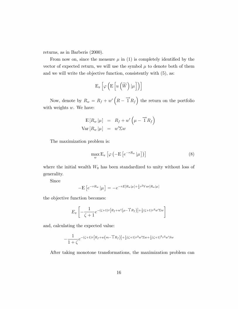
returns, as in Barberis (2000).

From now on, since the measure � in (1) is completely identi�ed by the

vector of expected return, we will use the symbol � to denote both of them

and we will write the objective function, consistently with (5), as:

E�h'�Ehu�fW� j�i�i

Now, denote by Rw = Rf + w0�R��!1 Rf

�the return on the portfolio

with weights w. We have:

E [Rw j� ] = Rf + w0��!1 Rf

�Var [Rw j� ] = w0�w

The maximization problem is:

maxwE��'��E

�e��Rw j�

��(8)

where the initial wealth W0 has been standardized to unity without loss of

generality.

Since

�E�e��Rw j�

�= �e��E[Rwj� ]+ 1

2�2V ar[Rwj� ]

the objective function becomes:

E�

�� 1

� + 1e�(�+1)�[Rf+w

0(��!1 Rf)]+ 1

2(�+1)�2w0�w

�and, calculating the expected value:

� 1

1 + �e�(�+1)�[Rf+w(m�

�!1 Rf)]+ 1

2(�+1)�2w0�w+ 1

2(�+1)2�2w0Sw

After taking monotone transformations, the maximization problem can

16

be rewritten as:

maxwRf + w

0�m��!1 Rf

�� 12�w0�w � 1

2(� + 1) �w0Sw

The �rst order condition is:

m��!1 Rf � ��w � (� + 1) �Sw = 0

which yields the optimal portfolio weights:

w� =1

�[� + (1 + �)S]�1

�m��!1 Rf

�(9)

The above formula for the optimal portfolio weights is better understood

when compared to the formula that arises in the case where parameter un-

certainty is not taken into account by the decision maker. Suppose that the

investor solves the standard optimization problem

maxw�E

�e��Rw

�(10)

disregarding the fact that the distribution of � is non-degenerate and setting

� = m: the optimal portfolio weights would be:

w�� =1

��1

�m��!1 Rf

�(11)

The optimal portfolio (9) di¤ers from (11) only for the fact that the matrix

(1 + �)S has been added to the covariance matrix �. According to Propo-

sition 1, we have been able to �nd an unambiguous distribution of asset

returns (a measure P ) such that solving (4) is equivalent to solving (1); such

a distribution is:

R � N (m;� + (1 + �)S)

To gain some intuition about the correction thus made to the variance

17

covariance matrix and to the portfolio weights, consider the case in which

� and S are diagonal (there is no covariance between asset returns and no

covariance between the parameters). If parameter uncertainty is not taken

into account the optimal weight given to a generic asset i is:

w��i =1

�

mi �Rf�2i

(12)

where wi is the weight of asset i in the optimal portfolio and mi and �2i are

the mean and the variance of the gross return on asset i. The weight is pro-

portional to the expected return in excess of the risk-free rate and inversely

proportional to the variance of the return; the coe¢ cient of proportionality

is the risk tolerance parameter 1�.

When parameter uncertainty is taken into account, the optimal weight

given to asset i is:

w�i =1

�

mi �Rf�2i + (1 + �) s

2i

(13)

where s2i is the variance of the parameter �i. Compared to the previous case,

the portfolio weight is reduced when there is parameter uncertainty (s2i is

positive) and the higher the ambiguity aversion coe¢ cient �, the greater this

reduction is. This result is in accordance with Uppal and Wang�s (2003)

�ndings: although their portfolio selection model is dynamic and set in con-

tinuous time, it is comparable to ours because they also assume that the only

ambiguity is about expected returns (drifts); in their model all the proba-

bility measures can be recovered from each other via a Girsanov change of

measure, hence leaving the volatility unchanged. What they �nd is that in

the presence of ambiguity and with a preference for robustness, the weight

given to an ambiguous asset is smaller than the weight that would be given to

the same asset in a traditional intertemporal Merton model; the role played

in our model by the coe¢ cient of ambiguity aversion is akin to the role played

in their model by the degree of con�dence in the reference measure.

Resorting to results from matrix perturbation theory, one can also do

18

some comparative statics on the unconditional expected return and the un-

conditional variance of the optimal portfolio.

Note that the �rst two unconditional moments of the return on the opti-

mal portfolio are:

E [Rw� ] = Rf + w�0�m��!1 Rf

�Var [Rw� ] = E [Var [Rw� j� ]] +Var [E [Rw� j� ]] = w�0 (� + S)w�

The sensitivity of the two above moments to changes in the ambiguity aver-

sion coe¢ cient � is characterized by the following proposition:

Proposition 2 Let Rw� be the return on the optimal portfolio, selected ac-cording to the rule (9). Then the unconditional expected return E[Rw� ] on

the optimal portfolio is a decreasing function of the coe¢ cient of ambiguity

aversion �. Furthermore, its derivative is:

@E [Rw� ]

@�= �1

�

nXi=1

nXj=1

1

�i�ju0iSuju

0j

�m��!1 Rf

��m��!1 Rf

�0ui

where �i and ui are the eigenvalues and the eigenvectors of the matrix A =

� + (1 + �)S. In the special case in which � = 0 also the unconditional

variance of the return on the optimal portfolio is a locally decreasing function

of � and:@Var [Rw� ]

@�=1

�

@E [Rw� ]@�

We have not been able to �nd the derivative of Var[Rw� ] for the more

general case in which � 6= 0. Furthermore, we would like to be able to saysomething about the impact of introducing (or increasing) ambiguity aversion

on the e¢ ciency of the portfolios selected by the investor, for example by

examining the behavior of the Sharpe ratio:

Sh (Rw) =E [Rw]�RfpVar [Rw]

19

For this reason we have conducted some simulations (whose results are

commented in the next section) to understand more about the comparative

statics of the optimal portfolio.

3 Empirical results

In this section we conduct an empirical analysis of the portfolio allocation

rule proposed in the previous section.

We assume that returns are generated according to (5). R is taken to

be a vector of monthly returns on 30 stocks. The covariance matrix � is

set equal to the sample covariance matrix of the monthly returns on the 30

stocks included in the Dow Jones Industrial Average Index, calculated from

a sample of 120 monthly returns (January 1994 to December 2003).

We impose the following structure on m and S:

m = m�!1 (14)

S = s2I + c��!1�!1 0 � I

�where m, s and c are scalars and c is constrained to lie in the open interval�� s2

n�1 ; s2�to ensure that S is positive de�nite (we include in the Appendix a

proof of the fact that this condition is both necessary and su¢ cient). Thus,

we require that both the expectation and the variance of the parameters

�i are equal across assets; we also require that all the covariances between

the parameters are equal. This is the same structure assumed by Frost and

Savarino (1986), although in a slightly di¤erent setting. It has the advantage

that by varying a single parameter (c) one is able to analyse the impact of a

change in the covariance structure on the portfolio statistics. We will later

deal with a more general structure.

As a �rst step, a reference model is de�ned by choosing a particular set

of values for the parameters. We set � = 10, � = 2, m = 1+0:5%, s = 0:3%,

20

pc = 0:1% and Rf = 1+0:2% (note that the returns are monthly returns and

the optimization horizon is the month). Comparative statics are performed

by varying one parameter at a time over a range of values. The �gures in

the Appendix report the results of this exercise, displaying the impact of

changing the parameters on the unconditional expected return E[Rw� ], on

the unconditional standard deviation Sd[Rw� ] =pVar [Rw� ], on the Sharpe

ratio Sh[Rw� ] and on the sum of absolute portfolio weights:

a =30Xi=1

jwij

Increasing the coe¢ cient of ambiguity aversion � decreases the expected

return (as predicted by Proposition 2) and the standard deviation. Also the

Sharpe ratio slightly declines, while the sum of absolute portfolio weights

decreases substantially. Increasing s or c seems to produce the same e¤ect

as an increase in �. Hence, an increase in ambiguity or in ambiguity aversion

induces the investor to form a less aggressive portfolio of risky assets (as re-

�ected in the fact that the sum of absolute portfolio weights diminishes), with

the consequence that both the expected return and the standard deviation

of the portfolio are reduced.

Since the results presented so far could depend on the fact that we have

assumed a very particular structure for m and S, we perform some simula-

tions in which m and S assume a di¤erent structure. Roughly speaking, the

idea behind the simulations is to take a prior as in (14), generate consistently

a parameter � at each simulation, then generate a path of asset returns and

update the prior based on the observed sample, thus losing the structure

(14).

We perform four sets of 100,000 simulations: a �rst set is performed with

the reference parameters detailed above and three more sets are performed

choosing di¤erent values for m, s and c, as reported in the tables in the

Appendix.

21

We start each simulation by randomly generating a value for �, drawn

from the distribution with density

f (�) = (2�)�n2 jSj�

12 exp

�(��m)0 S�1 (��m)

�Conditioning on this value of �, we simulate a sample of 24 monthly

returns fRt; t = 1; : : : ; 24g, generated independently from the distribution

with density

f (Rtj�) = (2�)�n2 j�j�

12 exp

�(Rt � �)0��1 (Rt � �)

�and we use the returns thus simulated to update the prior distribution ac-

cording to the Bayesian updating formulas:

f (�jR1; : : : ; R24) = (2�)�n2 jS1j�

12 exp

�(��m1)

0 S�11 (��m1)�

where

m1 =�S�1 + 24��1

��1 �S�1m+ 24 � ��1R

�S1 =

�S�1 + 24 � ��1

��1and R is the sample average of the returns Rt.

After updating the prior, we use it to calculate the optimal portfolio w�

which solves the maximization problem (8):

w� = w��R�=1

�[� + (1 + �)S1]

�1�m1 �

�!1 Rf

�where the notation w

�R�has been chosen to emphasize the dependence of

the optimal portfolio on the observed average returns.

We calculate the conditional expected return on the portfolio:

E [Rw�j�] = w�0��!1 Rf

�+Rf

22

its conditional variance:

Var [Rw�j�] = w�0�w�

and the sum of absolute portfolio weights. All the above quantities are calcu-

lated conditioning on the true value of �, which is not known to the investor

and they are calculated repeatedly, changing the value of the ambiguity aver-

sion coe¢ cient � . We report in the Appendix the results obtained when �

takes values in the set f0; 2; 4; 8; 16; 32g. We report also the results obtainedfollowing the standard asset allocation rule:

w�� = ��1�m1 �

�!1 Rf

�This is, for example, the rule followed by Frost and Savarino (1986), with

the di¤erence that in their simulation exercise � is unknown and they use a

Normal-Wishart prior on (�;�).

We also include in the tables a measure of the distance of the selected

portfolio from the frontier of e¢ cient portfolios. Note that ex-post (when �

is perfectly known) all minimum variance portfolios have a stock component

which is a scalar multiple of the portfolio:

w�� = ��1��!1 Rf

�We propose to measure the distance of a generic portfolio w from the frontier

of minimum variance portfolios as

� (w) = min�kw � �w��k2 (15)

where � is a scalar and kk2 is the Euclidean norm. The e¢ cient portfo-lio ��w�� which solves the above minimum norm problem is the orthogonal

23

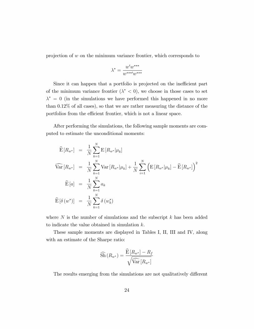
projection of w on the minimum variance frontier, which corresponds to

�� =w0w��

w��0w��

Since it can happen that a portfolio is projected on the ine¢ cient part

of the minimum variance frontier (�� < 0), we choose in those cases to set

�� = 0 (in the simulations we have performed this happened in no more

than 0.12% of all cases), so that we are rather measuring the distance of the

portfolios from the e¢ cient frontier, which is not a linear space.

After performing the simulations, the following sample moments are com-

puted to estimate the unconditional moments:

bE [Rw� ] = 1

N

NXk=1

E [Rw�j�k]

dVar [Rw� ] = 1

N

NXk=1

Var [Rw�j�k] +1

N

NXi=1

�E [Rw�j�k]� bE [Rw� ]�2

bE [a] = 1

N

NXk=1

ak

bE [� (w�)] = 1

N

NXk=1

� (w�k)

where N is the number of simulations and the subscript k has been added

to indicate the value obtained in simulation k.

These sample moments are displayed in Tables I, II, III and IV, along

with an estimate of the Sharpe ratio:

cSh (Rw�) = bE [Rw� ]�RfqdVar [Rw� ]The results emerging from the simulations are not qualitatively di¤erent

24

from those that emerged from the previous simpler comparative statics ex-

ercises: the more the ambiguity aversion coe¢ cient � is increased, the less

aggressive the portfolio is; increasing � leads to a reduction of the expected

return, of the standard deviation of returns and of the sum of absolute port-

folio weights. A novel feature is that, when � is increased, the Sharpe ratio

remains virtually unchanged, but the average distance from the e¢ cient fron-

tier diminishes, so that these two measures provide con�icting evidence on

the e¤ect of increased ambiguity aversion on portfolio e¢ ciency: while the

behavior of the Sharpe ratio would suggest that more ambiguity aversion

does not lead to improvements in e¢ ciency, the diminishing distance from

the e¢ cient frontier seems to be a sign of improved robustness. The im-

pact on portfolio statistics of switching from a traditional portfolio rule to

the portfolio rule we propose is similar to the impact just described of an

increase in ambiguity aversion.

Table V reports some features of the empirical distribution of the condi-

tional expected return on the optimal portfolio: the expected return E[Rw�j�]is itself a random variable, being a function of the parameter � and of the

portfolio selected, and hence it takes a di¤erent value at each simulation, giv-

ing rise to an empirical distribution of conditional expected returns, which

approximates the true distribution. The standard deviation of this distribu-

tion decreases as the coe¢ cient of ambiguity aversion increases, so that more

ambiguity aversion leads to a less volatile conditional expected return across

scenarios. It is also interesting that the �rst percentile of the distribution

increases when the coe¢ cient of ambiguity aversion increases: this means

that, although the unconditional expected return is lower when ambiguity

aversion is increased, so that the distribution of conditional expected returns

is shifted to the left, its left tail (comprising those cases in which the condi-

tional expected return of the portfolio is disappointingly low), is considerably

shortened and moved to the right.

25

4 Conclusions

We have addressed the problem of optimally selecting a portfolio of assets

when the probabilistic distribution of asset returns is not known with preci-

sion. Many researchers argue that standard portfolio allocation rules are not

robust, in the sense that even slight departures from the true distribution of

asset returns may lead to select portfolios that are far from being optimal.

We have proposed a model which allows to incorporate individual attitudes

towards ambiguity (uncertainty about the true distribution of asset returns)

into the portfolio selection process: we have done this by using a speci�-

cation of preferences which to our knowledge has never been used in asset

allocation models and which allows to easily parametrize both risk aversion

and aversion to ambiguity.

We have fully analysed a special case of our model where we are able

to explicitly derive the optimal portfolio weights when expected returns are

uncertain. This is in a sense complementary to a recent work by Jagannathan

and Ma (2003) which deals with uncertainty about the covariance matrix of

returns.

Our model has both normative and positive implications: besides giving

a portfolio allocation rule, it yields sharp predictions about the behavior of

an ambiguity averse individual; an ambiguity averse individual reduces her

position in those assets whose expected returns are uncertain and the greater

the uncertainty and the aversion to uncertainty, the greater the reduction is.

We have conducted some simulations to gain a better understanding of

the implications of our portfolio rule. Each time an investor is confronted

with a di¤erent data set to estimate the same distribution of asset returns,

he chooses a di¤erent portfolio, with a di¤erent expected return: with our

allocation rule the variability of portfolio expected returns seems to be lower

than with a standard allocation rule.

Although we have thoroughly investigated only a tractable case, the

framework set up in the paper is general enough to leave space for further

26

research: a possible direction of future e¤orts could be to �nd an allocation

rule for the more general case in which both the means and the variances of

asset returns are uncertain and to understand the interaction between these

two kinds of ambiguity.

27

References

[1] Anderson, E. W., L. P. Hansen and T. J. Sargent, 2003, "A Quartet

of Semigroups for Model Speci�cation, Robustness, Prices of Risk and

Model Detection", Journal of the European Economic Association, 1,

68-123.

[2] Ash, R. and C. Doléans-Dade, 1999, Probability and Measure Theory,

Harcourt Academic Press, San Diego.

[3] Barberis, N., 2000, "Investing for the Long Run when Returns are Pre-

dictable", Journal of Finance, 55, 225-264.

[4] Barry, C. B., 1974, "Portfolio Analysis under Uncertain Mean, Variances

and Covariances", Journal of Finance, 29, 515-522.

[5] Bawa, V. S. and R. W. Klein, 1976, "The E¤ect of Estimation Risk on

Optimal Portfolio Choice", Journal of Financial Economics, 3, 215-231.

[6] Becker B., W. Marty and B. Rustem, 2000, "Robust Min-Max Portfolio

Strategies for Rival Forecast and Risk Scenarios", Journal of Economic

Dynamics and Control, 24, 1591-1621.

[7] Black, F. and R. Litterman, 1992, "Global Portfolio Optimization", Fi-

nancial Analyst Journal, 48, 28-43.

[8] van Bossum, M. A., 2002, Semide�nite Optimization, a Spectral Ap-

proach, unpublished PhD Dissertation, University of Utrecht.

[9] Campbell, J. Y. and L. M. Viceira, 2002, Strategic asset allocation,

Oxford University Press, New York.

[10] Chen, Z. and L. Epstein, 2002, "Ambiguity, Risk and Asset Returns in

Continuous Time", Econometrica, 70, 1403-1443.

28

[11] Dow, J. and S. R. da Costa Werlang, 1992, "Uncertainty Aversion, Risk

Aversion and the Optimal Choice of Portfolio", Econometrica, 60, 197-

204.

[12] Ellsberg, D., 1961, "Risk, Ambiguity and the Savage Axioms", Quarterly

Journal of Economics, 75, 643-669.

[13] Epstein, L. and T. Wang, 1994, "Intertemporal Asset Pricing under

Knightian Uncertainty", Econometrica, 62, 283-322.

[14] Frankfurter, G. M., H. E. Phillips and J. P. Seagle, 1971, "Portfolio

Selection: The E¤ect of Uncertain Mean, Variances and Covariances",

Journal of Financial and Quantitative Analysis, 6, 1251-1262.

[15] Frost, P. A. and J. Savarino, 1988, "An Empirical Bayes Approach

to E¢ cient Portfolio Selection", Journal of Financial and Quantitative

Analysis, 21, 293-305.

[16] Gourieroux, C. and J. Jasiak, 2001, Financial econometrics: problems,

models and methods, Princeton University Press, Princeton.

[17] Green, R. C. and B. Holli�eld, 1992, "When will Mean-Variance E¢ cient

Portfolios be Well Diversi�ed?", Journal of Finance, 47, 1785-1809.

[18] Jagannathan, R. and T. Ma, 2003, "Risk Reduction in Large Portfolios

- Why Imposing the Wrong Constraints Helps", Journal of Finance, 58,

1651-1684.

[19] Jobson, J. D. and B. Korkie, 1980, "Estimation for Markowitz E¢ cient

Portfolios", Journal of the American Statistical Association, 75, 544-554.

[20] Klibano¤, P., M. Marinacci and S. Mukerji, 2003, "A smooth model of

decision making under ambiguity", ICER Working Paper no. 11/2003.

[21] Knight, F. H., 1921, Risk, Uncertainty and Pro�t, Houghton Mi in,

Boston.

29

[22] Krasker, W. S., 1982, "Minimax Behavior in Portfolio Selection", Jour-

nal of Finance, 37, 609-614.

[23] Lucas, R. E., 1978, "Asset Prices in an Exchange Economy", Economet-

rica, 46, 1429-1445.

[24] Maenhout, P. J., 2004, "Robust Portfolio Rules and Asset Pricing",

forthcoming in Review of Financial Studies.

[25] Markowitz, H. M., 1952, "Portfolio Selection", Journal of Finance, 7,

77-91.

[26] Merton, R. C., 1990, Continuous time �nance, Basil Blackwell, Cam-

bridge.

[27] Savage, L. J., 1954, The Foundations of Statistics, John Wiley and Sons,

New York.

[28] Torki, M., 2001, "Second-order Directional Derivatives of all Eigenval-

ues of a Symmetric Matrix", Nonlinear Analysis, Theory, Methods and

Applications, 46, 1133-1150.

[29] Uppal, R. and T. Wang, 2003, "Model Misspeci�cation and Underdiver-

si�cation", Journal of Finance, 58, 2465-2486.

30

Appendix

Proof of Proposition 1. The optimality condition is:

E�h'0�E�hu�fW�i�E� hu0 �fW��R��!1 Rn+1�ii = 0

where u0�fW� is bounded � (!; �)-a.s. for any ! in a set of �-measure 1 and

'0�E�(!)

hu�fW�i� is bounded �-a.s.

Under the assumptions stated in Section 1, E�hu�fW�i is � ()-measurable;

furthermore, '0 is continuous since ' 2 C1, hence '0�E�hu�fW�i� is � ()-

measurable; it is also strictly positive. De�ne:

� ='0�E�hu�fW�i�

E�h'0�E�hu�fW�i�i

where the denominator is �nite given the boundedness assumption on '0�E�(!)

hu�fW�i�.

The optimality condition can be rewritten as:

E�h�E�

hu0�fW��R��!1 Rn+1�ii = 0

Since � > 0 and E� [�] = 1, � can be used to de�ne a change of measure

and write the optimality condition as:

E��hE�hu0�fW��R��!1 Rn+1�ii = 0

where �� is another probability measure, absolutely continuous with respect

to �, with Radon-Nikodym derivative

d��

d�= �

31

The above double expectation is just a double integral:Z

ZRnu0�fW��R��!1 Rn+1� d� (!; r) d�� (!)

Since u0�fW� is bounded � (!; �)-a.s. for any ! in a set of �-measure 1

and Ri 2 L2 (Rn) for any i, the inner integral belongs to L1 (), Tonelli�stheorem guarantees that the integralZ

�Rnu0�fW��R��!1 Rn+1� d�� (!; r)

is well-de�ned and equals the above double integral.

Thus, the optimality condition becomes:

EPhu0�fW��R��!1 Rn+1�i = 0

where P = �� .

32

Proof of Proposition 2. To prove this proposition we will need the

following lemma, which can be found in van Bossum (2002) and descends

from a more general theorem in Torki (2001).

Lemma 3 : let A be a symmetric and positive de�nite (n� n) matrix whichcan be written as:

A = y1B1 + y2B2 + : : :+ ykBk

where B1, B2,..., Bk are positive semide�nite matrices and y1, y2,..., yk are

positive scalars. Let A have n distinct eigenvalues �1, �2,..., �n (they are real

and strictly positive) and denote by u1, u2,..., un their respective eigenvectors

(chosen so as to be orthonormal). Then:

@�i@yj

= u0iBjui

@2�i@yl@yj

= 2Xr 6=i

u0iBluru0iBjur

�i � �r

De�ne

A (�; t) = � + (1 + �)S + tzz0

where z = m��!1 Rf .

We can diagonalize A (�; 0) as follows:

A (�; 0) = U�U 0

where U is the matrix whose columns u1, u2,..., un are the orthonormal

eigenvectors of A (�; 0) and � is the diagonal matrix of eigenvalues.

The expected return on the optimal portfolio can be written as:

E [Rw� ] =1

�z0U��1U 0z +Rf

33

Expanding the product:

�E [Rw� ] =z0u1u

01z

�1+z0u2u

02z

�2+ : : :+

z0unu0nz

�n+ �Rf

or:

�E [Rw� ] =u01zz

0u1�1

+u02zz

0u2�2

+ : : :+u0nzz

0un�n

+ �Rf

which, applying the above lemma, becomes:

�E [Rw� ] =nXi=1

1

�i

@�i@t+ �Rf

Taking the derivative with respect to �, we get:

�@E [Rw� ]

@�=

nXi=1

1

�i

@2�i@�@t

�nXi=1

1

�2i

@�i@t

@�i@�

=

=

nXi=1

1

�i

"2Xj 6=i

u0iSuju0izz

0uj�i � �j

� u0iSuiu

0izz

0ui�i

#

Setting Qij = u0iSuju0jzz

0ui and noting that Qij = Qji, we can write:

�@E [Rw� ]

@�=

nXi=1

"2i�1Xj=1

�Qij

�i (�i � �j)+

Qji�j (�j � �i)

�� Qii�2i

#=

=nXi=1

"2i�1Xj=1

�(�j � �i)Qij�i�j (�i � �j)

�� Qii�2i

#=

= �nXi=1

nXj=1

Qij�i�j

Since the eigenvalues are strictly positive and the Qij are positive,

@E [Rw� ]

@�� 0

34

The second part of the proposition is easily proved by noting that:

Var [Rw� ] = w�0 (� + S)w� =1

� 2z0 [� + (1 + �)S]�1 (� + S) [� + (1 + �)S]�1 z

When � = 0 it simpli�es to:

Var [Rw] = w�0 (� + S)w� =1

� 2z0 [� + S]�1 z =

1

�(E [Rw]�Rf )

so that:@Var [Rw� ]

@�=1

�

@E [Rw� ]@�

35

Upper and lower bounds on c. Deriving upper and lower bounds for c

is an easy task, once one makes use of the following:

Lemma 4 Lemma: if A is a (n� n) matrix with eigenvalues �1, �2,. . . , �n

and � is a scalar, then the eigenvalues of the matrix A + �I are �1 + �,

�2 + �,. . . , �n + �.

The eigenvalues of the (n� n) matrix �!1 �!1 0 are �1 = n, �2 = 0,. . . ,

�n = 0. This is easily seen by noting that the rank of�!1�!1 0 is 1, so that

n � 1 of its eigenvalues must be zero, and n is an eigenvalue associated tothe eigenvector

�!1 .

By the above lemma, the eigenvalues of the matrix

S =�s2 � c

�I + c

�!1�!1 0

are �1 = cn+ s2 � c, �2 = s2 � c,. . . , �n = s2 � c.The requirement that all the eigenvalues be strictly greater than zero

yields the two conditions:

c < s2

c > � s2

n� 1

36

Table 1Summary statistics of the portfolios

This table presents some summary statistics of the portfolios selected by an

ambiguity averse investor, according to the optimal rule described in the paper.bE [Rw� ] is the Monte Carlo estimate of the unconditional monthly expected re-turn on the portfolio, cSd [Rw�j�] estimates the standard deviation, cSh [Rw�j�]the Sharpe ratio, bE [� (w�)] the expected distance of the portfolio from the truly

e¢ cient frontier and bE [a] the expected value of the sum of absolute portfolio

weights. All the values displayed in the table are averages, calculated from a

sample of 100,000 simulations and conditioning on the true value of the vector

of expected returns �, which is not known to the investor (the ambiguity in the

model is about �). The table contains the statistics relative to six di¤erent port-

folios (corresponding to di¤erent values of the ambiguity aversion coe¢ cient �)

plus a seventh portfolio, marked with a (*), chosen by an investor who disregards

ambiguity and adopts a standard portfolio selection rule. The vector of monthly

expected returns � is drawn at each simulation from a multivariate normal distri-

bution, with E[�] = m�!1 and Var[�] = s2I+ c

��!1�!1 0 � I

�. In the present table

m� 1 = 0:5%, s = 0:3% andpc = 0:1%. The net riskfree rate of return is set

equal to 0.2% and the coe¢ cient of absolute risk aversion is � = 10.

m� 1 = 0:5% s = 0:3%pc = 0:1%

� bE [Rw� ] cSd [Rw� ] cSh [Rw� ] bE [� (w�)] bE [a]* 0.3716% 1.3154% 0.1304 0.2570 1.2049

0 0.3708% 1.3097% 0.1304 0.2554 1.1977

2 0.3694% 1.2984% 0.1304 0.2524 1.1835

4 0.3679% 1.2874% 0.1304 0.2494 1.1696

8 0.3651% 1.2662% 0.1304 0.2436 1.1430

16 0.3599% 1.2270% 0.1303 0.2330 1.0937

32 0.3507% 1.1589% 0.1301 0.2145 1.0081

37














��!1�!1 0 � I


m�1 = 0:7%, s = 0:2% andpc = 0. The net riskfree rate of return is set equal

to 0.2% and the coe¢ cient of absolute risk aversion is � = 10.

m� 1 = 0:7% s = 0:2%pc = 0


0 0.4613% 1.6155% 0.1617 0.2505 1.2166

2 0.4605% 1.6107% 0.1617 0.2489 1.2091

4 0.4597% 1.6060% 0.1617 0.2474 1.2017

8 0.4582% 1.5967% 0.1617 0.2443 1.1872

16 0.4553% 1.5792% 0.1616 0.2385 1.1595

32 0.4499% 1.5471% 0.1615 0.2278 1.1088

38














��!1�!1 0 � I


m� 1 = 0:3%, s = 0:4% andpc = 0:3%. The net riskfree rate of return is set


m� 1 = 0:3% s = 0:4%pc = 0:3%


0 0.2962% 0.9854% 0.0976 0.2127 0.9895

2 0.2950% 0.9731% 0.0976 0.2100 0.9772

4 0.2938% 0.9612% 0.0976 0.2074 0.9652

8 0.2916% 0.9384% 0.0976 0.2024 0.9423

16 0.2875% 0.8968% 0.0976 0.1932 0.9002

32 0.2805% 0.8260% 0.0974 0.1774 0.8281

39














��!1�!1 0 � I


m � 1 = 0:5%, s = 1% andpc = 0:8%. The net riskfree rate of return is set


m� 1 = 0:5% s = 1%pc = 0:8%


0 1.8724% 4.1980% 0.3983 0.7046 4.0299

2 1.8121% 4.0446% 0.3985 0.6789 3.8849

4 1.7564% 3.9038% 0.3986 0.6552 3.7511

8 1.6568% 3.6539% 0.3987 0.6131 3.5121

16 1.4945% 3.2499% 0.3983 0.5448 3.1219

32 1.2639% 2.6826% 0.3965 0.4482 2.5673

40

Table 5Empirical distribution of the expected rate of return

This table displays some features of the empirical distribution of the monthly

conditional expected return E[Rw�j�] on the portfolios selected by an ambiguityaverse investor, according to the optimal rule described in the paper. E[Rw�j�]depends on the portfolio selected by the investor and on the realization of the

paramerer vector �; hence, we obtain a di¤erent value for each of the 100,000

simulations we perform, which gives rise to an empirical distribution of E[Rw�j�].We report both the standard deviation and some percentiles of the distribution.

Each row corresponds to a di¤erent value of the ambiguity aversion coe¢ cient �,

while the row marked with a (*) corresponds to the case in which the investor

disregards ambiguity and adopts a standard portfolio selection rule. The vector

of monthly expected returns � is drawn at each simulation from a multivariate

normal distribution, with E[�] = m�!1 and Var[�] = s2I + c

��!1�!1 0 � I

�. In the

present table m = 0:5%, s = 0:3% and c = 0:1%. The riskfree rate of return is

set equal to 0.2%.

Percentiles of the distributions

� Std deviation 1st 10th 20th 80th 90th 99th

* 0.1058% 0.168% 0.252% 0.285% 0.450% 0.507% 0.699%

0 0.1051% 0.168% 0.252% 0.285% 0.449% 0.506% 0.686%

2 0.1038% 0.169% 0.252% 0.284% 0.447% 0.503% 0.681%

4 0.1025% 0.170% 0.252% 0.284% 0.444% 0.500% 0.676%

8 0.1001% 0.172% 0.252% 0.283% 0.440% 0.494% 0.666%

16 0.0956% 0.175% 0.251% 0.281% 0.431% 0.483% 0.646%

32 0.0878% 0.180% 0.250% 0.278% 0.417% 0.464% 0.610%

41

Figure 1: The impact of an increase in ambiguity aversion. These plots depictthe impact of increasing the coe¢ cient of ambiguity aversion � on somestatistics describing the optimal portfolio (unconditional expected return,standard deviation, Sharpe ratio and average value of the sum of absoluteportfolio weights).

42

Figure 2: The impact of an increase in ambiguity. These plots depict theimpact of increasing the variance s of the unknown parameter on some statis-tics describing the optimal portfolio (unconditional expected return, standarddeviation, Sharpe ratio and average value of the sum of absolute portfolioweights).

43

Figure 3: The impact of an increase in the covariance between parameters.These plots depict the impact of increasing the covariance c between theunknown parameters on some statistics describing the optimal portfolio (un-conditional expected return, standard deviation, Sharpe ratio and averagevalue of the sum of absolute portfolio weights).

44

Documents

Munich Personal RePEc Archive - uni-muenchen.de · Traditional static portfolio selection models, such as Markowitz™s (1952), assume that the distribution of asset returns is objectively