MPRAMunich Personal RePEc Archive

Performance of Markov-SwitchingGARCH Model Forecasting InflationUncertainty

Tasneem Raihan

University of California, Riverside

31 October 2017

Online at https://mpra.ub.uni-muenchen.de/82343/MPRA Paper No. 82343, posted 1 November 2017 21:56 UTC

Performance of Markov-Switching GARCH Model

Forecasting Inflation Uncertainty

Tasneem Raihan

October 31, 2017

Abstract

This paper seeks to uncover the non-linear characteristics of uncertainty underlyingthe US inflation rates over the period 1971-2015 within a regime-switching framework.Accordingly, we employ two variants of a Markov regime-switching GARCH model,one with normally distributed errors (MS-GARCH-N) and another with t-distributederrors (MS-GARCH-t), and compare their relative in-sample as well as out-of-sampleperformances with those of their standard single-regime counterparts. Consistent withthe findings in existing studies, both of our regime-switching models are successfulin identifying the year 1984 as the breakpoint in inflation volatility. Among otherinteresting results is a new finding that the process of switching to the low volatilityregime started around April, 1979 and continued until mid 1983. This time frame ismatched with the period of aggressive monetary policy changes implemented by thethen Fed chairman Paul Volcker. As regards the performance in forecasting uncertainty,for shorter horizons spanning 1 to 5 months, MS-GARCH-N forecasts are found tooutperform all other models whereas for 8 to 12-month ahead forecasts MS-GARCH-tappears superior.

Key words: Markov-switching GARCH, inflation uncertainty, forecasting.JEL classification: E31, C01, C53.

1 Introduction

Uncertainties of various macroeconomic and financial variables have garnered special atten-

tion of both academic researchers and practitioners because of the nontrivial role they play

in influencing policy making and financial market decisions. For example, during the period

1979-1982, the Federal Reserve switched from targeting interest rates to using nonborrowed

reserves as a monetary policy tool which led to unprecedented interest rate volatility. This

rise in volatility might have distorted the relationship between nominal interest rates and

other explanatory variables which are important ingredients in the policy making process

(Gray, 1996). Another example of a macroeconomic variable which is susceptible to uncer-

tainty is exchange rate. Financial market exploits exchange rate’s volatility to determine the

price of currency options which in turn is used for risk management. It is not difficult to find

other variables that the portfolio managers, option traders and market makers all are inter-

ested in forecasting to either increase profit or hedge against risk. Hence, the importance of

an accurate estimation and forecast of volatility cannot be overstated.

Such forecasts typically hinge on the stylized facts that high frequency time series data

exhibit time-varying volatility and volatility clustering. The latter means that volatility

periods of similar magnitude tend to cluster together. To capture these features, the most

commonly used model in the literature is GARCH (Generalized Autoregressive Conditional

Heteroskedasticity) first introduced by Bollerslev (1986) who generalized the idea of ARCH

(Autoregressive Conditional Heteroskedasticity) by Engle (1982). Although GARCH models

produces a better fit than a constant variance model and also yields good volatility forecasts

as maintained by Andersen and Bollerslev (1998), there is a caveat. As Gray (1996) has

argued these models maybe misspecified due to the reason that the structural form of condi-

tional means and variances is relatively inflexible. In other words, the models are held fixed

throughout the entire sample period and thus ignore possible structural changes in mean and

variances. The latter may lead to estimated high persistence of individual shocks resulting in

high volatility persistence as shown by Lamoureux and Lastrapes (1990). This high volatility

persistence may be the reason behind excessive GARCH forecasts in volatile periods. To

1

solve this problem, researchers have recently generalized the GARCH model by allowing for

multiple regimes with varying volatility levels. This is called the Markov-Switching GARCH

(MS-GARCH) model.

The main objective of this paper is to examine the forecasting performance of a two-

regime MS-GARCH model with respect to inflation uncertainty in U.S over the period Jan-

uary 1971- March 2015 using multiple statistical loss functions. Performances of two variants

of an MS-GARCHmodel, one with normally distributed errors and another with t-distributed

errors are juxtaposed with the performances of their standard non-regime switching coun-

terparts. The existing literature so far has produced evidences on forecasting the volatility

of exchange rates and stock returns using MS-GARCH. But surprisingly, the performance

of MS-GARCH model forecasting inflation uncertainty has not been examined yet. It is

important to put MS-GARCH to test to see how well it performs while forecasting inflation

certainty for at least two reasons. First of all, it will shed light on the method’s appropriate

applicability in terms of forecasting. Second, inflation uncertainty is itself a very important

macroeconomic variable which affects a society’s welfare. It, in fact, was the first variable

modeled using ARCH (Engle, 1982, 1983).

As far as the first reason is concerned, obviously the same model cannot be expected

to be equally good in characterizing and forecasting different variables. Therefore, testing

MS-GARCH’s forecasting capability with respect to different variables will yield a better

understanding of the method’s usefulness. The appropriateness of the application of MS-

GARCH to inflation uncertainty can be primarily ascertained by eyeballing the data on

U.S. inflation rate from 1971 to early 2014 (Figure 1). It seems that inflation rate was

very volatile from early 1970s to mid 1980s. After that it remained relatively stable until

before 2006 which coincides with the onset of the recent financial crisis. Therefore, a casual

observation of the data suggests that the U.S. inflation rate might be characterized by at

two regimes: a high volatility regime and a low volatility regime. While a standard GARCH

model is not capable of distinguishing between these two regimes an MS-GARCH model is

better suited at this task.

2

Figure 1:

On the other hand, inflation uncertainty’s being a variable of great interest to many

parties is related to the general consensus that its future values are a major reason behind

the welfare loss associated with inflation. Engle (1983) has argued that inflation uncertainty

causes loss to risk averse economic agents even if the prices and quantities are perfectly

flexible in all markets. It also distorts the efficiency of the current period’s resource allocation

decisions. In his Nobel lecture, Friedman (1977) has stressed that higher variability of

inflation may even lead to decreased output, ceteris paribus. Inflation uncertainty’s pervasive

effect becomes specially more pronounced due to the use of nominal contracts. This is because

future price level uncertainty induces risk premia for long-term contracts and increases costs

for hedging against inflation. Hence, in order to minimize hedging cost and loss of wealth,

it is important to be able to forecast inflation uncertainty as accurately as possible.

After modeling US inflation volatility using both the regime-switching and non-regime

switching versions of the GARCH model, several key results emerge. The paper finds that

US inflation volatility can be characterized by two regimes, high volatility and low volatil-

ity regimes. In the high volatility regime, shock persistence is lower compared to the low

volatility regime. However, the immediate impact of an individual shock is higher in the high

3

volatility regime. There is evidence that the main source of volatility clustering in the high

volatility regime is the persistence of the regime itself, not the persistence of an individual

inflationary shock. The paper also finds that the regime switch of inflation uncertainty took

place in mid 1983. This result is consistent with the general agreement in the literature that

there was a structural break around 1984. A related but a novel finding of this paper is

that the process of the regime switch started much earlier around April, 1979. This date is

very close to when Paul Volcker was nominated as the chairman of the Board of Governors

of the Federal Reserve System on July, 1979. The regime switching process seemed to have

coincided with the aggressive monetary policy changes implemented by the newly appointed

Fed chairman.

As regards forecasting performances, this paper provides evidences that for a forecast

horizon of 1 to 5 months, a Markov regime-switching GARCH model with normally dis-

tributed errors performs better than both standard GARCH models and a Markov regime-

switching GARCH model with t distributed errors. However, for longer horizons such as 8 to

12 months, a Markov regime-switching GARCH model with t distributed errors outperforms

all other models.

The contribution of this paper is mainly twofold. This is the first paper which models

US inflation uncertainty within a Markov regime-switching GARCH framework and thus

uncovers inflation uncertainty’s underlying regime-dependent characteristics. It is also the

first attempt in the literature at forecasting US inflation uncertainty. The organization of

the paper is as follows. Section 2 discusses the existing relevant studies in the literature.

Section 3 describes the data and the methodology used. Then section 4 discusses the results.

Finally, section 5 concludes.

2 Literature review

This paper is concerned with two strands of the literature. The first is Markov-switching

GARCH models and the second is inflation uncertainty. Cai (1994) and Hamilton and Susmel

4

(1994) are the first to extend the seminal idea of regime-switching parameters by (Hamilton,

1988, 1989) to an ARCH specification to control for possible structural breaks which may

bias the estimates. However, the authors have argued that regime-switching GARCH models

are intractable and impossible to estimate due to the dependence of the conditional variance

on previous regime-dependent conditional variances. In other words, the conditional variance

at time t depends on the entire sequence of regimes up to time t − 1. Since the number of

possible regime paths grows exponentially with t, an econometrician, who does not observe

regimes, will have to deal with a large number of paths to t. This renders the estimation

of the likelihood function constructed by integrating over all possible paths, intractable for

large sample sizes.

To remove path-dependence, Gray (1996) first proposed the idea of aggregating con-

ditional variances from the two regimes at each time step as he developed a generalized

regime-switching model of the short-term interest rate. This single regime-aggregated condi-

tional variance is then used as the input to compute the conditional variance at the next step.

To be precise, Gray’s specification involves formulating the conditional variance equation in

the GARCH(1,1) model in a regime-switching framework in the following manner:

hit = α0i + α1iε2t−1 + α2iht−1 (1)

where hit denotes conditional variance at period t in regime i = (1, 2), and ht−1 is a state-

independent average of past conditional variances. Gray (1996) makes use of the information

observable at time t− 2 to integrate out the unobserved regimes as follows:

ht−1 = Et−2{hit−1} = p1t−1[µ21t−1 + h1t−1] + (1− p1t−1)[µ2

2t−1 + h2t−1]

− [p1t−1µ1t−1 + (1− p1t−1)µ2t−1]2 (2)

where p1t−1 = Pr(St−1 = 1|It−2) and It−2 is the information available until time t − 1.

However, the main drawback of this model specification is that it is rather complicated

to compute multi-period ahead volatility forecasts since this model does not make use of

5

all the information. Dueker (1997) also estimated Markov-switching models to forecast

stock market volatility by adopting Kim’s (1994) collapsing procedure to avoid the path-

dependence problem. The collapsing procedure involves treating the conditional variance as

a function of at most the most recent M values of the state variable S. Similar to Gray’s

specification, this method essentially leads to not using all the information. To use more

observable information when integrating out the previous regime, alternative to equation 2

Klaassen (2002) proposed the following specification for the conditional variance:

ht−1 = Et−1{hit−1|st} = pii,t−1[µ2it−1 + hit−1] + pji,t−1[µ2

jt−1[µ2t−1 + hjt−1]

− [pii,t−1µit−1 + pji,t−1µjt−1]2 (3)

where

pji,t−1 = Pr(st−1 = j|st = i, It−2) = pjiPr(st−1=j|It−2)Pr(st = i|It−2) = pjipjt−1

pit(4)

with i, j = 1, 2 and pji is the transition probability of switching from state j in period

t − 1 to state i in period t i.e. pji = Pr(st = i|st−1 = j). Equation 3 makes the distinction

between Gray’s and Klaassen’s specification clear. It shows that Klaassen (2002) takes the

information from the current state, st into account while calculating the conditional proba-

bility of the previous state being in a particular regime whereas, Gray (1996) incorporates

information observable only at period t − 2. Klaassen (2002) has argued that if regimes

are highly persistent, current regime provides useful information about the previous regime

and this information should be incorporated in the probability calculation. Another ad-

vantage of Klaassen’s method is it provides a straightforward expression for the multi-step

ahead volatility forecasts that can be calculated recursively as in standard GARCH models

(Marcucci, 2005).

The second strand of the literature that this paper contributes to, as mentioned above

is concerned with the importance and measures of inflation uncertainty. A vast literature

has extensively analyzed these specially in the context of the inflation uncertainty’s possible

6

dependence on inflation rate and its potential harmful effect on real economic activity. For

example, with regards to the latter, on the theoretical side some authors have pointed out

that inflation uncertainty reduces the rate of investment by hindering long-term contracts

(see Fischer and Modigliani 1978), or by increasing the option value of delaying an irre-

versible investment (Pindyck, 1991). Contrasting results are reported by Dotsey and Sarte

(2000) who using a cash-in-advance constraint in their model show that inflation uncertainty

may increase investment through its impact on precautionary savings. Motivated by these

theoretical suggestions, a number of studies have empirically examined the relationship be-

tween inflation and other macroeconomic variables. But a measure of uncertainty needs to

be employed to carry out these investigations.

Early studies use unconditional volatility measures as a proxy for uncertainty; for ex-

ample Fischer (1981) employs the moving standard deviation of inflation. However, such

measures fail to capture inflation uncertainty which is actually the variance of the stochas-

tic, or unpredictable component of inflation rate (Grier and Perry, 1998). To clarify this

point, suppose that agents have very little information about inflation. In this case, they

may deem the future as highly uncertain even though econometricians observe small ex post

variability. If however, agents possess adequate information in advance, then there may be

very little uncertainty associated with large change in actual inflation (Evans, 1991). There-

fore, higher variability does not necessarily imply higher uncertainty. Rather, it will imply

higher uncertainty only if agents do not possess the relevant information to predict part of

the increased variability (Kontonikas, 2004).

The second type of measures of uncertainty that has been used in the literature is based

on surveys for instance, Survey of Professional Forecasters (SPF). SPF is a quarterly survey

of professional forecasters’ views on key economic variables. Studies that have used survey

data to construct inflation uncertainty include Barnea et al. (1979), Melvin (1982), Holland

(1995), Lahiri and Sheng (2010) among others. Typically, survey based measures summarize

the dispersion of forecasts of individual forecasters at a point in time (see Giordani and

Söderlind 2003 for different types of uncertainty measures based on survey data). However,

Grier and Perry (1998) has argued that these measures do not provide information about

7

individual forecaster’s uncertainty about their own forecasts. In a given time period, it is

possible that each forecaster is extremely uncertain about inflation and yet submit very

similar point estimates. This would lead to a significant underestimation of actual inflation

uncertainty.

In contrast to these ad hoc measures of inflation uncertainty, GARCH provides a para-

metric technique to estimate a model of time-varying variance of stochastic innovations.

This is a more sophisticated method than simply constructing a variability measure from

past outcomes or from range of disagreement among individual forecasters at a point in

time. With a view to examining the relationship between inflation and inflation uncertainty

in the G7 countries., Grier and Perry (1998) employ an AR(12)-GARCH(1,1) model to es-

timate inflation uncertainty over the period 1948-1993. A similar study is conducted by

Nas & Perry (2000) for Turkey which also measures inflation uncertainty using an ARMA-

GARCH(1,1) model. In the context of the relationship between inflation uncertainty and

real output, bi-variate GARCH models have been utilized to construct estimates of inflation

uncertainty (see Grier et al., 2004; BREDIN and FOUNTAS, 2005; Fountas et al., 2006).

However, none of these papers take into account structural shifts in their models which may

ultimately lead to biased estimation of inflation uncertainty. This potential problem is par-

tially addressed by Caporale et al. (2010) who employ an AR(k)-GARCH(1,1) model with

time-varying parameters only in the mean equation to estimate inflation uncertainty. But

they do not incorporate regime shifts in the conditional variance model, parameters of which

too are susceptible to such shifts.

With a view to accounting for structural changes in both the conditional mean and vari-

ance equations, Chang and He (2010) have first applied a bi-variate Markov-switching ARCH

model to analyze the relationship among inflation, inflation uncertainty and output growth

using quarterly data from U.S. over the period 1960Q1-2003Q3. They have shown how al-

lowing for possible regime switches culminates in uncovering effects or results that are either

in contradiction with the conclusions from a single-regime GARCH model or are not cap-

tured by the latter at all. Nevertheless, to avoid the problem of path dependence this model

omitted the potentially important GARCH term which could be used to parsimoniously

8

Figure 2: Histogram for monthly inflation rates from January 1, 1971 to February 1, 2014

represent a high-order ARCH process.

3 Data and methodology

This paper analyzes monthly U.S. inflation rates calculated as the differences in the log of

monthly consumer price indices (CPI) collected from the Federal Reserve Economic Data

(FRED). Monthly data has been chosen as opposed to quarterly ones since GARCH models

are not well-suited for the latter ones. The sample period consists of two parts. The first

part contains 518 observations from the period between January 1, 1971 and February 1,

2014. It is used for the purpose of in-sample estimation. The second part extends from

March 1, 2014 to March 1, 2015 and is used for out-of-sample forecasting.

Figure 2 displays the histogram and Table 1 contains the descriptive statistics of the

in-sample data. The mean inflation rate is small and around 0.34%. Both the histogram

and the skewness coefficient suggest that U.S. monthly inflation rates are positively skewed.

This implies that extreme positive inflation rates are more likely than extreme negative

rates. However, the value of the skewness coefficient is not statistically significant at the 5%

significance level.1 On the other hand, positive excess kurtosis provides evidence of a fatter1Skewness coefficient/Standard error of skewness = 0.109/

√6/518 = 1.01 which is between −2 and +2.

9

Table 1: Summary statistics of monthly inflation rates

Statistic Estimate

Mean 0.34

Median 0.28

Maximum 1.79

Minimum -1.78

Standard deviation 0.33

Skewness 0.109

Kurtosis 7.37

Jarque-Bera 414.83*

Note: Inflation rates are reported in percentage terms for the sample period January 1, 1971 toFebruary 1, 2014. *P-value = 0.

right tail. This result is statistically significant at the 5% significance level.2 Overall, there

is a strong indication of a non-normal distribution of inflation rates which is confirmed by a

statistically significant large value of Jarque-Bera statistic.

We estimate four different types of GARCH(1,1) models. The first two are standard

GARCH models, one with normally distributed errors and another with t-distributed errors

to capture the potential fat-tailed behavior of the empirical distribution of inflation rate.

Since our main focus is on volatility forecasting, we make use of a simplified GARCH model

consisting of a mean equation of the following AR(1) form:

πt = δ + β1πt−1 + εt (5)

2Excess kurtosis/Standard error of kurtosis = 4.37/√

24518 = 20.3 > 2.

10

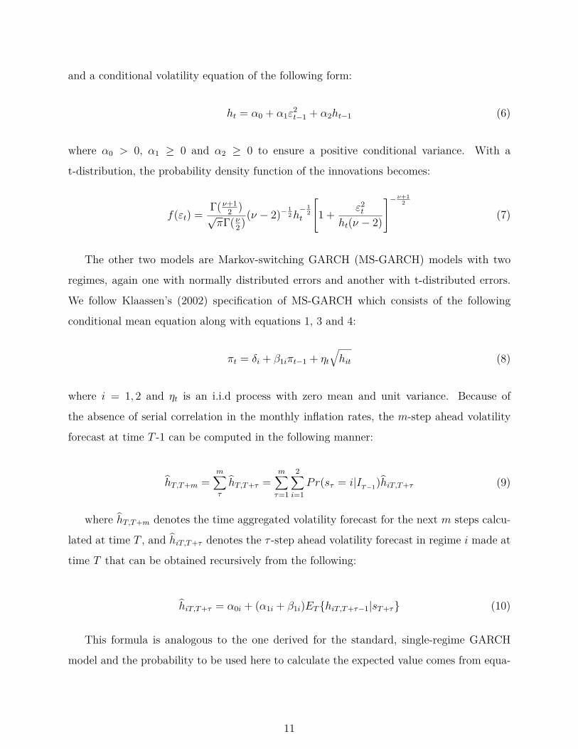
and a conditional volatility equation of the following form:

ht = α0 + α1ε2t−1 + α2ht−1 (6)

where α0 > 0, α1 ≥ 0 and α2 ≥ 0 to ensure a positive conditional variance. With a

t-distribution, the probability density function of the innovations becomes:

f(εt) =Γ(ν+1

2 )√πΓ(ν2 )(ν − 2)− 1

2h− 1

2t

1 + ε2t

ht(ν − 2)

−ν+1

2

(7)

The other two models are Markov-switching GARCH (MS-GARCH) models with two

regimes, again one with normally distributed errors and another with t-distributed errors.

We follow Klaassen’s (2002) specification of MS-GARCH which consists of the following

conditional mean equation along with equations 1, 3 and 4:

πt = δi + β1iπt−1 + ηt√hit (8)

where i = 1, 2 and ηt is an i.i.d process with zero mean and unit variance. Because of

the absence of serial correlation in the monthly inflation rates, the m-step ahead volatility

forecast at time T -1 can be computed in the following manner:

hT,T+m =m∑τ

hT,T+τ =m∑τ=1

2∑i=1

Pr(sτ = i|IT−1)hiT,T+τ (9)

where hT,T+m denotes the time aggregated volatility forecast for the next m steps calcu-

lated at time T , and hiT,T+τ denotes the τ -step ahead volatility forecast in regime i made at

time T that can be obtained recursively from the following:

hiT,T+τ = α0i + (α1i + β1i)ET{hiT,T+τ−1|sT+τ} (10)

This formula is analogous to the one derived for the standard, single-regime GARCH

model and the probability to be used here to calculate the expected value comes from equa-

11

tion 4. Equation 9 suggests that the multi-step ahead volatility forecasts are computed as

a weighted-average of the multi-step-ahead volatility forecasts in each regime estimated ,

where the weights are the prediction probabilities. Using the theory of Markov processes, to

compute the volatility forecasts the filter probability at τ periods ahead Pr (st+τ = i|It) =

pit+τ = M τpit is required where

M =

p11 1− p22

1− p11 p22

(11)

The substantial simplification of the computation of the conditional variance due to the

specification in equation 10 stands as one of the main advantages of Klaassen’s MS-GARCH

model over Gray’s (1996) one. To estimate the Markov regime-switching model parameters,

a quasi-maximum likelihood approach is undertaken with the aid of the ex-ante probability

p1t = Pr (st = 1|It−1) which can be calculated from:

p1t = p11

f(πt−1|st−1 = 1)(1− p1t−1)f(πt−1|st−1 = 1)p1t−1 + f(πt−1|st−1 = 2)(1− p1t−1)

+ (1− p22)

f(πt−1|st−1 = 2)(1− p1t−1)

f(πt−1|st−1 = 1)p1t−1 + f(πt−1|st−1 = 2)(1− p1t−1)

. (12)

Here f (·|st = i) denotes one of the possible conditional distributions from Normal and

Student’s t given that regime i occurs at time t. With the input in equation 11 the log-

likelihood function can be written as:

l =T+w∑

t=−R+w+1log [p1tf (πt|st = 1) + (1− p1t) f (πt|st = 2)] (13)

where w = 0, 1, ...., n. The maximimum likelihood estimates are obtained by maximizing

equation 13 using quasi-Newton algorithm in the Matlab numerical optimization routines.

The estimation is carried out on a moving window of 492 monthly observations.

In this paper, following Marcucci (2005) we evaluate the forecasting performances of

12

competing models with respect to seven statistical loss functions which are listed below:

MSE1 = n−1n∑t=1

(σt+1 − h1/2t+1|t)

2 (14)

MSE2 = n−1n∑t=1

(σt+1 − ht+1|t)2 (15)

QLike = n−1n∑t=1

(loght+1|t + σt+1h−1t+1|t) (16)

R2Log = n−1n∑t=1

[log(σ2t+1h

−1t+1|t)]

2 (17)

MAD1 = n−1n∑t=1|σt+1 − h1/2

t+1|t| (18)

MAD2 = n−1n∑t=1|σ2t+1 − ht+1|t| (19)

HMSE = T−1T∑t=1

(σ2t+1h

−1t+1|t − 1)2 (20)

where σ2 is an estimate of realized volatility and h is volatility forecast from GARCH models.

Equations 14 and 15 are loss functions based on typical mean squared error metrics. The loss

function in equation 16 computes loss implied by a gaussian likelihood and is suggested by

Bollerslev et al. (1994). Equation 17 which is called the Logarithmic Loss Function, penalizes

volatility forecasts asymmetrically in low volatility and high volatility periods (Pagan and

Schwert, 1990). Loss functions in 18 and 19 are particularly useful as they are more robust to

outliers than MSEs. However, these functions do not differentiate between over and under-

predictions while applying the penalty. They are also sensitive to scale transformations.

Bollerslev and Ghysels (1996) have argued that MSE criterion might not be appropriate

in heteroskedastic environment and therefore, suggested heteroskedasticity-adjusted MSE

(HMSE) in equation 20.

In addition to the above statistical loss functions, two non-parametric measures of di-

rectional accuracy are also employed: (i) Success Ratio (SR) and (ii) Directional Accuracy

(DA) test. These measures are generally aimed at computing the number of times a given

model correctly predicts the directions of change of the actual volatility. As Marcucci (2005)

13

has argued, directional accuracy of volatility forecasts bears special significance since they

can be used as inputs to construct various trading strategies such as straddles. SR is defined

as the fraction of the demeaned volatility forecasts that have the same direction of change

as the corresponding demeaned actual volatility. Thus it measures the number of times the

volatility forecast accurately captures the direction of the true volatility process. Formally,

SR can be computed in the following manner:

SR =∑mj=1 I{σt+j ht+j|t+j−1}>0

m(21)

where Ig>0 is an indicator function such that it takes the value of one when the function g

is positive and zero otherwise.

The second test statistic, DA proposed by Pesaran and Timmermann (1992) is computed

as follows:

DA = SR − SRI√Var(SR)− Var(SRI)

(22)

whereSRI = PP + (1− P )(1− P )

Var(SR) = m−1SRI(1− SRI)

Var(SRI ) = m−1(2P − 1)2P (1− P ) +m−1(2P − 1)2P (1− P )

+ 4m−2PP (1− P )(1− P )

(23)

P = m−1m∑j=1

I(σt+j)

P = m−1m∑j=1

I(ht+j|t+j−1)(24)

I(g) =

1 if g > 0

0 otherwise

(25)

In words, P represents the fraction of times that σt+j > 0 and P gives the proportion

14

of demeaned volatility forecasts that are positive. The square of the DA statistic has a

χ2 distribution with one degree of freedom. To compute equations 14 - 22, an estimate

of realized volatilities, σ2 is required. We compute that as squared inflation rates. This

classical approach is used to calculate various financial series’ realized volatilities including

stock market returns.

4 Results

4.1 Single-regime GARCH

Estimation results of standard single-regime GARCH models with both normal and t-

distributions are presented in Table 2. The t-statistics are calculated using asymptotic

standard errors. Across the two models, all of the coefficients in the conditional mean and

variance equations appear to be very similar and are statistically significant. Since the sum-

mation of the estimated ARCH and GARCH parameters, α1 + α2 < 1 for both models,

the assumption of stationarity is satisfied though this violation is common when applying

GARCH models on financial variables for e.g. short-run interest rates. Given these facts, it

can be argued that at least the in-sample performance of standard GARCH models is quite

good. Furthermore, in terms of log-likelihood, GARCH-t performs better than GARCH-n.

This is not entirely unexpected since the histogram and summary statistics provided above

suggested non-normality of inflation rate.

Also, notice that the estimated sum of α1 and α2 is relatively large which is indicative of

high volatility persistence of individual shocks, as argued in the introduction.3 For example,

a shock of 1% to the inflation rate increases the conditional variance at times t+1 to t+5

by respectively 0.203, 0.135, 0.089, 0.059 and 0.039. Whether this high volatility persistence

is spurious can be confirmed by estimating the regime-switching GARCH model. Further,

the excess kurtosis of a t-distribution is given by 6/(ν − 4) which gives a value of 3.97. This

again confirms that the U.S. inflation rate exhibits fat-tailed behavior.3α1 + α2 = 0.87 for normally distributed errors and α1 + α2 = 0.847 for t-distributed errors.

15

Parameters GARCH-N GARCH-t

δ 0.1106*(6.50)

.1084*(6.1425)

β1 0.630*(9.64)

0.629*(9.031)

α0 0.008*(2.86)

0.008*(2.855)

α1 0.203*(4.15)

0.232*(4.412)

α2 0.663*(10.34)

0.639*(9.261)

ν 5.51*(63.53)

Log-Likelihood

14.603 26.318

Table 2: Maximum Likelihood Estimates of Standard GARCH models with normal and t

distributions

4.2 Markov-switching GARCH

Table 3 reports estimates of the Markov-switching GARCHmodels. The second and the third

columns contain the results respectively for the models with normally distributed errors and

t-distributed errors. As characterized by unconditional standard deviations σi, regime 1 has

a slightly higher volatility than regime 2.4 All of the coefficients in the conditional mean

equation of both models appear statistically significant except the intercept term δ2 in the

second regime of MS-GARCH-N. But in the conditional variance equations, four of the total

twelve parameters arise as statistically insignificant, three of which correspond to the MS-

GARCH model with a t distribution. The t-statistics associated with α21 suggest that for4Regime-specific unconditional standard deviations are calculated as σi =

√α0i/(1− α1i − α2i) where

i = 1, 2.

16

both models in regime 1, the GARCH terms are probably not necessary, but in regime 2

they are useful. In fact, MS-GARCH with a t distribution suggests that unlike regime 2,

regime 1 is characterized by a constant variance since both the ARCH coefficient α11 and the

GARCH coefficient α21 are statistically insignificant. With respect to persistence, both MS-

GARCH-N and MS-GARCH-t indicate lower value for regime 1 (higher volatility regime)

than regime 2 (lower volatility regime).

The above results highlight the superior capability of Markov-switching GARCH models

in identifying and distinguishing between different sources of volatility clustering. As Gray

(1996) has argued, volatility clustering has two main sources. The first one is within-regime

persistence and the second one is the persistence of regimes. The implication of regime

persistence is that if the unconditional variance is higher in one regime than the other, then

periods of high volatility tend to cluster together during episodes of high volatility-regime

given that the regimes are persistent. This implies that for US inflation rates, volatility

clustering in regime 1 is caused by the persistence of the high volatility regime and in regime

2 it is caused by both regime persistence and within-regime persistence. After all, the

estimates of regime persistence as given by the transition probabilities p and q in Table 3

are both quite high and statistically significant.

The log-likelihood gives an initial idea of whether regime persistence is an important

source of volatility persistence. For each error distribution, the log-likelihoods correspond-

ing to the regime-switching models are higher than their single-regime counterpart. Hence,

incorporating regimes can be an important mechanism to capture volatility clustering. Also

as expected, estimates of persistence from standard GARCH models fall between the esti-

mates from the high and low volatility regimes produced by the Markov-switching models.

Another interesting result is that the immediate impact of an individual shock seems to be

greater during the higher volatility regime (regime 1) as captured by higher values for the

ARCH term in regime 1, α11 in comparison with the values for the ARCH term in regime

2, α12. This means that for both Markov-switching models in the high volatility regime,

inflationary shocks have a large immediate impact that dies out quickly. But the second

regime’s sensitivities to an individual shock are comparatively low and similar to the ones

17

obtained under standard GARCH models.

The top panel in Figure 3 displays the time series plots of the smoothed, filter and ex

ante probabilities that the inflation rate is in regime 1 at time t as estimated by the MS-

GARCH-N model. MS-GARCH-t model also produces similar plots and therefore, they are

not presented here. According to smoothed probabilities (blue dotted line), there was a

100% probability of the inflation rate being in the high volatility regime until April, 1979.

Eventually, there was a switch to a low volatility regime around mid 1983. These results are

consistent with the finding in the literature that inflation volatility was high in the 1970s but

declined around 1984 during the period of Great Moderation (see Gordon (2007); Blanchard

and Simon (2001); Stock and Watson (2002); Sensier and van Dijk (2004)). This consistency

of result indicates the reliability of our choice of a simple AR(1) conditional mean equation

in the Markov-switching GARCH model.

While the existing studies in the literature only report the break date of 1984, this

paper is the first to present evidence on exactly when the process of structural break in

inflation uncertainty started. According to the smoothed probability plot, the process started

around April 1979 which marginally precedes the nomination of Paul Volcker to serve as the

chairman of the Board of Governors of the Federal Reserve System on July, 1979. Upon

the confirmation of the Senate, Paul Volcker took office on August 6, 1979 and started a

series of contractionary monetary policies including shifting the Fed’s focus to managing the

volume of bank reserves from trying to manage the day-to-day level of the federal funds rate

(Lindsey et al., 2013). Therefore, it can be argued that the process of volatility moderation

closely followed the time frame of the drastic monetary policy changes implemented by the

Fed under Paul Volcker. Nevertheless, to what extent Volcker’s policy changes impacted

inflation volatility or if they affected inflation volatility at all is a separate debate which we

do not seek to settle here.

As a final point before moving on to discuss in-sample goodness-of-fit statistics, both

ex-ante and filter probabilities suggest occurrences of high volatility regimes between (i) late

1987 and late 1990 and (ii) around the onset of the 2007 recession. However, once information

18

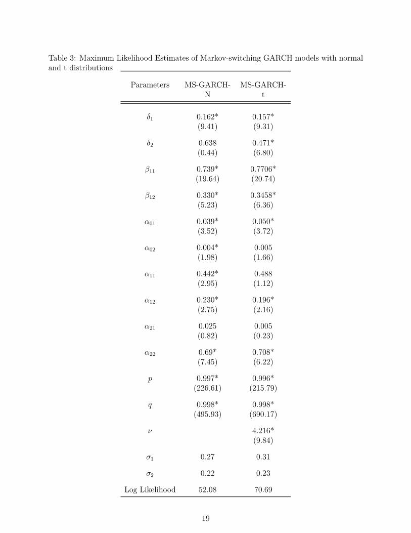
Table 3: Maximum Likelihood Estimates of Markov-switching GARCH models with normaland t distributions

Parameters MS-GARCH-N

MS-GARCH-t

δ1 0.162*(9.41)

0.157*(9.31)

δ2 0.638(0.44)

0.471*(6.80)

β11 0.739*(19.64)

0.7706*(20.74)

β12 0.330*(5.23)

0.3458*(6.36)

α01 0.039*(3.52)

0.050*(3.72)

α02 0.004*(1.98)

0.005(1.66)

α11 0.442*(2.95)

0.488(1.12)

α12 0.230*(2.75)

0.196*(2.16)

α21 0.025(0.82)

0.005(0.23)

α22 0.69*(7.45)

0.708*(6.22)

p 0.997*(226.61)

0.996*(215.79)

q 0.998*(495.93)

0.998*(690.17)

ν 4.216*(9.84)

σ1 0.27 0.31

σ2 0.22 0.23

Log Likelihood 52.08 70.69

19

Figure 3: The top panel contains a time series plot of the smoothed, filter and ex anteprobabilities that the inflation rate is in regime 1 at time t according to the MS-GARCH-Nmodel. The bottom panel displays the same probabilities for regime 2.

from the whole sample is taken into account by smoothed probabilities, it becomes clear that

neither of these periods actually correspond to high volatility regimes. Another alternative

explanation based on ex-ante probabilities with respect to the period around the onset of

the 2007 recession is possible. (Klaassen, 2002) has argued that some large shocks are are

not persistent at all and have a rather “pressure relieving” effect. Since the within-regime

persistence estimated in this paper for the high volatility regime is low, the effect of the

shock to inflation volatility dies out quickly before switching to the low volatility regime.

In that sense, the shock to the inflation volatility before the recession of 2007 imparted a

“pressure relieving” effect. This is depicted in Figure 4 as a spike in the conditional volatility

around the time of the recession in 2007.

20

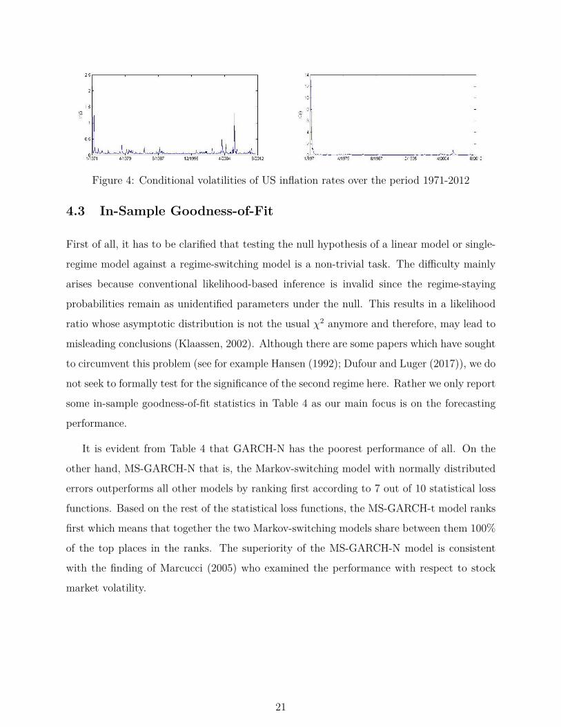
Figure 4: Conditional volatilities of US inflation rates over the period 1971-2012

4.3 In-Sample Goodness-of-Fit

First of all, it has to be clarified that testing the null hypothesis of a linear model or single-

regime model against a regime-switching model is a non-trivial task. The difficulty mainly

arises because conventional likelihood-based inference is invalid since the regime-staying

probabilities remain as unidentified parameters under the null. This results in a likelihood

ratio whose asymptotic distribution is not the usual χ2 anymore and therefore, may lead to

misleading conclusions (Klaassen, 2002). Although there are some papers which have sought

to circumvent this problem (see for example Hansen (1992); Dufour and Luger (2017)), we do

not seek to formally test for the significance of the second regime here. Rather we only report

some in-sample goodness-of-fit statistics in Table 4 as our main focus is on the forecasting

performance.

It is evident from Table 4 that GARCH-N has the poorest performance of all. On the

other hand, MS-GARCH-N that is, the Markov-switching model with normally distributed

errors outperforms all other models by ranking first according to 7 out of 10 statistical loss

functions. Based on the rest of the statistical loss functions, the MS-GARCH-t model ranks

first which means that together the two Markov-switching models share between them 100%

of the top places in the ranks. The superiority of the MS-GARCH-N model is consistent

with the finding of Marcucci (2005) who examined the performance with respect to stock

market volatility.

21

Table 4: In-sample goodness-of-fit statistics

Model NumPar AIC Rank BIC Rank LogL Rank MSE1 Rank MSE2 Rank QLike Rank R2Log Rank MAD2 Rank MAD1 Rank HMSE Rank

GARCH-N 5 -0.03 4.00 0.02 4.00 11.23 4.00 0.06 3.00 0.12 3.00 -1.34 3.00 5.79 3.00 0.12 3.00 0.16 3.00 6.81 3.00

GARCH-t 6 -0.09 3.00 -0.04 3.00 28.71 3.00 0.06 2.00 0.12 2.00 -1.37 2.00 5.81 4.00 0.12 2.00 0.16 2.00 6.38 2.00

MS-GARCH-N 12 -0.16 2.00 -0.06 2.00 52.04 2.00 0.05 1.00 0.08 1.00 -1.43 1.00 5.37 1.00 0.11 1.00 0.15 1.00 6.12 1.00

MS-GARCH-t 13 -0.23 1.00 -0.12 1.00 70.69 1.00 0.07 4.00 0.23 4.00 -1.23 4.00 5.70 2.00 0.13 4.00 0.17 4.00 9.20 4.00

Note: NumPar is the number of parameters estimated in each model, AIC is Akaike Information Criterion calculated as−2log(L)/T+

2k/T where k is the number of parameters and T is the total number of observations. BIC is the Bayesian Information Criterion or

Schwarz Criterion calculated as −2log(L)/T + (k/T ). The rest of the statistical loss functions MSE1, MSE2, QLike, R2Log, MAD1,

MAD2, and HMSE are defined in Section 3.

22

4.4 Out-of-Sample Forecasting Performance

One particular caveat about the previous section’s results is that highly parameterized models

tend to produce good in-sample fits. Therefore, one needs to be careful about the appar-

ent superiority of Markov-switching models in terms of their in-sample performance since

they are inherently highly parameterized. In contrast, out-of-sample tests are capable of

controlling either possible over-fitting or over-parameterization problems (Marcucci, 2005).

Therefore, in this section we examine and compare with each other the out-of-sample per-

formances of the previous four variants of GARCH models in forecasting inflation volatility.

Out-of-sample volatility forecasting performance is important also because of its relevance

to researchers and practitioners.

Tables 5 to 10 report 1 to 12-month ahead inflation uncertainty forecasting performances

in terms of the seven statistical loss functions defined in Section 3. They also report estimates

for Success Ratio (SR) and Directional Accuracy (DA) test statistic. It is clear that MS-

GARCH-N clearly outperforms all other models in forecasting inflation uncertainty 1 to

5-month ahead. For the same forecasting horizon, MS-GARCH-t ranks second best while

GARCH-N fares worst. These rankings are consistent with in-sample performances found

in Section 4.2. However, note that unlike for other models the DA test statistic for MS-

GARCH-N is not statistically significant.5 Nevertheless, MS-GARCH-N has the highest SR

value for each forecast horizon from 1 to 5 months.

For forecast horizons of 6 and 7 months, both Markov-switching GARCH models have

comparable performances. Standard GARCH models still perform worse than their regime-

switching counterparts. From 8-month ahead horizon onward, MS-GARCH-t starts exceed-

ing all other models in forecasting performance. In fact, for the 12-month ahead volatility

forecasts, MS-GARCH-t ranks 1 in 6 out of 7 statistical loss functions. Also notice that be-

yond 5-month forecast horizon, MS-GARCH-N has a statistically significant DA test statis-

tic. However, its performance clearly declines from 10-month forecast horizon onward when5The square of DA test statistics for MS-GARCH-N are less than the 5% significance level χ2 critical value

3.84. Therefore, we fail to reject the null hypothesis that forecasted conditional volatility cannot predictrealized volatility.

23

even standard GARCH-t performs better than MS-GARCH-N. In a nutshell, for short-term

forecast horizon spanning 1 to 5-months, Markov-switching GARCH model with normally

distributed errors (MS-GARCH-N) performs better than the other three GARCH models.

But for longer horizons, MS-GARCH-t performs better in terms of out-of-sample forecasting

evaluation.

5 Conclusion

Volatility of inflation rate or inflation uncertainty is as important a variable as the level of

inflation rate. It has serious welfare loss implications for risk averse economic agents even

if all the prices in the economy are fully flexible. Therefore, being able to forecast inflation

uncertainty as accurately as possible is of paramount importance. Coupled with that is the

fact that a casual “eyeballing” of the data on US inflation rates from 1971 to present suggests

that its volatility might have undergone regime changes multiple times. Existing studies in

the literature also confirm at least one structural break in 1984. Therefore, it might be

appropriate to forecast inflation uncertainty using Markov-switching GARCH models which

are capable of handling regime changes unlike standard GARCH models.

Modeling inflation uncertainty using regime-switching GARCH models also provides the

opportunity to evaluate the forecasting performance of these models relative to standard

ones. In this paper, we seize that opportunity to augment the existing evidences which

already support regime-switching GARCH models’ superior shorter horizon forecasting per-

formance. However, those evidences are based on only stock market and exchange rate data.

Following Marcucci (2005), this paper employs a broad set of statistical loss functions to

evaluate the relative performances of Markov-switching GARCH models in forecasting US

inflation uncertainty.

One of the first major findings of this paper is that a Markov-regime switching GARCH

model consisting of a simple AR(1) conditional mean equation does remarkably well in iden-

tifying US inflation uncertainty’s structural shift in the year 1984. This result is consistent

24

with the general agreement in the literature on the break date. In addition, this paper has

identified April, 1979 as the time when the regime switching process might have started

before culminating in a complete switch in 1984. The whole switching process mirrors the

time line which follows a specific period that starts from the nomination of Paul Volcker as

the new chairman of the Federal Reserve System to his implementation of various drastic

monetary policy initiatives until 1984.

Another important result of this paper is that in the high volatility regime, shock per-

sistence is lower compared to the low volatility regime. But the immediate impact of an

individual inflationary shock is higher in the high volatility regime. New evidences are pre-

sented which show that the main source of volatility clustering in the high volatility regime

is caused by the persistence of the regime itself. Finally, a comparison of the forecasting

performances of the four different GARCH models indicates that for a forecasting horizon of

1 to 5 months, a Markov regime-switching GARCH model with normally distributed errors

(MS-GARCH-N) outperforms all other three models. However, for longer forecasting horizon

such as 8 to 12 months, a Markov regime-switching GARCH model with t distributed errors

(MS-GARCH-t) performs the best. For the same longer horizon, MS-GARCH-N performs

poorly even compared to a standard GARCH model with t distributed errors.

The results and analyses of this paper can be extended in the future to explore the

relationship between inflation and inflation uncertainty within a regime-switching framework.

Also, forecasting exercises similar to the ones in this paper can also be carried out for other

countries’ inflation rates. It will be interesting to further evaluate the relative performances

of Markov regime-switching GARCH models in the contexts of different economic settings.

25

Table 5: Out-of-sample evaluation of one and two-month ahead volatility forecasts1-month ahead volatility forecasts

Model MSE1 Rank MSE2 Rank QLike Rank R2Log Rank MAD2 Rank MAD1 Rank HMSE Rank SR DA

GARCH-N 0.0048 4 0.0088 4 -2.7139 3 1.5208 2 0.1453 4 0.0594 4 1.2004 2 0.36 -3.9767

GARCH-t 0.003 3 0.0088 3 -2.9989 4 0.0026 1 0.1372 3 0.057 3 1.4516 3 0.38 -3.8858

MS-GARCH-N 0.0189 1 0.0042 1 -2.1548 2 5.2561 3 0.1116 1 0.0467 1 0.7784 1 0.51 -1.9727

MS-GARCH-t 0.0212 2 0.0047 2 -1.9906 1 5.6603 4 0.1208 2 0.0495 2 1.7038 4 0.44 -3.7334

2-month ahead volatility forecasts

Model MSE1 Rank MSE2 Rank QLike Rank R2Log Rank MAD2 Rank MAD1 Rank HMSE Rank SR DA

GARCH-N 0.0048 4 0.0088 4 -2.7139 3 1.5208 2 0.1453 4 0.0594 4 1.2004 2 0.36 -3.9767

GARCH-t 0.003 3 0.0088 3 -2.9989 4 0.0026 1 0.1372 3 0.057 3 1.4516 3 0.38 -3.8858

MS-GARCH-N 0.0189 1 0.0042 1 -2.1548 2 5.2561 3 0.1116 1 0.0467 1 0.7784 1 0.51 -1.9727

MS-GARCH-t 0.0212 2 0.0047 2 -1.9906 1 5.6603 4 0.1208 2 0.0495 2 1.7038 4 0.44 -3.7334

26

Table 6: Out-of-sample evaluation of three and four-month ahead volatility forecasts3-month ahead volatility forecasts

Model MSE1 Rank MSE2 Rank QLike Rank R2Log Rank MAD2 Rank MAD1 Rank HMSE Rank SR DA

GARCH-N 0.0198 4 0.0409 4 -4.3265 4 0.5748 2 0.2155 4 0.1399 4 344.0068 4 0.41 -2.5931

GARCH-t 0.0157 3 0.0399 3 0.4847 1 0.4252 1 0.2064 3 0.1358 3 75.8866 3 0.44 -2.4503

MS-GARCH-N 0.0334 1 0.021 1 -0.9934 3 1.5323 3 0.1456 1 0.1107 1 0.4615 1 0.51 -1.4759

MS-GARCH-t 0.0366 2 0.0222 2 -0.9135 2 1.675 4 0.153 2 0.113 2 0.7898 2 0.49 -2.172

4-month ahead volatility forecasts

Model MSE1 Rank MSE2 Rank QLike Rank R2Log Rank MAD2 Rank MAD1 Rank HMSE Rank SR DA

GARCH-N 0.0401 4 0.0706 4 -0.9952 3 -0.0826 1 0.2382 4 0.1849 4 2.1482 4 0.38 -2.7801

GARCH-t 0.0378 3 0.0692 3 -1.0669 4 -0.2367 2 0.2309 3 0.1808 3 1.8226 3 0.41 -2.627

MS-GARCH-N 0.0442 1 0.0344 1 -0.6642 2 1.3966 3 0.1661 1 0.1453 1 0.4674 1 0.49 -1.6718

MS-GARCH-t 0.0468 2 0.0355 2 -0.5998 1 1.4809 4 0.1806 2 0.1537 2 0.7232 2 0.41 -3.1542

27

Table 7: Out-of-sample evaluation of five and six-month ahead volatility forecasts5-month ahead volatility forecasts

Model MSE1 Rank MSE2 Rank QLike Rank R2Log Rank MAD2 Rank MAD1 Rank HMSE Rank SR DA

GARCH-N 0.062 4 0.0991 4 -1.1493 3 0.0616 1 0.2661 4 0.232 4 6.9225 3 0.33 -3.1563

GARCH-t 0.0602 3 0.0971 3 -1.3805 4 0.0097 2 0.2593 3 0.228 3 10.4287 4 0.36 -2.9824

MS-GARCH-N 0.055 1 0.0509 2 -0.3972 2 1.3432 3 0.1818 1 0.1738 1 0.5602 1 0.49 -1.2888

MS-GARCH-t 0.0559 2 0.05 1 -0.36 1 1.3832 4 0.1988 2 0.1867 2 0.6854 2 0.41 -2.6436

6-month ahead volatility forecasts

Model MSE1 Rank MSE2 Rank QLike Rank R2Log Rank MAD2 Rank MAD1 Rank HMSE Rank SR DA

GARCH-N 0.0756 4 0.1227 4 -0.5359 3 0.2616 2 0.2823 4 0.2706 4 3.3074 4 0.38 -2.4236

GARCH-t 0.0745 3 0.12 3 -0.6228 4 0.1868 1 0.2744 3 0.2644 3 3.0855 3 0.41 -2.2368

MS-GARCH-N 0.0657 2 0.0702 2 -0.1885 2 1.3152 3 0.199 1 0.2043 1 0.5717 1 0.44 -2.0503

MS-GARCH-t 0.0647 1 0.0667 1 -0.1724 1 1.321 4 0.2165 2 0.2209 2 0.6123 2 0.36 -3.4247

28

Table 8: Out-of-sample evaluation of seven and eight-month ahead volatility forecasts7-month ahead volatility forecasts

Model MSE1 Rank MSE2 Rank QLike Rank R2Log Rank MAD2 Rank MAD1 Rank HMSE Rank SR DA

GARCH-N 0.0858 4 0.1345 4 -0.6945 3 0.2278 1 0.2851 4 0.2874 4 5.0744 3 0.36 -2.6304

GARCH-t 0.0859 3 0.1313 3 -0.8356 4 0.2232 2 0.278 3 0.2813 3 7.102 4 0.38 -2.4333

MS-GARCH-N 0.0781 2 0.0974 2 -0.0201 2 1.3184 4 0.221 1 0.2453 1 0.5687 1 0.41 -2.2368

MS-GARCH-t 0.0742 1 0.089 1 -0.0175 1 1.2886 3 0.2302 2 0.2532 2 0.5944 2 0.33 -3.5687

8-month ahead volatility forecasts

Model MSE1 Rank MSE2 Rank QLike Rank R2Log Rank MAD2 Rank MAD1 Rank HMSE Rank SR DA

GARCH-N 0.0936 4 0.1446 4 -1.5086 3 0.3767 1 0.2862 4 0.3043 4 41.4512 3 0.38 -2.133

GARCH-t 0.0934 3 0.1412 3 36.3074 4 1.9969 4 0.2802 3 0.2997 3 37865.0154 4 0.41 -1.913

MS-GARCH-N 0.0898 2 0.1295 2 0.1192 2 1.2825 3 0.246 2 0.2952 2 0.5445 1 0.38 -2.4236

MS-GARCH-t 0.0822 1 0.1131 1 0.1105 1 1.2208 2 0.2416 1 0.2842 1 0.5613 2 0.31 -3.719

29

Table 9: Out-of-sample evaluation of nine and ten-month ahead volatility forecasts9-month ahead volatility forecasts

Model MSE1 Rank MSE2 Rank QLike Rank R2Log Rank MAD2 Rank MAD1 Rank HMSE Rank SR DA

GARCH-N 0.0942 4 0.1558 3 0.438 4 0.6243 2 0.2902 4 0.3268 3 13.7268 4 0.36 -2.3527

GARCH-t 0.0932 3 0.1528 2 0.1126 3 0.5168 1 0.2854 3 0.3243 2 5.0627 3 0.38 -2.122

MS-GARCH-N 0.1019 2 0.1648 4 0.239 2 1.2903 4 0.2716 2 0.3487 4 0.5054 1 0.36 -2.612

MS-GARCH-t 0.0906 1 0.1386 1 0.2227 1 1.2054 3 0.2533 1 0.3154 1 0.5239 2 0.28 -3.8759

10-month ahead volatility forecasts

Model MSE1 Rank MSE2 Rank QLike Rank R2Log Rank MAD2 Rank MAD1 Rank HMSE Rank SR DA

GARCH-N 0.1064 3 0.1843 3 0.115 2 0.5126 1 0.2971 4 0.3571 3 4.9909 4 0.36 -2.3527

GARCH-t 0.1077 4 0.1828 2 -0.0347 1 0.5078 2 0.2943 3 0.3561 2 4.3118 3 0.41 -1.6576

MS-GARCH-N 0.1127 2 0.2041 4 0.3437 4 1.2571 4 0.2886 2 0.3941 4 0.4921 1 0.33 -2.8294

MS-GARCH-t 0.0975 1 0.1654 1 0.3198 3 1.1527 3 0.2617 1 0.3445 1 0.5012 2 0.28 -3.8759

30

Table 10: Out-of-sample evaluation of eleven and twelve-month ahead volatility forecasts11-month ahead volatility forecasts

Model MSE1 Rank MSE2 Rank QLike Rank R2Log Rank MAD2 Rank MAD1 Rank HMSE Rank SR DA

GARCH-N 0.1136 2 0.2021 2 -0.1639 1 0.5188 1 0.2969 4 0.3738 2 7.9816 3 0.41 -1.8895

GARCH-t 0.1171 3 0.2033 3 -0.6314 4 0.6516 2 0.2955 2 0.3744 3 22.4232 4 0.41 -1.6576

MS-GARCH-N 0.1214 4 0.2446 4 0.4396 3 1.1945 4 0.296 3 0.4278 4 0.4719 2 0.33 -2.8294

MS-GARCH-t 0.1019 1 0.1909 1 0.4087 2 1.0713 3 0.2607 1 0.3615 1 0.4696 1 0.28 -3.8759

12-month ahead volatility forecasts

Model MSE1 Rank MSE2 Rank QLike Rank R2Log Rank MAD2 Rank MAD1 Rank HMSE Rank SR DA

GARCH-N 0.1192 3 0.2337 2 2.8951 4 1.2391 4 0.3038 3 0.4095 2 185.8821 4 0.33 -3.1633

GARCH-t 0.1184 2 0.2372 3 0.9242 3 0.8923 1 0.3012 2 0.4132 3 10.5512 3 0.31 -3.3477

MS-GARCH-N 0.133 4 0.2972 4 0.569 2 1.1636 3 0.3126 4 0.4771 4 0.5014 2 0.23 -4.6233

MS-GARCH-t 0.1086 1 0.225 1 0.5292 1 1.0204 2 0.2709 1 0.3968 1 0.4775 1 0.18 -5.8629

31

References

Andersen, T. G. and Bollerslev, T. (1998). Answering the Skeptics: Yes, Standard Volatility

Models do Provide Accurate Forecasts. International Economic Review, 39(4):885–905.

Barnea, A., Dotan, A., and Lakonishok, J. (1979). The Effect of Price Level Uncertainty

on the Determination of Nominal Interest Rates: Some Empirical Evidence. Southern

Economic Journal, 46(2):609–614.

Blanchard, O. and Simon, J. (2001). The Long and Large Decline in U.S. Output Volatility.

Bollerslev, T. (1986). Generalized autoregressive conditional heteroskedasticity. Journal of

Econometrics, 31(3):307–327.

Bollerslev, T., Engle, R. F., and Nelson, D. B. (1994). ARCH Models. In Handbook of

Econometrics, volume 4, pages 2959–3038.

Bollerslev, T. and Ghysels, E. (1996). Periodic Autoregressive Conditional Heteroscedastic-

ity. Journal of Business & Economic Statistics, 14(2):139–151.

BREDIN, D. O. N. and FOUNTAS, S. (2005). MACROECONOMIC UNCERTAINTY

ANDMACROECONOMIC PERFORMANCE: ARE THEY RELATED? The Manchester

School, 73:58–76.

Cai, J. (1994). A Markov Model of Switching-Regime ARCH. Journal of Business & Eco-

nomic Statistics, 12(3):309–316.

Caporale, G. M., Onorante, L., and Paesani, P. (2010). Inflation and inflation uncertainty

in the euro area.

Chang, K.-L. and He, C.-W. (2010). DOES THE MAGNITUDE OF THE EFFECT OF

INFLATION UNCERTAINTY ON OUTPUT GROWTH DEPEND ON THE LEVEL OF

INFLATION? The Manchester School, 78(2):126–148.

Dotsey, M. and Sarte, P. D. (2000). Inflation uncertainty and growth in a cash-in-advance

economy. Journal of Monetary Economics, 45(3):631–655.

32

Dueker, M. (1997). Markov Switching in GARCH Processes and Mean- Reverting Stock-

Market Volatility. Journal of business & Economics Statistics, 15(1):26–34.

Dufour, J.-M. and Luger, R. (2017). Identification-robust moment-based tests for Markov

switching in autoregressive models. Econometric Reviews, 36(6-9):713–727.

Engle, R. F. . (1982). Autoregressive Conditional Heteroscedasticity with Estimates of the

Variance of United Kingdom Inflation Author ( s ): Robert F . Engle Published by : The

Econometric Society Stable URL : http://www.jstor.org/stable/1912773 REFERENCES

Linked references ar. Econometrica, 50(4):987–1007.

Engle, R. F. (1983). Estimates of the Variance of U . S . Inflation Based upon the ARCH

Model Author ( s ): Robert F . Engle Source : Journal of Money , Credit and Banking ,

Vol . 15 , No . 3 ( Aug ., 1983 ), pp . 286-301 Published by : Blackwell Publishing Stable

URL : http:. Journal of Money , Credit and Banking, 15(3):286–301.

Evans, M. (1991). Discovering the Link Between Inflation Rates and Inflation Uncertainty.

Journal of Money, Credit and Banking, 23(2):169–184.

Fischer, S. (1981). Towards an understanding of the costs of inflation: II. Carnegie-Rochester

Conference Series on Public Policy, 15:5–41.

Fischer, S. and Modigliani, F. (1978). Towards an understanding of the real effects and costs

of inflation. Weltwirtschaftliches Archiv, 114(4):810–833.

Fountas, S., Karanasos, M., and Kim, J. (2006). Inflation Uncertainty, Output Growth Un-

certainty and Macroeconomic Performance. Oxford Bulletin of Economics and Statistics,

68(3):319–343.

Friedman, M. (1977). Nobel Lecture: Inflation and Unemployment. Journal of Political

Economy, 85(3):451–472.

Giordani, P. and Söderlind, P. (2003). Inflation forecast uncertainty. European Economic

Review, 47(6):1037–1059.

33

Gordon, R. J. (2007). Phillips Curve specification and the decline in US output and inflation

volatility. In Symposium on the Phillips Curve and the Natural Rate of Unemployment,

Institut fur Weltwirtschaft, Kiel Germany, June, volume 4.

Gray, S. F. (1996). Modeling the conditional distribution of interest rates as a regime-

switching process. Journal of Financial Economics, 42(1):27–62.

Grier, K. B., Henry, Ó. T., Olekalns, N., and Shields, K. (2004). The asymmetric effects of

uncertainty on inflation and output growth. Journal of Applied Econometrics, 19(5):551–

565.

Grier, K. B. and Perry, M. J. (1998). On inflation and inflation uncertainty in the G7

countries. Journal of International Money and Finance, 17(4):671–689.

Hamilton, J. D. (1988). Rational-expectations econometric analysis of changes in regime.

Journal of Economic Dynamics and Control, 12(2-3):385–423.

Hamilton, J. D. (1989). A New Approach to the Economic Analysis of Nonstationary Time

Series and the Business Cycle. Econometrica, 57(2):357–384.

Hamilton, J. D. and Susmel, R. (1994). Autoregressive conditional heteroskedasticity and

changes in regime. Journal of Econometrics, 64(1):307–333.

Hansen, B. E. (1992). The likelihood ratio test under nonstandard conditions: Testing the

markov switching model of gnp. Journal of Applied Econometrics, 7(S1):S61–S82.

Holland, A. S. (1995). Inflation and Uncertainty: Tests for Temporal Ordering. Journal of

Money, Credit and Banking, 27(3):827–837.

Kim, C.-J. (1994). Dynamic linear models with Markov-switching. Journal of Econometrics,

60(1-2):1–22.

Klaassen, F. (2002). EMPIRICAL Improving GARCH volatility forecasts with regime-

switching GARCH. Empirical Economics, (27):363–394.

34

Kontonikas, A. (2004). Inflation and inflation uncertainty in the United Kingdom, evidence

from GARCH modelling. Economic Modelling, 21(3):525–543.

Lahiri, K. and Sheng, X. (2010). Measuring forecast uncertainty by disagreement: The

missing link. Journal of Applied Econometrics, 25(4):514–538.

Lamoureux, C. G. and Lastrapes, W. D. (1990). Persistence in Variance, Structural Change,

and the GARCH Model. Journal of Business & Economic Statistics, 8(2):225–234.

Lindsey, D. E., Orphanides, A., and Rasche, R. H. (2013). The Reform of October 1979:

How It Happened and Why. Federal Reserve Bank of St. Louis Review, pages 487–542.

Marcucci, J. (2005). Forecasting Stock Market Volatility with Regime-Switching GARCH

models. Studies in Nonlinear Dynamics & Econometrics, 9(4).

Melvin, M. (1982). Expected Inflation, Taxation, and Interest Rates: The Delusion of Fiscal

Illusion. The American Economic Review, 72(4):841–845.

Pagan, A. R. and Schwert, G. (1990). Alternative models for conditional stock volatility.

Journal of Econometrics, 45(1-2):267–290.

Pesaran, M. H. and Timmermann, A. (1992). A Simple Nonparametric Test of Predictive

Performance. Journal of Business & Economic Statistics, 10(4):461–465.

Pindyck, R. (1991). No Title. Journal of Economic Literature, 29:1110–1148.

Sensier, M. and van Dijk, D. (2004). Testing for Volatility Changes in U.S. Macroeconomic

Time Series. The Review of Economics and Statistics, 86(3):833–839.

Stock, J. H. and Watson, M. W. (2002). Has the Business Cycle Changed and Why? NBER

Macroeconomics Annual, 17:159–218.

35