Embed Size (px)
Citation preview
MPRAMunich Personal RePEc Archive
Financial Repression and HousingInvestment: An Analysis of the KoreanChonsei
Jinwon Kim
1. August 2012
Online at http://mpra.ub.uni-muenchen.de/47586/MPRA Paper No. 47586, posted 15. June 2013 09:27 UTC

Financial Repression and Housing Investment: AnAnalysis of the Korean Chonsei
Jinwon Kim∗
First Version: August 2012Current Version: May 2013
Abstract
South Korea has a unique kind of rental contract, called chonsei. The tenant pays an upfront
deposit, typically from 40% to 70% of the property value, to the landlord, and the landlord
repays the deposit to the tenant upon contract termination. The tenant is not required
to make any periodic monthly rental payments. The main goal of this paper is to show
why such a unique rental contract exists and has been popular in Korea. The model shows
that chonsei is an ingenious market response in the era of “financial repression” in Korea
(Renaud (1989)), allowing landlords to accumulate sufficient funds for housing investment
without major reliance on a mortgage. The model also shows that the tenant, who suffers
from insufficient mortgage borrowings, can access cheaper rental housing via chonsei than
when only monthly rental housing is available. The model predicts that the chonsei system
should fade out when arbitrage gains from housing investment disappear. An implication of
the model is that the chonsei renter may save while the landlord and the owner-occupier put
all their assets into housing and thus have no financial savings. This hypothesis is empirically
tested and confirmed.
Keywords : Chonsei, Korean housing market, Financial repression, Household saving,
Tenure choice
JEL Classification Numbers : R2, G2, D1
∗Technical University of Denmark, 2800 Kgs. Lyngby, Denmark. Email: [email protected]. I amdeeply indebted to my adviser Jan Brueckner for his guidance, encouragement, and support. I am alsograteful to Volodymyr Bilotkach, David Brownstone, Vernon Henderson, Priya Ranjan, Kenneth Small, andJoseph Tracy for helpful comments. I also wish to thank Kyung-Hwan Kim, Edith Madsen, Ismir Mulalic,Albert Saiz, and seminar participants at the 2012 Urban Economics Association Meetings for valuablediscussions.
1

1 Introduction
South Korea (Korea hereafter) has a unique way of renting a house, called chonsei. The
tenant pays an upfront lump-sum deposit, which is typically from 40% to 70% of the property
value, to the landlord for the use of the property. The landlord repays the nominal value of
the deposit to the tenant upon contract termination. There is no additional requirement for
the tenant such as periodic rental payments. So, the chonsei deposit, which is held during
the contract period and repaid by the landlord, is the substitute for such payments.1
Chonsei became increasingly popular in Korea over the past few decades as the country
experienced rapid economic development and urbanization.2 Chonsei is still a popular tenure
choice in Korea. As of 2010, about 22% of national households and 33% of households in
Seoul live in chonsei rental housing while 54% of the national households reside in owner-
occupied housing. Chonsei accounts for about 50% of the rental housing market. Moreover,
including the mixed form of chonsei and monthly rent, the portion of chonsei-type contract is
92% in the rental housing market. Only 8% of rental houses are pure monthly rental units.3
Many authors point out that financial market imperfection during the period of eco-
nomic development has led to the popularity of the chonsei rental system in Korea (Renaud
(1989), Kim (1990), Son (1997)). Government policies aimed at boosting the national econ-
omy helped financial institutions supply cheap credit to the industrial sector. Due to the
successful economic development plans, Korea experienced rapid economic growth and ur-
banization between 1960 and 1990. The Korean housing sector, however, had to undergo
1Chonsei-type rental contracts are not entirely unique to Korea. The antichresis lease, which appears inmany civil law countries, also requires a lump sum tenant payment that is to be returned in full at the endof the lease. Chonsei can actually be regarded as a version of the antichresis lease contract. The countrieswhere the antichresis lease contract is used include Argentina, Bolivia, Egypt, France, and Spain. Navarroand Turnbull (2010) explore the antichresis from the Bolivian experience, with their emphases being tenantliquidity risk and owner input moral hazard.
2It is known that the kind of chonsei rental contract existed hundreds years ago in Korea, but it is unclearwhen chonsei was first used.
3The mixed form of chonsei and monthly rent, which we call “mixed chonsei,” requires that the tenantpay a mixture of an upfront deposit and monthly rents. The tenant does not pay the full chonsei deposit, butinstead pays monthly rents to fill the gap. The source of the statistics is Statistics Korea (http://kostat.go.kr).
2

“financial repression” during the same period (Renaud (1989)).4 Under financial repression,
the real returns on financial savings were reduced by interest rate ceilings due to the gov-
ernment policies favoring the industrial sector. On the other hand, household savings via
housing ownership were not disadvantaged by the government policies. Rather, investments
in housing were encouraged as the rapid urbanization in major cities caused the demand
for housing to rise sharply. Meanwhile, housing was in short supply in Korean cities, partly
due to strong government land-use controls, and given high demand, people expected high
capital gains from house ownership (Kim (1990)). Thus, due to financial repression and the
housing shortage problem in major cities, housing has been regarded as a superior invest-
ment compared to financial savings, with house price rising faster than real income or any
other price variables during the period of economic development (Son (1997)). Moreover,
the rate of house price appreciation was much greater than real interest rates during this
period (Mills and Song (1977)).5
Although the Korean households were inclined to own houses, they were constrained in
their ability to borrow to invest in owner-occupied housing. While most financial institutions
were geared to supply funds to the industrial sector, Korean households could not access
sufficient finances. Especially, mortgage borrowing was almost unavailable to consumers
until recently. Only about 10% of homebuyers received mortgage loans, and the loan-to-
value (LTV) ratio was less than 30% between 1970 and 1985 (Kim (1990), Gyourko and
Han (1989)). Under such a poor housing finance system, Korean consumers with low initial
wealth could not purchase a house, despite high expected capital gains from house ownership.
In addition, strong government regulations in the housing and the rental housing markets
have caused a lack of organized rental entities. Government policies have been biased to-
ward the supply of new owner-occupied housing units, instead of supplying sufficient rental
housing units (Son (1997)). For example, the government’s credit rationing policies required
4“Financial repression” is a kind of deliberate government policy designed to channel funds to the gov-ernment or the industrial sector and thus obtain explicit or indirect control over interest rates.
5The detailed data on house prices has become available since 1987, much later than the chonsei systemgained its original popularity.
3

that rental housing developers operate with a high capital-to-debt ratio (Ambrose and Kim
(2003)). As a result, sufficient rental housing units, which would fill the rapidly increasing
demand for housing in urbanizing areas, were not supplied by institutionalized entities such
as rental companies and the government. Instead, most rental houses in Korea have been
supplied by private households.
The chonsei system was an ingenious response by the housing sector to the conditions
of the Korean housing market described above. A chonsei deposit can satisfy the landlord’s
financial needs to invest in housing. Chonsei is also beneficial to the tenant because the
tenant can access cheaper rental housing via a chonsei contract than via a monthly rental
contract, which will be explicit in the model below.
Although there is a considerable consensus about the reasons for the existence and the
popularity of the chonsei system in Korea, there have been no formal models that explicitly
capture the widely recognized sources of the chonsei system. Ambrose and Kim (2003)
study the default option in chonsei, and Kim and Shin (2011) focus on the role of financial
intermediation in the chonsei system. But, these studies look at different aspects of chonsei,
without directly focusing on its main properties. In our model, we explicitly analyze both the
landlord’s and the tenant’s problems, viewing housing as an investment, while incorporating
the housing market conditions in Korea. Under our framework, we can show how chonsei
emerges in equilibrium and provide better insights about the chonsei rental contract.
Specifically, in our model, a private landlord decides how much housing to buy and
what portion of this amount to rent out to tenants, with the balance consumed as an
owner-occupier. Owner-occupied housing is viewed as an investment, as in Henderson and
Ioannides (1983) and Brueckner (1997). The consumer is faced with several borrowing con-
straints, reflecting the financial market imperfection in Korea. For instance, the consumer
cannot borrow against future incomes. The consumer can instead rely on mortgage borrow-
ing by offering houses as collateral. But, there is a loan-to-value (LTV) constraint, which
requires that the mortgage borrowing must be significantly smaller than the property value.
4
Landlords, seeking a profitable investment return, combine their initial wealth with limited
mortgage funds to buy housing. Lacking adequate funds to supplement with mortgage bor-
rowing, consumers with low initial wealth will be unable to buy a house and would instead
choose to rent. After analyzing both types of consumers (landlords and renters), we show
how chonsei emerges in equilibrium.
The analysis shows that chonsei is a Pareto optimal contract between the chonsei tenant
who saves via the chonsei deposit and the landlord who borrows the chonsei deposit and
invests in housing. According to our model, the chonsei tenant may save while the landlord
and the owner-occupier put all their assets into housing and thus have no financial savings.
To test this hypothesis, we estimate an empirical model where the household’s saving is the
dependent variable and the household’s housing tenure type is the key explanatory variable.
We find that chonsei renters save a larger portion of their incomes than either owner-occupiers
or monthly renters, confirming the prediction of the theory.
The price variables in our theoretical model are ultimately endogenous. Specifically, the
house price and the chonsei deposit are determined at the general equilibrium of the housing
and rental markets. After setting up the market equilibrium conditions, we carry out a
comparative static analysis showing how the house price and the chonsei deposit vary with
respect to several parametric changes, such as an increase in the LTV ratio, an exercise that
would provide empirical implications.
The rest of the paper is organized as follows. Section 2 proposes the model to explain how
chonsei emerges in equilibrium. In Section 3, we carry out a comparative static analysis. In
Section 4, we empirically test an implication of the model and show the estimation results.
Finally, Section 5 concludes.
5

2 The model
We adopt Brueckner (1994)’s two-period model, in which the consumer chooses mortgage
borrowing jointly with housing investment and the amount of saving. But, we combine it
with the housing investment-consumption model of Henderson and Ioannides (1983), taking
into account the fact that housing yields investment returns as well as providing consumption
benefits. The different investment returns on housing and financial savings are the key factors
determining the demand for housing, mortgage borrowing, and the amount of saving. The
consumer is faced with several financial constraints, reflecting the Korean housing market.
The main goal of our model is to show how chonsei is achieved as the equilibrium rental
contract. The approach is to analyze the landlord’s and the tenant’s problems, holding fixed
values of D and R, where D denotes the chonsei deposit and R denotes monthly rent. Once
the problems are analyzed, we can then investigate the values of D and R that emerge in
equilibrium. The pure chonsei is a corner solution, with D > 0 and R = 0. A contract with
D = 0 and R > 0 is the pure monthly rent. Meanwhile, “mixed chonsei” has both a chonsei
deposit and monthly rent, with D > 0 and R > 0 (see footnote 3).
2.1 The landlord
The consumer lives for two periods, denoted zero and one. Period-zero utility depends
on housing consumption, denoted by hc, and non-housing consumption, x, with the period-
zero utility function given by U(x, hc). The indirect utility function of wealth remaining
after period zero is given by V (z), where z is the remaining wealth after period zero. The
consumer’s objective function is then given by U(x, hc) + δV (z), where δ is the discount
factor.
The consumer enters period zero with initial wealth w, which is the sum of current income
and assets. The consumer buys housing h, consumes hc for her residence, and rents out the
remaining housing, h−hc. The consumer is then a landlord, given h−hc > 0. The landlord
6

receives a chonsei deposit (h− hc)D, where D is chonsei deposit per unit of housing.6 The
consumer can borrow via a mortgage, denoted by m, by offering the house as collateral. The
period-zero budget constraint is then given by x = w − s− (ph−m) + (h− hc)D, where s
is the amount of saving and p is the price per unit of housing.
In period one, the landlord repays the chonsei deposit (h−hc)D to the tenant and receives
rent (h−hc)R, where R is the discounted present value of monthly rent per unit of housing.7
Assuming that the interest rates on savings and mortgage borrowing are the same at r, the
consumer’s remaining wealth for period one is given by z = y + (1 + r)s− (1 + r)m+ p(1 +
g)h− (h− hc)D + (h− hc)R, where y is period-one income and g is the rate of house price
appreciation.8
The consumer is faced with several financial constraints. First, she cannot borrow against
the future income, so that s ≥ 0. The consumer instead can rely on mortgage borrowing.
But, there is an LTV (loan-to-value) ratio constraint, by which the consumer cannot borrow
from a bank beyond a certain portion of the house value. The LTV constraint is written
αph ≥ m, where α is the maximum LTV ratio. Finally, the consumer cannot become a
mortgage lender, so that m ≥ 0.
We also require that housing consumption for the home owner cannot exceed the amount
of housing purchased, so that h ≥ hc must hold. Otherwise, consumption would be a mix
of owned and rented housing, which is not possible.9 But, the landlord by definition must
have h > hc, so that she rents out h − hc > 0. The consumer cannot become a landlord
when the investment constraint is binding, with h = hc. So, the investment constraint for
6We assume that the landlord owns her house. But, if the landlord rents, we can think of Dh as the totalchonsei deposit that the landlord receives and Dhc as the deposit the landlord pays for her consumption.Therefore, the consumer’s tenure choice does not matter for budget constraint.
7We assume that the discounted present value of monthly rents is paid in period-one. We could put thepresent value of rental revenue in period zero, but where to put monthly rents, (h − hc)R, does not affectthe analysis.
8The same interest rates on saving and mortgage borrowing may be somewhat unrealistic. However, theimplication of a gap between the interest rates on saving and mortgage borrowing is of secondary interest,and the model in any case would just become more complicated with the assumption of two different interestrates.
9This investment constraint for owner-occupied housing was introduced by Henderson and Ioannides(1983) and Brueckner (1997).
7

owner-occupied housing (i.e., h ≥ hc) is non-binding for the landlord.
The consumer chooses housing consumption (hc), housing investment (h), financial sav-
ings (s), and mortgage borrowing (m) to maximize the life-time utility, subject to the con-
straints described above. This maximization problem is given by
max{s,m,h,hc}
U [w − s− (ph−m) + (h− hc)D, hc] (1)
+δV [y + (1 + r)s− (1 + r)m+ p(1 + g)h− (h− hc)D + (h− hc)R]
s.t. (i) s ≥ 0
(ii) m ≥ 0
(iii) αph ≥ m
(iv) h ≥ hc.
Before solving the above Kuhn-Tucker problem faced by the consumer, it is helpful to
make the trade-off among different investments explicit by rewriting x and z as the following:
x = w − (s−m) − (p−D)h− hcD, (2)
z = y + (1 + r)(s−m) + [p(1 + g) −D +R]h+ (D −R)hc. (3)
From (2) and (3), we can calculate the rate of return on net financial saving (saving minus
mortgage borrowing, s − m) and that on housing investment (h), respectively. It can be
easily seen that the consumer earns 1 + r in period-one per unit of net saving invested in
period-zero. Meanwhile, the consumer earns p(1+g)−D+Rp−D in period-one per unit of housing
invested in period-zero, which can be seen by diving [p(1 + g) −D +R]h by (p−D)h. Note
that the consumer spends (p − D)h for her housing investment in period-zero, not the full
value of housing (ph), because the consumer can partly be financed via the chonsei deposit
(Dh) in period-zero. Housing yields a higher investment return than net financial saving
if p(1+g)−D+Rp−D > 1 + r holds. So, if this condition does not hold, no one would want to
8

be a landlord by setting h > 0. In this case, the optimum would be achieved by setting
h = m = 0 and using s as the only investment decision variable. Since the landlord must
have a positive housing investment (h > hc > 0), for it to be the relevant case for the
landlord, p(1+g)−D+Rp−D > 1 + r must hold. Put differently, p(1+g)−D+R
p−D > 1 + r is a necessary
condition for the consumer to become a landlord.10
Moreover, in case where p(1+g)−D+Rp−D > 1 + r, it is best to have the largest possible h. At
the same time, it is best to set s = 0 and m at the largest possible value, so that m = αph,
in which h can be maximized. As a result, the borrowing constraints (i) and (iii) are both
binding. The remaining decision variables are then h and hc. This argument is shown more
clearly below by solving the Kuhn-Tucker problem.
Letting λ, θ, µ, and φ denote the respective Lagrangian multipliers for the constraints
(i)-(iv), the Lagrangian expression for the above Kuhn-Tucker problem is written
L(s,m, h, hc, λ, θ, µ, φ) = U [w − s− (ph−m) + (h− hc)D, hc]
+ δV [y + (1 + r)(s−m) + p(1 + g)h− (h− hc)D + (h− hc)R]
+ λs+ θm+ µ(αph−m) + φ(h− hc). (4)
Letting subscripts denote partial derivatives, the Kuhn-Tucker optimality conditions for the
problem are given by
s : −Ux + δ(1 + r)V ′ + λ = 0, (5)
m : Ux − δ(1 + r)V ′ + θ − µ = 0, (6)
h : (−p+D)Ux + δ[p(1 + g) −D +R]V ′ + αpµ+ φ = 0 (7)
hc : −DUx + Uh + δ(D −R)V ′ − φ = 0. (8)
10The condition p(1+g)−D+Rp−D > 1 + r can be rewritten as g + R+rD
p > r. This condition implies that the
rate of house price appreciation (g) plus the capitalization rate (R+rDp ) must exceed the interest rate (r).
9

The accompanying complementary slackness conditions are written
λ ≥ 0, λ = 0 if s > 0, (9)
θ ≥ 0, θ = 0 if m > 0, (10)
µ ≥ 0, µ = 0 if αph > m, (11)
φ ≥ 0, φ = 0 if h > hc. (12)
Among many configurations possible at the optimum, we want to look at the relevant
solution for the landlord, which must have h > hc > 0 (φ = 0) and p(1+g)−D+Rp−D > 1 + r. To
facilitate the comparisons between the Lagrangian multipliers, dividing (7) with p−D yields
−Ux + δ
[p(1 + g) −D +R
p−D
]V ′ +
αpµ+ φ
p−D= 0. (13)
Since p(1+g)−D+Rp−D > 1 + r must hold for the landlord, for (5) and (13) to both hold, it must
be true that
λ >αpµ+ φ
p−D. (14)
Since p−D > 0 holds (chonsei deposit per unit of housing is no larger than house price per
unit), and since µ ≥ 0 and φ = 0 (h > hc), the right hand side of (14) must be nonnegative.
It then follows that λ > 0. From (5) and (6), λ = µ − θ > 0 then holds, so that µ > 0
holds, given θ ≥ 0. Moreover, θ = 0 because αph = m > 0 holds, given µ > 0 and h > 0.
Therefore, λ = µ > 0 holds.11
To summarize, assuming h > hc (φ = 0), which is the relevant case for the landlord,
housing must yield a superior investment return compared to financial savings, so that
p(1+g)−D+Rp−D > 1 + r. Then, the consumer wants to further invest in housing either by
11Also, p−αp > D must hold when p(1+g)−D+Rp−D > 1 + r. Manipulation from (14) shows that (p−D)λ >
αpµ + φ holds, and using λ = µ and φ ≥ 0 yields p − αp > D. This condition will be used later in thetenant’s problem. The result, p− αp > D, reflects a low LTV ratio (low α) in Korea.
10
reducing s or by raising m. Therefore, both of the borrowing constraints are binding, with
the corresponding Lagrangian multipliers given by µ = λ > 0 and the landlord’s optimal
choices given by s = 0 and αph = m.
2.2 The tenant
The tenant’s utility has the same form as in the landlord’s case, with the objective
function given by U(xT , hTc ) + δV (zT ), where the superscripts T denote the tenant’s choices.
But, the tenant has a different initial wealth, denoted by wT , and a different period-one
income, yT . This difference in wealth and income makes the tenant’s choices of sT , mT , hT ,
and hTc different from the landlord’s choices. The tenant has no housing ownership, but rents
hTc for her residence. Given hT = 0 and mT = 0, the only choice variables for the tenant are
then sT and hTc .
The tenant pays the chonsei deposit, DhTc , in period zero and receives the same amount
from the landlord in period one. The tenant also pays, RhTc , the discounted value of monthly
rents, in period one. There is no LTV constraint for the tenant, given hT = mT = 0. But
the tenant’s current saving must be non-negative. The tenant’s problem is then written
max{sT ,hT
c }U(wT − sT −DhTc , h
Tc
)+ δV
[yT + (1 + r)sT +DhTc −RhTc
](15)
s.t. (i) sT ≥ 0.
Letting ψ denote the Lagrangian multiplier for the constraint (i), the first order conditions
are given by
sT : −Ux + δ(1 + r)V ′ + ψ = 0, (16)
hTc : −DUx + Uh + δ(D −R)V ′ = 0. (17)
11

The accompanying complementary slackness condition is
ψ ≥ 0, ψ = 0 if sT > 0. (18)
This tenant’s problem can be thought of as a second-stage problem, which comes after
solving the general problem for the landlord. The consumer with the income path (wT ,
yT ) first solves the same problem as the landlord, facing the usual constraint to become
an owner-occupier, hT ≥ hTc . But, the investment constraint for owner-occupied housing
would be binding (hT = hTc , φ > 0) for this consumer. The consumer would then compare
the utility from this solution (hT = hTc ) to the utility at the solution at (15). For those
consumers who become tenants, this latter utility is higher.
A third group of consumers are those for whom the outcome with hT = hTc > 0 (i.e.,
owning) is better than the outcome with hT = 0 (i.e., renting). These individuals own their
houses, but they acquire no extra housing for rental to tenants. We call these consumers
with hT = hTc “owner-occupiers” below while the other owner-occupiers having h > hc are
called the “landlords.” Also, we define “potential tenants” as the consumers with the income
path (wT , yT ) in a sense that some, but not all, of them are actually the tenants. Note that
the consumers with (w, y) are all landlords.
To understand these different choices by the tenants and the owner-occupiers, note that
owner-occupied housing is an over-investment for the potential tenants, but they may tolerate
the inefficiency from the over-investment because owning yields a superior investment return.
But, for the consumer to own (so that hT = hTc ), the consumer must pay the downpayment
phTc −αphTc in period zero for outright house purchase, where αphTc is mortgage borrowing.12
If the consumer instead rents (hT = 0), then the consumer pays the chonsei deposit, DhTc , for
her residence in period zero. As shown above (see footnote 11), p−αp > D holds, so that the
chonsei deposit per unit of housing (D) is smaller than the downpayment per unit of housing
12Note that the amount of mortgage (mT ) equals αphTc because the LTV constraint is binding (λ = µ > 0)for the consumers with φ > 0. From (14), λ > 0 holds given µ ≥ 0 and φ > 0. It then follows that λ = µ > 0and θ = 0, as before.
12
(p− αp). Therefore, if the consumer, who is not provided a sufficient mortgage, cannot pay
the downpayment ((p − αp)hTc ) but still can pay the chonsei deposit (DhTc ), then renting
may be better for the consumer than tolerating the inefficiency from the over-investment in
housing.
Thus, the key for tenure choice is the trade-off between a higher investment return from
owner-occupied housing versus the downpayment requirement for attaining such a higher
return. As noted above, the overall solution comes from comparing the utility level at the
hT = 0 solution to the utility at the hT = hTc solution, with the tenants getting a higher
utility from the first case. To prevent the case where all the consumers with (wT , yT ) make
the same tenure decisions, we introduce heterogeneous “tastes” toward ownership below.
This modification will be discussed in Section 3. Our explanation for tenure decision is in
line with Brueckner (1986), who points out that even if owner-occupied housing is less costly
due to tax advantages, the presence of the downpayment constraint may prevent some people
from owning a house.
2.3 Chonsei as the optimal rental contract
To analyze contract configurations in equilibrium, indifference curves for the landlord and
the tenant are drawn by computing the marginal rate of substitution between the chonsei
deposit (D) and monthly rent (R). Then, the Pareto optimal contract is achieved when each
contract party attains the highest utility with the choice of D and R, without lowering the
other party’s utility. Pure chonsei is a corner solution, with D > 0 and R = 0.
The marginal rate of substitution between D and R for the landlord is computed by
totally differentiating the landlord’s maximized utility (see (4)) with respect to D and R
using the envelope theorem, which yields13
(h− hc)UxdD − (h− hc)δV′dD + (h− hc)δV
′dR = 0. (19)
13We can apply the envelope theorem to our Kuhn-Tucker problem as in the standard maximizationproblem.
13

Rearrangement of (19) yields the marginal rate of substitution between D and R for the
landlord:
MRSLD,R ≡ − ∂R
∂D
∣∣∣∣u∗L
=Ux − δV ′
δV ′, (20)
where u∗L denotes the landlord’s maximized utility. Substituting (5) and (6) into (20) yields
MRSLD,R = r +
λ
δV ′= r +
µ− θ
δV ′. (21)
Recall that λ = µ > 0 and θ = 0 hold for the landlord. Thus, MRSLD,R is greater than r
from (21). Since the landlord can further invest in h using a higher D, which yields a higher
return than r, the landlord is willing to give up rent R at a higher rate than r to acquire
the additional D. We can draw indifference curves, with the horizontal axis representing D
and the vertical axis representing R (see Figure 1). The slope of an indifference curve for
the landlord is given by r + λ/δV ′.
Next, to derive the marginal rate of substitution for the tenant, the tenant’s maximized
utility is totally differentiated with respect to D and R using the envelope theorem, yielding
MRSTD,R ≡ − ∂R
∂D
∣∣∣∣u∗T
=Ux − δV ′
δV ′, (22)
where u∗T denotes the tenant’s maximum utility. Substituting (16) into (22) yields
MRSTD,R = r +
ψ
δV ′. (23)
If s > 0, so that the saving constraint is non-binding (ψ = 0), then MRSTD,R = r holds,
indicating that R must fall at a rate equal to r as D increases to keep the tenant’s utility
constant. The reason is that a unitary increase in D reduces saving s by one unit, lowering
period one income by r. To offset this loss, R must fall by one unit. We can also draw
14

indifference curves for the tenant in (D, R) space (see Figure 1). The slope of the tenant’s
indifference curve is given by r+ψ/δV ′. Note that the V ′ values in (21) and (23) are different
because the landlord’s and the tenant’s choices are different from one another, leading to
different V ′ arguments.
Recall that the potential tenants with (wT , yT ) solve the general problem (i.e., the
problem solved by the landlord), and that their Lagrangian multipliers are given by φ > 0
(hT = hTc ) and λ = µ > 0 under p(1+g)−D+Rp−D > 1 + r (see footnote 12). So, like the landlord,
potential tenants initially have s = 0 at the solution. However, once the potential tenant
decides to rent, the renter just pays the chonsei deposit (DhTc ), which is smaller than the
downpayment requirement ((p − αp)hTc ). With the smaller cash need in period zero, the
tenant may then save. Therefore, the consumer may raise her sT choice from zero to positive
once she chooses renting (hT = 0). Under this story, ψ = 0 holds, and the slope of an
indifference is simply r.
Chonsei emerges in equilibrium when the landlord’s indifference curves are globally
steeper than the tenant’s indifference curves, which occurs when the tenant saves (ψ = 0) and
the borrowing constraint is binding for the landlord (λ > 0). Then, MRSLD,R > MRST
D,R = r
holds, satisfying the condition for chonsei as the Pareto optimal contract. Even when the
tenant’s borrowing constraint is binding (ψ > 0), chonsei can emerge in equilibrium whenever
MRSLD,R > MRST
D,R holds so that the borrowing constraint is less tight for the tenant.
Figure 1 depicts pure chonsei as the equilibrium contract. In the (D, R) plane, a higher
indifference curve means higher landlord utility while a lower indifference curve means higher
tenant utility. Since the landlord’s indifference curve is steeper than the tenant’s curve in
Figure 1, each contract party chooses pure chonsei with D > 0 and R = 0 to maximize her
utility given the other party’s utility. The discussion so far is summarized as follows:
Proposition 1 Given that housing yields a higher investment return than financial savings,
the borrowing constraints are binding for the landlord, yielding an MRSLD,R greater than r.
Meanwhile, the consumer with a low wealth may choose to rent, despite the high capital gain
15

from owner-occupied housing, due to a large downpayment requirement. If the tenant saves,
then her MRSTD,R is equal to r, and pure chonsei is attained as a Pareto optimal contract.
[Figure 1 about here]
We need further clarifications. First, the model is so far silent about how the actual
equilibrium value of D is determined, although it shows any positive D with zero R is
optimal. We endogenize the D value by assuming that the price variables are determined
at the general equilibrium of the housing and rental markets. Section 3 describes how
the equilibrium price variables (p and D) are determined, conditional on chonsei is the
equilibrium rental contract. The claim is that once chonsei is attained as a Pareto-optimal
contract, the equilibrium prices in the housing and rental markets are determined by the
market-clearing process.
Second, we need to emphasize that the model’s main goal is to analyze the choice of
rental contract between chonsei and monthly-rent made by the landlord and the tenant con-
ditional on each contract party’s tenure status. So, a tenure choice of becoming a landlord
or a renter is exogenous in the sense that the consumer with higher w and y becomes the
landlord while tenants are consumers among potential tenants with insufficient w and y.
However, understanding that the goal of the analysis is to show how the conditions of the
Korean economy contributed to the birth and the popularity of the chonsei system, the dif-
ference in affluence between the landlord and the tenant is rather explanatory, not something
that should be determined endogenously.14 Although the landlord/renter tenure choice is
exogenous, our model has two other kinds of tenure decisions, which are endogenous. The
first is the chonsei/monthly-rent decision made by the landlord and the tenant, conditional
on their tenure status, which is the main focus of this paper. The other tenure decision
is the owning/renting decision made by the potential tenants. The potential tenants have
14We could make these wealth and income levels endogenous, but it would involve additional complexity.Alternatively, we could endogenize the process of dividing consumers into the landlord and the tenant groupsby assuming that consumers have the same wealth and incomes but are heterogeneous in their attitudestoward risks. But, while this modification can be a natural extension of the current model, it may notfully capture the conditions of Korea that contributed to the popularity of chonsei in Korea, where mostconsumers have wanted to invest in owner-occupied housing but only part of them have been able to do so.
16

lower initial wealth and incomes than the landlords and thus have to decide between own-
ing (over-investment in housing) and renting. The latter becomes a chonsei renter under
certain conditions, as seen above. Each potential tenant’s owning/renting decision is made
by comparing the utility at the respective tenure status, where the utility is influenced by
the consumer’s taste toward ownership. Consumers have heterogeneous tastes toward own-
ership, so the numbers of owners and renters are determined by the taste distribution of the
population, and the population of each tenure group is influenced by the housing and rental
market conditions. Section 3 explains this point in detail.15
The final remark is about an empirically-testable implication of the theory. According
to our theory, chonsei is a Pareto optimal contract between the landlord who borrows and
invests in housing and the tenant whose financial saving is positive. An implication of
the model is that consumers with different housing tenure types have different amounts of
financial savings. First, we have shown that given the superior investment return on housing,
the landlord puts all her assets into housing while having no financial savings. Second, the
owner-occupiers (who exist among potential tenants) do not save at all, which can be seen
from the fact that the investment constraint is binding for the owner-occupiers (φ > 0,
hT = hTc ) and hence the corresponding Lagrangian multiplier is given by λ > 0 (s = 0) (see
footnote 12). On the contrary, the other potential tenants may or may not save once they
choose to rent. To summarize, chonsei tenants are the only group who may save while the
landlords and the owner-occupiers do not save at all. This theoretical connection between
the housing tenure and the financial saving is empirically explored in Section 4.
2.4 The effect of changes in economic environment on equilibrium
rental contracts
The borrowing constraints faced by the Korean consumers and the high returns from
housing investment are the keys to explain the popularity of the chonsei system in Korea.
15For space reason, the full version of Section 3 is given as the online appendix.
17

So, we need to address whether systematic changes in these conditions would make chonsei
obsolete. First, suppose that the landlord could borrow via s < 0. In the absence of the
s ≥ 0 constraint, λ = 0 holds from (5), and µ = θ = 0 follows from (6). Then, MRSLD,R = r
holds, implying that MRSLD,R cannot be greater than MRST
D,R. In this case, chonsei is no
longer the Pareto optimal contract. Thus, if consumers can borrow against future incomes,
the chonsei system cannot be an equilibrium.
The model above suggests that given the tenant’s indifference curve, the parametric
changes that reduce MRSLD,R would make chonsei obsolete (see (21)). The effects of changes
in the LTV ratio (α), the rate of house price appreciation (g), and interest rate (r) on
MRSLD,R are discussed below.16
2.4.1 The effect of an increase in the LTV ratio
While U(x, hc) remains the common quasi-concave utility function, for tractability, the
analysis assumes that period-one utility is linear, so that V ′ = 1. Since MRSLD,R then equals
r + µ/δ, it is sufficient to identify the changes in µ with respect to the parametric changes
to see how the indifference curve slope changes. We assume that the initial contract is pure
chonsei, with λ = µ > 0, θ = 0, and ψ = 0.
To determine the sign of ∂µ/∂α, (6) is rewritten as Ux − δ(1 + r) = µ. Totally differen-
tiating with respect to α yields
Uxx∂x
∂α+ Uxh
∂hc∂α
=∂µ
∂α. (24)
Then, totally differentiating (7) with respect to α gives
(−p+D)
(Uxx
∂x
∂α+ Uxh
∂hc∂α
)+ pµ+ αp
∂µ
∂α= 0. (25)
16We could also investigate the effects of the parametric changes on MRSTD,R. However, the parameters,
α and g, do not influence MRSTD,R (see (15)). Our approach is thus to focus on the landlord’s indifference
curve, with the tenant’s indifference curve being given.
18

Substituting (24) into (25) and rearranging yields
∂µ
∂α=
pµ
p− αp−D> 0. (26)
Thus, µ increases as α increases, which leads to a steeper indifference curve for the landlord.
The intuition of this result is as follows. The landlord can increase h when the LTV constraint
is relaxed.17 Then, she can provide the increased h as a collateral to borrow more. Since
the available additional borrowing from the increased h is larger at a higher α,18 given that
the landlord is LTV constrained, the benefit from an increase in h is larger as α is higher.
Thus, the borrowing constraint becomes tighter as α increases. The analysis suggests that
mortgage credit expansions would not lead to a disappearance of the chonsei system.19 This
prediction is contrasted with the effect of the relaxation of the s ≥ 0 constraint.
2.4.2 The effect of an increase in the rate of house price appreciation
Totally differentiating (6) and (7) with respect to g gives new versions of (24) and (25)
with g in place of α and δp in place of µp. Solving for ∂µ/∂g yields
∂µ
∂g=
δp
p− αp−D> 0. (27)
Thus, a higher g is associated with a higher µ. In other words, the landlord’s desire to borrow
and invest in h gets stronger as g is higher, increasing the tightness of the LTV constraint.
Suppose that g falls. Since µ decreases in response, the landlord’s indifference curve gets
flatter (see Figure 1). When g falls enough to reduce µ to zero, MRSLD,R = r holds. Then,
since both indifference curves are linear and coincide (see the tenant’s indifference curve in
17∂h/∂α > 0 holds (see the online appendix).18This point can easily be seen from α1p∆h > α0p∆h, where α1 > α0 and ∆h denotes a change in h.19Indeed, mortgage borrowings have become widely available in Korea after the Asian financial crisis in
1997. The ratio of mortgage debt outstanding to gross domestic product increased from about 11% in 1994to 36% in 2006 (Kim (2004), Kim and Cho (2010)). But, chonsei has been still a popular choice in thisperiod of mortgage credit expansion.
19

Figure 1), all points on the indifference curves are Pareto-optimal. Thus, mixed chonsei or
pure rent may emerge in equilibrium.20
2.4.3 The effect of an increase in interest rate
An increase in r has a direct effect on MRSLD,R (= r + µ/δ) and on MRST
D,R (= r) as
well as the effect operating through µ. Since the direct effect is the same for both MRSLD,R
and MRSTD,R, we can again focus on the influence of r on µ. Totally differentiating (6) and
(7) with respect to r and solving for ∂µ/∂r yields
∂µ
∂r= − δ(p−D)
p− αp−D< 0. (28)
Thus, as r is higher, µ is lower, which makes the landlord’s indifference curve flatter. Un-
derstanding that a positive µ is caused by p(1+g)−D+Rp−D > 1 + r and that an increase in r
reduces the gap between p(1+g)−D+Rp−D and 1 + r, an increase in r has the opposite effect from
an increase in g. When r rises enough to make p(1+g)−D+Rp−D = 1 + r and to make µ = 0, the
chonsei system will lose its popularity.21
The effects of the changes in economic environment on the equilibrium rental contract
are summarized as follows:
Proposition 2 If consumers can borrow against their future incomes, so that s < 0 becomes
possible, then chonsei cannot be the equilibrium rental contract. On the other hand, mort-
gage credit expansion (an increase in α) will not make the chonsei system obsolete. As the
arbitrage gain from housing investment (i.e., p(1+g)−D+Rp−D − (1 + r)) decreases, either via a
lower g or via a higher r, the chonsei system will lose its popularity.
20If MRSTD,R is greater than r at high D values, so that the tenant’s indifference curve is steeper than
r at those D values, mixed chonsei with the conversion rate between D and R greater than r may emergeas the optimal contract. Indeed, this mixed chonsei contract has been increasingly popular in recent daysin Korea (see Lee and Chung (2010)). The conversion rates between D and R in mixed chonsei are usuallygreater than r, which is an implication of our model.
21Our model has only two investment options, s and h. But, s may indicate any forms of non-housinginvestment including stocks, commodities, and any other forms of financial investment. Then, r indicatesthe returns on these non-housing investments.
20

3 Endogenous house price and chonsei deposit: com-
parative static analysis
While we have shown how a pure chonsei is attained as the equilibrium, we have not
determined the actual equilibrium value of D. Given that chonsei is the equilibrium contract
(D > 0 and R = 0), the equilibrium D would determine the locations of the contract parties’
indifference curves in Figure 1. Moreover, the ratio of house price and chonsei deposit (p/D)
provides practically useful information to market participants. We can investigate how p
and D are endogenously determined and carry out a comparative static analysis of p and D
with respect to several parametric changes such as an increase in α. A shortened description
of the analysis is given in this section (see the online appendix for the detailed discussion).22
The house price (p) and the chonsei deposit (D) are determined at the general equilib-
rium of the housing and rental markets. The first equilibrium condition is concerned with
the population distribution by tenure choices. The entire population is comprised of land-
lords with the income path (w, y) and potential tenants with (wT , yT ). The numbers of
landlords and potential tenants are given exogenously, but the numbers of owner-occupiers
and renters (both of whom are potential tenants) are endogenous. Recall that part of the
potential tenants are owner-occupiers (hT = hTc > 0) and the others are chonsei renters
(hT = 0, hTc > 0). As mentioned above, to prevent the case where all potential tenants
make the same tenure choice (between owning and renting), we assume that the consumers
have heterogeneous tastes toward owning, represented by by an additive utility parameter,
which divides the group of potential tenants into the owners and the actual tenants. These
endogenous populations determine the total demands for housing and rental housing.
The second equilibrium condition is the housing market equilibrium condition, which
requires that the total demand for housing must equal the total housing supply. The total
housing supply is exogenous, but the total housing demand is the sum of the landlords’
22The online appendix is available at https://sites.google.com/site/jinwonk97/ or upon e-mail request [email protected].
21

demand and the owner-occupiers’ (among the potential tenants) demand, which are endoge-
nous. Letting NL denote the number of landlords, the landlords’ demands for housing are
given by NLh, where h indicates each identical landlord’s housing demand. In the same man-
ner, the owner-occupiers’ total demand for housing is given by the number of owner-occupiers
multiplied by the housing demand of each.
The third equilibrium condition is the rental housing market equilibrium condition, re-
quiring that the total demand for rental housing must equal the total rental housing provision.
Assuming that the optimal contract is pure chonsei (D > 0, R = 0), the rental market is
entirely a chonsei market. Note that chonsei rental housing is supplied by the landlords who
own extra housing for rental after part of their housing consumed for residence. The total
rental housing provision is thus given by NL(h− hc).
In the simultaneous equation system of the equilibrium conditions, the endogenous vari-
ables are p and D as well as the populations of the owner-occupiers and the chonsei renters.
The exogenous parameters are the LTV ratio (α), the rate of house price appreciation (g),
interest rate (r), the entire population (denoted by N), and housing stock (denoted by H̄).
Then, we can identify the nature of dependency of p and D on the exogenous variables by
totally differentiating the equilibrium conditions described above.23 The comparative static
results for p and D are summarized as follows:
Proposition 3 The influences of increases in the LTV ratio (α), the rate of house price
appreciation (g), the population (N), and interest rate (r) on the equilibrium values of p and
D are ultimately ambiguous. An increase in housing stock (H̄), however, unambiguously
lowers the equilibrium values of p and D.
23As an intermediate step for the derivations, we need to identify the dependencies of the consumer’shousing investment (h) and consumption (hc) on the exogenous parameters.
22

4 Empirical analysis
4.1 Empirical implications
In this section, we empirically investigate an implication of the theory. The main theory
in Section 2 suggests that there is a certain relationship between the consumers’ housing
tenure choice and their financial savings. Specifically, the chonsei tenant may or may not
save while the landlord and the owner-occupier put all their assets into housing and thus
have no financial savings.
To review this relationship, first, in the model, the borrowing constraint is binding for the
landlord, meaning that the landlord wants to borrow to invest in housing while having no
financial savings. Second, the model shows the motivation of tenure decisions by potential
tenants. Since part of potential tenants choose owning despite the same wealth and incomes
as chonsei renters, they are over-investing in their houses, meaning that their financial saving
is also zero. Finally, although the model does not explicitly show the behavior of the monthly
renter, it can be easily seen that the monthly renter’s indifference curve must be steeper than
that of the landlord, which would make the monthly rent the optimal contract (see Figure
1). In this case, the monthly renter is a borrower and has no financial savings.24
Unlike the consumers with the other tenure types, the chonsei renter may or may not
save. Recall that the chonsei tenants exist among the potential tenants and that they choose
renting, despite the high investment return on owner-occupied housing, due to the lack
of sufficient mortgage borrowings. Since the chonsei renter’s downpayment requirement is
smaller than for the owner-occupier’s (DhTc < (p − αp)hTc ), it is possible that the chonsei
renter saves. Therefore, the chonsei renter is the only group who may save in the theoretical
model, and the empirical hypothesis would be a higher tendency to save among the chonsei
24However, there is a possibility that the consumer may choose the monthly rent because she is unable topay the large chonsei deposit, despite the lower rental cost of chonsei housing. In this case, the consumer’sindifference curve may not reflect the true valuation of D and R. Since the monthly renter does not paythe large chonsei deposit, the monthly renter may instead save. A more thorough inspection would allow usto have more intuitions about the behavior of the monthly renter. But, an analysis of the monthly rentalcontract is not the main goal of this paper.
23

renters than that of the other consumers. To test this hypothesis, the relationship between
the household’s tenure choice and its financial saving is empirically explored this section.
4.2 Empirical framework and identification
4.2.1 Empirical framework
To test whether chonsei renters save a larger portion of their incomes than owner-
occupiers and monthly renters, the following standard panel-data model is estimated:
SAV INGit = αi + λt + β0CHONSEIit + β1MONRENTit + β2INCit +Xitγ + εit, (29)
where i is household subscript, t is year subscript, αi is a household fixed-effect, λt is a year
fixed-effect, and εit is the error term. The dependent variable, SAV INGit, indicates the
household’s annual savings. The key independent variables are CHONSEIit, which equals
1 if the household lives in a chonsei rental housing, and MONRENTit, which equals 1 if the
household lives in a monthly rental housing. The household’s annual income is indicated by
INCit. Finally, the matrix Xit includes various household characteristics, such as household
size, head’s age, employment status, and so on.
Since CHONSEIit and MONRENTit are included in (29), the left-out group is owner-
occupiers. Owner-occupiers in the dataset include both landlords and potential tenants
becoming owners. It would be helpful to distinguish these two groups for our purpose, but
there is no exact way to distinguish them. So, we cannot identify which group (between
landlords and owner-occupiers) has a bigger and significant difference in saving from that of
chonsei renters, although we can investigate whether chonsei renters save a larger portion of
their incomes than at least one of these groups.
The empirical hypothesis is that β0 is positive, indicating that chonsei tenants save a
larger portion of their incomes than owner-occupiers. We are also interested in the sign of
β0 − β1. The theory predicts that β0 must be greater than β1, implying that chonsei renters
24

save a larger portion of incomes than monthly renters. The coefficient β2 gives the marginal
propensity to save of the average consumer.
As usual, there is a possibility that potential omitted variables that influence the house-
hold’s savings are correlated with the household’s tenure decisions, which would cause biased
estimates. For example, the initial endowment of wealth, denoted by w in the model, has
a crucial role in determining household’s tenure decision. If the initial endowment is also
correlated with the household’s savings, non-inclusion of this variable would lead to biased
estimates of the key coefficients. But, the household’s initial endowment is hardly observ-
able.25 In addition to the household’s initial endowment, there may be various unobservable
factors inducing different savings by households.
To address this potential omitted variable problem, we use the standard fixed-effect model
for panel data as the baseline model. The identifying assumption of this model is the exis-
tence of time-invariant fixed-effects, meaning that the unobservable household characteristics
are constant over time, i.e., αit = αi in (29). Under this identifying assumption, the use of
the standard fixed-effect model estimation (within-estimator) would allow us to remedy the
potential omitted variable problem. However, it is still possible that time-varying unob-
servable household characteristics may influence both the tenure decision and the savings
simultaneously. For this possibility, we include various sets of lagged dependent variables
into each empirical model to check whether the main results are robust to the alternative
identifying assumptions (see Angrist and Pischke (2008)).
4.2.2 Causality and instrumental-variable estimation
The theory in Section 2 suggests that both tenure choice and the amount of savings
are endogenous because the consumer chooses her tenure type jointly with the amount of
savings. But, a more relevant story is that once the consumer chooses tenure type, she
25We may instead control for the household’s current wealth, including financial assets, real estates, andfinancial debts. But, we already include incomes earned by holding these assets in the empirical model.These incomes are more relevant determinants of savings. Moreover, in the dataset, there are too manymissing observations for current asset values, especially in the value of real estate.
25

then decides the amount of savings jointly with mortgage borrowing and housing investment
and consumption. Note that the difference in initial wealth (w) and incomes (y) is the
source that divides the consumers into the landlord and the potential-tenant groups and the
heterogeneous tastes toward ownership determine the owning/renting choices of the potential
tenants. So, once these variables influencing tenure choices (i.e., initial wealth, incomes, and
tastes toward ownership) are controlled in the empirical models, so that otherwise-identical
households in effect are randomly assigned to different tenure types, then the amount of
savings should differ by the households’ tenure types. This suggests that the causal link
running from housing tenure to the amount of saving is consistent with the theory and thus
it should be empirically tested.
Because the consumer’s tenure choice is potentially endogenous, however, to identify
the causal influence of tenure type on the amount of savings, we need to carry out an
instrumental-variable estimation. For instrumental-variable model estimation, we drop all
the monthly renters in the estimation sample and make CHONSEIit the only endogenous
variable because it is hard to interpret the instrumental-variable models involving two en-
dogenous variables. In any case, we are more interested in the savings of owners and chonsei
renters than that of monthly renters.
As an instrumental variable, we use a dummy variable, ROWHit, which equals 1 if the
household lives in a row house or townhouse and equals zero if the household lives in an
apartment or detached house. We also use SEOULit, which equals 1 if the household lives
in Seoul (the capital of Korea), as the other instrumental variable. The identifying as-
sumption is that these instrumental variables are strongly correlated with CHONSEIit but
not correlated with the unobservable household characteristics influencing the household’s
savings.
Row houses or townhouses in Korea usually refer to a residential building with a low
or medium number of stories (typically of 3-10 stories) and multiple housing units inside
the building. This building type is distinguished not only from that of detached houses
26

but also from that of apartments with higher building heights (typically with 20-30 stories).
There is a strong positive correlation between ROWHit and CHONSEIit. About 39% of
row/townhouses are chonsei-type rental housing while 23% of apartments and 21% of de-
tached houses are chonsei housing (see Table 1). In Korea, private landlords tend to build
or purchase low- or medium-density residential buildings in the form of row/townhouses and
rent out the houses to renters.26 Meanwhile, government policy often requires that newly-
built apartments be sold only to new owner-occupiers (with no previous housing ownership),
being neither rented nor sold to landlords owning multiple units of housing. Moreover, de-
tached houses are not very popular for rental purposes. So, the portion of chonsei rental
housing is especially high for row/townhouses. While there must be a strong positive cor-
relation between ROWHit and the probability of chonsei, it is hard to believe that there is
a correlation between consumer preferences toward building structures and the consumers’
unobservable characteristics that influence their savings, suggesting that ROWHit may be
a valid instrument.
The SEOULit variable may also satisfy the conditions for an instrumental variable.
Chonsei is popular in growing big cities, especially in Seoul, where house prices have increased
more rapidly than in other regions. About 35% of Seoul residents live in chonsei rental
housing while the percentage of chonsei housing in the entire sample is about 26% (see Table
1). Because chonsei is most popular in Seoul, there will be a strong positive correlation
between CHONSEIit and SEOULit. But, this location variable is not necessarily correlated
with the factors influencing household savings, implying that the variable is exogenous. So,
we use this location variable as the potential instrumental variable.
26Note that although the model assumes that the landlord buys houses that are already built and rentsthem out, chonsei in practice can be used to finance construction costs for new housing that would be rentedto tenants. Since the chonsei deposit partly satisfies the landlords’ needs for financing, landlords can typicallybuild row or medium density residential buildings (row house or townhouse) with only a small fraction oftheir own money. The landlord’s building construction problem could be incorporated, but the model’s mainimplication would be unchanged with this modification. Some Asian countries with a civil law system (e.g.,Indonesia, Taiwan, and China) have a similar way of financing construction costs in that owner-occupiersuse mortgage finance to pay for houses yet to be built. But, while owner-occupiers pay for construction costsvia mortgage borrowing in this case, renters provide part of finances for construction costs in case of chonsei.
27

As usual, there is a concern about weak instruments, which may lead to large confidence
intervals and poor asymptotic approximations for the estimates. We report the standard ro-
bust F -statistics to check whether this concern is relevant. As explained below, the generated
instrument in each specification is a very strong predictor of the chonsei status.
The instrumental variables must also be uncorrelated with the household saving error
term (ε), so the preferences for residential building type and residential location (Seoul vs.
other places) must not be correlated with household’s unobservable characteristics influenc-
ing the amount of savings other than through their effect on the chonsei status. As shown
below, all specifications using both ROWHit and SEOULit as the instrumental variables
pass the overidentification test, suggesting that we have a valid set of instruments. But, we
still need to carefully consider other possibilities that each instrumental variable is invalid.
In case of the ROWHit variable, there is a possibility that the size of each house unit
(i.e., housing consumption), which typically differs by the type of building structure, is also
correlated with the factors influencing the amount of savings. Table 1 shows that the average
housing unit in row/townhouse buildings has a smaller floor space (23 pyong, equivalent to
77m2) than that of the average apartment unit (27 pyong) or detached house (24 pyong).
Since ROWHit is potentially correlated with housing consumption in this way and housing
consumption may also be correlated with the error term in (29), the estimated coefficients
may be biased. To account for this possibility, we present the estimation results from the
models that include the size of housing (i.e., housing consumption, hc), which is available in
the dataset.
The SEOULit variable also has some potential problems. First, job opportunities or
consumption amenities that are more readily accessible in Seoul than in other regions may
induce smaller household savings for Seoul residents, which may lead to biased results. But,
the direction of bias depends on how Seoul’s specific economic conditions are correlated with
the probability of choosing chonsei. If Seoul residents tend to choose chonsei (rather than
owning) to enjoy higher consumption amenities in Seoul, then the estimated effect of chonsei
28

on the amount of saving would be the lower bound of the true effect. On the contrary,
if the higher job accessibility encourages Seoul residents to own, the direction of bias will
be reversed. Ultimately, we should only say that the controlled household characteristics,
such as head’s age, education, life-cycle variables, employment status, urban dummy, and
so on, capture consumer preferences toward the city-specific economic conditions. Indeed,
the estimation results below indicate that the CHONSEIit coefficients in the models where
SEOULit is used as the instrument are not sharply different from those in the models where
both SEOULit and ROWHit are used. In addition, the overidentification test statistics are
insignificant, suggesting that this concern is not very serious.
The other concern related to the use of SEOULit as the instrumental variable is that the
relative price of chonsei rental housing to that of owner-occupied housing may tend to vary
by regions, which may induce a biased result. Indeed, the average chonsei deposit-house
price ratio (D/p) is especially low in Seoul compared to other regions. Table 1 shows that
the average chonsei deposit-house price ratio (D/p) for all years in Seoul is 51.2 (%) while
the value for the entire sample is 58.8.27 Since the relative price of chonsei (measured by
D/p) may also influence the household’s saving behavior, the estimates may be biased unless
the indirect effect of SEOULit on the error term in (29), which operates through D/p, is
controlled. So, we present the estimation result from the model that controls the average
D/p of region j in year t, denoted by (D/p)jt, below.28
[Table 1 about here]
27The analysis in Section 3 suggests that this unusually low D/p value in Seoul is due to the highest rateof house price appreciation there. Although the influence of the rate of house price appreciation (g) on pand D is ultimately ambiguous (see Proposition 3), if the Γ and Ψ loci move in similar magnitudes when gincreases, p increases and D falls, implying a higher D/p value in locations where g is higher.
28The information on (D/p)jt is provided by Kookmin Bank, which also reports monthly house price andchonsei deposit indices by regions. The regions include 16 categories, with 7 large cities and 9 provinces.D/p at the household level could instead be included. But, since the household either owns or rents, it isimpossible to observe pi (Di) if it had been rented (owned), meaning that either p or D is missing at thehousehold level.
29

4.3 Data
We use the Korean Labor and Income Panel Study (KLIPS) dataset for estimation. The
KLIPS is a quite extensive survey dataset on Korean households’ income, wealth, employ-
ment, and other economic outcomes. The KLIPS is a panel data with 11 survey years. The
initial survey was conducted in 1998, and the latest survey-year is 2008. The sample is
comprised of 5,000 original households. While the survey fails to include the whole origi-
nal sample in each year, new households are instead added to the sample mainly because
the original households’ sons or daughters are married and form new households. Taking
these outflows and inflows into account, the number of observations in each year is around
4,500-5,000, with the entire sample of 11 years comprised of 51,709 households. Table 2 gives
descriptive statistics for all variables used for estimation.
[Table 2 about here]
4.4 Estimation results
4.4.1 Estimation results from OLS and fixed-effect models
We first estimate the pooled OLS and the fixed-effect (within-estimator) models.29 Also,
since the dependent variable, SAV INGit, is truncated (negative savings cannot be reported),
we estimate the Tobit models. Table 3 presents the estimation results from the OLS, the
fixed-effect, and the Tobit models. Most specifications presented below include two lagged
dependent variables, although the models with fewer lagged variables yield a stronger result.
The coefficients on CHONSEIit are positive and statistically significant in the OLS
models (see columns (1) and (2)), indicating that chonsei renters save a larger portion of
their incomes than owner-occupiers, confirming the prediction of the theory. The results are
robust to the number of lagged dependent variables included. The CHONSEIit coefficients
29We carried out Hausman tests of the fixed-effect and the random-effect models. The test statisticsindicate that there is a systematic difference between the fixed-effect model and the random-effect modelestimates, implying that the random-effect estimates are inconsistent.
30
are around 25-28 in the OLS models, implying that all other things equal, the chonsei renter
is predicted to save about 250,000-280,000 won (about 5%-6% of the sample average) more
annually than the owner-occupier. The coefficient on CHONSEIit in the Tobit model is a
bit lower than that in the OLS models, but it is still statistically significant at the 5% level
(see column (7)).30
The CHONSEIit coefficients in the fixed-effect models are higher than those in the
OLS and the Tobit models (see columns (4) and (5)). According the fixed-effect model
estimates, all other things equal, the chonsei renter is predicted to save about 350,000-420,000
won (about 7%-9% of the sample average) more than the owner. The greater size of the
CHONSEIit coefficients in the fixed-effect models than in the OLS models suggests that the
unobservable household characteristics related to the higher household savings are negatively
correlated with CHONSEIit, leading to a downward bias in the OLS models. In other
words, chonsei renters may have some unobservable characteristics, which are associated
with a smaller amount of savings for chonsei renters compared to owners.
Section 2 shows that the key condition for the chonsei renter to save is that the chonsei
renter’s deposit requirement is smaller than the downpayment requirement for the owner-
occupier (i.e., DhTc < (p−αp)hTc ). So, we need to test whether the condition, D < p−αp, is
the driving force making chonsei renters’ saving tendency to be higher than that of owners.
The testable hypothesis is that assuming that identical households are subject to the same
LTV ratio (α is the same for all consumers), when D is smaller than p in a greater scale,
chonsei renters’ higher tendency to save (measured by β0 in (29)) would be accentuated. The
reason is that once otherwise equivalent household chooses chonsei (rather than owning), the
chonsei renter will have more money to save compared to the owner when p−D is higher. To
test this hypothesis, we include an interaction term of CHONSEIit and an indicator that the
household resides in region where the region’s average D/p ratio in year t is smaller than the
30This is the pooled Tobit estimation result. Random-effect Tobit models generate similar results. Thefixed-effect model is not available for non-linear models such as the Tobit model. The CHONSEIit coefficientis not significant in the Tobit model including two lagged dependent variables.
31

entire sample’s median D/p ratio in year t (in which the household faces a relatively large gap
between p and D). The expected sign of the coefficient on this interaction term is positive.31
The coefficients on the interaction term in both the OLS and the fixed-effect models are
significantly positive, confirming the hypothesis (see columns (3) and (6) in Table 3). But,
the estimate of the CHONSEIit coefficient in each specification loses its significance with
the inclusion of the interaction term. So, the higher tendency to save among chonsei renters
than owners is relevant only for the households living in regions where the gap between p
and D is relatively large.
The MONRENTit coefficients in Table 3 are negative in all specifications, but they are
statistically insignificant in the fixed-effect models. But, we find that the gaps between the
CHONSEIit coefficient and the MONRENTit coefficient (β0 − β1) are negative and sta-
tistically significant in all specifications (except those with the interaction terms), implying
that chonsei renters tend to save a larger portion of their incomes than monthly renters.
The theory in Section 2 does not provide a clear prediction about the amount of savings
for monthly renters. As explained above, the monthly renter’s indifference curve should be
steeper than that of the landlord for monthly-rent to be the optimal contract (see Figure 1).
In this case, the monthly renter is a borrower and has no financial savings, and therefore a
smaller amount of savings for monthly renters than that of chonsei renters would be consis-
tent with the theory. But, there could be another possibility that this is not the case (see
footnote 24).32
The coefficients on the household’s labor income range 0.14-0.18, implying that the
31We could directly test this hypothesis if we had both D and p at the household level, but we don’t haveboth D and p information at the household level (see footnote 28).
32Also note that although the model predicts that the owner-occupier group has no savings at all, mostowner-occupiers in the dataset naturally have a positive amount of savings. One strong assumption in themodel is that the consumer faces a “knife edge” choice between housing investment and financial savings andthe consumer puts all her assets into housing as long as it gives a higher investment return. But, because thereis uncertainty about the investment returns in the real world and consumers need liquidity, consumers havesome positive amount of financial savings even when housing yields superior expected investment returns.Since owners have a positive amount of savings, the negative coefficient on MONRENTit does not meanthat monthly renters’ savings are negative. The negative coefficient on MONRENTit only implies thatmonthly renters tend to save less than owners.
32

marginal propensity to save of the average household is around 14-18%. However, the
marginal increase in savings from an increase in non-labor incomes is around 0.02-0.03,
which is much lower than that from labor incomes. Table 3 also shows the influences of
other household characteristics on the household savings. We find that as the number of
family members or the head’s age increases, the household saves a smaller portion of its
income. On the contrary, as the number of workers increases, household’s saving rises. The
head’s employment status also has a strong influence on household’s saving: the amount
of saving is smaller for households whose head is a temporary worker and for those with a
family business.
[Table 3 about here]
Table 4 presents estimation results from the models using the household’s annual con-
sumption as the dependent variable. Since the household’s income is controlled, the coeffi-
cients in these models must have the opposite signs of those in the models using SAV INGit
as the dependent variable. As expected, the coefficients on CHONSEIit are all negative and
statistically significant in both the OLS and the fixed-effect models, which again confirms
the prediction of the theory. According to the fixed-effect model with two lagged dependent
variable shown in column (5), all other things equal, the chonsei renter is predicted to con-
sume 790,000 won (about 5% of the sample average of consumption) less than the owner.
However, unlike the models using SAV INGit as the dependent variable, the interaction
term of CHONSEIit and the indicator of low-D/p region is statistically insignificant (see
columns (3) and (6)).
The MONRENTit coefficients in Table 4 are negative and statistically significant in most
cases, suggesting that monthly renters tend to consume a smaller portion of their incomes
than owners. We also find that the gaps between the CHONSEIit and the MONRENTit
coefficients (i.e., β0 − β1) are negative, implying that chonsei renters tend to consume a
smaller portion of their incomes than monthly renters. Together with the evidence that
SAV INGit is greater for chonsei renters than monthly renters, this evidence would support
33

the hypothesis that chonsei renters show a higher propensity to save than monthly renters.
To summarize, the chonsei renters’ tendency to save is higher than that of owners (includ-
ing both landlords and potential tenants becoming owners) and monthly renters, regardless
of whether the household’s saving or consumption is used as the dependent variable. The
results are robust to the uses of alternate empirical models.
[Table 4 about here]
4.4.2 Instrumental-variable estimation results
For estimation of the instrumental-variable models, we drop all the monthly renters in
the estimation sample and make CHONSEIit the only endogenous variable. Table 5 shows
the first-stage regression results. Since the CHONSEIit variable is binary, the regression is
a linear probability model.33
As anticipated, there is a strong positive correlation between ROWHit and CHONSEIit
and also between SEOULit and CHONSEIit. The high F -statistics indicate that the
null hypotheses of weak instrumental variables are rejected in all cases. Therefore, each
instrumental variable is a strong predictor of the household’s chonsei status. We also include
various household characteristics in the tenure choice models. We find that the variables
including household incomes, number of household members, number of kids, head’s age,
and head’s employment status are strongly correlated with the household’s tenure choice.
As explained above, ROWHit is potentially correlated with housing consumption and
housing consumption may also be correlated with the amount of savings, which may lead to
a biased result. So, the housing consumption variable is included (see columns (2) and (3)).
The coefficient on the housing consumption variable is negative, meaning that the probability
of choosing chonsei is higher for smaller housing units. The coefficient on ROWHit gets lower
with the inclusion of the housing consumption variable, but it does not lose its significance
33We also estimated the models in which the first-stage regression is a probit model. The estimationresults are qualitatively the same as the case where the first-stage regression is OLS. We do not include theinteraction term of CHONSEIit and the indicator of low-D/p region in the instrumental-variable modelsbecause this variable should be treated as endogenous in such cases.
34

(see columns (2) and (3) in Table 5).
We additionally include the regional D/p values, which vary by years, to control its effect
on the amount of savings (see column (3)). The probability of choosing chonsei is higher in
regions where the gap between chonsei deposit and house price is higher (i.e., D/p is lower),
which is a natural result. But, the coefficient on SEOULit is largely unchanged with the
inclusion of this variable.
[Table 5 about here]
Table 6 presents the second-stage instrumental-variable estimation results. The best
specifications use SEOULit and ROWHit as the instrumental variables and include two
lagged dependent variables. The over-identification p-values in columns (1)-(3) are large
enough, indicating that the instrumental-variable set is valid. The models using ROWHit as
the only instrumental variable are presented in columns (4), and the models using SEOULit
as the only instrumental variable are presented in column (5). We use the Wooldridge’s
score test to see whether CHONSEIit can actually be treated as exogenous (see Wooldridge
(2010)). The test statistics reject the null hypothesis that CHONSEIit is exogenous in all
specifications except the one in column (4).
According to the estimation result presented in column (1) in Table 6, all other things
equal, the chonsei renter is predicted to save about 1,400,000 won (about 30% of the sample
average) more annually than the owner-occupier. The higher coefficients in the instrumental-
variable models than those in the OLS models indicate that the unobservable household
characteristics related to larger savings are negatively correlated with CHONSEIit (and
thus positively correlated with owning), consistent with the fixed-effect model results shown
in Table 3. In other words, chonsei renters have some unobservable characteristics, which
are associated with a smaller amount for savings of chonsei renters compared to owners.
Therefore, the positive coefficients on CHONSEIit in the OLS models must be a lower
bound of the true effect.
Columns (2) and (3) present the estimation results from the models including two addi-
35

tional control variables. The over-identification p-value increases and therefore the validity
of the instruments improves with the inclusion of these variables. But, it is important to
note that the housing consumption variable is endogenous since consumers would choose
housing consumption jointly with the amount of savings. So, the model including the en-
dogenous housing consumption variable may not generate a reliable estimation result. But,
we can nevertheless check the direction of potential bias that may arise when this effect is
not controlled at all. The estimation results indicate that the coefficients on CHONSEIit
get higher with the inclusion of the housing consumption variable (see columns (2) and (3)).
We also include the regional D/p values in year t, denoted by (D/p)jt, since Seoul has
a especially low D/p ratio. When (D/p)jt is included, the estimated effect of CHONSEIit
on SAV INGit gets much higher. But, the model including (D/p)jt alone without the
housing consumption variable does not pass the over-identification test. This fact, to-
gether with the endogeneity of housing consumption, suggests that the estimated coeffi-
cients on CHONSEIit in columns (2) and (3) are not a reliable indicator for the true
effect of CHONSEIit. However, the useful information is that while both the housing con-
sumption and the chonsei deposit-house price ratio variables are negatively correlated with
CHONSEIit, both of these control variables are positively correlated with SAV INGit. This
result suggests that these additional control variables are correlated with CHONSEIit and
SAV INGit in the same way that the other unobservable household characteristics influenc-
ing the error term in (29) are correlated with CHONSEIit. This in turn suggests that we
can stick to the conclusion that the coefficients on CHONSEIit in the OLS models are a
lower bound of the true effect.
Columns (4) and (5) present the estimation results from the models using only one
instrumental variable. The coefficient on CHONSEIit is 97 when ROWHit is used and it
is 215 when SEOULit is used as the instrumental variable. The models including housing
consumption and (D/p)jt are not presented because the estimates from such models would
be unreliable by the reasons mentioned above. But, the CHONSEIit coefficients get higher
36

with the inclusion of the control variables, the same pattern as in the models in columns (2)
and (3).
We also estimated several fixed-effect instrumental-variable models. Then, we imple-
mented Hausman tests for the null hypothesis that the time-varying variables in the fixed-
effect model are exogenous. Since the test statistic does not reject the null hypothesis, we
therefore conclude that the standard fixed-effects estimates are consistent and more effi-
cient than the instrumental-variable fixed effects estimator. Thus, we do not present any
fixed-effect models involving instrumental variables.34
From the empirical investigation in this section, we find that chonsei renters tend to save
a greater portion of their incomes than owners and monthly renters. The results are fairly
robust to alternative identifying assumptions and various empirical models. Therefore, the
empirical results confirm the predictions of the theory.
[Table 6 about here]
5 Conclusion
This paper has explored a unique rental agreement to Korea, called chonsei. The main
goal of this paper was to show why such a unique rental system exists and has been so pop-
ular in Korea. In the Korean economic development period, government economic policies
were biased toward the industrial sector while Korean households had to undergo financial
repression. The model shows that chonsei is an ingenious market response in the era of
financial repression. Chonsei allows landlords to accumulate sufficient funds for housing
investment without major reliance on a mortgage. At the same time, tenants can access
cheaper rental housing via chonsei lease agreement than when only monthly rental contracts
are available. The model predicts that chonsei renters would show a higher tendency to
34We also estimated the instrumental-variable models using the household’s annual consumption as thedependent variable. But, none of the pooled instrumental-variable models pass both the endogeneity and theover-identification tests. Moreover, the Hausman test statistics indicate that the fixed-effect instrumental-variable estimation results are no better than the fixed-effect models with no instrumental variables. So, anyinstrumental-variable models using the household’s consumption as the dependent variable are not presented.
37
save than consumers with other housing tenure types. We empirically test this hypothesis
using various identifying strategies, and the estimation results strongly support the main
implication of the model.
We finally comment on possible directions for future research. First, while this paper
suggests that the high investment return on housing is the primary source of the development
of the chonsei system in Korea, lump-sum payments (key money deposit) may also be used
as side payments from tenants to landlords under rent control (Skelley (1998)). So, the key
money deposit under rent control is similar to mixed chonsei in Korea for its contract features.
While rent control has not been prevalent and thus it cannot explain the popularity of chonsei
in Korea, it is still possible that rent control could partly contribute to the development of
chonsei-type contracts (especially mixed chonsei) in some other countries. For example,
Hardman (1987) explores Egypt’s housing and rental markets, where rent control actually
contributed to the development of key money deposits as side payments. So, there is room for
further studies on the relationship between rent control and the development of chonsei-type
rental system.
Second, while our model implies a sharp difference in saving between the landlord and
the chonsei renter, it is unclear whether a similar pattern would emerge in other countries
including the US. On the one hand, as Brueckner (1986, 1997) points out, owner-occupiers
may be over-investing in their houses partly due to a large downpayment requirement for
owner-occupied housing, which would lower the tendency to save among the owner-occupiers,
the same pattern as in this paper. On the other hand, since only monthly rental contracts
exist in the US and monthly renters would show a different saving pattern from the chonsei
renters in Korea, we cannot easily assure whether a similar or a different pattern would
emerge in the US. Therefore, it seems worthwhile to further investigate the link between
household saving and tenure choice in other countries including the US.
Finally, in addition to the empirical investigation on the link between household saving
and tenure choice, theoretical modifications of the current model could also be carried out.
38

One strong assumption in our model was that the consumer faces a “knife edge,” where on
one side she wants to invest as much as possible in housing and on the other side nothing
at all. This somewhat unrealistic portfolio choice might be a consequence of the absence of
uncertainty or the simple linear structure of investment returns on different assets, assump-
tions made for analytical tractability. To relax these assumptions, the investment returns
could be varied with the amount of housing, or interest rates could depend on the size of
the loan, etc. More importantly, we could assume stochastic investment returns on hous-
ing and financial savings. Then, we could derive various solutions chosen by heterogeneous
consumers who have different attitudes toward risk. These modifications would not only
be helpful in describing the Korean housing market but could also generate a more general
model describing the US housing market.
39

References
Ambrose, B.W., Kim, S.W., 2003. Modeling the Korean chonsei lease contract. Real Estate
Economics 31, 53-74.
Angrist, J.D., Pischke, J., 2008. Mostly Harmless Econometrics: an Empiricist’s Companion.
The Princeton University Press.
Brueckner, J.K., 1986. The downpayment constraint and housing tenure choice. Regional
Science and Urban Economics 16, 519-525.
Brueckner, J.K., 1994. The demand for mortgage debt: some basic results. Journal of Hous-
ing Economics 3, 251-262.
Brueckner, J.K., 1997. Consumption and investment motives and the portfolio choices of
homeowners. Journal of Real Estate Finance and Economics 15, 159-180.
Gyourko, J., Han, J.K., 1989. Housing wealth, housing finance, and tenure in Korea. Regional
Science and Urban Economics 19, 211-234.
Hardman, A.M., 1987. The role of side payments in a market in disequilibrium: the market
for rental housing in Cairo. Ph.D. Dissertation, Department of Urban Studies and Planning,
MIT.
Henderson, V., Ioannides, Y.M., 1983. A model of housing tenure choice. American Economic
Review 73 (1), 98-113.
Kim, K.H., 1990. An analysis of inefficiency due to inadequate mortgage financing: the case
of Seoul, Korea. Journal of Urban Economics 28, 371-390.
Kim, K.H., 2004. Housing and the Korean economy. Journal of Housing Economics 13,
321-341.
40

Kim, K.H., Cho, M., 2010. Housing policy, mortgage markets, and housing outcomes in
Korea. The Korea Economic Institute.
Kim, S.J., Shin, H.S., 2011. Financing growth without banks: Korean housing repo contract.
Working paper.
Lee, C.M., Chung, E.C., 2010. Monthly rent with variable deposit: a new form of rental
contract in Korea. Journal of Housing Economics 19, 315-323.
Mills, E.S., Song, B.N., 1979. Urbanization and Urban Problems, Studies in the Moderniza-
tion of Korea: 1945-1975. Harvard University Press, Cambridge.
Navarro, I., Turnbull, G.K., 2010. Antichresis leases: theory and empirical evidence from the
Bolivian experience. Regional Science and Urban Economics 40, 33-44.
Renaud, B., 1989. Compounding financial repression with rigid urban regulations: lessons
of the Korean housing market. Review of Urban and Regional Development Studies 1, 3-22.
Skelley, C., 1998. Rent control and complete contract equilibria. Regional Science and Urban
Economics 28, 711-743.
Son, J.Y., 1997. A review of the Korean housing market and related policies. Review of
Urban and Regional Studies 9, 80-99.
Wooldridge, J., 2010. Econometric Analysis of Cross-Section and Panel Data, 2nd ed. MIT
Press.
41

Table 1: Descriptive statistics concerning instrumental-variable estimationBy region By building type
Whole sample Seoul Urban Detached house Apartment Row/TownhousePercentage of households living in chonsei housing 26.0 35.1 28.8 20.8 23.0 38.5Percentage of households living in owner-occupied housing 58.6 48.9 55.9 63.7 66.7 40.7Average housing consumptiona 25.5 24.6 25.6 23.8 27.0 23.4Yearly average D/p ratiob 58.8 51.2 57.1aThe unit of housing consumption is pyong (1 pyong = 3.3m2 = 35.6 sq. feet).bD/p ratio varies by regions and years. The regions include 16 categories, with 7 cities and 9 provinces.
Table 2: Descriptive statisticsVariables Observations Mean Std. Dev.Tenure choicec
Households is owner-occupier 51709 0.59Household is chonsei renter 51709 0.26Household is monthly renter 51709 0.10Saving, consumption, and incomed
Household annual saving 49312 474 750Household annual consumption 51371 1724 1231Labor income 51622 2243 2148Non-labor incomee 51566 386 1510Household characteristicsNumber of household members 51709 3.26 1.34Number of kids (age under 17) 51707 0.78 0.97Single-family household 51709 0.13Head’s age 51679 49.35 14.04Number of workersf 51084 1.32 0.87Head is temporary worker 51084 0.10Head is doing family’s own business 51084 0.26Head is highschool graduate 49387 0.36Head is college graduate or post-graduate 49387 0.29Household lives in urban areag 51709 0.73Household lives in Seoul 51709 0.23Household lives in row house (or townhouse) 50672 0.25aThe sample is comprised of 11 years, which span from 1998 to 2008.bVariables with missing Std. Dev. are dummy variables.cAbout 5% of the entire sample responded that they have other forms of housing tenure,not any of these regular choices. These households are dropped in the estimation sample.The survey does not distinguish mixed-chonsei from chonsei or monthly rents.dMonetary units are in 10,000 Korean won, which is approximately equivalent to 10 US dollars.The survey asks the monthly saving and consumption of the household.But, the values are multiplied by 12 to give annual savings and consumption.eNon-labor incomes include investment returns on financial assets, rental revenue from real estates,social-welfare benefits, transferred incomes, and any other sources of income.fWorkers include family members employed at the household’s own business.gUrban areas include 7 large cities (Seoul, Busan, Daegu, Daejeon, Incheon, Gwangju, Ulsan)and Gyeonggi Province.
42

Table 3: Household saving as a function of housing tenure choiceEmpirical model: OLS OLS OLS FE FE FE TobitDependent variable: Household annual saving
(1) (2) (3) (4) (5) (6) (7)Tenure decisionsc
Chonsei 27.96*** 25.32*** 9.10 42.84*** 34.99** -0.85 20.55**(7.19) (8.19) (8.66) (13.64) (15.89) (16.21) (9.33)
Monthly rent -32.09*** -23.51** -23.32** -4.43 -16.45 -18.20 -134.26***(9.79) (11.42) (11.43) (20.54) (24.85) (24.78) (14.34)
Interaction terms of chonsei and low D/p ratio indicatorChonsei ∗ Low D/p ratio indicatord 28.93** 64.21***
(12.25) (20.27)Lag of savingSaving in t-1 0.3807*** 0.3371*** 0.3373*** 0.0898*** 0.0702*** 0.0700*** 0.4170***
(0.0172) (0.0210) (0.0210) (0.0187) (0.0224) (0.0224) (0.0181)Saving in t-2 0.1511*** 0.1510*** -0.0467*** -0.0468***
(0.0183) (0.0183) (0.0172) (0.0172)Household characteristicsLabor income 0.1582*** 0.1438*** 0.1438*** 0.1577*** 0.1548*** 0.1548*** 0.1847***
(0.0076) (0.0081) (0.0081) (0.0097) (0.0106) (0.0106) (0.0088)Non-labor income 0.0263*** 0.0273*** 0.0272*** 0.0164*** 0.0185*** 0.0184 *** 0.0333***
(0.0047) (0.0056) (0.0056) (0.0058) (0.0066) (0.0066) (0.0053)Number of household members -55.70*** -50.43*** -50.47*** -25.56*** -30.47*** -30.54*** -53.80***
(4.63) (4.95) (4.95) (7.91) (9.26) (9.26) (6.07)Number of kids (under 17) 12.32*** 9.90* 9.95* -10.12 -1.57 -1.54 -0.97
(4.68) (5.29) (5.30) (6.85) (11.98) (11.98) (6.07)Single-family household -23.41** -11.46 -11.76 -73.09*** -71.63** -73.85*** -117.71***
(9.14) (10.43) (10.43) (24.71) (27.78) (27.71) (16.12)Head’s age -1.06*** -0.85** -0.88** -5.43** -6.59* -6.50* -9.49***
(0.30) (0.35) (0.35) (2.70) (3.86) (3.83) (0.44)Number of workers 26.04*** 26.13*** 26.26*** 56.71*** 64.38*** 64.39*** 101.60***
(6.82) (7.74) (7.74) (7.47) (8.78) (8.78) (7.98)Head is temporary worker -47.88*** -38.96*** -39.29*** -44.20*** -48.46*** -47.94*** -64.33***
(7.90) (8.97) (8.97) (12.11) (14.23) (14.26) (11.81)Head is doing family’s own business -47.67*** -44.83*** -45.21*** -40.01*** -40.34** -39.68** -59.01***
(7.99) (9.05) (9.05) (13.90) (16.04) (16.06) (9.77)Head is highschool graduate -1.55 -5.95 -6.10 51.23 63.13 63.53 43.65***
(6.75) (7.63) (7.63) (47.59) (61.32) (61.24) (9.78)Head is college graduate or post-graduate 7.39 0.19 -0.30 124.13* 109.90 112.29 47.03***
(10.87) (12.23) (12.23) (65.47) (84.42) (84.44) (14.39)Household lives in urban areae -26.34*** -29.06*** -33.19*** -27.13 -41.85 -53.29 -33.12***
(5.92) (6.70) (6.97) (25.60) (35.00) (35.19) (8.20)Observations 36477 29510 29510 36477 29510 29510 36477R-squaredf 0.5198 0.5308 0.5309 0.4534 0.4168 0.4172 0.0611aAll regressions include a constant and year fixed-effects.bRobust standard errors are in parentheses.cThe left-out group is owner-occupiers.dLow D/p ratio (large D-p gap) indicates that the household resides in region where the region’s average D/p ratio in year tis smaller than the entire sample’s median D/p ratio in year t.eUrban areas include 7 large cities (Seoul, Busan, Daegu, Daejeon, Incheon, Gwangju, Ulsan) and Gyeonggi Province.fOverall R-squared is presented for the fixed-effect models. Pseudo R-squared is presented for the Tobit model.***Significant at the 1 percent level**Significant at the 5 percent level*Significant at the 10 percent level
43

Table 4: Household consumption as a function of housing tenure choiceEmpirical model: OLS OLS OLS FE FE FEDependent variable: Household annual consumption
(1) (2) (3) (4) (5) (6)Tenure decisionsc
Chonsei -89.97*** -72.48*** -73.55*** -90.96*** -79.46*** -70.62***(8.56) (8.99) (11.13) (15.34) (16.94) (20.38)
Monthly rent -50.86*** -31.05** -31.04** -46.15** -34.93 -34.37(12.50) (13.59) (13.60) (23.58) (27.46) (27.20)
Interaction terms of chonsei and low D/p ratio indicatorChonsei ∗ Low D/p ratio indicatord 1.90 -15.70
(13.25) (25.22)Lag of consumptionConsumption in t-1 0.4852*** 0.3943*** 0.3943*** 0.1910*** 0.1551*** 0.1550***
(0.0177) (0.0221) (0.0221) (0.0186) (0.0192) (0.0192)Consumption in t-2 0.2105*** 0.2105*** 0.0461*** 0.0461***
(0.0173) (0.0173) (0.0145) (0.0145)Household characteristicsLabor income 0.1889*** 0.1657*** 0.1657*** 0.1774*** 0.1657*** 0.1657***
(0.0082) (0.0079) (0.0078) (0.0110) (0.0114) (0.0114)Non-labor income 0.0562*** 0.0502*** 0.0502*** 0.0380*** 0.0347*** 0.0347***
(0.0055) (0.0054) (0.0055) (0.0050) (0.0050) (0.0050)Number of household members 129.08*** 102.48*** 102.48*** 176.38*** 176.57*** 176.60***
(7.26) (7.08) (7.08) (11.02) (12.79) (12.79)Number of kids (under 17) -17.50*** 9.49 9.49 -69.19*** -89.50*** -89.49***
(6.38) (6.80) (6.80) (8.78) (13.63) (13.63)Single-family household 23.62** 22.29* 22.28* -61.80* -96.77** -96.33**
(11.21) (11.91) (11.92) (33.15) (38.40) (38.44)Head’s age 0.94*** 0.47 0.47 -4.39 -5.35 -5.38
(0.34) (0.37) (0.37) (3.15) (4.58) (4.58)Number of workers -14.10* 0.10 0.11 72.15*** 84.90*** 84.92***
(7.81) (8.41) (8.41) (9.38) (10.39) (10.40)Head is temporary worker 1.21 -7.48 -7.51 -3.20 -9.95 -10.06
(10.07) (10.89) (10.91) (15.22) (16.91) (16.91)Head is doing family’s own business 53.41*** 32.85*** 32.82*** 33.16* 26.03 25.89
(9.68) (10.46) (10.47) (18.79) (21.22) (21.22)Head is highschool graduate 124.48*** 100.52*** 100.51*** 30.54 52.79 52.47
(14.45) (14.48) (14.47) (71.80) (86.22) (86.22)Head is college graduate or post-graduate 287.26*** 246.26*** 246.22*** 108.70 42.60 41.91
(14.48) (15.838) (15.81) (86.22) (94.57) (94.59)Household lives in urban areae 74.35*** 63.46*** 63.20*** 63.80 71.26 74.04
(8.44) (8.99) (9.23) (45.71) (54.45) (54.40)Observations 39668 33900 33900 39668 33900 33900R-squaredf 0.7238 0.7382 0.7382 0.6705 0.6631 0.6629aAll regressions include a constant and year fixed-effects.bRobust standard errors are in parentheses.cThe left-out group is owner-occupiers.dLow D/p ratio (large D-p gap) indicates that the household resides in region where the region’s average D/p ratio in year tis smaller than the entire sample’s median D/p ratio in year t.eUrban areas include 7 large cities (Seoul, Busan, Daegu, Daejeon, Incheon, Gwangju, Ulsan) and Gyeonggi Province.fOverall R-squared is presented for the fixed-effect models. Pseudo R-squared is presented for the Tobit model.***Significant at the 1 percent level**Significant at the 5 percent level*Significant at the 10 percent level
44

Table 5: Tenure choice (own vs. chonsei) as a function of household characteristics (first-stage regression)
Dependent variable: Chonsei dummy (1 if chonsei, 0 if own)c
(1) (2) (3) (4) (5)Labor income -0.0000116*** -0.0000169*** -0.0000170 *** -0.0000108*** -0.0000137***
(-7.18) (-7.88) (-7.93) (-6.64) (-8.26)Non-labor income -0.0000051*** -0.0000043** -0.0000044** -0.0000047*** -0.0000061***
(-3.66) (-2.39) (-2.45) (-3.39) (-4.34)Number of household members -0.0459*** -0.0440*** -0.0441*** -0.0459*** -0.0470***
(-15.30) (-9.38) (-9.41) (-15.29) (-15.55)Number of kids (under 17) 0.0395*** 0.0338*** 0.0338*** 0.0378*** 0.0385***
(10.29) (6.69) (6.69) (9.82) (9.96)Single-family household 0.1121*** 0.1572*** 0.1569*** 0.1124*** 0.1102***
(9.20) (9.62) (9.60) (9.12) (9.02)Head’s age -0.0104*** -0.0099*** -0.0099*** -0.0102*** -0.0111***
(-38.10) (-26.66) (-26.59) (-37.41) (-40.66)Number of workers -0.0063* -0.0066 -0.0063 -0.0071* -0.0037
(-1.69) (-1.28) (-1.23) (-1.91) (-0.98)Head is temporary worker 0.0348*** 0.0489*** 0.0485*** 0.0391*** 0.0365***
(3.53) (4.01) (3.97) (3.94) (3.72)Head is doing family’s own business -0.0217*** 0.0035 0.0030 -0.0213*** -0.0190***
(-3.67) (0.46) (0.39) (-3.60) (-3.18)Head is highschool graduate -0.0186*** -0.0703*** -0.0706*** -0.0158** -0.0201***
(-2.85) (-7.68) (-7.72) (-2.40) (-3.06)Head is college graduate or post-graduate -0.0300*** -0.0949*** -0.0952*** -0.0220*** -0.0491***
(-3.79) (-9.10) (-9.14) (-2.79) (-6.24)Saving in t-1 0.0000006 0.0000004 0.0000006 0.0000018 0.0000003
(0.15) (0.90) (0.13) (0.41) (0.07)Saving in t-2 -0.0000122*** -0.0000158*** -0.0000156*** -0.0000106** -0.0000140***
(-2.79) (-3.06) (-3.03) (-2.44) (-3.21)Household lives in urban aread 0.0393*** 0.0002 -0.0054 0.0663*** 0.0554***
(6.77) (0.03) (-0.62) (11.89) (9.53)Housing consumption (hc)
e -0.0010*** -0.0010***(-4.56) (-4.54)
Yearly average D/p ratio in region -0.0013***where the household resides (-2.60)Household lives in Seoul 0.0990*** 0.1152*** 0.1034*** 0.1242***
(14.27) (14.36) (11.06) (18.19)Household lives in row/townhouse 0.1483*** 0.0608*** 0.0602*** 0.1646***
(21.37) (8.05) (7.98) (24.04)Observations 26392 19723 19723 26392 26691R-squared 0.1617 0.1232 0.1235 0.1543 0.1437Robust F -statistic for weak IV 402.81*** 164.06*** 110.05*** 577.90*** 330.92***aAll regressions include a constant and year fixed-effects.bRobust t-statistics are in parentheses.cMonthly-renters are dropped in the estimation sample. The empirical model is a linear probability model.dUrban areas include 7 large cities (Seoul, Busan, Daegu, Daejeon, Incheon, Gwangju, Ulsan) and Gyeonggi Province.eThe unit of housing consumption is pyong (1 pyong = 3.3m2 = 35.6 sq. feet).***Significant at the 1 percent level**Significant at the 5 percent level*Significant at the 10 percent level
45
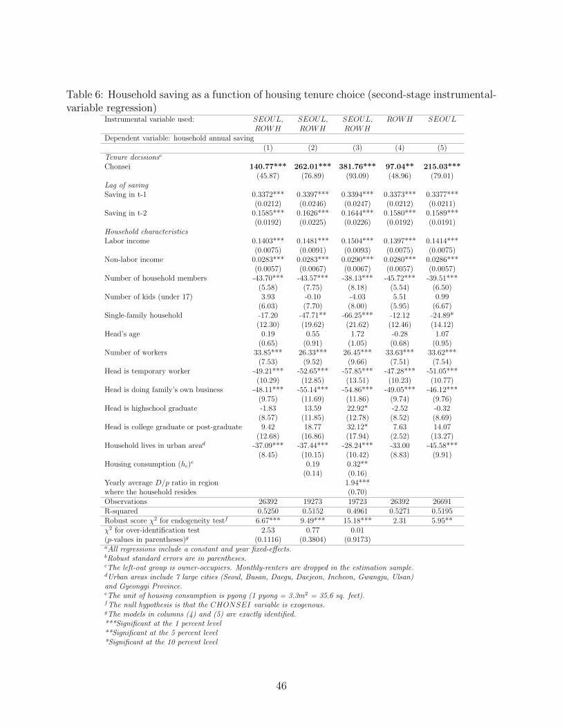
Table 6: Household saving as a function of housing tenure choice (second-stage instrumental-variable regression)
Instrumental variable used: SEOUL, SEOUL, SEOUL, ROWH SEOULROWH ROWH ROWH
Dependent variable: household annual saving(1) (2) (3) (4) (5)
Tenure decisionsc
Chonsei 140.77*** 262.01*** 381.76*** 97.04** 215.03***(45.87) (76.89) (93.09) (48.96) (79.01)
Lag of savingSaving in t-1 0.3372*** 0.3397*** 0.3394*** 0.3373*** 0.3377***
(0.0212) (0.0246) (0.0247) (0.0212) (0.0211)Saving in t-2 0.1585*** 0.1626*** 0.1644*** 0.1580*** 0.1589***
(0.0192) (0.0225) (0.0226) (0.0192) (0.0191)Household characteristicsLabor income 0.1403*** 0.1481*** 0.1504*** 0.1397*** 0.1414***
(0.0075) (0.0091) (0.0093) (0.0075) (0.0075)Non-labor income 0.0283*** 0.0283*** 0.0290*** 0.0280*** 0.0286***
(0.0057) (0.0067) (0.0067) (0.0057) (0.0057)Number of household members -43.70*** -43.57*** -38.13*** -45.72*** -39.51***
(5.58) (7.75) (8.18) (5.54) (6.50)Number of kids (under 17) 3.93 -0.10 -4.03 5.51 0.99
(6.03) (7.70) (8.00) (5.95) (6.67)Single-family household -17.20 -47.71** -66.25*** -12.12 -24.89*
(12.30) (19.62) (21.62) (12.46) (14.12)Head’s age 0.19 0.55 1.72 -0.28 1.07
(0.65) (0.91) (1.05) (0.68) (0.95)Number of workers 33.85*** 26.33*** 26.45*** 33.63*** 33.62***
(7.53) (9.52) (9.66) (7.51) (7.54)Head is temporary worker -49.21*** -52.65*** -57.85*** -47.28*** -51.05***
(10.29) (12.85) (13.51) (10.23) (10.77)Head is doing family’s own business -48.11*** -55.14*** -54.86*** -49.05*** -46.12***
(9.75) (11.69) (11.86) (9.74) (9.76)Head is highschool graduate -1.83 13.59 22.92* -2.52 -0.32
(8.57) (11.85) (12.78) (8.52) (8.69)Head is college graduate or post-graduate 9.42 18.77 32.12* 7.63 14.07
(12.68) (16.86) (17.94) (2.52) (13.27)Household lives in urban aread -37.09*** -37.44*** -28.24*** -33.00 -45.58***
(8.45) (10.15) (10.42) (8.83) (9.91)Housing consumption (hc)
e 0.19 0.32**(0.14) (0.16)
Yearly average D/p ratio in region 1.94***where the household resides (0.70)Observations 26392 19273 19723 26392 26691R-squared 0.5250 0.5152 0.4961 0.5271 0.5195Robust score χ2 for endogeneity testf 6.67*** 9.49*** 15.18*** 2.31 5.95**χ2 for over-identification test 2.53 0.77 0.01(p-values in parentheses)g (0.1116) (0.3804) (0.9173)aAll regressions include a constant and year fixed-effects.bRobust standard errors are in parentheses.cThe left-out group is owner-occupiers. Monthly-renters are dropped in the estimation sample.dUrban areas include 7 large cities (Seoul, Busan, Daegu, Daejeon, Incheon, Gwangju, Ulsan)and Gyeonggi Province.eThe unit of housing consumption is pyong (1 pyong = 3.3m2 = 35.6 sq. feet).fThe null hypothesis is that the CHONSEI variable is exogenous.gThe models in columns (4) and (5) are exactly identified.***Significant at the 1 percent level**Significant at the 5 percent level*Significant at the 10 percent level
46
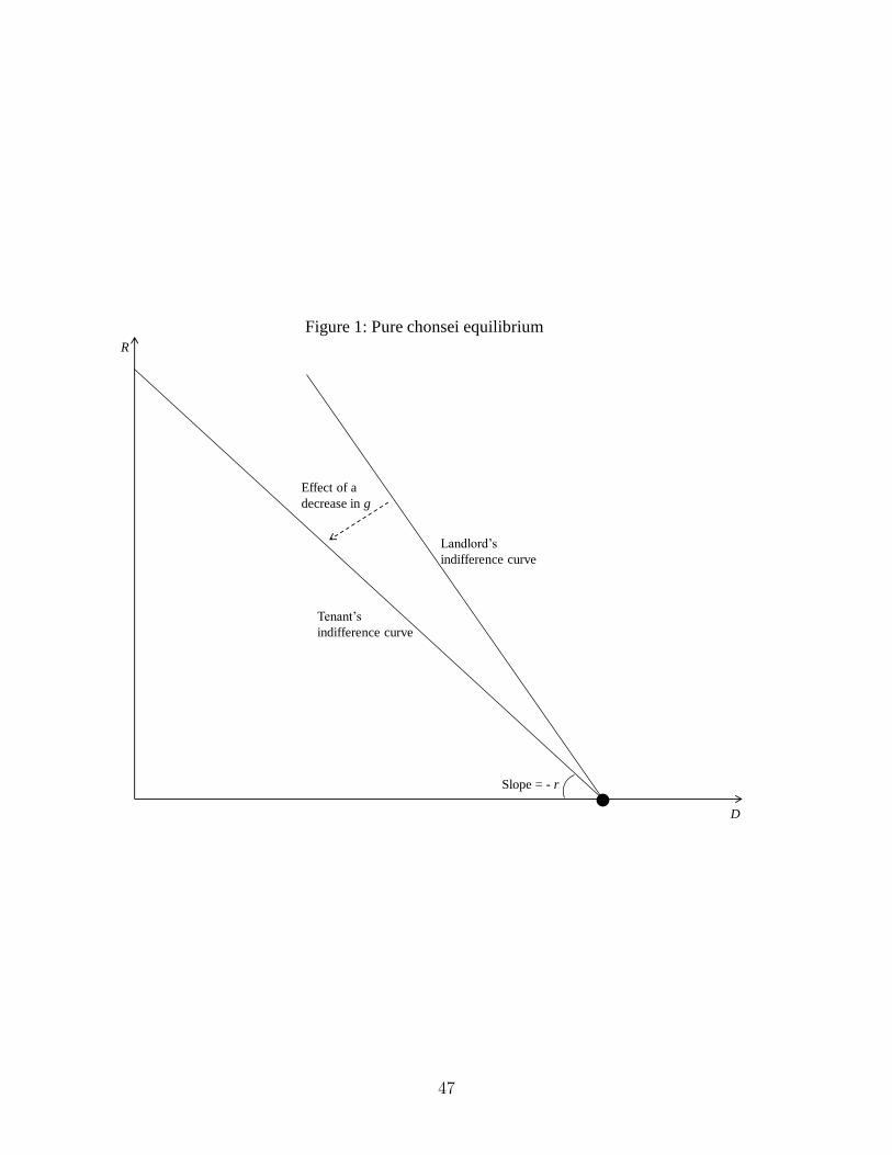
R
D
Tenant’s
indifference curve
Landlord’s
indifference curve
Effect of a
decrease in g
Figure 1: Pure chonsei equilibrium
Slope = - r
47