Embed Size (px)
Citation preview
MPRAMunich Personal RePEc Archive
Elections, Political Competition andBank Failure
Wai-Man Liu and Phong Ngo
Australian National University
26. July 2013
Online at http://mpra.ub.uni-muenchen.de/48689/MPRA Paper No. 48689, posted 30. July 2013 10:30 UTC
1
Elections, political competition and bank failure§
Wai-Man Liu and Phong T. H. Ngo
Australian National University
ABSTRACT
We exploit exogenous variation in the timing of gubernatorial elections
to study the timing of bank failure in the US. Using a Cox proportional
hazard model, we show that bank failure is about 45% less likely in the
year leading up to an election. Political control can explain all of this
average election year fall in the hazard rate. In particular, we show that
the hazard rate for banks operating in states where the governor has
control of both the upper and lower house of the state legislature (i.e.
complete political control) heading into an election falls by
approximately 75%.
JEL Classification: G21, G28, D72, D73
Key Words: bank failure, elections, political competition/control
§ Phong Ngo: College of Business & Economics, Australian National University, Canberra, ACT 0200 Australia; Tel: +61 2 6125 1079; Email: [email protected]. Wai-Man Liu: College of Business & Economics, Australian National University, Canberra, ACT 0200 Australia; Tel: +61 2 61253471; Email: [email protected]. We thank an anonymous referee whose comments have substantially improved this paper. We also thank Aaron Bruhn, Jonathan Brogaard, Lili Dai, Umit Gurun, Michelle Lowry, Terry Walter and seminar participants from the Australian National University and the University of Queensland for helpful comments and discussions. We are grateful to Professor James Snyder for proving us with the U.S. state election data used in an earlier version of this paper.
2
“In Washington, the view is that the banks are to be regulated, and my view is that Washington
and the regulators are there to serve the banks.”
Rep. Spencer Bachus – chairman of the House Financial Services Committee in the 112th Congress1
1. Introduction
The relationship between banking and politics is an intimate one. Governments control
the supply of banks in the economy through chartering restrictions and licensing, they set up
institutions that provide depositors with insurance and banks with a lender of last resort, and
routinely set rules that attempt to govern the risk taking behaviour of banks.
Indeed, according to the bi-annual “Banking Banana Skins” survey by Pricewaterhouse
Coopers and the Centre for the Study of Financial Innovation, “political interference” was rated
as the number one risk that banks faced in 2010.2 Surprising, given the international banking
system had witnessed possibly the worst crisis on record which was largely attributed to credit
and liquidity risks. And ironic given the banks were bailed out by politicians using public
money.
This active role of government in the banking sector creates an incentive problem: on the
one hand, governments play a role in the creation of institutions that make a banking system
possible, while on the other hand they quite often look to the banking system to facilitate their
own political survival. Political support can be indirect, through say, subsidized lending to
preferred industries or direct in the form of campaign contributions or a share of profits due to
ownership. For example, according to the Centre for Responsive Politics, Spencer Bachus, who
is the chairman of the House Financial Services Committee in the 112th Congress, raised over 1 Quoted from an interview with The Birmingham News on 8 December 2010. 2 See http://www.pwc.com.au/media-centre/2010/political-interference-banking-risks-feb10.htm
3
$2.3 million in campaign funds in 2011-2012 with the top five industries being commercial
banks, securities and investment, insurance, real estate and finance/credit companies contributing
over 40%.
So while a healthy banking system can be huge source of benefit for politicians, bank
failure on the other hand, can get politicians into electoral hot water. Politicians therefore have
incentives to interfere with bank closure rules to, for example, favour preferred (politically
connected) constituents or simply to avoid the political costs associated with failure.
There have been several examples in the media of political interference in the banking
system. Probably the most famous case is that of Lincoln Savings and Loans, where five US
senators3 (known as the “Keating Five”) were accused of improperly intervening in a regulatory
investigation of Charles H. Keating, Jr. (Chairman of the Lincoln Savings and Loan Association)
by the Federal Home Loan Bank Board (FHLBB) in 1987. Lincoln Savings and Loans
eventually collapsed in 1989, at a cost of over $3 billion to the federal government. The
substantial political contributions Keating had made to each of the senators, totalling $1.3
million, attracted considerable public and media attention leading to a Senate Ethics Committee
investigation in which three of the senators were found to have “substantially and improperly
interfered with the FHLBB's investigation” and the other two while being cleared were still
criticized for exercising “poor judgement”. All five senators served out their terms however only
two ran for re-election.4
A more recent example is that of Cleveland thrift AmTrust, whose failure was delayed by
11 months because Ohio Congressman Steven LaTourette and Cleveland mayor Frank Jackson
3 Alan Cranston (Democrat of California), Dennis DeConcini (Democrat of Arizona), John Glenn (Democrat of
Ohio), John McCain (Republican of Arizona), and Donald W. Riegle, Jr. (Democrat of Michigan) 4 John Glenn (Democrat of Ohio) and John McCain (Republican of Arizona) were cleared of the charges and re-ran
for office.
4
intervened when the Federal Deposit Insurance Corporation (FDIC) tried to seize and sell the
institution in January 2009.5 By the time AmTrust was finally seized by the FDIC on December
4, 2009 its common equity had fallen by $667 million to $276 million from the year before. The
failure cost the FDIC insurance fund $2 billion.
Are these incidents isolated cases? Or are they representative of a more systematic
phenomenon? A natural place to look for systematic evidence of political interference in
banking is around elections as this is when bank failure can potentially be the most costly to a
politician. Bank failure typically leads to costs that are borne by the local voting population (for
example, due to losses to uninsured depositors, loss of banks jobs etc.), leading the electorate to
question the competency of the incumbent in regulating the banking sector. Accordingly,
politicians have the incentive to take costly action to delay bank failure during election periods.
The economic cost of delay (possibly from larger losses to the insurance fund than would
otherwise be the case) is widespread across taxpayers, whereas the benefits are concentrated with
interest groups like bank owners, employees and uninsured depositors – which further exacerbate
the political incentive to delay bank failure in an election year (see Stigler, 1971; Peltzman,
1976; and Becker, 1983 for more on interest groups).
Our empirical application tests this conjecture using data from the United States (US)
between 1934 and 2012, covering all failed banks (3995) documented by the FDIC.6 We use a
Cox proportional hazard more to exploit the significant cross-state and within-state exogenous
variations in gubernatorial electoral timing to explain the timing of bank failure. A consistent
picture emerges: bank failure is much less likely to occur in the 12 months leading up to an
5 AmTrust was issued with a cease and desist order in November 2008, and when they failed to recapitalise by the deadline of December 31, 2008 the FDIC stepped in. The local politicians were able to delay the failure by convincing Treasury and the White House to keep the FDIC at bay. 6 Note, while our summary statistics include all bank failures between 1934 and 2012, our regression analyses requires accounting data which are only available between 1976 and 2010, covering 1966 bank failures.
5
election than non-election periods. Our results are not only statistically significant but also
economically meaningful. On average, bank failure is approximately 45% less likely in the year
leading up to an election. In contrast, if we categorize the sample of failed banks into banks that
fail outright versus those receiving government assistance, we find that assistance is in fact much
more likely prior to an election whereas outright failure is much less likely. The results are
robust to multiple model specifications and estimation techniques.
We also investigate the role of electoral competition, political patronage and political
control in contributing to the reduction in the election year hazard rate. We measure electoral
competition as the difference in the percentage vote share between the winning candidate and the
second place candidate (i.e. the victory margin) which is a party neutral measure of political
competition. We do not find a statistical relation between political competition and pre-election
year hazard rate; however, the coefficient estimates indicate that competition possibly reduces
the election year fall in the hazard rate. We argue that this result may be due to political
patronage (i.e. politicians favouring electorates where they have strong support) or political
control since control reduces the costs (discussed below) associated with delaying bank failure.7
To measure the partisan support for the incumbent, we calculate the Democrat vote share
across all gubernatorial candidates in any given election and interact it with the party affiliation
of the incumbent governor in an election year. We find evidence that patronage may play a role
– Democrat (Republican) states with Democrat (Republican) governors tend to have an even
larger reduction in the election year hazard rate. However, the exact role of political patronage is
7 A detailed discussion of why costs associated with delaying bank failure are increasing with competition (decreasing with control) is provided in section 4.2. However, briefly, private costs (e.g. those cost incurred if such corrupt behaviour is detected) are increasing since monitoring of the incumbent by the opposition is more effective when political competition is stronger. Also, transactions costs associated with policy making are increasing with competition since competition introduces more veto players (see Tsebelis 1995 and 2002) into the decision making process thereby making it more difficult to implement discretionary decisions like delaying bank failure or providing assistance to failing banks.
6
difficult to disentangle from political control, since states which are heavily Democrat
(Republican) with a Democrat (Republican) governor tend also to be the ones in which the
governor’s party has more control.
To further investigate the role of political control in determining the election year fall in
hazard rate, we construct a variable to capture instances where the incumbent governor’s party
has control (i.e. holds the majority of seats) of both the lower and upper house simultaneously
(i.e. complete control of the state legislature). We show that years in which the governor’s party
has complete political control heading into an election can explain all of the average pre-election
fall in the hazard rate. In particular, our estimates suggest that the hazard rate for banks in states
where the governor has complete control heading into an election falls by approximately 75%.
Our work is related to several streams of literature. First, our work is most related to a
paper by Brown and Dinc (2005) who study electoral incentives to delay bank failure for a
sample of 164 banks (40 of which failed) in developing countries between 1994 and 2000. They
conduct their analysis at the bank level and show that bank failure is much less likely before an
election. Our work complements and extends theirs in several ways. First, a key focus of our
analysis is on political competition and political control and its impact on bank failure during
election years. Second, our study in a US setting provides us with a much larger sample of banks
and a much larger number of failed banks. Moreover, the US setting is useful since the
gubernatorial election cycle is not only exogenous, but also differs both across and within state.8
Third, their analysis is conducted for banks in developing countries where corruption is arguably
8 Not all states hold gubernatorial elections in the same year. Moreover, some states change their constitution and, for example, switch from a 2-year election cycle to a 4-year election cycle during our sample period.
7
more of a problem. In contrast, we study the bank failure in the US – a developed democracy –
and show that political incentives to delay bank failure near elections remain strong.
Second, our work relates directly to the early work arguing that politicians have
incentives to take actions to induce favourable macroeconomic outcomes before elections (see
for example, McRae (1977), Nordhaus (1975) and Rogoff and Sibert, 1988). More recent works
by Levitt (1997, 2002) use election cycles to instrument for the number of police in his study of
the relation between police and crime – arguing that politicians tend to hire more police prior to
elections. Election cycles have also been used recently in the analysis of corporate investment
decisions; Julio and Yook (2012) document a fall in corporate investment corresponding with
timing of national elections around the world.
Third, this paper is related to a broad literature examining various aspects of the political
economy of banking and bank regulation. Earlier work examining the role of politics and the
incentives for regulators to intervene in failing banks’ operations include Kroszner and Strahan
(1996), who show that regulators deferred the realization of costs in failing Savings and Loan
(S&L) associations in the United States. Kroszner and Strahan (1999) also study the political
economy factors that determine the timing of state level relaxation of bank branching restrictions
in the US and find that private-interest (or positive) theory of regulation (Stigler, 1971; and
Peltzman, 1976) best explains the timing of branching deregulation. Rosenbluth and Schaap
(2003) study how electoral rules (centrifugal vs. centripetal) shape the way politicians choose to
regulate their national banking sectors and the resultant impact on market structure. Most
recently, Dam and Koetter (2012) show that political factors determine the likelihood of bank
bailout and therefore bank risk taking (moral hazard).
8
Finally, our paper is related to the large and important debate on the role of political
competition in determining the degree of corrupt behaviour by public officials. Theoretical
studies, for example, by Barro (1973), Rose-Ackerman (1978), Ferejohn (1986), Shleifer and
Vishny (1993); Aidt (2003), Alt and Lassen (2003) conclude that political competition tends to
ameliorate corrupt behaviour. Empirical contributions also find support for the idea that political
competition reduces corruption (see for example, Kunivcova and Rose-Ackerman, 2005;
Lederman et. al., 2005; Tavits, 2007; and Nyblade and Reed, 2008). We also find that political
competition tends to discipline politicians from delaying bank failure, while political control
exacerbates the problem.
The next section discusses the nature of bank failure and bank regulation in the US
context. Section three discusses how the US election cycle works and provides some historical
background on political competition and bank failure in the US. Section four outlines our
empirical approach and presents our results. Section five presents the results from robustness
tests. Finally, section six concludes.
2. Bank failure
The US banking sector is unique in the sense that there are an incredibly large number of
banks, most of which are relatively small. Bank failure is also more frequent relative to other
countries making the US an ideal setting to study bank failure. Data on bank failures and the
characteristics of the failing banks at the time of failure are sourced from the FDIC. The FDIC
has a number of ways in which it deals with a failing institution, so “failure” does not always
imply the bank in question ceases to operate. Broadly, the FDIC categorizes failures into: (1)
9
those in which the bank’s charter survives or “assistance transactions”; and (2) those in which
the bank charter is terminated or “outright failure”. In the case of the former, the FDIC either (1)
provides direct assistance to the failing bank, known as an open bank assistance (OBA)
transaction9; or (2) provides assistance to an acquiring institution to purchase the entire failing
bank. In the case of the latter, the bank charter is terminated and its assets are auctioned off.10 In
what follows we initially consider both assistance transactions and outright failures as the same.
In later analysis, we examine whether the type of failure differs around gubernatorial elections.
Bank regulation in the US is also segmented. While the FDIC insures all deposit taking
institutions, the chartering authority differs depending on whether the institution is a national
bank, a state bank or thrift. The chartering authority for national banks is the Office of the
Comptroller of the Currency (OCC) while states banks are chartered by state regulators.11
Thrifts on the other hand are chartered by the Office of Thrift Supervision (OTS) which is a
federal agency.12
Panel A in Table 1 presents a summary of all failed banks. In total, there have been 3995
bank failures in the US between 1934 and 2012. Not surprisingly, these have been concentrated
(2822 failures) in the two major crises since the great depression: the S&L crisis, 1986-1992 and
the recent Global Financial Crisis (GFC), 2007-2010. As we will discuss below, appropriately
controlling for these crises is very important for our analysis. Failures are also concentrated in
the Southern states where almost half (1979) of the failures were recorded. Of the failures, 2528 9 OBA transactions were popular leading into and during the S&L crisis but lost their lustre following the passage of Financial Recovery, Institutions Reform and Enforcement Act (FIRREA) of 1989 and the FDIC Improvement Act (FDICIA) of 1992. The FDICIA in particular made it more difficult for the FDIC to provide assistance to failing banks unless it could: (1) demonstrate that this would minimize the cost to the insurance fund or; (2) show that the closure of the failing bank will increase the risk of systematic failure (Mingo, 1994). 10 For more detail on FDIC transaction types see: http://www2.fdic.gov/hsob/help.asp 11 Supervision is carried out by the FDIC in the case of state banks while the Federal Reserve supervises national banks as well as state banks electing to be members of the Federal Reserve System. 12 The OTS was dissolved on July 2011 and its powers transferred to the OCC.
10
were commercial banks (815 with national charters and 1713 state chartered) and 1467 were
thrifts. In terms of the two broad categories of FDIC failure transactions, unlike Brown and Dinc
(2005), most of the failures in our sample are outright failures whereby the banks charter is
terminated and it ceases to operate – only 593 of the 3995 failures are assistance transactions
where the bank’s charter continues. Since our regression analysis below requires bank
accounting data which are only available from 1976, we also report a summary of the failed bank
sample for banks failing from 1976 onwards in the bottom half of Panel A. The distribution of
bank failures is largely the same as described for the full sample. Briefly, 3473 of the 3995
failures occurred between 1976 and 2012. Of these failures, 719 are national banks, 1289 are
state banks, 591 are assistance transactions and 2882 are outright failures.
3. Elections in the US
Election timing in the US is exogenously determined by law. Since 1845, Election Day
occurs on the Tuesday in November after the first Monday – so Election Day must fall
somewhere between November 2 and November 8 (inclusive). Presidential elections follow a
four year cycle on even numbered years. Other federal offices (House of Representatives and
Senate) run on a two year cycle on even numbered years (i.e. on presidential election years as
well as mid-term elections).
At the state level, most states choose to run their gubernatorial elections in the same years
at the federal elections (i.e. gubernatorial elections coincide with either presidential or mid-term
elections). Only five states run their gubernatorial elections in “off-years” or odd-numbered
11
years.13 In all but the states of New Hampshire and Vermont, gubernatorial elections currently
follow a four year cycle.14
For example, consider the Ohio General Assembly which is the state legislature of the US
state of Ohio.15 State election years coincide with federal midterm elections (i.e. 2010, 2014,
2018, 2022, etc.) – election day involves electing: Governor, Lieutenant Governor, Secretary of
State, Treasurer of State, Auditor of State, Attorney General, State Senators (odd-numbered
districts), State Representatives, State Board of Education (one-third of members), Supreme
Court Justices (two or three) and some county officials.16 In some cases, states have changed the
length of their gubernatorial election cycle. For example, in 1986 the state of Arizona changed
from holding gubernatorial elections every two years to every four years.
Accordingly, unlike presidential elections, there are substantial across and within state
variations in the timing of gubernatorial elections. We exploit this exogenous variation in
gubernatorial election timing to study whether bank failure can be explained by electoral
concerns.17 Since we are focusing on gubernatorial elections, the relevant financial institutions
we are interested in are state banks whose charters are controlled by state authorities. While
thrifts and nationally chartered banks are not the focus of the main analysis, they are included in
our summary statistics for a more complete picture.
13 These are Kentucky, Louisiana, Mississippi, New Jersey, and Virginia 14 These two states hold gubernatorial elections every two years. 15 It consists of the 99-member Ohio House of Representatives and the 33-member Ohio Senate. Both houses of the General Assembly meet at the Ohio Statehouse in Columbus. 16 Other state races such as those for State Senators (even-numbered districts), State Representatives, State Board of Education (one-third of members), Supreme Court Justices (two or three) and remaining county officials are held on Presidential election years (2012, 2016, 2020, etc.). State election days also involve electing the federal offices of: the President of the United States, U.S. Senators (if term expires), and Representatives to Congress. 17 In additional tests, we also examine the impact of Presidential elections for federally charted banks.
12
Let the election date be day 0, we report in Table 1 the frequency of bank failure for a 24
month period around day 0 (i.e. 12 months prior to and 12 months after an election) as well as
the failures that fall outside this 24 month window. As mentioned previously, since a number of
states either currently or historically hold gubernatorial elections every two years we choose the
[12, +12] window since this is the longest possible window around a gubernatorial election that
does not crossover into elections preceding and following it.
If we compare the number of failures that occur in the 12 months prior to an election date
to the number that occur in the 12 months following an election date, we find that (for the full
sample) 941 failures occur in the 12 months leading up to a gubernatorial election while 963
failures occur in the 12 months following. The remaining 2091 failures fall outside our [-12,
+12] window.18
While these data show that there are fewer bank failures in the 12 months prior to an
election compared to the 12 months after, the difference is not meaningful. Further investigation
shows that failures clustered in crises periods tend to coincide with the pre-election period. To
see this, we sub-divide the sample into crisis periods (i.e. the S&L Crisis 1986-1992 and the
Global Financial Crisis 2007-2010) versus non-crisis periods (i.e. all other years). The second
column of Panel A in Table 1 shows that in crisis years, 705 failures occur in the 12 months
leading up to an election while only 577 occur in the 12 months following. We argue that there
are several reasons why we should concern ourselves predominantly with investigating political
incentives to delay failure in non-crisis years. First, during a crisis, the political cost to a local
18 Note that the failures occurring outside our [-12, +12] window (i.e. “Not around election” rows) are not directly comparable with the [-12, 0] and [0, +12] failure counts. For states with a two year gubernatorial election cycle, then by definition, banks will fail either before or after an election. However, for states with a four year election cycle, the “Not around election” period represents a 24 month period – so the failure count would have to be divided by two to be comparable our pre- and post-election windows. In our regression analysis, this “Not around election” period represents our benchmark.
13
politician associated with a bank failure is lower since he can – in part or in full – deflect the
cause of the failure away from his potential mismanagement of the economy and bank
regulation. Second, bank failure tends to be more severe during a crisis which accordingly
makes it more difficult for politicians to delay regulatory intervention, other things equal. These
differing incentives during a crisis imply we are much less likely to observe political factors
determining bank failure.
Looking at the third column of Table 1 Panel A, we see that in non-crisis periods, 236
failures occur in the 12 months prior to an election whereas 386 fail in the 12 months after.
These data imply that the frequency of bank failure is almost 40% lower in the 12 months before
an election compared to the 12 months after. These findings are best illustrated in Figure 1.
Here, the blue bars plot the number of bank failures in 3-month blocks leading up to an election
while the pink bars plot the number of bank failures in 3-month blocks in the months after state
elections. The blue and pink horizontal dashed lines represent the average number of bank
failures in a 3-month period before and after elections respectively. Figure 1a plots bank failure
for all years between 1934 and 2012 while Figure 1b plots bank failure around elections only for
non-crisis years – that is, failures that occur during the S&L Crisis (1985-1992) and the Global
Financial Crisis (2007-2010) are excluded.
While Figure 1a shows no discernible difference between the pre- and post-election
failure rates (235 vs. 240 failures per 3-months respectively), a striking picture emerges when we
control for the clustering of bank failure around crises: bank failure is much less likely in the
months leading up to an election than in the months after. For the non-crisis period, the pre- and
post-election average number of bank failures are 59 and 97 failures per three-months
respectively. Therefore, based on raw numbers alone, bank failure is about 40% less likely in the
14
months leading up to an election compared to the months following an election. This finding
highlights the importance of properly controlling for impact of financial crisis. The pattern
described above is largely consistent for our subsamples. Looking further down column 3 of
Panel A in Table 1 and comparing failures in the pre-election period to the post-election we find
that failure is 53% less frequent for all commercial banks (151 failures pre- vs. 323 failures post-
election), 57% less frequent for state charted banks (115 failures pre- vs. 267 failures post-
election), 30% less frequent for all banks and thrifts in the 1976-2012 period (145 failures pre-
vs. 206 failures post-election), 58% less frequent for commercial banks in the 1976-2012 period
(60 failures pre- vs. 143 failures post-election), and 63% less frequent for state chartered banks
in the 1976-2012 period (43failures pre- vs. 117 failures post-election).
Up to this point, we have used the term bank failure to mean both outright failures where
banks lose their charter and cease to operate as well as FDIC assistance transactions where a
failing institution is restructured with FDIC assistance and allowed to continue to operate under
its existing charter. As a first attempt to examine whether political concerns determine the type
of failure transaction chosen by regulators around elections we split all failures into two
subsamples depending on the failure type. For the 1934-2012 non-crisis sample (column 3 of
Table 1 Panel A) we see that outright failures are about 55% less frequent in the months leading
up to an election compared to the months following (154 failures pre- versus. 339 failures post-
election). However, interestingly, we find that FDIC assistance transactions are much more
likely in the months leading into an election. Based on our raw data, assistance is almost 75%
more likely to occur in the 12 months leading up to an election (82 failures pre- versus 47
failures post-election). It appears as though an alternative to delaying outright bank failure,
politicians can also opt to provide assistance to failing banks so that they can continue to operate
15
in the year leading up to an election. In Figure 2 we plot the frequency of bank failures around
elections separately for outright failures (Figure 2a) and assistance transactions (Figure 2b). Like
Figure 1 the blue bars plot the number of failures in 3-month blocks leading up to an election
while the pink bars plot the number of failures in 3-month blocks in the months after elections.
The blue and pink horizontal dashed lines represent the average number of bank failures in a 3-
month period before and after elections respectively. There is a remarkable difference between
the two figures: outright failures are clearly less frequent prior to elections whereas assistance is
much more frequent.
[INSERT TABLE 1, FIGURES 1 AND 2 HERE]
4. Empirical strategy and results
This section describes our empirical approach and presents the results from our analysis.
We obtain quarterly accounting data for all (failed and surviving) commercial banks operating in
the US from bank call reports filed with regulators. These data are available from March 31,
1976 till December 31, 2010. We hand collect political data on the election dates and outcomes,
the composition of state legislatures, party affiliation of governor and so on from the Census
Bureau Statistical Abstracts.19 State macroeconomic data are sourced from the Bureau of
Economic Analysis and Bureau of Labour Studies. Our final sample of banks for which
accounting data are available is an unbalanced panel of 22230 banks, of which 1966 fail.
Let the election date for state j be day 0, we construct a PRE-ELECTION variable that
equals one if accounting quarter t of bank i from state j falls in the [-12, 0) month window, and
19 See: http://www.census.gov/compendia/statab/cats/elections.html. These data are also verified using internet sources such as http://www.ourcampaigns.com/
16
zero otherwise. Likewise, we construct a POST-ELECTION variable that equals one if
accounting quarter t of bank i from state j falls in the [0, +12] month window, and zero
otherwise. We test whether bank failures, defined as an outright failure or assistance transaction,
do not depend on the gubernatorial election cycle in a Cox proportional hazard model given by20
h(t) = exp(β'X it + γ1PRE-ELECTIONit + γ2POST-ELECTIONit + θt + θj) (1)
for t = ti, …, Ti, where ti and Ti represent bank i’s entry and exit dates (quarter) respectively. In
particular, the following entry and exit dates are used for the analysis. Bank i enters the study in
quarter ti, which is the later of two possible dates: (1) March 31, 1976 (the start of the sample
period); or (2) the date bank i files its first call report after receiving its charter. Bank i exits the
study in quarter Ti, which is the earliest of four possible events: (1) the banks fails (outright) and
its charter is terminated; (2) the failing bank receives FDIC assistance, is restructured and
allowed to continue to operate under its existing charter; (3) the bank is acquired by another bank
so balance sheet data are no longer available for that bank as a separate entity; or (4) the bank
survives until December 31, 2010 (the end of the sample period). In what follows, exit scenarios
(1) and (2) are both considered as bank ‘failure’ unless we explicitly distinguish between the two
in our discussion.
Here X it is a vector of bank level and state level controls, θt is a year fixed-effect to
control for common time effects such as crises and θj is a state fixed-effect. State
macroeconomic controls (important for appropriately controlling for crises) include: (1)
GROWTH which is annual state personal income growth; and (2) BUDGET DEFICIT, defined
as the ratio of total state taxes less total state government expenditure to gross state product.
Bank level controls include standard predictors of bankruptcy: (1) SIZE, defined as the natural
20 See Shumway (2001) for a discussion of forecasting bankruptcy using hazard models.
17
log of total deposits; (2) INCOME/ASSETS RATIO, (i.e. return on assets) defined as net income
to total assets; (3) CAPITAL RATIO, defined as total equity capital to total assets; and (4) NPL,
defined as non-performing loans as a percentage of total loans. Recent policy discussions have
emphasized the importance of ‘too big to fail’ in determining bank failure and risk taking,
accordingly, we also include the variable TOO BIG TO FAIL defined as a bank’s assets at
quarter t as a percentage of total banking assets in state j at quarter t. Finally, Brown and Dinc
(2011) provide evidence from developing countries that a government is less likely to takeover
or close a failing bank if the banking system is weak. To capture the possibility of a ‘too many
to fail’ effect we include in our regressions the variable TOO MANY TO FAIL defined as the
average capital ratio of all other banks in state j.21
Panel B in Table 1 presents summary statistics for state controls.22 State income growth
averaged 7% for the entire sample and is lower (6%) for states in the North East and Mid-West.
States run persistent government deficits, averaging 2%, with states in the West having the
largest deficits of 3% on average. Panel C in Table 1 presents summary statistics for bank level
controls for the full sample as well as for the subsamples of failed banks (outright failure and
assistance transactions separately) and all other banks. As expected, failed banks are routinely
less profitable, have higher non-performing loans and lower capital ratios than banks that do not
fail. Of the failed banks, those receiving FDIC assistance tend to be slightly better performing
on these three measures compared to banks failing outright. Banks failing outright tend to be
slightly smaller than non-failing banks ($45 million versus $46 million total deposits), however,
banks receiving assistance are significantly larger than both banks failing outright and surviving
21 We also use alternative proxies for TOO BIG TO FAIL, namely, (1) the average percentage of NPL of all other banks in state j; and (2) the average income to assets ratio of all other banks in state j and find similar results (not reported). 22 The regression sample period is 1976-2010 (inclusive).
18
banks with an average deposit base of approximately $109 million. Indeed, if we examine state
market shares – our proxy for ‘too big to fail’ – we see that banks failing outright control less
than 0.3% of state banking assets (almost 0.5% for surviving banks) compared to 2.1% for banks
receiving FDIC assistance. This evidence hints at the possibility of there being a ‘too big to fail’
effect in US bank closure policy: larger banks controlling a larger fraction of banking assets tend
to receive assistance rather than having their charters terminated by regulators. Finally,
comparing our TOO MANY TO FAIL variable across our three categories of banks we find that
the average capital ratio of other banks is slightly lower for failing banks than surviving banks
(9.0% vs. 9.9%) which is inconsistent with the conjecture that regulators tend to close banks
when the banking system is stronger. For banks receiving assistance, the average capital ratio of
other banks is 8.8% which is lower than the case for outright failure. Consistent with the ‘too
many to fail’ hypothesis, when the banking sector is weak, regulators prefer to provide assistance
as opposed to closing a bank. So while the evidence on ‘too many to fail’ is somewhat mixed,
our summary statistics do suggest the possibility of regulatory forbearance when the banking
sector is weak, where forbearance comes in the form of providing assistance to larger and more
systematically important institutions.
4.1. Elections and bank failure
The main regression results are reported in Table 2. All regressions include state fixed-
effects as well as year fixed-effects to control for common state and time factors. Standard
errors are robust to heteroscedasticity and clustering at the state level. Regression models 1-4
include only the PRE-ELECTION dummy, whereas models 5-8 include both the PRE-
ELECTION and POST-ELECTION dummies. Regression models 1, 2, 5 and 6 are performed
on the full sample of banks (i.e. federally chartered and state chartered banks) whereas models 3,
19
4, 7 and 8 use only state chartered banks. Odd numbered regression models include only
standard bank level predictors of failure: INCOME/ASSETS, SIZE, CAPITAL RATIO, and
NPL. Even numbered models include the bank level controls mentioned above, TOO BIG TO
FAIL and TOO MANY TO FAIL variables as well as macroeconomic controls.
A consistent picture emerges: in all specifications, the coefficient on PRE-ELECTION is
negative suggesting that bank failure is less likely in the year leading up to a gubernatorial
election. As discussed earlier (and illustrated in Figure 2) controlling for the impact of financial
crisis is crucial to our analysis since failures tend to cluster around crises. While some of the
impact of crises is accounted for in our time and state fixed effects, it is clear that our results are
much stronger when time varying macroeconomic controls are added into our specification.
Indeed, the pre-election effect is significant in all but models 1 and 3 where we do not include
the POST-ELECTION dummy, too big/too many to fail variables and macroeconomic controls.
Results are also stronger for our sample consisting only of state chartered banks – which makes
sense given we are studying the impact of gubernatorial elections, so the relevant regulatory
jurisdiction is at the state level. To give an indication of the economic significance of this pre-
election effect, the coefficient for state chartered banks is approximately -0.57 which translates
to a reduction in the probability of failure by about 45% in the year leading up to an election. For
the full sample, the PRE-ELECTION coefficient of -0.43 translates into a 35% reduction in the
probability of failure. Interestingly, in all of our baseline regressions, the POST-ELECTION
variable cannot explain bank failure as they are insignificantly different from zero.23
23 In comparison, Brown and Dinc (2005) show for their sample of developing country banks that there is a decrease in the hazard rate by about 70% in the year leading up to an election.
20
Across all specifications, INCOME/ASSETS, SIZE and CAPITAL RATIO are
negatively related to bank failure whereas higher NPL increases the likelihood of failure. These
results are expected and in line with previous studies. Our macroeconomic controls also provide
results consistent with expectations. Higher state income growth reduces the likelihood of bank
failure, with the effect being stronger for and significant for the regression models using the state
chartered banks only (models 4 and 8). This is not surprising given federally chartered banks are
usually larger and more diversified across state boarders making them less sensitive to changes
in local economic conditions. To the extent that delaying bank failure involves some fiscal costs,
one might expect a positive relation between BUDGET DEFICIT and bank failure since that
states with larger budget deficits are less able to influence the timing of bank failure. Consistent
with our conjecture the variable BUDGET DEFICIT is positively related to bank failure,
however insignificant. Our TOO BIG TO FAIL variable is positive and significant across all
specifications. This might at first seem counterintuitive, however, recall: (1) for our hazard
analysis, we define failure to be either outright failure or FDIC assistance; and (2) from our
summary statistics, larger banks with a bigger market share are more likely to receive FDIC
assistance. To confirm that this positive coefficient on TOO BIG TO FAIL is driven by the
assistance banks we re-estimate the regression models in Table 2 (not reported) redefining failure
to be outright failure only and find that the coefficient on TOO BIG TO FAIL is negative and
significant, consistent with the view that regulators are less willing to close banks that are
‘systematically important’.24 Finally, unlike Brown and Dinc (2011) we find no evidence of a
‘too many to fail’ effect in our sample of US banks once we control for the ‘too big to fail’ effect
and the macroeconomic environment. For the remainder of the paper, we indicate which control
variables we use in our specifications but do not report the coefficient estimates to preserve 24 All other coefficient estimates remain virtually unchanged when defining failure as outright failure only.
21
space. Moreover, the coefficient estimates for our control variables remain largely unchanged
for our various specifications.
[INSERT TABLE 2 HERE]
Before moving on, we re-estimate our baseline regressions presented in Table 2 using
alternative methods to ensure our results are robust to estimation technique. We employ three
alternative estimation techniques: (1) linear probability model; (2) dynamic logit model; and (3)
the exponential proportional hazard model used in Brown and Dinc (2005). The linear
probability model and logit model are discrete models where the dependent variable equals one
in the quarter a bank fails and zero otherwise whereas the difference between the Cox and
exponential proportional hazard models is that the Cox model leaves the unconditional survival
function unspecified whereas survival is assumed to follow an exponential distribution in the
case of the latter. The results are presented in Table 3 in two panels. Panel A re-estimates our
baseline regressions with only PRE-ELECTION variable (i.e. models 1-4 in Table 2) while Panel
B re-estimates our baseline regressions when we include both PRE-ELECTION and POST-
ELECTION variables (i.e. models 5-8 in Table 2). In both panels, regression models 1-4
represent estimates from the linear probability regression, models 5-8 are obtained from the logit
regression, and models 9-12 from the exponential hazard. We find consistent results from all
three estimation techniques. First, the estimates from the exponential hazard model are virtually
identical to those obtained from our Cox regression save that the coefficients are statistically
more significant. Second, the results from the logit model are again similar to those obtained
from the Cox regressions, however, the magnitudes of the coefficient estimates are larger
implying a reduction in the hazard rate by about 60% in the year leading up to an election.
Similar to the Cox model, the POST-ELECTION variable is insignificant in the logit and
22
exponential models once a full list of controls is added. Finally, our linear probability estimates
also confirm the reduction in hazard rate in the year before an election. The point estimates
range between -0.0002 and -0.0003. When compared to the unconditional failure rate of
0.00123, these estimates imply a reduction in failure rate by between 15% and 25%. However,
unlike the other models, the coefficient on POST-ELECTION is negative and significant in all
specifications and is of approximately the same magnitude as the PRE-ELECTION coefficient
implying that the hazard rate remains about 15-25% lower after an election in comparison to
non-election periods. It is interesting to note that the linear probability model predicts a
reduction in the failure rate of up to 50% in the 24 months around an election, however, evenly
split over the pre- and post-election period whereas our non-linear models predict a reduction in
the hazard rate of a similar order of magnitude over a 24 month period, however, the reduction
occurs in the 12 months leading up to an election with little effect found in the post-election
period.
[INSERT TABLE 3 HERE]
In sum, the results in Tables 2 and 3 provide evidence supporting the view that electoral
concerns drive politicians to take costly action to delay bank failure in an election year. We do
not find evidence of a post-election increase in the hazard rate as suggested might be the case in
the summary statistics – we investigate this further in the following section. In particular, in the
remaining sections, we will investigate the role of political competition and political control in
magnifying or attenuating this pre-election reduction in the hazard rate.
23
4.2. Political competition and bank failure
The costs associated with bank failure; such as losses to uninsured depositors, bank job
losses, and potential reductions in local economic activity are likely to be concentrated in the
state where the bank operates. Accordingly, political support for the incumbent party in that
state may decrease because of these costs. Moreover, if the incumbent and opposition parties
have similar levels of voter support, the impact of the voter backlash is likely to be stronger.
Political (electoral) competition therefore increases the benefit to politicians from delaying bank
failure and therefore we might expect that elections that are closely contested exacerbate the pre-
election reduction in the hazard rate, ceteris paribus. To measure the extent of political
competition, we construct a variable similar to Dinc and Gupta (2011) to measure the closeness
of the election. In particular, our party neutral measure, VICTORY MARGIN, is defined as the
difference between the winning candidate’s vote share and the second place candidate’s vote
share – smaller values are associated with stronger political competition.25 The summary
statistics in Panel B of Table 1 show that gubernatorial elections post-1976 are on average not
very competitive, with the average victory margin of 17%. There is, however, significant
variation in this measure with a standard deviation 14%.26 Southern states are marginally less
competitive with an average victory margin of 18%.
25 In an earlier version of this paper, we used the party neutral measure of political competition developed in Besley et al. (2010). Their measure uses data originating from the work of Ansolabehere and Snyder (2002), who collected election results for a broad set of directly elected state executive offices. These elections range from US representatives, over the governorship, to down-ballot officers, such as Lieutenant Governor, Secretary of State, Attorney General, and so on. We thank James Snyder for generously providing us with an updated version of this data which was used in our earlier work. 26 These summary statistics based on a post-1976 sample hide some of the substantial variation in political competition over time in the US – in particular in the US Southern states in the first half of the 20th century. By the 1880s, the Democrats held a virtual monopoly over political office in the US Southern states. They achieved this by limiting the political participation of the black and low income population which made up the supporter base of their main rivals – the Republicans. Several voting restrictions were introduced over the years including: the white primary, multiple ballot boxes, poll taxes, literacy tests, and ultimately violence. This effectively eliminated
24
In our empirical application, we construct two dummy variables: HIGH VICTORY
MARGIN (i.e. low competition) and LOW VICTORY MARGIN (i.e. high competition) equal to
one for elections with victory margins in the top and bottom quartile respectively.27 We are
interested in the coefficient estimate on the interaction term between these two dummy variables
with our PRE-ELECTION variable. From our previous discussion, we expect that if higher
competition exacerbates the political incentive to delay bank failure then the coefficient on the
interaction between PRE-ELECTION and HIGH VICTORY MARGIN (LOW VICTORY
MARGIN) to be positive (negative). The results are presented in Table 4. The first four
regression models employ the HIGH VICTORY MARGIN variable whereas the last four models
employ the LOW VICTORY MARGIN variable. Regression models 3, 4, 7 and 8 also include
an additional control variable DEMOCRAT GOVERNOR, which is equal one when the
governor is a democrat.
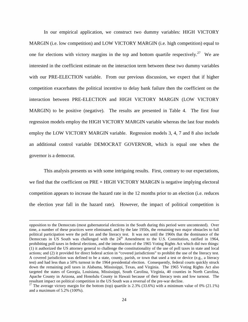
This analysis presents us with some intriguing results. First, contrary to our expectations,
we find that the coefficient on PRE × HIGH VICTORY MARGIN is negative implying electoral
competition appears to increase the hazard rate in the 12 months prior to an election (i.e. reduces
the election year fall in the hazard rate). However, the impact of political competition is
opposition to the Democrats (most gubernatorial elections in the South during this period were uncontested). Over time, a number of these practices were eliminated, and by the late 1950s, the remaining two major obstacles to full political participation were the poll tax and the literacy test. It was not until the 1960s that the dominance of the Democrats in US South was challenged with the 24th Amendment to the U.S. Constitution, ratified in 1964, prohibiting poll taxes in federal elections, and the introduction of the 1965 Voting Rights Act which did two things: (1) it authorized the US attorney general to challenge the constitutionality of the use of poll taxes in state and local actions; and (2) it provided for direct federal action in “covered jurisdictions” to prohibit the use of the literacy test. A covered jurisdiction was defined to be a state, county, parish, or town that used a test or device (e.g., a literacy test) and had less than a 50% turnout in the 1964 presidential election. Consequently, federal courts quickly struck down the remaining poll taxes in Alabama, Mississippi, Texas, and Virginia. The 1965 Voting Rights Act also targeted the states of Georgia, Louisiana, Mississippi, South Carolina, Virginia, 40 counties in North Carolina, Apache County in Arizona, and Honolulu County in Hawaii because of their literacy tests and low turnout. The resultant impact on political competition in the US South was a reversal of the pre-war decline. 27 The average victory margin for the bottom (top) quartile is 2.3% (33.6%) with a minimum value of 0% (21.1%) and a maximum of 5.2% (100%).
25
statistically insignificant. Second, the coefficient on PRE × LOW VICTORY MARGIN is also
negative. While this is more in line with our expectations, the coefficient estimates are again
insignificant. Third, after controlling for political competition, we find that our POST-
ELECTION variable becomes positive and statistically significant in all specifications. This is
consistent with our summary statistics, suggesting the reduction in the failure rate in the 12
months before an election is followed by a substantial increase in the bank failure rate in the 12
months after. Fourth, the positive and significant coefficients of POST × HIGH/LOW
VICTORY MARGIN seem to indicate that both very competitive and very uncompetitive
elections are associated with a bigger post-election increase in the hazard rate. Fifth, the
coefficient estimates on our PRE-ELECTION variable are larger in magnitude. For state
chartered banks (models 2, 4, 6 and 8), the coefficient on PRE-ELECTION implies a reduction
in the hazard rate of about 55% in the 12 months leading up to an election. Finally, the
coefficient on our democrat governor indicator is negative, and also significant.
[INSERT TABLE 4 HERE]
Our mixed and insignificant electoral competition results are, on face value, surprising.
However, while we argued earlier that the benefit of delay to the politician is increasing with
political competition, there are at least two reasons as to why we might observe a larger
reduction in the pre-election hazard rate for more competitive elections – meaning the net effect
is an empirical matter.
First, a negative relation between political competition and incentives delay may exist
due to political patronage – the idea that rent seeking politicians tend to make decisions to
reward supporters (see Cox and McCubbins, 1986; and Persson and Tabellini, 2002). Note that
26
Ansolabehere and Snyder (2007) argue that it is possible that politicians may target both areas
that support them as well as politically competitive areas. Previous evidence of political
patronage include Ansolabehere and Snyder (2007) who show governing parties provide more
public funds to regions that support them, and Dinc and Gupta (2011) who show that politicians
do not privatize firms located in the state from which a minister with jurisdiction over that firm is
elected.
Second, it is likely that the costs of delay are also increasing with political competition.
Private costs associated with delay are those incurred in the event such corrupt behaviour is
detected. There have been numerous studies looking at the cost of corruption charges on
politicians’ subsequent electoral performance (e.g. Alford et. al., 1994; Jacobsen and Dimock,
1994; and Peters and Welch, 1980) and politicians’ decisions to retire (e.g. Groseclose and
Krehbiel, 1994; and Hall and Van Houweling, 1995).28 These costs can be increasing with
competition for several reasons. First, political competition increases the likelihood that any
corrupt behaviour by incumbent politicians is detected since opposition parties are either more
numbered and/or more incentivized to monitor the actions of the incumbent lending into an
election. Rising private costs to the politician reduces their incentive to delay bank failure.
More broadly, this idea is related to the large debate on whether political competition reduces
corruption. In general, this literature suggests that competitive elections serve as a disciplining
role against corruption.29
28 Indeed, three of the five “Keating Five” senators retired following an investigation into their interference in the FDIC investigation of Charles Keating, the chairman of Lincoln S&L. These were Alan Cranston (Democrat of California), Dennis DeConcini (Democrat of Arizona), and Donald W. Riegle, Jr. (Democrat of Michigan). 29 See studies by Barro (1973), Rose-Ackerman (1978), Ferejohn (1986), Shleifer and Vishny (1993); Aidt (2003), Alt and Lassen (2003) for theoretical contributions. Empirical contributions also support the idea that political competition reduces corruption; see for example, Kunivcova and Rose-Ackerman (2005), Lederman et. al. (2005); Tavits (2007); and Nyblade and Reed (2008).
27
The second condition influencing the cost of delaying bank failure are the transactions
costs associated with decision making. As political competition increases, more actors are
involved in the decision-making process and as more decision points must be crossed,
transactions costs increase. These kinds of transactions costs are often referred to as veto points
(Tsebelis 1995 and 2002). More veto points make policy commitments more credible (i.e.
irreversible), but they also make them more costly and time-consuming to implement and
change. To the extent that bank closure policy is more credible in states-years with more veto
players, we expect political competition to reduce the ability of incumbent politician’s ability to
make discretionary policy decisions like delaying bank failure. Evidence of the important role of
veto players in economic policy making can be found in Keefer and Stasavage (2003), who study
the role of veto players on the degree of central bank independence and subsequent credibility
(i.e. effectiveness) of monetary policy. The authors show that rising veto players enhances
central bank independence by reducing the time inconsistency of monetary policy and also
reduces central bank governor turnover.30
The next section of the paper investigates the possibility of patronage and/or costs (both
private and transactions costs determined by the degree of political control) of delay in driving
our election year results. Note however, that while both hypotheses predict competition reduces
the fall in the election year hazard rate, it is difficult to disentangle their separate effects.
30 Their measure of veto players is based on whether the executive and legislative chamber(s) are controlled by different parties in presidential systems and on the number of parties in the government coalition for parliamentary systems. The indicator rises with the number of veto players (depending upon the number of legislative chambers) and falls when the veto points are occupied by the same political party (depending on whether majorities are multiparty coalitions). The index is then modified to take account of the fact that certain electoral rules (closed list vs. open list) affect the cohesiveness of governing coalitions.
28
4.3. Patronage, political control and bank failure
4.3.1. Political patronage
We begin by investigating the potential role of patronage in driving the election year fall
in the hazard rate. For this, we first create a variable which captures how much support a
particular party (Democrat or Republican) has in a given state for a given election period. We
calculate the DEMOCRAT VOTE SHARE as the vote share across all gubernatorial candidates
affiliated with the Democrat party in any given election. The summary statistics in Table 1 Panel
B show that the average Democrat share across all states for our sample period is 49%. There is
significant variation in the Democrat vote share with a standard deviation of 14%. For our
regression analysis below we construct two dummy variables HIGH DEM SHARE and LOW
DEM SHARE which equal to one if DEMOCRAT VOTE SHARE is in the top and bottom
quartiles respectively. HIGH DEM SHARE is designed to capture heavily democrat states while
LOW DEM SHARE captures heavily republican states. The mean democrat vote shares for our
indicators HIGH DEM SHARE and LOW DEM SHARE are 64% and 33% respectively.
We are interested in seeing whether an incumbent governor is more or less likely to delay
bank failure in an election year if he is in a state which strongly supports his political party. In
particular, we are interested in determining whether a Democrat (Republican) governor in a
Democrat (Republican) state is more or less likely to delay bank failure in an election year
compared to the same governor in a Republican (Democrat) state. We create interaction terms
between our variables HIGH DEM SHARE and LOW DEM SHARE with an indicator for
governor party affiliation (either DEM GOV or REP GOV) and our PRE/POST-ELECTION
29
variables. Table 5 presents the results from our regression analysis.31 Regression models 1-4
present results using an indicator for when the incumbent governor is a Democrat while models
5-8 replaces the Democrat governor indicator with a Republican governor indicator.
The coefficient on the interaction term PRE × DEM GOV × HIGH DEM SHARE is
negative and significant in both specifications (models 1 and 2) suggesting that the election year
reduction in hazard rate is exacerbated in instances where there is an incumbent Democrat
governor operating in a heavily Democrat state. The inclusion of this interaction term reduces
the magnitude and significance of the coefficient on PRE-ELECTION compared to estimates
using party-neutral measures of competition in the previous section. This suggests that the pre-
election fall in hazard rate can be attributed, at least in part, to situations where Democrat
governors have significant support from the electorate. This seems to also be true for the post-
election increase in the hazard rate documented in the previous section, we find that when we
include the interaction term POST × DEM GOV × HIGH DEM SHARE, the regression loads up
positively (though insignificantly) on this term and results in a loss of significance in the POST-
ELECTION coefficient estimates. In models 3 and 4 we investigate the electoral incentives of
an incumbent Democrat governor operating in a Republican state by including PRE × DEM
GOV × LOW DEM SHARE into our baseline regression. Our results show that this interaction
term is positive (but insignificant) suggesting that on balance, a Democrat governor tends not to
exacerbate the reduction in pre-election failure in states where his political receives weak
support. Moreover, the inclusion of this interaction term tends to increase both the magnitude
and significance of the pre-election fall in the hazard rate.
31 We are aware that by introducing three-way interaction terms without including double interaction terms may introduce some bias into our estimation. However, since the double-interaction terms are highly correlated with the three-was interaction terms, including both lead to almost perfect correlation between our independent variables and subsequently resulted in our statistical package automatically dropping one of the terms.
30
The results in models 5-8 show a similar pattern though not as pronounced. Models 5
and 6 consider the electoral incentives of Republican governors operating in states dominated by
the Democrat party. The coefficient estimate on PRE × REP GOV × HIGH DEM SHARE is
positive and also significant for the regressions on state chartered banks only. This result
suggests that in the election year hazard rate actually increases in Democrat states with a
Republican governor. In contrast, models 7 and 8 suggest that there is no evidence that a
Republican governor in a Republican state exacerbates the election year fall in the hazard rate.
The pattern on the post-election interaction terms are reversed: the weakly positive increase in
the election year hazard rate in Democrat states with a Republican governor is followed by a
weakly positive/insignificant increase, whereas the insignificant increase in the election year
hazard rate in Republican states with a Republican governor is followed by a strong positive and
significant increase post-election.
[INSERT TABLE 5 HERE]
In sum, these results are suggestive that political patronage may explain some of the
election year reduction in the bank failure rate. The results also reinforce some of the political
competition results discussed in the previous section – that is, higher political competition seems
to reduce the election year fall in the hazard rate – since states in which there is partisan support
for the incumbent governor also tend to be less politically competitive.
4.3.2. Political control
In this section, we study whether political control can explain the election year reduction
in the likelihood of bank failure by examining how the composition of the state legislature
affects the bank hazard rate around elections. We first study whether the margin of the
31
governor’s party in the lower/upper house can explain the election year fall in the hazard rate.
To do this, we construct two variables: (1) GOV LOWER HOUSE MARGIN which is the
margin of the governor’s party in the lower house, defined as the difference in seats held by the
governor’s party and the opposition party as a fraction of the total number of seats in the lower
house; and (2) GOV UPPER HOUSE MARGIN which is the margin of the governor’s party’s in
the upper house, defined as the difference in seats held by the governor’s party and the
opposition party as a fraction of the total number of seats in the upper house. Of interest is the
interaction term between these variables and our PRE- and POST-ELECTION dummies.
The results from this analysis are presented in Table 6 for the lower house (models 1-4)
and upper house (models 5-8) separately. Regression models 1, 2, 5 and 6 do not control for
political competition while the remaining four include our HIGH VICTORY MARGIN variable.
The results across all specifications are quite similar: increasing political control as measured by
the margin of the governor’s party in either the upper or lower house tends to exacerbate the
election year fall in the hazard rate (i.e. negative coefficients on PRE × GOV LOWER HOUSE
MARGIN and PRE × GOV UPPER HOUSE MARGIN), though the results is only significant
for model 4. If we consider the regression models for state chartered banks with the HIGH
VICTORY MARGIN interaction variables (models 4 and 8), the coefficient on PRE-ELECTION
is approximately -0.9 which translates roughly into a 60% reduction in the pre-election hazard
rate. In addition, the coefficients on PRE × GOV LOWER HOUSE MARGIN and PRE × GOV
UPPER HOUSE MARGIN are about -1.1 implying a 10% increase in the governor’s margin in
either the upper or lower house of the state legislature will lead to a fall in the election year
hazard rate by an additional 5% – for a total fall in the election year hazard rate of about 65%.
[INSERT TABLE 6 HERE]
32
To further investigate the role of political control, we construct a variable CONTROL OF
BOTH HOUSES which is an indicator that equals one if the governor’s party has control (i.e.
holds the majority of seats) of both the lower and upper house simultaneously (i.e. complete
control of the state legislature) and interact it with our PRE-ELECTION variable.32 The results
are presented in Table 7. Odd numbered models are for the full sample of banks while even
numbers models are for state chartered banks only. Across all specifications, the coefficient
estimate for PRE × CONTROL OF BOTH HOUSES is negative and significant. Additionally,
the coefficient estimates on our PRE-ELECTION variable not only becomes insignificant but
reverses in sign. These results imply that all of the election year fall in hazard rate can be
explained by states where the incumbent governor has complete control of the state legislature.
Moreover, when we include the level effect of CONTROL OF BOTH HOUSES, the coefficient
is insignificant indicating that political control seems to matter for bank failure only around
elections. The economic significance of political control is large. For our most complete
regression model (model 6) the coefficient on PRE × CONTROL OF BOTH HOUSES is -1.4
implying that in election years where a governor has control of both the upper and lower house,
there is a reduction in the bank hazard rate by about 75%. Interestingly, the coefficient on POST
× CONTROL OF BOTH HOUSES is also negative suggesting that while on average there is an
increase in the post-election hazard rate, political control tends to keep the hazard rate depressed
in the 12 months after an election.
[INSERT TABLE 7 HERE]
32 We also examine situations where the governor controls: (1) the lower house but not the upper house, and (2) the upper house but not the lower house. In these analyses, which are not reported, we do not find any evidence to suggest that ‘partial’ control of the state legislature has an impact on the election year fall in bank hazard rate.
33
These results are consistent with the view that political control tends to lead to more
corrupt behaviour. The mechanism through which this occurs is less clear however. As
discussed earlier, the disciplining role of political competition can come from: (1) rising private
costs to the politician in the event corrupt behaviour is detected; (2) rising costs associated with
discretionary policy changes with more veto players when there is a balance of power; or (3)
some combination of the two. These results are also consistent with recent studies showing that
political competition improves economic outcomes and is therefore welfare enhancing (see for
example, Polo, 1998; Svensson, 1998; and Besley et al., 2010). To the extent that political
competition enhances competition in the banking industry whereby bank failure is an efficient
mechanism to ensure poor performing banks exit – thereby increasing the overall health of the
local bank industry – one might expect that political control to be negatively correlated with
bank failure. Our finding is also in line with arguments made by Haber (2004, 2008) who
demonstrates that political competition lead to the breakdown of segmented banking monopolies
and increased bank competition in the US over the last century.
5. Robustness
In the remainder of the paper, we perform additional test as robustness. The results from
these analyses are presented in the following sections.
5.1. Political change and the post-election failure rate
We have showed that the likelihood of bank failure falls in the 12 months leading into an
election and increases in the 12 months following an election. An interesting question to ask is
whether the post-election increase in the hazard rate is affected by a change in the party
34
affiliation of the governor. We construct three variables (1) PARTY CHANGE which is an
indicator equal one if an election results in a change of the political party in power; (2) DEM TO
REP which is an indicator equal one if an election results in a switch from a Democrat governor
to a Republican governor; and (3) REP TO DEM which is an indicator equal one if an election
results in a switch from a Republican to a Democrat governor. We interact these variables with
our POST-ELECTION variable and include them in our baseline regressions (controlling for
political competition). The results are presented in Table 8. Across all specifications, the
interaction between POST-ELECTION and three political change variables above are negative
however insignificant. Notwithstanding a lack of significance, a negative coefficient suggests
that the new incumbent party lowers the post-election hazard rate – possibly to avoid bank
failure in the first few months of governing. There does not appear to be any difference between
a switch from a Republican to Democrat governor or from Democrat to Republican.
[INSERT TABLE 8 HERE]
5.2. Type of bank ‘failure’
We previously showed in our discussion of the summary statistics that if we subdivide
the sample into outright failures (i.e. the banks loses its charter and ceases to operate) and FDIC
assistance transactions (i.e. the bank receives assistance, is restructured and allowed to continue
to operate under the same charter), outright bank failure is much less likely in the 12 months
prior to an election compared to the 12 months after an election. The reverse however is true for
assistance transactions. To see if this result is robust in a multivariate setting we create a
variable ASSISTANCE which is an indicator equal one if the recorded failure represents an
FDIC assistance transaction. Of interest is the interaction between ASSISTANCE and the PRE-
35
and POST-ELECTION indicators. The results in Table 9 show that assistance is much more
likely to occur in the 12 months before an election. This result is not particularly surprising
given assistance allows a bank to continue to operate under its existing charter so is very much
like delaying the realization of outright failure.33
[INSERT TABLE 9 HERE]
5.3. Excluding Louisiana
One of the benefits of studying the impact of the electoral cycle on bank failure in a US
setting is that election timing is exogenous. This is true for all states except for the state
Louisiana where elections do not occur in the first week of November, but vary from one
election to the next. To ensure our results are robust, we exclude Louisiana from our sample and
re-estimate our main regressions. The results presented in the first four regression models of
Table 10 show that our results remain unchanged when we exclude Louisiana from our sample.
5.4. Federally chartered banks and Presidential elections
As a final robustness test, we first repeat our analysis for federally chartered banks only.
Model 5 in Table 10 shows that while the PRE-ELECTION variable is negative, it is not
significant which is to be expected given we are examining the impact of the gubernatorial
election cycle. Next, we examine whether the presidential election cycle has a bearing on bank
failure for federally chartered banks. In particular, we are interested in seeing whether
gubernatorial elections which coincide with presidential elections have an impact on the
33 We understand there is a potential endogeneity problem here with using past interventions as a control variable. However, when we attempted to perform hazard analysis where we redefine ‘failure’ to mean assistance only (i.e. we remove banks that failed outright) our regressions simply did not converge (in any of the Cox, Exponential or Logit models) since the number of assistance transactions is so small compared to the size of the sample. Moreover, since this is not the key question of the paper we felt this approach along with our summary statistics is sufficient for robustness.
36
likelihood of bank failure for federally chartered banks. In model 6 we include additional
interaction terms between the PRE- and POST-ELECTION indicators and variables PRE
PRESEDENTIAL ELECTION and POST PRESIDENTIAL ELECTION which are indicators
equal one for all quarters in the 12 months before and after a presidential election respectively.
The coefficient on PRE-ELECTION × PRE PRESIDENTIAL ELECTION is negative
suggesting that if a gubernatorial election coincides with a presidential election year then the
election year fall in the hazard rate is larger for federally chartered banks, however, this result is
insignificant. This weak result may reflect the fact that voters may attribute less responsibility to
the President for failures of smaller local banks which make up the bulk of our failures.
[INSERT TABLE 10 HERE]
6. Conclusion
We exploit exogenous variation in the timing of gubernatorial elections to study political
incentives to delay bank failure round elections. In particular, we examine whether bank failure
is less likely in the 12 months leading up to an election. Using a Cox proportional hazard model,
our results show that bank failure is about 45% less likely in the year leading up to an election.
Once we control for the degree of electoral competition (i.e. victory margin) this election year
fall in the hazard rates increases in magnitude to about 55%.
We also investigate if political patronage or political control exacerbates or attenuates the
election year fall in the hazard rate. There is some evidence suggesting patronage may play a
role – Democrat (Republican) states with Democrat (Republican) governors tend to have an even
larger reduction in the election year hazard rate – though the impact of patronage is difficult to
37
disentangle from political control given state’s in which a governor’s party is also heavily
supported tend also to be the one in which the governor has substantial control. Notwithstanding
the possibility of political patronage, we find strong support that political control can explain the
election year fall in the hazard rate. That is, we show that election years in which the governor’s
party has control of both the upper and lower house of the state legislature (i.e. complete political
control) can explain all of the average election year fall in hazard rate. In particular, our
estimates suggest that the hazard rate for banks in states where the governor has complete control
heading into an election falls by approximately 75%.
Our results demonstrate that even developed democracies such as the US are not immune
from the incentive problems faced by politicians. The implications for public policy are twofold.
First, is that bank regulatory and closure rules need to account for the perverse incentives of
politicians. Similar to central bank independence, the results here suggest that bank regulators
may also require the same type of independence to effectively carry out their role. Second,
political competition appears to discipline politicians by increasing the costs associated with
interfering in bank closure policy. This finding illustrates that importance of political institutions
which foster electoral competition and reduce the degree of political control any single
individual (or group) has in an economy.
38
References
Aidt, T. S. 2003. Economic analysis of corruption: A survey. The Economic Journal 113, 632-
652.
Alford, J., Teeters, H., Ward, D. S. and Wilson, R. K. 1994. The political cost of congressional
malfeasance. Journal of Politics 56, 788-801.
Alt, J. E. and Lassen, D. D. 2003. The political economy of institutions and corruption in
American states. Journal of Theoretical Politics 15, 341-365.
Ansolabehere, S. and Snyder, J. M. 2002. The incumbency advantage in U.S. elections: An
analysis of state and federal offices, 1942-2000. Election Law Journal 1, 315-338.
Ansolabehere, S. and Snyder, J. M. 2007. Party control of state government and the distribution
of public expenditures. Scandinavian Journal of Economics 108, 547-569.
Barro, R. J. 1973. The control of politicians. Public Choice 14, 19-42
Becker, G. 1983. A theory of competition among pressure groups for political influence.
Quarterly Journal of Economics 98, 371-400.
Besley, T., Persson T., and Sturm D. M. 2010. Political competition, policy and growth: Theory
and evidence from the US. Review of Economics Studies 77, 1329-1352.
Brown, C. O. and Dinc I. S. 2005. The politics of bank failures: Evidence from emerging
markets. Quarterly Journal of Economics 120, 1413-1444.
Brown, C. O. and Dinc I. S. 2011. Too many to fail? Evidence of regulatory forbearance when
the banking sector is weak. Review of Financial Studies 24, 1378-1405.
39
Cox, G. and McCubbins, M. 1986. Electoral politics as a redistributive game. Journal of Politics
48, 370-389.
Dinc, I. S. and Gupta, N. 2011. The decision to privatize: Finance and politics. Journal of
Finance 66, 241-269.
Dam, L. and Koetter M. 2012. Bank bailouts and moral hazard: Empirical evidence from
Germany. Review of Financial Studies (forthcoming).
Ferejohn, J. 1986. Incumbent performance and electoral control. Public Choice 50, 5-26
Groseclose, T. and Krehbiel, K. 1994. Golden parachutes, rubber checks and strategic retirement
from the 102nd house. American Journal of Political Science 38, 75-99.
Haber, S. 2004. Political institutions, banks, and economic growth: Evidence from the United
States and Mexico. Unpublished working paper, Stanford University.
Haber, S. 2008. Political institutions and financial development: Evidence from the political
economy of bank regulation in the United States and Mexico. In Haber, S., North, D. C. and
Weingast, B. R. (Eds.), Political Institutions and Financial Development. Stanford University
Press, USA, pp. 10-59.
Hall, R. L. and Van Houweling, R. P. 1995. Avarice and ambition in congress: Representatives’
decisions to run or retire from the US house. American Political Science Review 89, 121-36.
Jacobsen, G. C. and Dimock, M. A. 1994. Checking out: The effects of bank overdrafts on the
1992 house elections. American Journal of Political Science 38, 601-624.
40
Julio, B. and Yook Y. 2012. Political uncertainty and corporate investment cycle. Journal of
Finance 67, 45-83
Keefer, P. and Stasavage, D. 2003. The Limits of Delegation: Veto Players, Central Bank
Independence, and the Credibility of Monetary Policy. American Political Science Review
91, 407-23.
Kroszner, R. S. and Strahan P. E. 1996. Regulatory incentives and the thrift crisis: Dividends,
mutual-to-stock conversions, and financial distress. Journal of Finance 51, 1285-1319.
Kroszner, R. S. and Strahan P. E. 1999. What drives deregulation? Economics and politics of the
relaxation of the bank branching restrictions. Quarterly Journal of Economics 114, 1437-
1467.
Kunicova, J. and Rose-Ackerman, S. 2005. Electoral rules and constitutional structures as
constraints on corruption. British Journal of Political Science 35, 573-606.
La Porta, R., Lopez-de-Silanes, F., and Shleifer A. 2002. Government ownership of banks.
Journal of Finance, 57, 256-301.
Lederman, D., Loayza, N. V., Soares. 2005. Accountability and corruption: Political institutions
matter. Economics and Politics 17, 1-35.
Levitt, S. 1997. Using electoral cycles in police hiring to estimate the effect of police on crime.
American Economic Review 87, 270-290.
Levitt, S. 2002. Using electoral cycles in police hiring to estimate the effect of police on crime:
reply. American Economic Review 92, 1244-1250.
41
McRae, D. 1977. A political model of the business cycle. Journal of Political Economy 85, 239-
263.
Mingo, J. J. 1994. Open-bank assistance transactions and prompt corrective action. Journal of
Financial Services Research 8, 313-325.
Nyblade, B. and Reed, S. R. 2008. Who cheats? Who loots? Political competition and
corruption in Japan, 1947-1993. American Journal of Political Science 52, 926-941.
Nordhaus, W. D. 1975. The political business cycle. Review of Economic Studies 42, 169-190.
Peltzman, S. 1979. Toward a more general theory of regulation. Journal of Law and Economics
19, 211-240.
Persson, T. and Tabbellini, G. 2002. Political Economics: Explaining Economic Policy, MIT
Press, Cambridge USA.
Peters, J. G. and Welch, S. 1980. The effects of charges of corruption on voting behaviour in
congressional elections. American Political Science Review 74, 697-708.
Polo, M. 1998. Electoral competition and political rents. Unpublished working paper, IGIER,
Bocconi University.
Rogoff, K. and A. Sibert 1988. Elections and macroeconomic policy cycles. Review of
Economic Studies 55, 1-16.
Rose-Ackerman, S. 1978. Corruption: A study of political economy, Academic Press, New York
USA.
42
Rosenbluth, F. and R. Schaap 2003. The domestic politics of banking regulation. International
Organization 57, 307-336
Shleifer, A. and Vishny, R. 1993. Corruption. Quarterly Journal of Economics 108, 599-617.
Shumway, T. 2001. Forecasting bankruptcy more accurately: a simple hazard model. Journal of
Business 74, 101-124.
Stigler, G. 1971. The theory of economic regulation. Bell Journal of Economics 2, 3-21.
Svensson, J. 1998. Controlling spending: Electoral competition, polarization, and primary
elections. Unpublished working paper, The World Bank.
Tavits, M. 2007. Clarity of responsibility and corruption. American Journal of Political Science
51, 218-229.
Tsebelis, G. 1995. Decision Making in Political Systems: Veto Players in Presidentialism,
Parliamentarism, Multicameralism, and Mulitpartyism. British Journal of Political Science
25, 289-325.
Tsebelis, G. 2002. Veto Players and Institutional Analysis. Governance 13, 441-474.
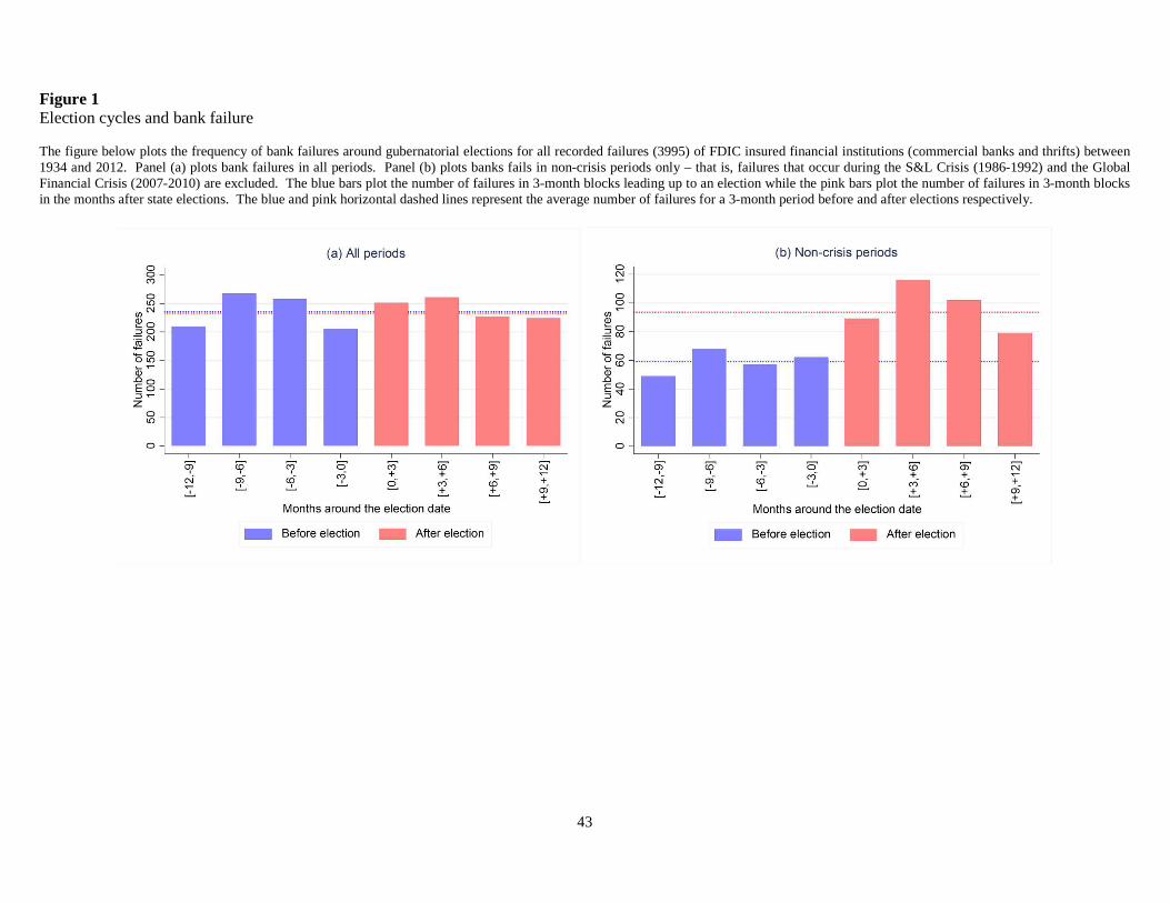
43
Figure 1 Election cycles and bank failure The figure below plots the frequency of bank failures around gubernatorial elections for all recorded failures (3995) of FDIC insured financial institutions (commercial banks and thrifts) between 1934 and 2012. Panel (a) plots bank failures in all periods. Panel (b) plots banks fails in non-crisis periods only – that is, failures that occur during the S&L Crisis (1986-1992) and the Global Financial Crisis (2007-2010) are excluded. The blue bars plot the number of failures in 3-month blocks leading up to an election while the pink bars plot the number of failures in 3-month blocks in the months after state elections. The blue and pink horizontal dashed lines represent the average number of failures for a 3-month period before and after elections respectively.
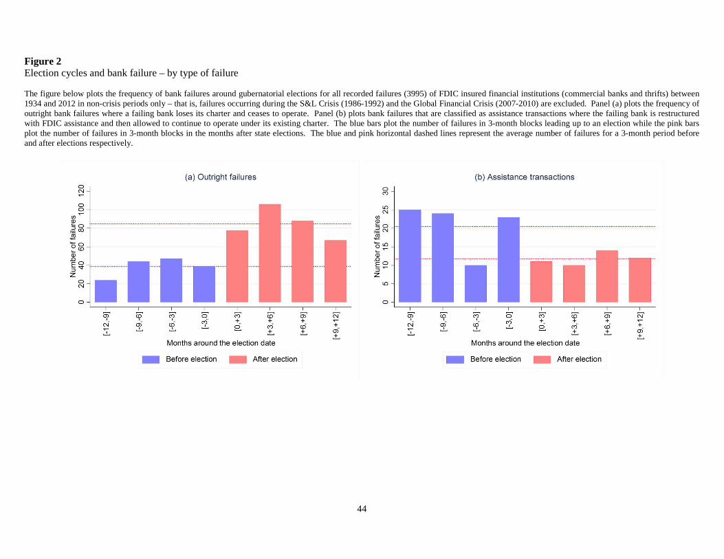
44
Figure 2 Election cycles and bank failure – by type of failure The figure below plots the frequency of bank failures around gubernatorial elections for all recorded failures (3995) of FDIC insured financial institutions (commercial banks and thrifts) between 1934 and 2012 in non-crisis periods only – that is, failures occurring during the S&L Crisis (1986-1992) and the Global Financial Crisis (2007-2010) are excluded. Panel (a) plots the frequency of outright bank failures where a failing bank loses its charter and ceases to operate. Panel (b) plots bank failures that are classified as assistance transactions where the failing bank is restructured with FDIC assistance and then allowed to continue to operate under its existing charter. The blue bars plot the number of failures in 3-month blocks leading up to an election while the pink bars plot the number of failures in 3-month blocks in the months after state elections. The blue and pink horizontal dashed lines represent the average number of failures for a 3-month period before and after elections respectively.
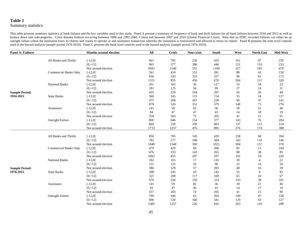
45
Table 1 Summary statistics This table presents summary statistics of bank failures and the key variables used in this study. Panel A present a summary of frequency of bank and thrift failures for all bank failures between 1934 and 2012 as well as broken down into subcategories. Crisis denotes failures occurring between 1986 and 1992 (S&L Crisis) and between 2007 and 2010 (Global Financial Crisis). Note that an FDIC recorded failures can either be an outright failure where the institution loses its charter and ceases to operate or and assistance transaction whereby the institution is restructured and allowed to retain its charter. Panel B presents the state level controls used in the hazard analysis (sample period 1976-2010). Panel C presents the bank level controls used in the hazard analysis (sample period 1976-2010). Panel A: Failures Months around election All Crisis Non-crisis South West North East Mid-West
Sample Period: 1934-2012
All Banks and Thrifts [-12,0] 941 705 236 433 161 97 250
[0,+12] 963 577 386 446 151 133 233
Not around election 2091 1540 551 1100 317 195 479
Commercial Banks Only [-12,0] 561 410 151 281 88 42 150
[0,+12] 656 333 323 327 96 61 172
Not around election 1311 855 456 676 204 111 320
National Banks [-12,0] 201 165 36 127 33 18 23
[0,+12] 181 125 56 99 27 24 31
Not around election 433 329 104 297 56 36 44
State Banks [-12,0] 360 245 115 154 55 24 127
[0,+12] 475 208 267 228 69 37 141
Not around election 878 526 352 379 148 75 276
Assistance [-12,0] 141 59 82 56 18 21 46
[0,+12] 94 47 47 43 14 18 19
Not around election 358 283 75 205 41 21 91
Outright Failure [-12,0] 800 646 154 377 143 76 204
[0,+12] 869 530 339 403 137 115 214
Not around election 1733 1257 476 895 276 174 388
Sample Period: 1976-2012
All Banks and Thrifts [-12,0] 850 705 145 420 158 68 204
[0,+12] 783 577 206 384 143 110 146
Not around election 1840 1540 300 1021 304 137 378
Commercial Banks Only [-12,0] 470 410 60 268 85 13 104
[0,+12] 476 333 143 265 88 38 85
Not around election 1062 855 207 597 191 54 220
National Banks [-12,0] 182 165 17 126 30 4 22
[0,+12] 151 125 26 96 23 14 18
Not around election 386 329 57 283 48 16 39
State Banks [-12,0] 288 245 43 142 55 9 82
[0,+12] 325 208 117 169 65 24 67
Not around election 676 526 150 314 143 38 181
Assistance [-12,0] 141 59 82 56 18 21 46
[0,+12] 93 47 46 43 14 17 19
Not around election 357 283 74 205 41 21 90
Outright Failure [-12,0] 709 646 63 364 140 47 158
[0,+12] 690 530 160 341 129 93 127
Not around election 1483 1257 226 816 263 116 288
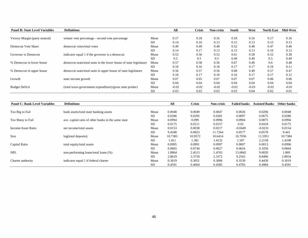
46
Panel B: State Level Variables Definitions All Crisis Non-crisis South West North East Mid-West Victory Margin (party neutral) winner vote percentage - second vote percentage Mean 0.17 0.18 0.16 0.18 0.16 0.17 0.16
SD 0.14 0.16 0.13 0.15 0.13 0.15 0.13
Democrat Vote Share democrat votes/total votes Mean 0.49 0.49 0.48 0.52 0.48 0.47 0.46
SD 0.14 0.17 0.13 0.15 0.13 0.16 0.12
Governor is Democrat indicator equal 1 if the governor is a democrat Mean 0.53 0.56 0.52 0.61 0.58 0.52 0.38
SD 0.5 0.5 0.5 0.49 0.49 0.5 0.49
% Democrat in lower house democrat seats/total seats in the lower house of state legislature Mean 0.57 0.58 0.56 0.67 0.49 0.6 0.48
SD 0.18 0.16 0.18 0.17 0.17 0.16 0.11
% Democrat in upper house democrat seats/total seats in upper house of state legislature Mean 0.56 0.57 0.56 0.68 0.49 0.57 0.47
SD 0.18 0.17 0.18 0.16 0.17 0.17 0.12
Growth state income growth Mean 0.07 0.05 0.07 0.07 0.07 0.06 0.06
SD 0.04 0.04 0.04 0.04 0.04 0.04 0.04
Budget Deficit (total taxes-government expenditure)/gross state product Mean -0.02 -0.02 -0.02 -0.02 -0.03 -0.02 -0.01 SD 0.03 0.03 0.03 0.03 0.04 0.02 0.01
Panel C: Bank Level Variables Definitions All Crisis Non-crisis Failed banks Assisted Banks Other banks Too Big to Fail bank assets/total state banking assets Mean 0.0048 0.0049 0.0047 0.0026 0.0206 0.0048
SD 0.0286 0.0295 0.0281 0.0097 0.0675 0.0286
Too Many to Fail ave. capital ratio of other banks in the same state Mean 0.0994 0.099 0.0996 0.0904 0.0875 0.0994
SD 0.0175 0.0211 0.0157 0.02 0.0418 0.0175
Income/Asset Ratio net income/total assets Mean 0.0153 0.0038 0.0217 -0.0449 -0.0231 0.0154
SD 9.4348 0.0823 11.7264 0.0577 0.0578 9.441
Size log(total deposits) Mean 10.7383 10.9572 10.6414 10.7036 11.5951 10.7384
SD 1.411 1.381 1.4132 1.507 2.2158 1.4108
Capital Ratio total equity/total assets Mean 0.0995 0.0991 0.0997 0.0007 0.0013 0.0996
SD 0.0665 0.0744 0.0627 0.0616 0.1056 0.0664
NPL non-performing loans/total loans (%) Mean 1.8864 2.4513 1.4763 13.6842 9.6820 1.869
SD 2.8619 3.3759 2.3372 9.2565 8.8496 2.8054
Charter authority indicator equal 1 if federal charter Mean 0.3019 0.3051 0.3006 0.3539 0.4430 0.3019 SD 0.4591 0.4604 0.4585 0.4783 0.4984 0.4591
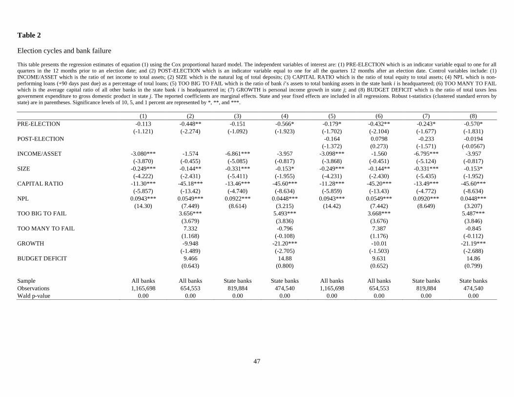
47
Table 2
Election cycles and bank failure This table presents the regression estimates of equation (1) using the Cox proportional hazard model. The independent variables of interest are: (1) PRE-ELECTION which is an indicator variable equal to one for all quarters in the 12 months prior to an election date; and (2) POST-ELECTION which is an indicator variable equal to one for all the quarters 12 months after an election date. Control variables include: (1) INCOME/ASSET which is the ratio of net income to total assets; (2) SIZE which is the natural log of total deposits; (3) CAPITAL RATIO which is the ratio of total equity to total assets; (4) NPL which is non-performing loans (+90 days past due) as a percentage of total loans; (5) TOO BIG TO FAIL which is the ratio of bank i’s assets to total banking assets in the state bank i is headquartered; (6) TOO MANY TO FAIL which is the average capital ratio of all other banks in the state bank i is headquartered in; (7) GROWTH is personal income growth in state j; and (8) BUDGET DEFICIT which is the ratio of total taxes less government expenditure to gross domestic product in state j. The reported coefficients are marginal effects. State and year fixed effects are included in all regressions. Robust t-statistics (clustered standard errors by state) are in parentheses. Significance levels of 10, 5, and 1 percent are represented by *, **, and ***.
(1) (2) (3) (4) (5) (6) (7) (8)
PRE-ELECTION -0.113 -0.448** -0.151 -0.566* -0.179* -0.432** -0.243* -0.570* (-1.121) (-2.274) (-1.092) (-1.923) (-1.702) (-2.104) (-1.677) (-1.831)
POST-ELECTION -0.164 0.0798 -0.233 -0.0194 (-1.372) (0.273) (-1.571) (-0.0567)
INCOME/ASSET -3.080*** -1.574 -6.861*** -3.957 -3.098*** -1.560 -6.795*** -3.957
(-3.870) (-0.455) (-5.085) (-0.817) (-3.868) (-0.451) (-5.124) (-0.817)
SIZE -0.249*** -0.144** -0.331*** -0.153* -0.249*** -0.144** -0.331*** -0.153*
(-4.222) (-2.431) (-5.411) (-1.955) (-4.231) (-2.430) (-5.435) (-1.952)
CAPITAL RATIO -11.30*** -45.18*** -13.46*** -45.60*** -11.28*** -45.20*** -13.49*** -45.60*** (-5.857) (-13.42) (-4.740) (-8.634) (-5.859) (-13.43) (-4.772) (-8.634)
NPL 0.0943*** 0.0549*** 0.0922*** 0.0448*** 0.0943*** 0.0549*** 0.0920*** 0.0448*** (14.30) (7.449) (8.614) (3.215) (14.42) (7.442) (8.649) (3.207)
TOO BIG TO FAIL 3.656*** 5.493*** 3.668*** 5.487***
(3.679)
(3.836)
(3.676)
(3.846)
TOO MANY TO FAIL
7.332
-0.796
7.387
-0.845
(1.168)
(-0.108)
(1.176)
(-0.112)
GROWTH
-9.948
-21.20***
-10.01
-21.19*** (-1.489) (-2.705) (-1.503) (-2.688)
BUDGET DEFICIT 9.466 14.88 9.631 14.86 (0.643) (0.800) (0.652) (0.799)
Sample All banks All banks State banks State banks All banks All banks State banks State banks Observations 1,165,698 654,553 819,884 474,540 1,165,698 654,553 819,884 474,540 Wald p-value 0.00 0.00 0.00 0.00 0.00 0.00 0.00 0.00
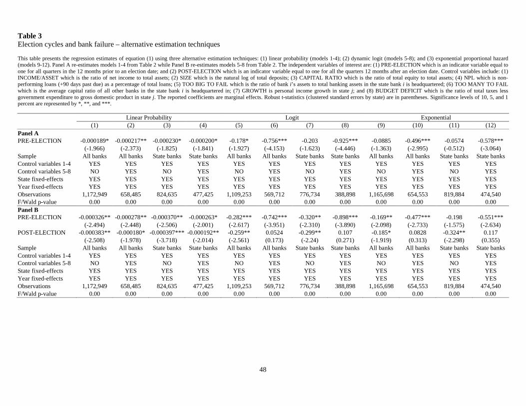
48
Table 3 Election cycles and bank failure – alternative estimation techniques This table presents the regression estimates of equation (1) using three alternative estimation techniques: (1) linear probability (models 1-4); (2) dynamic logit (models 5-8); and (3) exponential proportional hazard (models 9-12). Panel A re-estimates models 1-4 from Table 2 while Panel B re-estimates models 5-8 from Table 2. The independent variables of interest are: (1) PRE-ELECTION which is an indicator variable equal to one for all quarters in the 12 months prior to an election date; and (2) POST-ELECTION which is an indicator variable equal to one for all the quarters 12 months after an election date. Control variables include: (1) INCOME/ASSET which is the ratio of net income to total assets; (2) SIZE which is the natural log of total deposits; (3) CAPITAL RATIO which is the ratio of total equity to total assets; (4) NPL which is non-performing loans (+90 days past due) as a percentage of total loans; (5) TOO BIG TO FAIL which is the ratio of bank i’s assets to total banking assets in the state bank i is headquartered; (6) TOO MANY TO FAIL which is the average capital ratio of all other banks in the state bank i is headquartered in; (7) GROWTH is personal income growth in state j; and (8) BUDGET DEFICIT which is the ratio of total taxes less government expenditure to gross domestic product in state j. The reported coefficients are marginal effects. Robust t-statistics (clustered standard errors by state) are in parentheses. Significance levels of 10, 5, and 1 percent are represented by *, **, and ***. Linear Probability Logit Exponential
(1) (2) (3) (4) (5) (6) (7) (8) (9) (10) (11) (12)
Panel A PRE-ELECTION -0.000189* -0.000217** -0.000230* -0.000200* -0.178* -0.756*** -0.203 -0.925*** -0.0885 -0.496*** -0.0574 -0.578***
(-1.966) (-2.373) (-1.825) (-1.841) (-1.927) (-4.153) (-1.623) (-4.446) (-1.363) (-2.995) (-0.512) (-3.064) Sample All banks All banks State banks State banks All banks All banks State banks State banks All banks All banks State banks State banks Control variables 1-4 YES YES YES YES YES YES YES YES YES YES YES YES Control variables 5-8 NO YES NO YES NO YES NO YES NO YES NO YES State fixed-effects YES YES YES YES YES YES YES YES YES YES YES YES Year fixed-effects YES YES YES YES YES YES YES YES YES YES YES YES Observations 1,172,949 658,485 824,635 477,425 1,109,253 569,712 776,734 388,898 1,165,698 654,553 819,884 474,540 F/Wald p-value 0.00 0.00 0.00 0.00 0.00 0.00 0.00 0.00 0.00 0.00 0.00 0.00 Panel B PRE-ELECTION -0.000326** -0.000278** -0.000370** -0.000263* -0.282*** -0.742*** -0.320** -0.898*** -0.169** -0.477*** -0.198 -0.551***
(-2.494) (-2.448) (-2.506) (-2.001) (-2.617) (-3.951) (-2.310) (-3.890) (-2.098) (-2.733) (-1.575) (-2.634)
POST-ELECTION -0.000383** -0.000180* -0.000397*** -0.000192** -0.259** 0.0524 -0.299** 0.107 -0.185* 0.0828 -0.324** 0.117
(-2.508) (-1.978) (-3.718) (-2.014) (-2.561) (0.173) (-2.24) (0.271) (-1.919) (0.313) (-2.298) (0.355)
Sample All banks All banks State banks State banks All banks All banks State banks State banks All banks All banks State banks State banks Control variables 1-4 YES YES YES YES YES YES YES YES YES YES YES YES Control variables 5-8 NO YES NO YES NO YES NO YES NO YES NO YES State fixed-effects YES YES YES YES YES YES YES YES YES YES YES YES Year fixed-effects YES YES YES YES YES YES YES YES YES YES YES YES Observations 1,172,949 658,485 824,635 477,425 1,109,253 569,712 776,734 388,898 1,165,698 654,553 819,884 474,540 F/Wald p-value 0.00 0.00 0.00 0.00 0.00 0.00 0.00 0.00 0.00 0.00 0.00 0.00
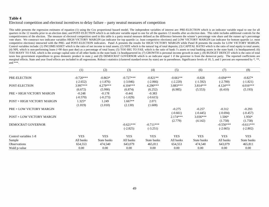
49
Table 4 Electoral competition and electoral incentives to delay failure – party neutral measures of competition This table presents the regression estimates of equation (1) using the Cox proportional hazard model. The independent variables of interest are: PRE-ELECTION which is an indicator variable equal to one for all quarters in the 12 months prior to an election date; and POST-ELECTION which is an indicator variable equal to one for all the quarters 12 months after an election date. This table includes additional controls for the competitiveness of the election. The measure of electoral competition used in this table is a party neutral measure defined as the difference between the winner’s percentage vote share and the runner up’s percentage vote share. We construct two indicator variables HIGH VICTORY MARGIN (an indicator for top quartile i.e. least competitive elections) and LOW VICTORY MARGIN (an indicator for bottom quartile i.e. most competitive elections) interacted with the PRE- and POST-ELECTION indicators. Panel A presents the results for HIGH VICTORY MARGIN while Panel B presents the results for LOW VICTORY MARGIN. Control variables include: (1) INCOME/ASSET which is the ratio of net income to total assets; (2) SIZE which is the natural log of total deposits; (3) CAPITAL RATIO which is the ratio of total equity to total assets; (4) NPL which is non-performing loans (+90 days past due) as a percentage of total loans; (5) TOO BIG TO FAIL which is the ratio of bank i’s assets to total banking assets in the state bank i is headquartered; (6) TOO MANY TO FAIL which is the average capital ratio of all other banks in the state bank i is headquartered in; (7) GROWTH is personal income growth in state j; (8) BUDGET DEFICIT which is the ratio of total taxes less government expenditure to gross domestic product in state j; and (9) DEMOCRAT GOVERNOR which is an indicator equal 1 if the governor is from the democrat party. The reported coefficients are marginal effects. State and year fixed effects are included in all regressions. Robust t-statistics (clustered standard errors by state) are in parentheses. Significance levels of 10, 5, and 1 percent are represented by *, **, and ***. (1) (2) (3) (4) (5) (6) (7) (8)
PRE-ELECTION -0.720*** -0.863* -0.727*** -0.821** -0.661** -0.828 -0.694*** -0.827*
(-2.652) (-1.876) (-3.046) (-2.066) (-2.220) (-1.592) (-2.700) (-1.821)
POST-ELECTION 3.997*** 4.279*** 4.104*** 4.290*** 3.883*** 3.814*** 4.124*** 4.016*** (6.672) (5.990) (6.874) (6.252) (6.985) (5.553) (6.410) (5.193)
PRE × HIGH VICTORY MARGIN -0.248 -0.178 -0.441 -0.383 (-0.570) (-0.273) (-1.029) (-0.615)
POST × HIGH VICTORY MARGIN 1.325* 1.249 1.667** 2.071
(1.819) (1.010) (2.130) (1.608)
PRE × LOW VICTORY MARGIN -0.275 -0.257 -0.312 -0.293 (-0.661) (-0.445) (-0.694) (-0.457) POST × LOW VICTORY MARGIN 2.174*** 3.036*** 1.506* 1.956* (2.779) (4.142) (1.758) (1.758) DEMOCRAT GOVERNOR -0.621*** -0.711*** -0.556*** -0.611*** (-2.825) (-3.251) (-2.665) (-2.802) Control variables 1-8 YES YES YES YES YES YES YES YES Sample All banks State banks All banks State banks All banks State banks All banks State banks Observations 654,553 474,540 643,079 465,811 654,553 474,540 643,079 465,811 Wald p-value 0.00 0.00 0.00 0.00 0.00 0.00 0.00 0.00
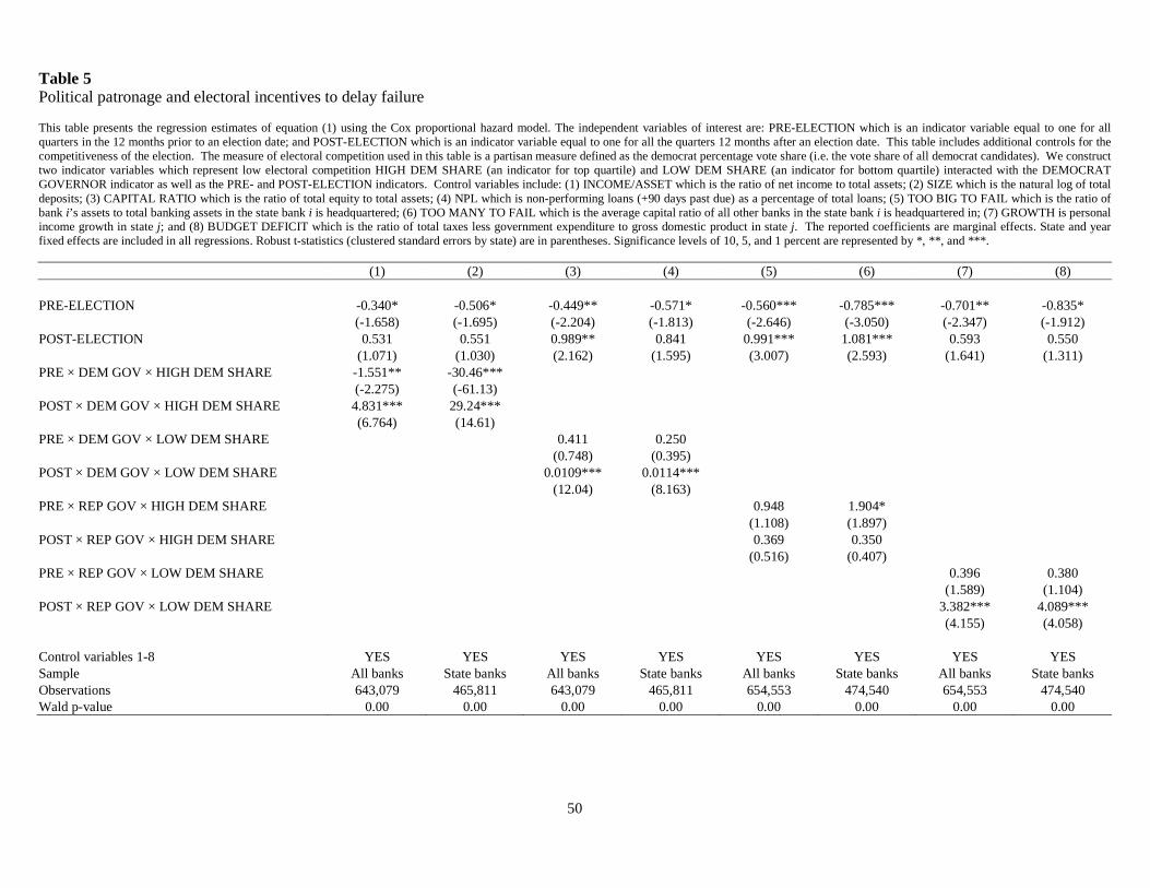
50
Table 5 Political patronage and electoral incentives to delay failure This table presents the regression estimates of equation (1) using the Cox proportional hazard model. The independent variables of interest are: PRE-ELECTION which is an indicator variable equal to one for all quarters in the 12 months prior to an election date; and POST-ELECTION which is an indicator variable equal to one for all the quarters 12 months after an election date. This table includes additional controls for the competitiveness of the election. The measure of electoral competition used in this table is a partisan measure defined as the democrat percentage vote share (i.e. the vote share of all democrat candidates). We construct two indicator variables which represent low electoral competition HIGH DEM SHARE (an indicator for top quartile) and LOW DEM SHARE (an indicator for bottom quartile) interacted with the DEMOCRAT GOVERNOR indicator as well as the PRE- and POST-ELECTION indicators. Control variables include: (1) INCOME/ASSET which is the ratio of net income to total assets; (2) SIZE which is the natural log of total deposits; (3) CAPITAL RATIO which is the ratio of total equity to total assets; (4) NPL which is non-performing loans (+90 days past due) as a percentage of total loans; (5) TOO BIG TO FAIL which is the ratio of bank i’s assets to total banking assets in the state bank i is headquartered; (6) TOO MANY TO FAIL which is the average capital ratio of all other banks in the state bank i is headquartered in; (7) GROWTH is personal income growth in state j; and (8) BUDGET DEFICIT which is the ratio of total taxes less government expenditure to gross domestic product in state j. The reported coefficients are marginal effects. State and year fixed effects are included in all regressions. Robust t-statistics (clustered standard errors by state) are in parentheses. Significance levels of 10, 5, and 1 percent are represented by *, **, and ***. (1) (2) (3) (4) (5) (6) (7) (8)
PRE-ELECTION -0.340* -0.506* -0.449** -0.571* -0.560*** -0.785*** -0.701** -0.835*
(-1.658) (-1.695) (-2.204) (-1.813) (-2.646) (-3.050) (-2.347) (-1.912) POST-ELECTION 0.531 0.551 0.989** 0.841 0.991*** 1.081*** 0.593 0.550
(1.071) (1.030) (2.162) (1.595) (3.007) (2.593) (1.641) (1.311)
PRE × DEM GOV × HIGH DEM SHARE -1.551** -30.46*** (-2.275) (-61.13)
POST × DEM GOV × HIGH DEM SHARE 4.831*** 29.24*** (6.764) (14.61)
PRE × DEM GOV × LOW DEM SHARE 0.411 0.250 (0.748) (0.395)
POST × DEM GOV × LOW DEM SHARE 0.0109*** 0.0114***
(12.04) (8.163)
PRE × REP GOV × HIGH DEM SHARE 0.948 1.904* (1.108) (1.897) POST × REP GOV × HIGH DEM SHARE 0.369 0.350 (0.516) (0.407) PRE × REP GOV × LOW DEM SHARE 0.396 0.380 (1.589) (1.104) POST × REP GOV × LOW DEM SHARE 3.382*** 4.089*** (4.155) (4.058) Control variables 1-8 YES YES YES YES YES YES YES YES Sample All banks State banks All banks State banks All banks State banks All banks State banks Observations 643,079 465,811 643,079 465,811 654,553 474,540 654,553 474,540 Wald p-value 0.00 0.00 0.00 0.00 0.00 0.00 0.00 0.00
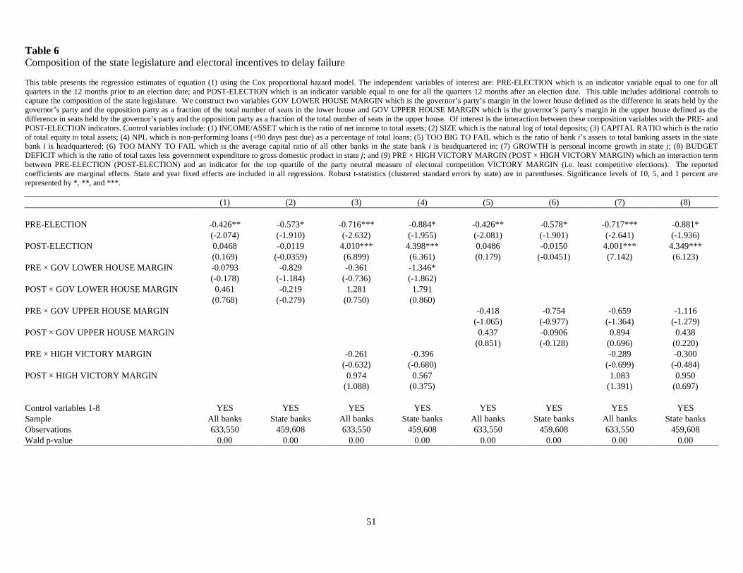
51
Table 6 Composition of the state legislature and electoral incentives to delay failure This table presents the regression estimates of equation (1) using the Cox proportional hazard model. The independent variables of interest are: PRE-ELECTION which is an indicator variable equal to one for all quarters in the 12 months prior to an election date; and POST-ELECTION which is an indicator variable equal to one for all the quarters 12 months after an election date. This table includes additional controls to capture the composition of the state legislature. We construct two variables GOV LOWER HOUSE MARGIN which is the governor’s party’s margin in the lower house defined as the difference in seats held by the governor’s party and the opposition party as a fraction of the total number of seats in the lower house and GOV UPPER HOUSE MARGIN which is the governor’s party’s margin in the upper house defined as the difference in seats held by the governor’s party and the opposition party as a fraction of the total number of seats in the upper house. Of interest is the interaction between these composition variables with the PRE- and POST-ELECTION indicators. Control variables include: (1) INCOME/ASSET which is the ratio of net income to total assets; (2) SIZE which is the natural log of total deposits; (3) CAPITAL RATIO which is the ratio of total equity to total assets; (4) NPL which is non-performing loans (+90 days past due) as a percentage of total loans; (5) TOO BIG TO FAIL which is the ratio of bank i’s assets to total banking assets in the state bank i is headquartered; (6) TOO MANY TO FAIL which is the average capital ratio of all other banks in the state bank i is headquartered in; (7) GROWTH is personal income growth in state j; (8) BUDGET DEFICIT which is the ratio of total taxes less government expenditure to gross domestic product in state j; and (9) PRE × HIGH VICTORY MARGIN (POST × HIGH VICTORY MARGIN) which an interaction term between PRE-ELECTION (POST-ELECTION) and an indicator for the top quartile of the party neutral measure of electoral competition VICTORY MARGIN (i.e. least competitive elections). The reported coefficients are marginal effects. State and year fixed effects are included in all regressions. Robust t-statistics (clustered standard errors by state) are in parentheses. Significance levels of 10, 5, and 1 percent are represented by *, **, and ***. (1) (2) (3) (4) (5) (6) (7) (8)
PRE-ELECTION -0.426** -0.573* -0.716*** -0.884* -0.426** -0.578* -0.717*** -0.881* (-2.074) (-1.910) (-2.632) (-1.955) (-2.081) (-1.901) (-2.641) (-1.936)
POST-ELECTION 0.0468 -0.0119 4.010*** 4.398*** 0.0486 -0.0150 4.001*** 4.349*** (0.169) (-0.0359) (6.899) (6.361) (0.179) (-0.0451) (7.142) (6.123)
PRE × GOV LOWER HOUSE MARGIN -0.0793 -0.829 -0.361 -1.346* (-0.178) (-1.184) (-0.736) (-1.862)
POST × GOV LOWER HOUSE MARGIN 0.461 -0.219 1.281 1.791
(0.768) (-0.279) (0.750) (0.860)
PRE × GOV UPPER HOUSE MARGIN -0.418 -0.754 -0.659 -1.116 (-1.065) (-0.977) (-1.364) (-1.279) POST × GOV UPPER HOUSE MARGIN 0.437 -0.0906 0.894 0.438 (0.851) (-0.128) (0.696) (0.220) PRE × HIGH VICTORY MARGIN -0.261 -0.396 -0.289 -0.300
(-0.632) (-0.680) (-0.699) (-0.484) POST × HIGH VICTORY MARGIN 0.974 0.567 1.083 0.950
(1.088) (0.375) (1.391) (0.697)
Control variables 1-8 YES YES YES YES YES YES YES YES Sample All banks State banks All banks State banks All banks State banks All banks State banks Observations 633,550 459,608 633,550 459,608 633,550 459,608 633,550 459,608 Wald p-value 0.00 0.00 0.00 0.00 0.00 0.00 0.00 0.00
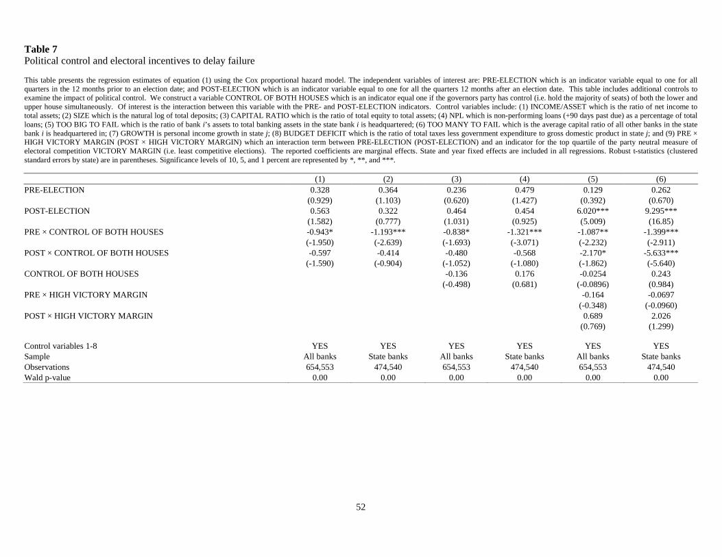
52
Table 7 Political control and electoral incentives to delay failure This table presents the regression estimates of equation (1) using the Cox proportional hazard model. The independent variables of interest are: PRE-ELECTION which is an indicator variable equal to one for all quarters in the 12 months prior to an election date; and POST-ELECTION which is an indicator variable equal to one for all the quarters 12 months after an election date. This table includes additional controls to examine the impact of political control. We construct a variable CONTROL OF BOTH HOUSES which is an indicator equal one if the governors party has control (i.e. hold the majority of seats) of both the lower and upper house simultaneously. Of interest is the interaction between this variable with the PRE- and POST-ELECTION indicators. Control variables include: (1) INCOME/ASSET which is the ratio of net income to total assets; (2) SIZE which is the natural log of total deposits; (3) CAPITAL RATIO which is the ratio of total equity to total assets; (4) NPL which is non-performing loans (+90 days past due) as a percentage of total loans; (5) TOO BIG TO FAIL which is the ratio of bank i’s assets to total banking assets in the state bank i is headquartered; (6) TOO MANY TO FAIL which is the average capital ratio of all other banks in the state bank i is headquartered in; (7) GROWTH is personal income growth in state j; (8) BUDGET DEFICIT which is the ratio of total taxes less government expenditure to gross domestic product in state j; and (9) PRE × HIGH VICTORY MARGIN (POST × HIGH VICTORY MARGIN) which an interaction term between PRE-ELECTION (POST-ELECTION) and an indicator for the top quartile of the party neutral measure of electoral competition VICTORY MARGIN (i.e. least competitive elections). The reported coefficients are marginal effects. State and year fixed effects are included in all regressions. Robust t-statistics (clustered standard errors by state) are in parentheses. Significance levels of 10, 5, and 1 percent are represented by *, **, and ***. (1) (2) (3) (4) (5) (6) PRE-ELECTION 0.328 0.364 0.236 0.479 0.129 0.262
(0.929) (1.103) (0.620) (1.427) (0.392) (0.670)
POST-ELECTION 0.563 0.322 0.464 0.454 6.020*** 9.295***
(1.582) (0.777) (1.031) (0.925) (5.009) (16.85)
PRE × CONTROL OF BOTH HOUSES -0.943* -1.193*** -0.838* -1.321*** -1.087** -1.399*** (-1.950) (-2.639) (-1.693) (-3.071) (-2.232) (-2.911)
POST × CONTROL OF BOTH HOUSES -0.597 -0.414 -0.480 -0.568 -2.170* -5.633*** (-1.590) (-0.904) (-1.052) (-1.080) (-1.862) (-5.640)
CONTROL OF BOTH HOUSES -0.136 0.176 -0.0254 0.243
(-0.498) (0.681) (-0.0896) (0.984)
PRE × HIGH VICTORY MARGIN
-0.164 -0.0697
(-0.348) (-0.0960)
POST × HIGH VICTORY MARGIN
0.689 2.026 (0.769) (1.299)
Control variables 1-8 YES YES YES YES YES YES Sample All banks State banks All banks State banks All banks State banks Observations 654,553 474,540 654,553 474,540 654,553 474,540 Wald p-value 0.00 0.00 0.00 0.00 0.00 0.00
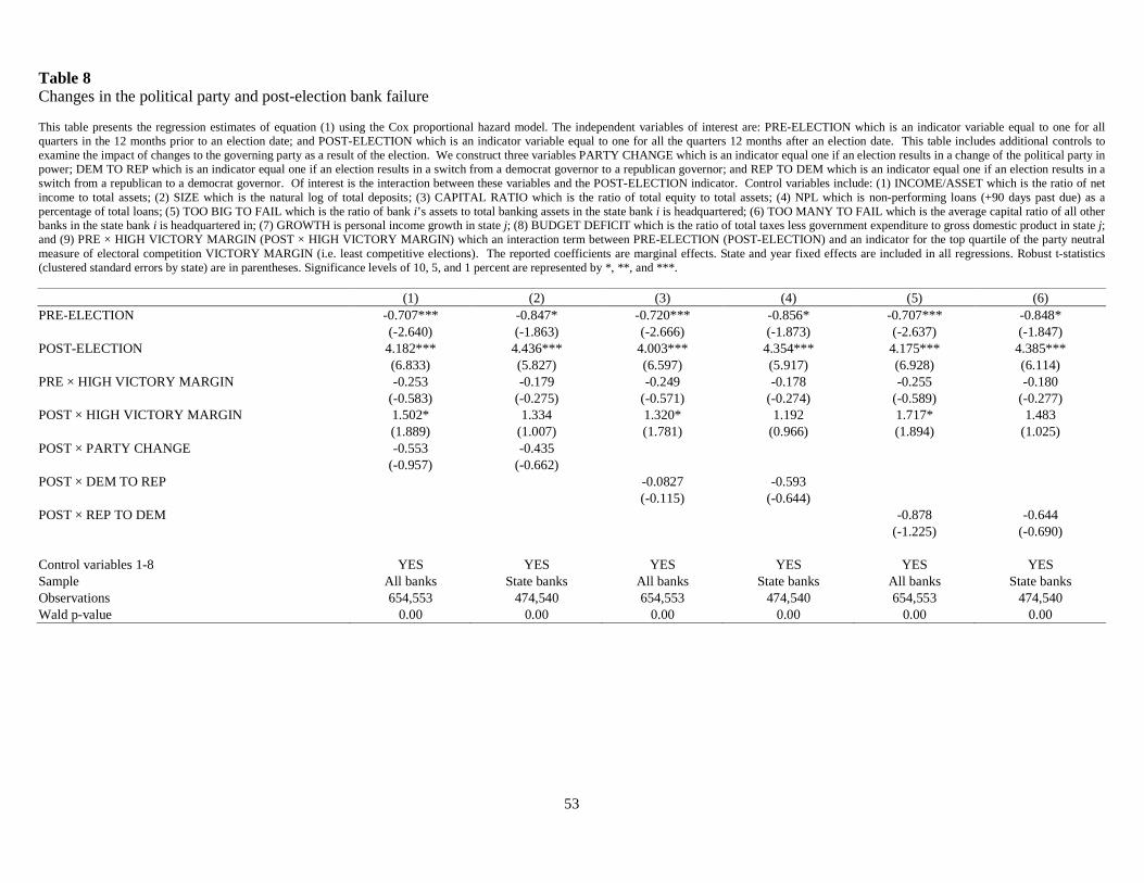
53
Table 8 Changes in the political party and post-election bank failure This table presents the regression estimates of equation (1) using the Cox proportional hazard model. The independent variables of interest are: PRE-ELECTION which is an indicator variable equal to one for all quarters in the 12 months prior to an election date; and POST-ELECTION which is an indicator variable equal to one for all the quarters 12 months after an election date. This table includes additional controls to examine the impact of changes to the governing party as a result of the election. We construct three variables PARTY CHANGE which is an indicator equal one if an election results in a change of the political party in power; DEM TO REP which is an indicator equal one if an election results in a switch from a democrat governor to a republican governor; and REP TO DEM which is an indicator equal one if an election results in a switch from a republican to a democrat governor. Of interest is the interaction between these variables and the POST-ELECTION indicator. Control variables include: (1) INCOME/ASSET which is the ratio of net income to total assets; (2) SIZE which is the natural log of total deposits; (3) CAPITAL RATIO which is the ratio of total equity to total assets; (4) NPL which is non-performing loans (+90 days past due) as a percentage of total loans; (5) TOO BIG TO FAIL which is the ratio of bank i’s assets to total banking assets in the state bank i is headquartered; (6) TOO MANY TO FAIL which is the average capital ratio of all other banks in the state bank i is headquartered in; (7) GROWTH is personal income growth in state j; (8) BUDGET DEFICIT which is the ratio of total taxes less government expenditure to gross domestic product in state j; and (9) PRE × HIGH VICTORY MARGIN (POST × HIGH VICTORY MARGIN) which an interaction term between PRE-ELECTION (POST-ELECTION) and an indicator for the top quartile of the party neutral measure of electoral competition VICTORY MARGIN (i.e. least competitive elections). The reported coefficients are marginal effects. State and year fixed effects are included in all regressions. Robust t-statistics (clustered standard errors by state) are in parentheses. Significance levels of 10, 5, and 1 percent are represented by *, **, and ***. (1) (2) (3) (4) (5) (6) PRE-ELECTION -0.707*** -0.847* -0.720*** -0.856* -0.707*** -0.848*
(-2.640) (-1.863) (-2.666) (-1.873) (-2.637) (-1.847)
POST-ELECTION 4.182*** 4.436*** 4.003*** 4.354*** 4.175*** 4.385* ** (6.833) (5.827) (6.597) (5.917) (6.928) (6.114)
PRE × HIGH VICTORY MARGIN -0.253 -0.179 -0.249 -0.178 -0.255 -0.180 (-0.583) (-0.275) (-0.571) (-0.274) (-0.589) (-0.277)
POST × HIGH VICTORY MARGIN 1.502* 1.334 1.320* 1.192 1.717* 1.483 (1.889) (1.007) (1.781) (0.966) (1.894) (1.025)
POST × PARTY CHANGE -0.553 -0.435
(-0.957) (-0.662)
POST × DEM TO REP
-0.0827 -0.593 (-0.115) (-0.644)
POST × REP TO DEM -0.878 -0.644 (-1.225) (-0.690)
Control variables 1-8 YES YES YES YES YES YES Sample All banks State banks All banks State banks All banks State banks Observations 654,553 474,540 654,553 474,540 654,553 474,540 Wald p-value 0.00 0.00 0.00 0.00 0.00 0.00
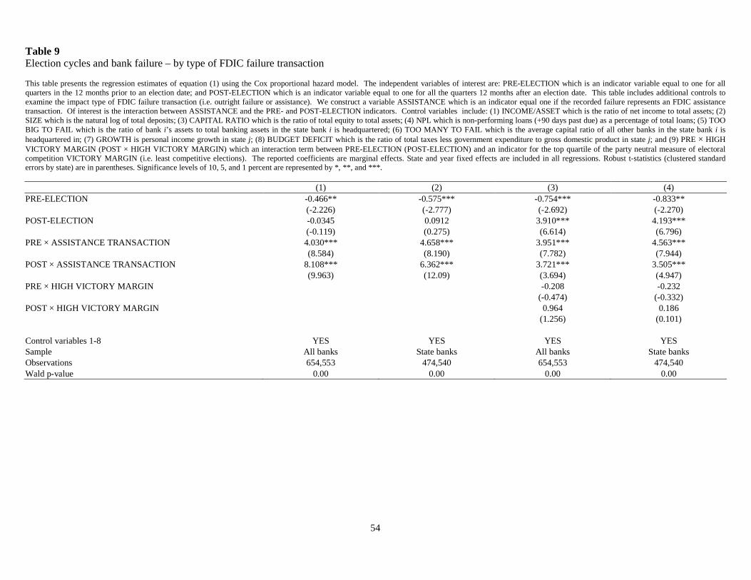
54
Table 9 Election cycles and bank failure – by type of FDIC failure transaction This table presents the regression estimates of equation (1) using the Cox proportional hazard model. The independent variables of interest are: PRE-ELECTION which is an indicator variable equal to one for all quarters in the 12 months prior to an election date; and POST-ELECTION which is an indicator variable equal to one for all the quarters 12 months after an election date. This table includes additional controls to examine the impact type of FDIC failure transaction (i.e. outright failure or assistance). We construct a variable ASSISTANCE which is an indicator equal one if the recorded failure represents an FDIC assistance transaction. Of interest is the interaction between ASSISTANCE and the PRE- and POST-ELECTION indicators. Control variables include: (1) INCOME/ASSET which is the ratio of net income to total assets; (2) SIZE which is the natural log of total deposits; (3) CAPITAL RATIO which is the ratio of total equity to total assets; (4) NPL which is non-performing loans (+90 days past due) as a percentage of total loans; (5) TOO BIG TO FAIL which is the ratio of bank i’s assets to total banking assets in the state bank i is headquartered; (6) TOO MANY TO FAIL which is the average capital ratio of all other banks in the state bank i is headquartered in; (7) GROWTH is personal income growth in state j; (8) BUDGET DEFICIT which is the ratio of total taxes less government expenditure to gross domestic product in state j; and (9) PRE × HIGH VICTORY MARGIN (POST × HIGH VICTORY MARGIN) which an interaction term between PRE-ELECTION (POST-ELECTION) and an indicator for the top quartile of the party neutral measure of electoral competition VICTORY MARGIN (i.e. least competitive elections). The reported coefficients are marginal effects. State and year fixed effects are included in all regressions. Robust t-statistics (clustered standard errors by state) are in parentheses. Significance levels of 10, 5, and 1 percent are represented by *, **, and ***. (1) (2) (3) (4) PRE-ELECTION -0.466** -0.575*** -0.754*** -0.833**
(-2.226) (-2.777) (-2.692) (-2.270) POST-ELECTION -0.0345 0.0912 3.910*** 4.193***
(-0.119) (0.275) (6.614) (6.796) PRE × ASSISTANCE TRANSACTION 4.030*** 4.658*** 3.951*** 4.563*** (8.584) (8.190) (7.782) (7.944) POST × ASSISTANCE TRANSACTION 8.108*** 6.362*** 3.721*** 3.505*** (9.963) (12.09) (3.694) (4.947) PRE × HIGH VICTORY MARGIN -0.208 -0.232
(-0.474) (-0.332) POST × HIGH VICTORY MARGIN 0.964 0.186
(1.256) (0.101) Control variables 1-8 YES YES YES YES Sample All banks State banks All banks State banks Observations 654,553 474,540 654,553 474,540 Wald p-value 0.00 0.00 0.00 0.00
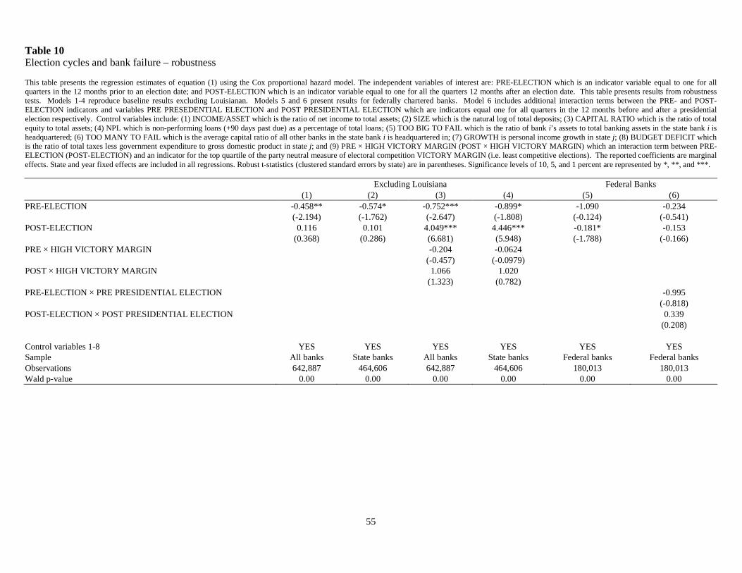
55
Table 10 Election cycles and bank failure – robustness This table presents the regression estimates of equation (1) using the Cox proportional hazard model. The independent variables of interest are: PRE-ELECTION which is an indicator variable equal to one for all quarters in the 12 months prior to an election date; and POST-ELECTION which is an indicator variable equal to one for all the quarters 12 months after an election date. This table presents results from robustness tests. Models 1-4 reproduce baseline results excluding Louisianan. Models 5 and 6 present results for federally chartered banks. Model 6 includes additional interaction terms between the PRE- and POST-ELECTION indicators and variables PRE PRESEDENTIAL ELECTION and POST PRESIDENTIAL ELECTION which are indicators equal one for all quarters in the 12 months before and after a presidential election respectively. Control variables include: (1) INCOME/ASSET which is the ratio of net income to total assets; (2) SIZE which is the natural log of total deposits; (3) CAPITAL RATIO which is the ratio of total equity to total assets; (4) NPL which is non-performing loans (+90 days past due) as a percentage of total loans; (5) TOO BIG TO FAIL which is the ratio of bank i’s assets to total banking assets in the state bank i is headquartered; (6) TOO MANY TO FAIL which is the average capital ratio of all other banks in the state bank i is headquartered in; (7) GROWTH is personal income growth in state j; (8) BUDGET DEFICIT which is the ratio of total taxes less government expenditure to gross domestic product in state j; and (9) PRE × HIGH VICTORY MARGIN (POST × HIGH VICTORY MARGIN) which an interaction term between PRE-ELECTION (POST-ELECTION) and an indicator for the top quartile of the party neutral measure of electoral competition VICTORY MARGIN (i.e. least competitive elections). The reported coefficients are marginal effects. State and year fixed effects are included in all regressions. Robust t-statistics (clustered standard errors by state) are in parentheses. Significance levels of 10, 5, and 1 percent are represented by *, **, and ***. Excluding Louisiana Federal Banks
(1) (2) (3) (4) (5) (6) PRE-ELECTION -0.458** -0.574* -0.752*** -0.899* -1.090 -0.234
(-2.194) (-1.762) (-2.647) (-1.808) (-0.124) (-0.541)
POST-ELECTION 0.116 0.101 4.049*** 4.446*** -0.181* -0.153
(0.368) (0.286) (6.681) (5.948) (-1.788) (-0.166)
PRE × HIGH VICTORY MARGIN -0.204 -0.0624 (-0.457) (-0.0979)
POST × HIGH VICTORY MARGIN 1.066 1.020 (1.323) (0.782)
PRE-ELECTION × PRE PRESIDENTIAL ELECTION
-0.995
(-0.818)
POST-ELECTION × POST PRESIDENTIAL ELECTION
0.339
(0.208)
Control variables 1-8 YES YES YES YES YES YES Sample All banks State banks All banks State banks Federal banks Federal banks Observations 642,887 464,606 642,887 464,606 180,013 180,013 Wald p-value 0.00 0.00 0.00 0.00 0.00 0.00