MPRAMunich Personal RePEc Archive

Union, efficiency of labour andendogenous growth

Chandril Bhattacharyya and Manash Ranjan Gupta

Indian Statistical Institute, Indian Statistical Institute

15. May 2015

Online at http://mpra.ub.uni-muenchen.de/64911/MPRA Paper No. 64911, posted 9. June 2015 15:42 UTC

Union, Efficiency of Labour and Endogenous Growth by

Chandril Bhattacharyya∗ and Manash Ranjan Gupta

15th May, 2015

Abstract: This paper develops an endogenous growth model with human capital formation and

‘Efficiency Wage Hypothesis’ to investigate the growth effect of unionisation and to analyse

properties of optimum income tax rate in the presence of an unionised labour market and with

taxation only on labour income. ‘Efficient Bargaining’ model as well as ‘Right to Manage’

model is used to solve the negotiation problem between the labour union and the employer’s

association. In both type modelling framework, the growth effect of unionisation is

independent of its employment effect; and it depends on its net effect on worker’s efficiency.

The growth rate maximizing tax rate on labour income is different from the corresponding

welfare maximizing tax rate; and the nature of the growth effect of unionisation is different

from its welfare effect.

JEL classification: J51; O41; J31; J24; H52; H21

Keywords: Labour union; Efficiency wage hypothesis; Human capital Formation; income tax;

Endogenous growth

∗ Economic Research Unit, Indian Statistical Institute. Corresponding author: Chandril Bhattacharyya.

1 Introduction:

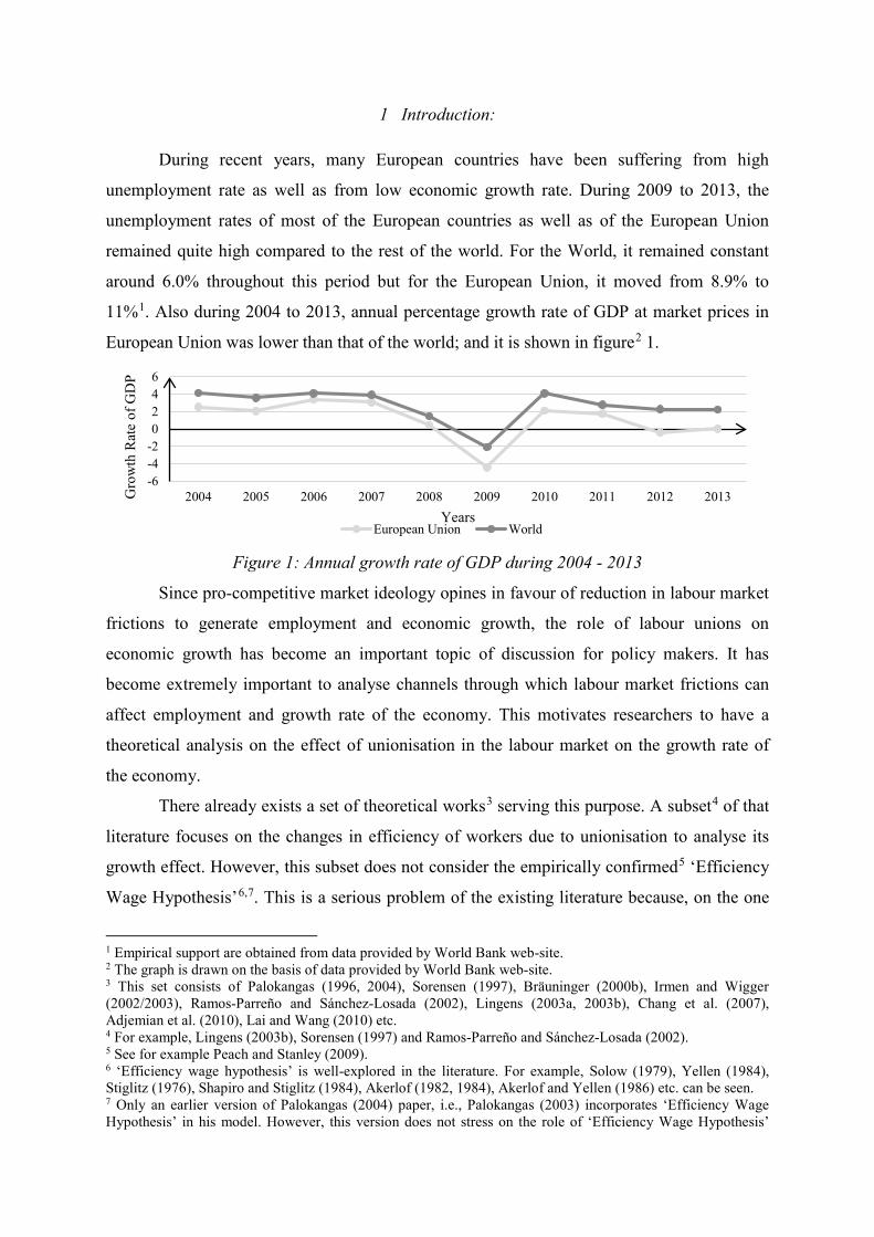
During recent years, many European countries have been suffering from high

unemployment rate as well as from low economic growth rate. During 2009 to 2013, the

unemployment rates of most of the European countries as well as of the European Union

remained quite high compared to the rest of the world. For the World, it remained constant

around 6.0% throughout this period but for the European Union, it moved from 8.9% to

11%1. Also during 2004 to 2013, annual percentage growth rate of GDP at market prices in

European Union was lower than that of the world; and it is shown in figure2 1.

Figure 1: Annual growth rate of GDP during 2004 - 2013

Since pro-competitive market ideology opines in favour of reduction in labour market

frictions to generate employment and economic growth, the role of labour unions on

economic growth has become an important topic of discussion for policy makers. It has

become extremely important to analyse channels through which labour market frictions can

affect employment and growth rate of the economy. This motivates researchers to have a

theoretical analysis on the effect of unionisation in the labour market on the growth rate of

the economy.

There already exists a set of theoretical works3 serving this purpose. A subset4 of that

literature focuses on the changes in efficiency of workers due to unionisation to analyse its

growth effect. However, this subset does not consider the empirically confirmed5 ‘Efficiency

Wage Hypothesis’6,7. This is a serious problem of the existing literature because, on the one

1 Empirical support are obtained from data provided by World Bank web-site. 2 The graph is drawn on the basis of data provided by World Bank web-site. 3 This set consists of Palokangas (1996, 2004), Sorensen (1997), Bräuninger (2000b), Irmen and Wigger (2002/2003), Ramos-Parreño and Sánchez-Losada (2002), Lingens (2003a, 2003b), Chang et al. (2007), Adjemian et al. (2010), Lai and Wang (2010) etc. 4 For example, Lingens (2003b), Sorensen (1997) and Ramos-Parreño and Sánchez-Losada (2002). 5 See for example Peach and Stanley (2009). 6 ‘Efficiency wage hypothesis’ is well-explored in the literature. For example, Solow (1979), Yellen (1984), Stiglitz (1976), Shapiro and Stiglitz (1984), Akerlof (1982, 1984), Akerlof and Yellen (1986) etc. can be seen. 7 Only an earlier version of Palokangas (2004) paper, i.e., Palokangas (2003) incorporates ‘Efficiency Wage Hypothesis’ in his model. However, this version does not stress on the role of ‘Efficiency Wage Hypothesis’

-6-4-20246

2004 2005 2006 2007 2008 2009 2010 2011 2012 2013Gro

wth

Rat

e of

GD

P

YearsEuropean Union World

hand, this hypothesis states that a higher wage rate leads to a higher efficiency level of the

worker8, but, on the other hand, a powerful labour union goes for a higher wage rate. So the

exclusion of ‘Efficiency Wage Hypothesis’ to determine the growth effect of unionisation is a

serious limitation in the model - building literature. Though a few works consider the role of

efficiency wage on union firm bargaining9 using a static framework, they do not analyse its

role on economic growth in a dynamic model.

This subset also ignores the government’s role to raise workers’ efficiency through

investment in human capital accumulation. In most of the countries, the government spends a

huge amount for education to raise the efficiency of workers. The government not only

spends for primary education, secondary education and higher education but also spends for

training of unskilled workers10. The figure 2 presented below11 shows percentages of total

government expenditure allocated for education in a few developed countries for the year

2011.

Figure 2: Expenditure on education as a percentage of total government expenditure

From the figure 2, government’s priority towards skill formation can be easily understood.

The budgeted share of education varies from country to country in between 8% and 16%.

Since the government is a very powerful economic institution and can play an important role

while analysing effects of unionisation. Indeed in a footnote, this fact is accepted and written as “However, the results in this paper hold even if the effort per worker is wholly inflexible……”. However, the published version of this paper, i.e., Palokangas (2004) does not consider the ‘Efficiency Wage Hypothesis’. 8 See sections 9.2 and 9.3 of Romer (2006). 9 Some examples are Garino and Martin (2000), Marti (1997), Mauleon and Vannetelbosch (2003) and Pereau and Sanz (2006). 10 Government also spends for health development of the people to raise their efficiency. However, in this model we overlook the health aspect of workers. As a result, skill level becomes equivalent to the stock of human capital in this model. 11 The graph is drawn on the basis of data provided by World Bank web-site.

02468

1012141618

Perc

enta

ge

Countries

to raise the level of efficiency of workers, we should study the effect of unionisation on

economic growth with a special focus on the government’s role on human capital

accumulation.

There also exists a set12 of theoretical endogenous growth models focusing on human

capital formation and they also do search for optimum taxation. However, these models do

not consider unionised labour markets. In the real world, labour unions are very active in

Europe and in many countries in other continents. The figure 3 gives a concise impression of

this fact showing the labour union density 13 in a few European countries for the year 2012.

Figure 3: Labour union density

Characteristics of unionised labour markets are different from those of competitive labour

markets; and the very presence of labour unions directly affect the mechanism to determine

wage and employment. As a result, the optimum income tax rate imposed to finance human

capital accumulation to raise workers’ efficiency in an unionised labour market should be

different from that obtained in the competitive labour market. So it is very important to

analyse the properties of optimum income tax rate14 to finance investment in human capital

accumulation when the labour market is unionised.

12 This set consists of Blankenau and Simpson (2004), Ni and Wang (1994), Corsetti and Roubini (1996), Glomm and Ravikumar (1997), Chakraborty and Gupta (2009), Bandyopadhyay and Basu (2001), Tournemaine and Tsoukis (Forthcoming) etc. 13 Data for figure 3 are obtained from (http://stats.oecd.org/viewhtml.aspx?datasetcode=UN_DEN&lang=en#). 14 There exists a set of works analysing optimal income tax rate to finance productive public expenditure when labour market is unionised. They are Raurich and Sorolla (2003), Kitaura (2010) etc. However, optimal income tax rate to finance productive public expenditure in an unionised economy should be different from optimal income tax rate to finance investment in human capital accumulation in an unionised economy because the positive externality of productive public capital enjoyed by the private producers is independent of the number of employed workers. Contrary to this, the amount of benefit enjoyed by producers due to rise in the efficiency

0

10

20

30

40

50

60

70

80

90

Labo

ur u

nion

den

sity

Countries

This paper develops a simple endogenous growth model with a special focus on the

‘Efficiency Wage Hypothesis’ and on the government’s role in human capital accumulation.

In this model, we analyse the effect of unionisation on the economic growth rate as well as on

the optimum tax rate to finance public education when the educational expenditure is

financed by taxation only on labour income. Unionisation is defined as an exogenous increase

in the relative bargaining power of the labour union. We use two different bargaining models

to solve the negotiation problem between the employers’ association and the labour union -

‘Efficient Bargaining’ model of McDonald and Solow (1981) and ‘Right to Manage’ model

of Nickell and Andrews (1983).

Our main findings are as follows. First, in each of these two bargaining models, for a

given tax rate on labour income, unionisation lowers the number of employed workers but

raises their effort level. However, when the government imposes the growth rate maximising

tax rate on labour income, then the number of employed workers becomes independent of

labour union’s bargaining power but varies inversely with the elasticity of efficiency with

respect to human capital. Secondly, this growth rate maximising tax rate varies positively

with the elasticity of worker’s efficiency with respect to human capital as well as with the

budget share of investment in human capital accumulation; and, on the other hand, varies

inversely with the degree of unionisation in the labour market. Thirdly, the growth rate

maximising tax rate is different from the corresponding welfare maximising tax rate; and the

welfare effect of unionisation is also different from the growth effect of unionisation in each

of these two bargaining models. Lastly, growth effect of unionisation consists of a positive

effort effect and an ambiguous human capital accumulation effect. In the case of ‘Efficient

Bargaining’ (‘Right to Manage’) model, a higher value of the elasticity of worker’s efficiency

with respect to the wage premium than the value of that elasticity with respect to human

capital is a sufficient but not a necessary (both necessary and sufficient) condition to ensure a

positive growth effect of unionisation. Our results regarding the growth effect of unionisation

is different from those available in the existing literature.

Rest of the paper is organized as follows. In section 2, we describe the basic model

with ‘Efficient Bargaining’. In the section 3, we analyse the existence, uniqueness and

stability of the balanced growth equilibrium. We also analyse properties of growth rate

maximising tax rate and the growth effect of unionisation in this section. In section 4, same

issues are dealt with a ‘Right to Manage’ model. The paper is concluded in the Section 5.

level of workers depends on the number of employed workers which is very much affected by unionisation in the labour market.

2 The model

2.1 Production of final good

The representative competitive firm15 produces the final good, Y, with the following

production function16.

𝑌𝑌 = 𝐴𝐴𝐾𝐾𝛼𝛼(𝑒𝑒𝑒𝑒)𝛽𝛽𝐾𝐾�𝛾𝛾 ; 𝛼𝛼,𝛽𝛽, 𝛾𝛾,𝛼𝛼 + 𝛽𝛽 ∈ (0,1) . (1)

Here A > 0 is a time independent technology parameter and K denotes the amount of capital

used by the representative firm. eL represents firm’s effective employment in efficiency unit

where L stands for the number of workers employed and e stands for the efficiency per

worker.17 𝐾𝐾� symbolizes average quantity of capital stock existing in the economy; and 0 < α

< 1 ensures that the external effect of capital is positive. The Cobb – Douglas production

function satisfies private diminishing returns. However, social returns to scale may not be

diminishing. Decreasing returns to private inputs in the production function results into a

positive profit in equilibrium; and this profit is the rent in the bargaining to be negotiated

between the employers’ association and the labour union. Following Chang et al. (2007), we

assume that fixed amount of land is necessary to setup a firm; and as a result, the number of

firms remains unchanged even in the presence of positive profit.18

We assume that net efficiency per worker, 𝑒𝑒, depends on his accumulated stock of

efficiency, 𝑒𝑒1, as well as on his effort level, 𝑒𝑒2. Efficiency stock of a worker, 𝑒𝑒1, varies

positively with his level of human capital. This is consistent with the assumptions made in

Lucas (1988), Uzawa (1965), Caballé and Santos (1993), Bucci (2008), Docquier et al.

(2008) etc. His effort level, 𝑒𝑒2, varies positively with his net wage relative to his net

reservation income. This keeps consistency with the assumption made by the ‘Efficiency

Wage Hypothesis’.19 For simplicity, we assume that a worker's net reservation income is the

after tax unemployment benefit given to an unemployed worker. So the worker’s net

efficiency, e, is given by 20

15 Following Chang et al. (2007), here also free entry assumption of perfect competition is restricted by the existence of a fixed factor land. Necessity of this assumption will be discussed in a little while. 16 Chang et al. (2007) does not consider efficiency of workers, e. Otherwise, this production function is identical to that in Chang et al. (2007). 17 It is assumed that all workers have identical efficiency level. 18 Number of firms is normalized to unity. 19 See footnotes 6 and 8. 20 Danthine and Kurmann (2006) has also used similar functional form.

𝑒𝑒 = 𝑒𝑒1𝑒𝑒2 . (2)

Here

𝑒𝑒1 = ℎ𝜂𝜂 with 0 < 𝜂𝜂 < 1 ; (2.𝑎𝑎)

and

𝑒𝑒2 = �[1 − 𝜏𝜏]𝑤𝑤[1 − 𝜏𝜏]𝑏𝑏

�𝛿𝛿

= �𝑤𝑤𝑏𝑏�𝛿𝛿

with 0 < 𝛿𝛿 < 1 . (2. 𝑏𝑏)

Here h and w denote the level of human capital and the wage rate respectively; and b stands

for the rate of unemployment benefit. η and 𝛿𝛿 represent elasticities of net efficiency with

respect to the stock of human capital and with respect to the relative wage rate respectively;

and they are assumed to be positive fractions. Chang et al. (2007) does not distinguish

between labour time and labour efficiency. So, in Chang et al. (2007), 𝑒𝑒 ≡ 𝑒𝑒1 ≡ 𝑒𝑒2 ≡ 1, i.e.,

η = δ = 0.

The firm maximises profit, 𝜋𝜋, given by

𝜋𝜋 = 𝑌𝑌 − 𝑤𝑤𝑒𝑒 − 𝑟𝑟𝐾𝐾 (3)

where r represents rental rate on capital.

Capital market is perfectly competitive; and so the equilibrium value of rental rate on

capital is determined by the supply-demand equality in this market. The inverted demand

function for capital is obtained from firm’s profit maximization exercise; and it is given by

𝑟𝑟 = 𝛼𝛼𝐴𝐴𝐾𝐾𝛼𝛼−1(𝑒𝑒𝑒𝑒)𝛽𝛽𝐾𝐾�𝛾𝛾 =𝛼𝛼𝑌𝑌𝐾𝐾

. (4)

2.2 Government

The government finances investment in human capital accumulation (educational

expenditure) as well as benefit given to unemployed workers. To finance these expenditures,

a proportional tax on wage income as well as on unemployment benefit is imposed at the rate

τ ; and the budget remains balanced at each point of time. The total tax revenue is allocated to

these two types of expenditures in an exogenously given proportion.21 For the sake of

21 Since we do not consider any productive role of unemployment benefit in this model, so endogenous determination of this proportion by maximising the economic growth rate is beyond the scope of this model.

simplicity, it is also assumed that the rate of human capital accumulation is proportional to

the educational expenditure of the government. So we have

𝜆𝜆[τ𝑤𝑤𝑒𝑒 + 𝜏𝜏𝑏𝑏(1 − 𝑒𝑒)] = ℎ ; (5)

and

(1 − 𝜆𝜆)[τ𝑤𝑤𝑒𝑒 + 𝜏𝜏𝑏𝑏(1 − 𝑒𝑒)] = 𝑏𝑏(1 − 𝑒𝑒) . (6)

Here (1 − 𝑒𝑒) is the unemployment level and λ is the fraction of revenue allocated to finance

investment in human capital.

We consider taxation only on labour income but not on capital income. This is due to

three reasons. First, both the channels of expenditure provide benefits to workers and not to

capitalists. Secondly, taxation on capital income makes the analysis complicated. Thirdly,

capital income taxation reduces the net marginal productivity of capital and thereby reduces

the rate of growth. A set of works on public economics consisting of Bräuninger (2000a,

2005), Crossley and Low (2011), Landais et al. (2010), Davidson and Woodbury (1997) etc.

also considers taxation only on wage income to finance unemployment benefit scheme.

2.3 Labour union and Efficient Bargaining

In this model, the labour union derives utility from the net wage premium defined as

the difference between the after tax bargained wage rate and the after tax unemployment

benefit rate22 as well as from the number of members of the union. All employed workers are

assumed to be members of the union.23 The utility function of the labour union is defined as

follows.

𝑢𝑢𝑇𝑇 = [(1 − 𝜏𝜏)𝑤𝑤 − (1 − 𝜏𝜏)𝑏𝑏]𝑚𝑚𝑒𝑒𝑛𝑛 = (1 − 𝜏𝜏)𝑚𝑚(𝑤𝑤 − 𝑏𝑏)𝑚𝑚𝑒𝑒𝑛𝑛 with 𝑚𝑚, 𝑛𝑛 > 0 . (7)

Here 𝑢𝑢𝑇𝑇 symbolizes the level of utility of the labour union. Two parameters, m and n

represent elasticities of labour union’s utility with respect to wage premium and with respect

to number of members respectively. If m > (<) (=) n, then the labour union is said to be wage

22 In Irmen and Wigger (2002/2003), Lingens (2003a) and Lai and Wang (2010), the difference between the bargained wage rate and the competitive wage rate is an argument in the labour union’s utility function. Contrary to this, in Adjemian et al. (2010) and Chang et al. (2007), the difference between the after tax bargained wage rate and the net unemployment benefit is an argument in the labour union’s utility function. So, this paper belongs to the second group. 23 This is due to our assumption of a closed shop labour union.

oriented (employment oriented) (neutral). Chang et al. (2007) contains a brief discussion of

these parameters.

We now consider the ‘Efficient Bargaining’ model where both the wage rate and the

number of employed workers are determined mutually by the labour union and the

employer’s association. To obtain these results of bargaining, we maximize the ‘generalised

Nash product’ function given by

𝜓𝜓 = ( 𝑢𝑢𝑇𝑇 − 𝑢𝑢𝑇𝑇����)𝜃𝜃(𝜋𝜋 − 𝜋𝜋�)(1−𝜃𝜃) satisfying 0 < 𝜃𝜃 < 1 . (8)

Here 𝑢𝑢𝑇𝑇���� and 𝜋𝜋� represent the reservation utility level of the labour union and the reservation

profit level of the firm respectively. 𝑢𝑢𝑇𝑇���� and 𝜋𝜋� are assumed to be zero as, bargaining

disagreement stops production and hence employment. 𝜃𝜃 represents the relative bargaining

power of the labour union. Unionisation is defined as an exogenous increase in the value of

𝜃𝜃.

Now, using equations (3), (7) and (8), we obtain

𝜓𝜓 = {(1 − 𝜏𝜏)𝑚𝑚(𝑤𝑤 − 𝑏𝑏)𝑚𝑚𝑒𝑒𝑛𝑛}𝜃𝜃{𝑌𝑌 − 𝑤𝑤𝑒𝑒 − 𝑟𝑟𝐾𝐾}(1−𝜃𝜃) . (9)

Here 𝜓𝜓 is to be maximised with respect to w and 𝑒𝑒. The first order conditions of

maximization are given by

𝜃𝜃𝑚𝑚𝑤𝑤 − 𝑏𝑏

+(1 − 𝜃𝜃)

[𝑌𝑌 − 𝑤𝑤𝑒𝑒 − 𝑟𝑟𝐾𝐾] �𝛽𝛽𝛿𝛿𝑌𝑌𝑤𝑤

− 𝑒𝑒� = 0 ; (10)

and

𝜃𝜃𝑛𝑛𝑒𝑒

+(1 − 𝜃𝜃)

[𝑌𝑌 − 𝑤𝑤𝑒𝑒 − 𝑟𝑟𝐾𝐾] �𝛽𝛽𝑌𝑌𝑒𝑒− 𝑤𝑤� = 0 . (11)

Using equations (4) and (11) we obtain

𝑤𝑤𝑒𝑒𝑌𝑌

=[𝜃𝜃𝑛𝑛(1 − 𝛼𝛼) + 𝛽𝛽(1 − 𝜃𝜃)]

(1 − 𝜃𝜃 + 𝜃𝜃𝑛𝑛) . (11.𝑎𝑎)

Equation (11.a) shows that the labour share of income is time independent and it varies

positively with the relative bargaining power of the union.24 If the labour union has no

24 𝜕𝜕�𝑤𝑤𝑤𝑤𝑌𝑌 �

𝜕𝜕𝜃𝜃= 𝑛𝑛(1−𝛼𝛼−𝛽𝛽)

(1−𝜃𝜃+𝜃𝜃𝑛𝑛)2> 0 .

bargaining power, i.e., if 𝜃𝜃 = 0, then this labour share of income is equal to its competitive

share, i.e. β. However, if the labour union is a monopolist, i.e., if 𝜃𝜃 = 1, then it takes away all

the income left after paying return on capital; and hence the labour share is equal to (1-α).

Using equations (1), (2), (2.a), (2.b), (4), (6), (10) and (11), we obtain25

𝑒𝑒∗ =[1 − (1 − 𝜆𝜆)𝜏𝜏]

[1 − (1 − 𝜆𝜆)𝜏𝜏] + 𝛩𝛩1(1 − 𝜆𝜆)𝜏𝜏 ; (12)

and

𝑤𝑤∗ = 𝑏𝑏𝛩𝛩1 . (13)

where,

𝛩𝛩1 =[𝜃𝜃𝑛𝑛(1 − 𝛼𝛼 − 𝛽𝛽) + 𝛽𝛽(1 − 𝛿𝛿)(1 − 𝜃𝜃 + 𝜃𝜃𝑛𝑛)]

[𝜃𝜃(𝑛𝑛 −𝑚𝑚)(1 − 𝛼𝛼 − 𝛽𝛽) + 𝛽𝛽(1 − 𝛿𝛿)(1− 𝜃𝜃 + 𝜃𝜃𝑛𝑛)] . (14)

𝛩𝛩1 represents the equilibrium value of the negotiated wage rate relative to the unemployment

benefit rate. We assume the denominator of 𝛩𝛩1 to be positive in order to ensure 0 < 𝑒𝑒∗ < 1.

When the labour union is neutral or employment oriented, i.e., when m ≤ n, the denominator

of 𝛩𝛩1 is always positive. However, when the union is wage oriented, i.e., when m > n, 𝛩𝛩1 > 0

implies that the labour union can not be highly biased for wage premium. This assumption

also implies that 𝛩𝛩1 > 1,26 which further implies that 𝑤𝑤∗ > 𝑏𝑏. Now from equations (2.b) and

(13), we obtain the effort level per worker as given by

𝑒𝑒2∗ = (𝛩𝛩1)𝛿𝛿 . (15)

Equation (12) shows that 𝑒𝑒∗ varies inversely with 𝛩𝛩1. As 𝛩𝛩1 is increased, the union

claims for a higher wage; and so the number of employed workers is reduced. Equation (12)

also shows that 𝑒𝑒∗ → 1 as (1 − 𝜆𝜆) → 0. This implies that unemployment does not exist when

there is no unemployment benefit. The number of employed workers, 𝑒𝑒∗, varies inversely

with (1 − 𝜆𝜆) as well as with 𝜏𝜏. It can be easily shown that

𝜕𝜕𝑒𝑒∗

𝜕𝜕𝜏𝜏= −

(1 − 𝜆𝜆)𝛩𝛩1{[1 − (1 − 𝜆𝜆)𝜏𝜏] + 𝛩𝛩1(1 − 𝜆𝜆)𝜏𝜏}2 < 0 ; (16)

25 See appendix A for derivation of optimal w and L. 26 If the denominator of 𝛩𝛩1 is positive, then 𝛩𝛩1 is greater than unity as the numerator of 𝛩𝛩1 is obviously greater than the denominator of 𝛩𝛩1.

and

𝜕𝜕𝑒𝑒∗

𝜕𝜕𝜆𝜆=

𝜏𝜏𝛩𝛩1{[1 − (1 − 𝜆𝜆)𝜏𝜏] + 𝛩𝛩1(1− 𝜆𝜆)𝜏𝜏}2 > 0 . (17)

As the tax rate is increased and the proportion for funding unemployment benefit remains

unchanged, unemployment benefit per worker, b, is also increased. This unemployment

benefit is the reservation income of the worker. So the labour union wants a higher wage rate

and the employer lowers the number of employed workers in this case. By the similar logic,

the number of employed workers is reduced when the proportion for funding unemployment

benefit is increased but the tax rate remains unchanged.

Now from equation (14), we obtain

𝜕𝜕𝛩𝛩1𝜕𝜕𝜃𝜃

=𝑚𝑚𝛽𝛽(1 − 𝛼𝛼 − 𝛽𝛽)(1 − 𝛿𝛿)

[𝜃𝜃(𝑛𝑛 −𝑚𝑚)(1− 𝛼𝛼 − 𝛽𝛽) + 𝛽𝛽(1 − 𝛿𝛿)(1− 𝜃𝜃 + 𝜃𝜃𝑛𝑛)]2 > 0 ; (18)

and from equation (15), we have

𝜕𝜕𝑒𝑒2∗

𝜕𝜕𝜃𝜃= 𝛿𝛿(𝛩𝛩1)𝛿𝛿−1

𝜕𝜕𝛩𝛩1𝜕𝜕𝜃𝜃

> 0 . (19)

As the labour union becomes more powerful, it claims a higher wage relative to the

alternative income of the worker. As a result of this, equation (19) implies that the effort level

per worker varies positively with the degree of unionisation.

Now, from equations (12) and (18), we obtain

𝜕𝜕𝑒𝑒∗

𝜕𝜕𝜃𝜃= −

[1 − (1 − 𝜆𝜆)𝜏𝜏](1 − 𝜆𝜆)𝜏𝜏{[1 − (1 − 𝜆𝜆)𝜏𝜏] + 𝛩𝛩1(1 − 𝜆𝜆)𝜏𝜏}2

𝜕𝜕𝛩𝛩1𝜕𝜕𝜃𝜃

< 0 . (20)

Equation (20) shows that, given the tax rate, the negotiated number of employed workers

varies inversely with the degree of unionisation. This is so because unionisation raises the

negotiated wage rate as well as the ratio of that wage to the unemployment benefit; and, as a

result, effort level per worker is increased27. This rise in the wage rate reduces the demand for

labour and the rise in worker’s effort level substitutes the number of employed workers. As a

result, number of employed workers declines due to unionisation. We summarize this result

in the following proposition.

27 See equation (19).

Proposition 1: For a given tax rate, unionisation lowers the number of employed workers but

raises the wage rate as well as the effort level of the worker irrespective of the orientation of

the labour union.

Lingens (2003a, 2003b) and Adjemian et al. (2010) consider a neutral labour union

and show that unionisation reduces the number of employed workers due to rise in the wage

rate. On the contrary, Chang et al. (2007) shows that unionisation does not necessarily lower

the number of employed workers; and the employment effect of unionisation is positive for

an employment oriented labour union. However, we consider ‘Efficiency wage hypothesis’

and show that unionisation leads to a decline in the number of employed workers irrespective

of the orientation of the labour union. Our result is due to the substitution effect resulting

from an increase in the efficiency of the worker.

2.4 The representative household

The representative household derives instantaneous utility only from consumption of

the final good28. She maximises her discounted present value of instantaneous utility over the

infinite time horizon subject to her intertemporal budget constraint. So her dynamic

optimisation problem is defined as follows.

𝑀𝑀𝑎𝑎𝑀𝑀�𝑐𝑐1−𝜎𝜎 − 1

1 − 𝜎𝜎𝑒𝑒−𝜌𝜌𝜌𝜌

∞

0

𝑑𝑑𝑑𝑑 (21)

subject to, ��𝐾 = (1 − 𝜏𝜏)𝑤𝑤𝑒𝑒 + 𝑟𝑟𝐾𝐾 + 𝜋𝜋 + (1 − 𝜏𝜏)𝑏𝑏(1 − 𝑒𝑒) − 𝑐𝑐 ; (22)

𝐾𝐾(0) = 𝐾𝐾0 (𝐾𝐾0 is historically given) ;

and 𝑐𝑐 ∈ [0, (1 − 𝜏𝜏)𝑤𝑤𝑒𝑒 + 𝑟𝑟𝐾𝐾 + 𝜋𝜋 + (1 − 𝜏𝜏)𝑏𝑏(1 − 𝑒𝑒)] .

Here c is the consumption level of the representative household; and 𝜎𝜎 and ρ are two

parameters representing elasticity of marginal utility of consumption and the rate of discount

respectively. We assume entire savings to be invested and rule out depreciation of capital. We

also assume that unemployment rate is equal among households. Here c is the control

variable and K is the state variable.

28 For technical simplicity, we assume that the representative household does not obtain utility from her human capital stock. In reality, people enjoy good health as well as respect from others due to his/her skill level.

Solving this dynamic optimisation problem, we derive the rate of growth of

consumption as given by29

𝑔𝑔 =��𝑐𝑐𝑐

=𝛼𝛼𝐴𝐴𝐾𝐾𝛼𝛼−1(𝑒𝑒𝑒𝑒)𝛽𝛽𝐾𝐾�𝛾𝛾 − 𝜌𝜌

𝜎𝜎 . (23)

3 Steady state equilibrium

3.1 Existence and stability

The symmetric steady state growth equilibrium satisfies following properties:

(i) 𝑐𝑐𝑐𝑐=𝐾𝐾𝐾𝐾

=ℎℎ=𝑌𝑌𝑌𝑌

=𝑤𝑤∗

𝑤𝑤∗

=𝜋𝜋𝜋𝜋=��𝑏𝑏𝑏

= 𝑔𝑔 ;

(ii) 𝐾𝐾 = 𝐾𝐾�; and

(iii) r, 𝑒𝑒∗, τ, 𝜆𝜆, 𝑒𝑒2∗ and g are time independent. To ensure that h, K and Y grow at the same

rate, i.e., to satisfy property (i), we further assume that 𝛾𝛾 = 1 − 𝛼𝛼 − 𝛽𝛽𝜂𝜂. This implies that the

production function satisfies the property of social constant returns to scale.

Using equations (1), (2), (2.a), (5), (6), (11.a), (15), (22), (23), and putting 𝛾𝛾 =

1 − 𝛼𝛼 − 𝛽𝛽𝜂𝜂, 𝑒𝑒 = 𝑒𝑒∗ and 𝐾𝐾 = 𝐾𝐾�, we obtain

𝑔𝑔 =��𝑐𝑐𝑐

=𝛼𝛼𝐴𝐴𝑒𝑒∗𝛽𝛽 �ℎ

𝐾𝐾�𝛽𝛽𝜂𝜂

[𝛩𝛩1]𝛽𝛽𝛿𝛿 − 𝜌𝜌𝜎𝜎

; (24)

𝑔𝑔 =ℎℎ

=𝜆𝜆𝜏𝜏[𝜃𝜃𝑛𝑛(1 − 𝛼𝛼) + 𝛽𝛽(1 − 𝜃𝜃)]𝐴𝐴 �𝐾𝐾

ℎ�1−𝛽𝛽𝜂𝜂

𝑒𝑒∗𝛽𝛽[𝛩𝛩1]𝛽𝛽𝛿𝛿

[1 − (1 − 𝜆𝜆)𝜏𝜏](1 − 𝜃𝜃 + 𝜃𝜃𝑛𝑛) ; (25)

and

𝑔𝑔 =��𝐾𝐾𝐾

= 𝐴𝐴𝑒𝑒∗ 𝛽𝛽 �ℎ𝐾𝐾�𝛽𝛽𝜂𝜂

[𝛩𝛩1]𝛽𝛽𝛿𝛿 �1 −𝜆𝜆𝜏𝜏[𝜃𝜃𝑛𝑛(1 − 𝛼𝛼) + 𝛽𝛽(1 − 𝜃𝜃)]

(1 − 𝜃𝜃 + 𝜃𝜃𝑛𝑛)[1 − (1 − 𝜆𝜆)𝜏𝜏]� −𝑐𝑐𝐾𝐾

. (26)

We define two new variables M and N such that M = (c/K) and N = (h/K). So using equations

(24), (25) and (26), we obtain

𝑀𝑀𝑀𝑀

=𝛼𝛼𝐴𝐴𝑒𝑒∗𝛽𝛽(𝑁𝑁)𝛽𝛽𝜂𝜂[𝛩𝛩1]𝛽𝛽𝛿𝛿 − 𝜌𝜌

𝜎𝜎

−𝐴𝐴𝑒𝑒∗ 𝛽𝛽(𝑁𝑁)𝛽𝛽𝜂𝜂[𝛩𝛩1]𝛽𝛽𝛿𝛿 �1 −𝜆𝜆𝜏𝜏[𝜃𝜃𝑛𝑛(1 − 𝛼𝛼) + 𝛽𝛽(1 − 𝜃𝜃)]

(1 − 𝜃𝜃 + 𝜃𝜃𝑛𝑛)[1 − (1 − 𝜆𝜆)𝜏𝜏]� + 𝑀𝑀 ; (27)

and

𝑁𝑁𝑁𝑁

=𝜆𝜆𝜏𝜏[𝜃𝜃𝑛𝑛(1 − 𝛼𝛼) + 𝛽𝛽(1 − 𝜃𝜃)]𝐴𝐴(𝑁𝑁)𝛽𝛽𝜂𝜂−1𝑒𝑒∗𝛽𝛽[𝛩𝛩1]𝛽𝛽𝛿𝛿

[1 − (1 − 𝜆𝜆)𝜏𝜏](1 − 𝜃𝜃 + 𝜃𝜃𝑛𝑛)

29 See appendix B for derivation of equation (23).

−𝐴𝐴𝑒𝑒∗ 𝛽𝛽(𝑁𝑁)𝛽𝛽𝜂𝜂[𝛩𝛩1]𝛽𝛽𝛿𝛿 �1 −𝜆𝜆𝜏𝜏[𝜃𝜃𝑛𝑛(1 − 𝛼𝛼) + 𝛽𝛽(1 − 𝜃𝜃)]

(1 − 𝜃𝜃 + 𝜃𝜃𝑛𝑛)[1 − (1 − 𝜆𝜆)𝜏𝜏]� + 𝑀𝑀 . (28)

In the steady state growth equilibrium, 𝑀𝑀𝑀𝑀 = 𝑁𝑁

𝑁𝑁 = 0; and this implies that

𝛼𝛼𝐴𝐴𝑒𝑒∗𝛽𝛽(𝑁𝑁)𝛽𝛽𝜂𝜂[𝛩𝛩1]𝛽𝛽𝛿𝛿 − 𝜌𝜌

𝜎𝜎=𝜆𝜆𝜏𝜏[𝜃𝜃𝑛𝑛(1 − 𝛼𝛼) + 𝛽𝛽(1 − 𝜃𝜃)]𝐴𝐴(𝑁𝑁)𝛽𝛽𝜂𝜂−1𝑒𝑒∗𝛽𝛽[𝛩𝛩1]𝛽𝛽𝛿𝛿

[1 − (1 − 𝜆𝜆)𝜏𝜏](1 − 𝜃𝜃 + 𝜃𝜃𝑛𝑛) . (29)

Equation (29) is solely a function of N. We now turn to show the existence and uniqueness of

the steady state equilibrium; i.e., a unique solution of equation (29). For this purpose, we use

a diagram. In figure 4, L.H.S. and R.H.S. of equation (29) are measured on the vertical axis

and N on the horizontal axis.

L.H.S.

R.H.S. R.H.S.

L.H.S.

0 𝑁𝑁∗ N

−𝜌𝜌𝜎𝜎

Figure 4: Existence of a unique steady state equilibrium

The L.H.S. curve is positively sloped and is concave to the horizontal axis with a point of

intersection on that axis. However the R.H.S. curve is negatively sloped, convex to the origin

and asymptotic to both axes. The unique point of intersection of these two curves at 𝑁𝑁∗

shows the existence of a unique steady state growth equilibrium.

To analyse stability of the system, we use equations (27) and (28). The mathematical

sign of the Jacobian determinant, given by

|𝐽𝐽| =��𝜕𝜕 �𝑀𝑀

𝑀𝑀 �

𝜕𝜕𝑀𝑀

𝜕𝜕 �𝑀𝑀𝑀𝑀 �

𝜕𝜕𝑁𝑁𝜕𝜕 �𝑁𝑁

𝑁𝑁 �

𝜕𝜕𝑀𝑀𝜕𝜕 �𝑁𝑁

𝑁𝑁�

𝜕𝜕𝑁𝑁

�� ,

is to be evaluated. It can be easily shown that30

|𝐽𝐽| = −�(1 − 𝛽𝛽𝜂𝜂)𝜆𝜆𝜏𝜏[𝜃𝜃𝑛𝑛(1 − 𝛼𝛼) + 𝛽𝛽(1 − 𝜃𝜃)]𝐴𝐴(𝑁𝑁)𝛽𝛽𝜂𝜂−2𝑒𝑒∗𝛽𝛽[𝛩𝛩1]𝛽𝛽𝛿𝛿

[1 − (1 − 𝜆𝜆)𝜏𝜏](1 − 𝜃𝜃 + 𝜃𝜃𝑛𝑛)

+𝛽𝛽𝜂𝜂𝛼𝛼𝐴𝐴𝑒𝑒∗𝛽𝛽(𝑁𝑁)𝛽𝛽𝜂𝜂−1[𝛩𝛩1]𝛽𝛽𝛿𝛿

𝜎𝜎� < 0 ; (30)

And the negative sign of |𝐽𝐽| implies that the two latent roots of J matrix are of opposite sign.

This implies that the unique steady state growth equilibrium is saddle point stable.

3.2 Growth rate maximising tax rate

We assume that the government wants to maximise the rate of growth in the steady state

equilibrium31; and now turn to analyse properties of growth rate maximising tax rate.

Substituting (h/K) from equation (25) into equation (24), we obtain

(𝜌𝜌 + 𝜎𝜎𝑔𝑔)[𝑔𝑔]𝛽𝛽𝛽𝛽

1−𝛽𝛽𝛽𝛽 = 𝐴𝐴1

1−𝛽𝛽𝛽𝛽𝛼𝛼𝑒𝑒∗𝛽𝛽

1−𝛽𝛽𝛽𝛽[𝛩𝛩1]𝛽𝛽𝛽𝛽

1−𝛽𝛽𝛽𝛽 �𝜆𝜆𝜏𝜏[𝜃𝜃𝑛𝑛(1 − 𝛼𝛼) + 𝛽𝛽(1 − 𝜃𝜃)]

[1 − (1 − 𝜆𝜆)𝜏𝜏](1− 𝜃𝜃 + 𝜃𝜃𝑛𝑛)�

𝛽𝛽𝛽𝛽1−𝛽𝛽𝛽𝛽

. (31)

The L.H.S. of equation (31) is a monotonically increasing function of g. So the tax rate,

which maximises the R.H.S. of equation (31), also maximises the growth rate. So from

equations (12) and (31), we obtain the growth rate maximising tax rate as given by

𝜏𝜏∗ =𝜂𝜂

[(1 − 𝜂𝜂)𝛩𝛩1 + 𝜂𝜂](1 − 𝜆𝜆) . (32)

Equation (32) shows that 𝜏𝜏∗32 varies positively with 𝜂𝜂 and 𝜆𝜆. If human capital is not

productive, i.e., if 𝜂𝜂 = 0, then no tax should be imposed in order to maximise the growth rate.

Equation (31) clearly shows that the rate of growth varies inversely with the tax rate when

𝜂𝜂 = 0. This is so because 𝑒𝑒∗ varies inversely with τ. Again, from equation (32), we obtain

𝜕𝜕𝜏𝜏∗

𝜕𝜕𝜃𝜃= −

𝜂𝜂(1 − 𝜂𝜂)[(1 − 𝜂𝜂)𝛩𝛩1 + 𝜂𝜂]2(1 − 𝜆𝜆)

𝜕𝜕𝛩𝛩1𝜕𝜕𝜃𝜃

< 0 . (33)

Equation (33) shows that growth rate maximising tax rate varies inversely with the degree of

unionisation in the labour market. The intuition behind this result is as follows. The change in

tax rate has two opposite effects on the growth rate. The first effect works by reducing

30 See appendix C for derivation of equation (30). 31 Usually it is assumed that the objective of the government is to maximise social welfare. However, for technical simplicity, here we consider growth rate maximization. Agénor and Neanidis (2014) also focuses on growth rate maximisation rather than on welfare maximisation on the ground that, in practice, imperfect knowledge about household preferences makes it easier to measure their income level rather than their welfare level. 32 We assume that the second order condition is satisfied.

employment level and the second effect works by increasing human capital accumulation.

These two effects balances each other at 𝜏𝜏 = 𝜏𝜏∗. Now, a rise in 𝜃𝜃 lowers employment level;

and to raise it back to its previous level, 𝜏𝜏∗ should decline due to the inverse relationship

between 𝑒𝑒∗ and τ. So the growth rate maximising tax rate is reduced due to unionisation in

this case. These properties of growth rate maximising tax rate is summarised in the following

proposition.

Proposition 2: The growth rate maximising tax rate on labour income, on the one hand,

varies positively with the elasticity of efficiency with respect to human capital as well as with

the budget share of investment in human capital accumulation; and, on the other hand, varies

inversely with the degree of unionisation in the labour market.

Incorporating the value of 𝜏𝜏∗ from equation (32) in equation (12), we obtain

𝑒𝑒∗ = 1 − 𝜂𝜂 . (34)

Equation (34) shows that the rate of employment of workers is independent of the degree of

unionisation when government imposes the growth rate maximising tax rate; and it varies

inversely with the elasticity of efficiency with respect to human capital stock. This is so

because unionisation has two different effects on employment. One is the direct effect; and

the other is the indirect effect operating through the change in the tax rate. Equations (20) and

(33) show that both 𝑒𝑒∗ and 𝜏𝜏∗ vary in the same direction with unionisation; and equation (16)

shows that 𝑒𝑒∗ varies inversely with 𝜏𝜏∗. As a result, these two effects of unionisation on 𝑒𝑒∗

cancel out each other; and thus employment level becomes independent of the degree of

unionisation. 𝑒𝑒∗ varies inversely with 𝜂𝜂 because a higher value of 𝜂𝜂 indicates a higher level of

efficiency and the efficiency gain always substitutes the number of employed workers. This is

stated in the following proposition.

Proposition 3: When the government imposes the growth rate maximising tax rate on labour

income, rate of employment becomes independent of the degree of unionisation in the labour

market but varies inversely with the elasticity of efficiency with respect to human capital.

The welfare level of the representative household, ω, is defined as her discounted

present value of instantaneous utility over the infinite time horizon. It is obtained from

equations (1), (3), (6), (11.a), (21), (22) and (23) and is given by33

33 See appendix D for derivation of equation (35).

𝜔𝜔 =𝐾𝐾01−𝜎𝜎 ��

𝜌𝜌+𝜎𝜎𝜎𝜎𝛼𝛼� �1 − 𝜆𝜆τ

[1−(1−𝜆𝜆)τ][𝜃𝜃𝑛𝑛(1−𝛼𝛼)+𝛽𝛽(1−𝜃𝜃)]

(1−𝜃𝜃+𝜃𝜃𝑛𝑛) � − 𝑔𝑔�1−𝜎𝜎

(1 − 𝜎𝜎)[𝜌𝜌 − 𝑔𝑔(1 − 𝜎𝜎)] + 𝑐𝑐𝑐𝑐𝑛𝑛𝑐𝑐𝑑𝑑𝑎𝑎𝑛𝑛𝑑𝑑 . (35)

We assume 1 > σ and ρ > g(1-σ). Since initial consumption 𝑐𝑐0 is positive, so �𝜌𝜌+𝜎𝜎𝜎𝜎𝛼𝛼� �1 −

𝜆𝜆τ[1−(1−𝜆𝜆)τ]

[𝜃𝜃𝑛𝑛(1−𝛼𝛼)+𝛽𝛽(1−𝜃𝜃)](1−𝜃𝜃+𝜃𝜃𝑛𝑛) � has to be greater than g. Here, we do not attempt to derive the

welfare maximising income tax rate on labour income for technical complexity. Rather, here

we check whether the growth rate maximising income tax rate on labour income, given by

equation (32), is identical to the welfare maximising labour income tax rate or not. For this

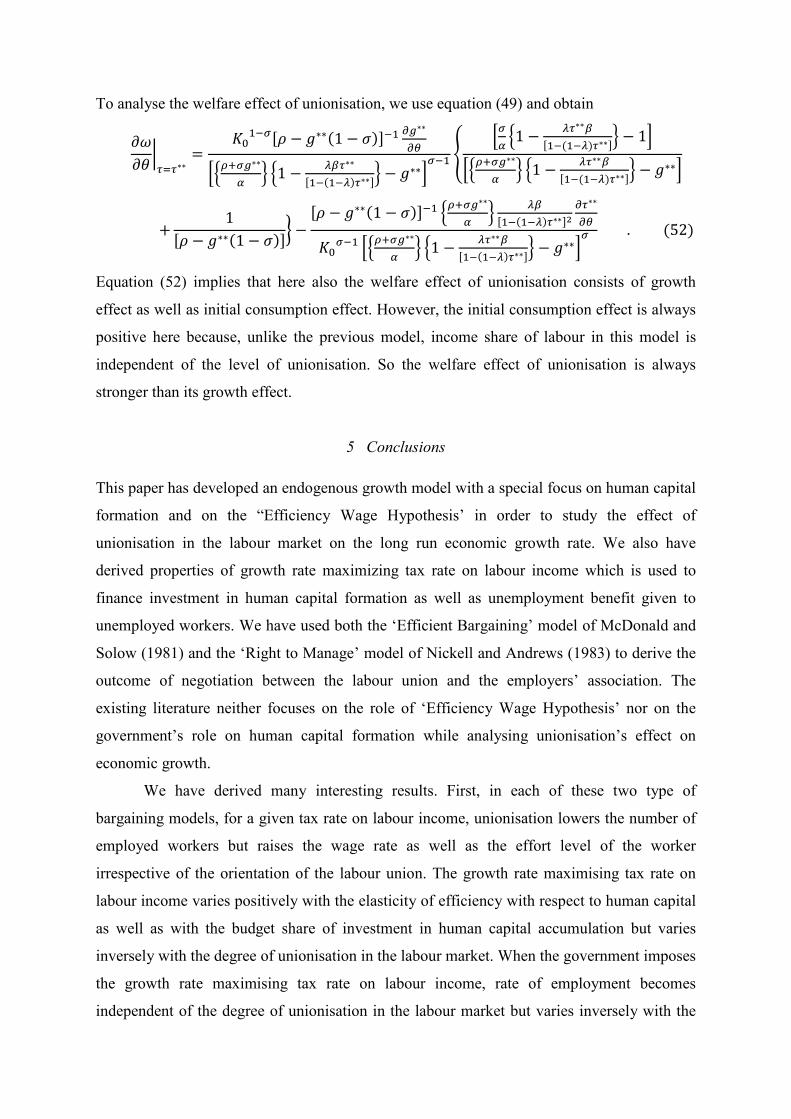
purpose, we differentiate 𝜔𝜔 with respect to τ at 𝜏𝜏 = 𝜏𝜏∗ and obtain

𝜕𝜕𝜔𝜔𝜕𝜕𝜏𝜏�𝜏𝜏=𝜏𝜏∗

= −𝐾𝐾01−𝜎𝜎 �

𝜌𝜌+𝜎𝜎𝜎𝜎∗

𝛼𝛼� � [𝜃𝜃𝑛𝑛(1−𝛼𝛼)+𝛽𝛽(1−𝜃𝜃)]𝜆𝜆

(1−𝜃𝜃+𝜃𝜃𝑛𝑛)[1−(1−𝜆𝜆)τ∗]2� [𝜌𝜌 − 𝑔𝑔∗(1 − 𝜎𝜎)]−1

��𝜌𝜌+𝜎𝜎𝜎𝜎∗

𝛼𝛼� �1 − 𝜆𝜆𝜏𝜏∗

[1−(1−𝜆𝜆)𝜏𝜏∗][𝜃𝜃𝑛𝑛(1−𝛼𝛼)+𝛽𝛽(1−𝜃𝜃)]

(1−𝜃𝜃+𝜃𝜃𝑛𝑛) � − 𝑔𝑔∗�𝜎𝜎 < 0 . (36)

Here 𝑔𝑔∗ = 𝑔𝑔|𝜏𝜏=𝜏𝜏∗. Equation (36) implies that the welfare maximising tax rate on labour

income is lower than the growth rate maximising tax rate. This is so because, given the

allocation of tax revenue between investment in human capital accumulation and

unemployment subsidy, initial consumption level of the representative household falls with

increase in the labour income tax rate. Since the economic growth rate in the steady state

equilibrium does not depend on the level of initial consumption34, so the growth rate

maximising tax rate, 𝜏𝜏∗, does not take into account this negative effect of taxation on initial

consumption. On the other hand, welfare level depends on the level of initial consumption;

and so the welfare maximising labour income tax rate takes into account this negative effect.

This result is stated in the following proposition.

Proposition 4: Welfare maximising tax rate on labour income is lower than the

corresponding growth rate maximising tax rate in the presence of public investment in human

capital accumulation.

3.3 Effect of unionisation

34 See equation (31).

We now turn to analyse the effect of an increase in 𝜃𝜃 on the endogenous growth rate when

the government charges the growth rate maximising labour income tax rate35. Using

equations (31) and (32), we obtain

(𝜌𝜌 + 𝜎𝜎𝑔𝑔∗)[𝑔𝑔∗]𝛽𝛽𝛽𝛽

1−𝛽𝛽𝛽𝛽

= 𝐴𝐴1

1−𝛽𝛽𝛽𝛽𝛼𝛼(1 − 𝜂𝜂)𝛽𝛽

1−𝛽𝛽𝛽𝛽[𝛩𝛩1]𝛽𝛽𝛽𝛽

1−𝛽𝛽𝛽𝛽 �𝜂𝜂𝜆𝜆[𝜃𝜃𝑛𝑛(1 − 𝛼𝛼) + 𝛽𝛽(1 − 𝜃𝜃)]

(1 − 𝜂𝜂)𝛩𝛩1(1 − 𝜆𝜆)(1 − 𝜃𝜃 + 𝜃𝜃𝑛𝑛)�

𝛽𝛽𝛽𝛽1−𝛽𝛽𝛽𝛽

. (37)

From equation (37), we have

�𝜎𝜎𝑔𝑔∗

(𝜌𝜌 + 𝜎𝜎𝑔𝑔∗) +𝛽𝛽𝜂𝜂

1 − 𝛽𝛽𝜂𝜂�𝜕𝜕𝜎𝜎∗

𝜕𝜕𝜃𝜃𝑔𝑔∗

= �𝛽𝛽𝜂𝜂

1 − 𝛽𝛽𝜂𝜂� �

𝑛𝑛(1 − 𝛼𝛼 − 𝛽𝛽)(1 − 𝜃𝜃 + 𝜃𝜃𝑛𝑛)[𝜃𝜃𝑛𝑛(1 − 𝛼𝛼) + 𝛽𝛽(1 − 𝜃𝜃)]�

−𝛽𝛽2𝑚𝑚𝜂𝜂(1 − 𝛼𝛼 − 𝛽𝛽)(1 − 𝛿𝛿)

(1 − 𝛽𝛽𝜂𝜂)[𝜃𝜃(𝑛𝑛 −𝑚𝑚)(1 − 𝛼𝛼 − 𝛽𝛽) + 𝛽𝛽(1 − 𝛿𝛿)(1 − 𝜃𝜃 + 𝜃𝜃𝑛𝑛)]2

+𝛽𝛽2𝑚𝑚𝛿𝛿(1 − 𝛼𝛼 − 𝛽𝛽)(1 − 𝛿𝛿)

(1 − 𝛽𝛽𝜂𝜂)[𝜃𝜃(𝑛𝑛 −𝑚𝑚)(1 − 𝛼𝛼 − 𝛽𝛽) + 𝛽𝛽(1 − 𝛿𝛿)(1 − 𝜃𝜃 + 𝜃𝜃𝑛𝑛)]2 . (38)

Equation (38) shows that the growth effect of unionisation is ambiguous. It consists of two

effects – (i) the effort effect and (ii) the human capital accumulation effect. The first effect is

operated through the change in the effort level of the worker. It is positive and is captured by

the third term in the R.H.S. of equation (38). The second effect is operated through the

change in the rate of human capital accumulation. It is ambiguous in sign and is captured by

the first term as well as by the second term in the R.H.S. of equation (38). On the one hand,

unionisation raises labour share of income and thereby the tax base36. This positive effect is

captured by the first term. However, on the other hand, unionisation lowers the growth rate

maximising tax rate; and this negative effect is captured by the second term. So the net effect

on tax revenue generation is ambiguous. Since a fixed fraction of tax revenue is spent to

finance human capital accumulation, the effect on human capital accumulation is also

ambiguous. If human capital is not productive, i.e., if 𝜂𝜂 = 0, then only the positive effort

effect remains and unionisation always raises the rate of economic growth. Similarly, if the

effort level is independent of the wage rate, i.e., if 𝛿𝛿 = 0, then the third term is vanished and

the effect of unionisation depends only on the human capital accumulation effect. However,

if we ignore the entire dynamic ‘Efficiency Wage Hypothesis’, i.e., if we assume that 𝛿𝛿 =

35 Since we cannot derive the welfare maximising labour income tax rate, so we are unable to derive the growth effect of unionisation when the government charges the welfare maximising labour income tax rate. 36 See footnote 23.

𝜂𝜂 = 0, then unionisation does not affect the growth rate of the economy. This result is valid

regardless of the nature of orientation of the labour union. This happens because unionisation

does not affect the level of employment when government chooses the growth rate

maximising tax rate.

Combining the second and the third term in the R.H.S. of equation (38), we find that

the positive work effort effect dominates the negative component of human capital

accumulation effect if the elasticity of worker’s efficiency with respect to the wage premium

rate, 𝛿𝛿, is higher than the elasticity of worker’s efficiency with respect to the stock of human

capital, 𝜂𝜂. So unionisation in this case is definitely growth generating as the other component

of human capital accumulation effect is always positive. However, the converse is not

necessarily true. So, 𝛿𝛿 > 𝜂𝜂 is a sufficient condition but not a necessary condition to ensure

positive growth effect of unionisation. These results are summarised in the following

proposition.

Proposition 5: Growth effect of unionisation consists of a positive work effort effect and an

ambiguous human capital accumulation effect. If the elasticity of worker’s efficiency with

respect to the stock of human capital is not higher than the elasticity of worker’s efficiency

with respect to the wage premium, then unionisation always raises the economic growth rate.

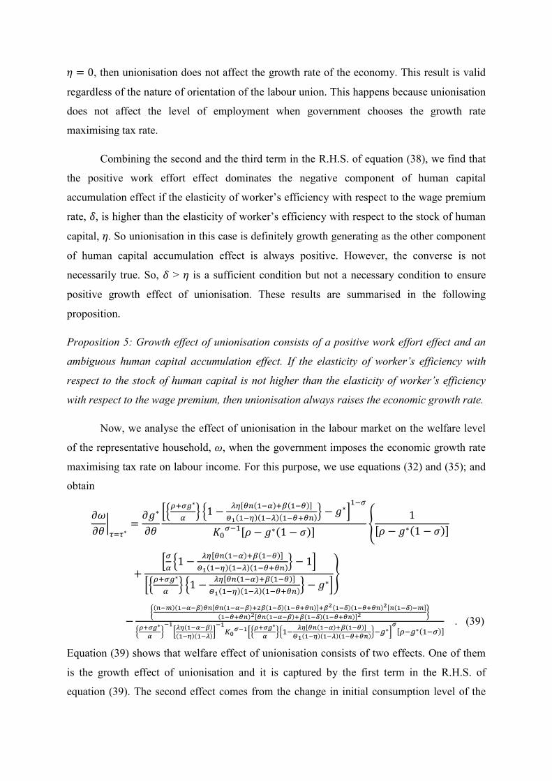
Now, we analyse the effect of unionisation in the labour market on the welfare level

of the representative household, ω, when the government imposes the economic growth rate

maximising tax rate on labour income. For this purpose, we use equations (32) and (35); and

obtain

𝜕𝜕𝜔𝜔𝜕𝜕𝜃𝜃�𝜏𝜏=𝜏𝜏∗

=𝜕𝜕𝑔𝑔∗

𝜕𝜕𝜃𝜃

��𝜌𝜌+𝜎𝜎𝜎𝜎∗

𝛼𝛼� �1 − 𝜆𝜆𝜂𝜂[𝜃𝜃𝑛𝑛(1−𝛼𝛼)+𝛽𝛽(1−𝜃𝜃)]

𝛩𝛩1(1−𝜂𝜂)(1−𝜆𝜆)(1−𝜃𝜃+𝜃𝜃𝑛𝑛)� − 𝑔𝑔∗�1−𝜎𝜎

𝐾𝐾0𝜎𝜎−1[𝜌𝜌 − 𝑔𝑔∗(1 − 𝜎𝜎)]�

1[𝜌𝜌 − 𝑔𝑔∗(1 − 𝜎𝜎)]

+�𝜎𝜎𝛼𝛼�1 − 𝜆𝜆𝜂𝜂[𝜃𝜃𝑛𝑛(1−𝛼𝛼)+𝛽𝛽(1−𝜃𝜃)]

𝛩𝛩1(1−𝜂𝜂)(1−𝜆𝜆)(1−𝜃𝜃+𝜃𝜃𝑛𝑛)� − 1�

��𝜌𝜌+𝜎𝜎𝜎𝜎∗

𝛼𝛼� �1 − 𝜆𝜆𝜂𝜂[𝜃𝜃𝑛𝑛(1−𝛼𝛼)+𝛽𝛽(1−𝜃𝜃)]

𝛩𝛩1(1−𝜂𝜂)(1−𝜆𝜆)(1−𝜃𝜃+𝜃𝜃𝑛𝑛)� − 𝑔𝑔∗��

−�(𝑛𝑛−𝑚𝑚)(1−𝛼𝛼−𝛽𝛽)𝜃𝜃𝑛𝑛[𝜃𝜃𝑛𝑛(1−𝛼𝛼−𝛽𝛽)+2𝛽𝛽(1−𝛽𝛽)(1−𝜃𝜃+𝜃𝜃𝑛𝑛)]+𝛽𝛽2(1−𝛽𝛽)(1−𝜃𝜃+𝜃𝜃𝑛𝑛)2[𝑛𝑛(1−𝛽𝛽)−𝑚𝑚]

(1−𝜃𝜃+𝜃𝜃𝑛𝑛)2[𝜃𝜃𝑛𝑛(1−𝛼𝛼−𝛽𝛽)+𝛽𝛽(1−𝛽𝛽)(1−𝜃𝜃+𝜃𝜃𝑛𝑛)]2 �

�𝜌𝜌+𝜎𝜎𝑔𝑔∗

𝛼𝛼 �−1�𝜆𝜆𝛽𝛽(1−𝛼𝛼−𝛽𝛽)

(1−𝛽𝛽)(1−𝜆𝜆)�−1𝐾𝐾0𝜎𝜎−1��

𝜌𝜌+𝜎𝜎𝑔𝑔∗𝛼𝛼 ��1− 𝜆𝜆𝛽𝛽[𝜃𝜃𝑛𝑛(1−𝛼𝛼)+𝛽𝛽(1−𝜃𝜃)]

𝛩𝛩1(1−𝛽𝛽)(1−𝜆𝜆)(1−𝜃𝜃+𝜃𝜃𝑛𝑛)�−𝜎𝜎∗�𝜎𝜎

[𝜌𝜌−𝜎𝜎∗(1−𝜎𝜎)] . (39)

Equation (39) shows that welfare effect of unionisation consists of two effects. One of them

is the growth effect of unionisation and it is captured by the first term in the R.H.S. of

equation (39). The second effect comes from the change in initial consumption level of the

household due to change in the educational expenditure; and it is captured by the second term

in the R.H.S. of equation (39). This effect is ambiguous because the term �(𝑛𝑛 −𝑚𝑚)(1 − 𝛼𝛼 −

𝛽𝛽)𝜃𝜃𝑛𝑛[𝜃𝜃𝑛𝑛(1 − 𝛼𝛼 − 𝛽𝛽) + 2𝛽𝛽(1 − 𝛿𝛿)(1 − 𝜃𝜃 + 𝜃𝜃𝑛𝑛)] + 𝛽𝛽2(1 − 𝛿𝛿)(1 − 𝜃𝜃 + 𝜃𝜃𝑛𝑛)2[𝑛𝑛(1 − 𝛿𝛿) −

𝑚𝑚]� is ambiguous in sign. This is so because, on the one hand, unionisation lowers the tax

rate and thereby lowers investment in human capital accumulation. This can be easily

understood from the term 𝜆𝜆τ [1 − (1 − 𝜆𝜆)τ]⁄ in the R.H.S. of equation (35). On the other

hand, unionisation raises the income share of labour and thereby the tax base. This can be

easily understood from the term [𝜃𝜃𝑛𝑛(1 − 𝛼𝛼) + 𝛽𝛽(1 − 𝜃𝜃)] (1 − 𝜃𝜃 + 𝜃𝜃𝑛𝑛)⁄ in the R.H.S. of

equation (35). So if m ≥ n, then the effect on tax rate dominates the other effect and the initial

consumption effect becomes positive. So the welfare effect of unionisation is stronger than its

growth effect in this case. The major result is stated in the following proposition.

Proposition 6: The welfare effect of unionisation is different from its growth effect when the

government invests in human capital accumulation; and is stronger than the growth effect if

m ≥ n.

In Chang et al. (2007), growth effect as well as welfare effect of unionisation solely

consists of the employment effect of unionisation, which depends only on the orientation of

the labour union. However, there is no employment effect in our model; and hence the

growth effect as well as the welfare effect of unionisation does not depend on the orientation

of labour union.

We now contrast our result to the related results of existing literature. In Palokangas

(1996), unionisation reduces employment of both unskilled labour and skilled labour in

production of the final good due to their complementary relationship; and this leads to a rise

in the employment of skilled labour in the R&D sector and therefore raises the growth rate. In

Sorensen (1997), on the one hand, unionization raises the skill of the workers, but, on the

other hand, lowers the profit and, in turn, the marginal return from skill accumulation. The

growth rate is reduced (increased) in the ‘Efficient Bargaining’ model (‘Right to manage

model’). Bräuninger (2000b) shows that, in general, unionisation dampens capital

accumulation and thereby growth. Lingens (2003a) shows in a creative destruction growth

model that, unionisation lessens the expected profit of the innovators and employment of

skilled labour in the manufacturing sector. This surplus labour is absorbed in the R&D sector

and rate of innovation is raised. So the aggregate effect on growth is indeterminate and

depends on the elasticity of substitution between the two types of labour in the manufacturing

sector. In an OLG model, Irmen and Wigger (2002/2003) shows that unionisation causes a

transfer of income from the dissaving old to the saving young. This raises capital

accumulation and thereby raises growth. In Lingens (2003b), skill formation is endogenous;

and due to unionisation in the unskilled labour market, the skilled unskilled relative wage

ratio falls and thus the supply of skilled labour goes down. If the long-run equilibrium level

of skilled workers is low (high), then unionisation lowers (raises) the economic growth rate.

Lai and Wang (2010) shows that unionisation raises (lowers) the growth rate if and only if the

balanced growth equilibrium is locally determinate (indeterminate). In Adjemian et al.

(2010), unionization reduces profit and thus reduces the expected value of innovation; and

thereby discourages R&D and economic growth. However, our result is different from the

above results and none of these above mentioned works considers the role of dynamic

efficiency of workers.

4 Negotiation with ‘Right to Manage’ model

In this case, the employers’ union and the employees’ union bargain only over the

wage rate; and the firm determines the number of employed workers from its labour demand

function obtained from its profit maximisation exercise. So, from equations (1), (2), (2.a),

(2.b) and (3), we obtain the inverted labour demand function of the representative firm as

given by

𝑤𝑤 = �𝛽𝛽𝐴𝐴𝐾𝐾𝛼𝛼𝐾𝐾�𝛾𝛾𝑒𝑒𝛽𝛽−1ℎ𝛽𝛽𝜂𝜂𝑏𝑏−𝛽𝛽𝛿𝛿�1

1−𝛽𝛽𝛽𝛽 . (40)

So the firms’ association and the labour union jointly maximise the ‘generalised Nash

product’ function given by equation (9) with respect to w only subject to equation (40). Using

the first order condition of maximisation and equations (1), (2), (2.a), (2.b), (4), (6) and (40),

optimum values of L and 𝑤𝑤 are obtained as37

𝑒𝑒∗∗ = [1−𝜏𝜏(1−𝜆𝜆)]{𝜃𝜃𝑛𝑛(1−𝛼𝛼−𝛽𝛽)(1−𝛽𝛽𝛿𝛿)+𝛽𝛽(1−𝛿𝛿)(1−𝜃𝜃)(1−𝛽𝛽)−𝜃𝜃𝑚𝑚(1−𝛽𝛽)(1−𝛼𝛼−𝛽𝛽)}{𝜃𝜃𝑛𝑛(1−𝛼𝛼−𝛽𝛽)(1−𝛽𝛽𝛿𝛿)+𝛽𝛽(1−𝛿𝛿)(1−𝜃𝜃)(1−𝛽𝛽)}−[1−𝜏𝜏(1−𝜆𝜆)]𝜃𝜃𝑚𝑚(1−𝛽𝛽)(1−𝛼𝛼−𝛽𝛽) < 1 ; (41)

and

𝑤𝑤∗∗ = 𝛽𝛽𝐴𝐴𝐾𝐾𝛼𝛼𝐾𝐾�𝛾𝛾ℎ𝛽𝛽𝜂𝜂𝑒𝑒∗∗𝛽𝛽−1−𝛽𝛽𝛿𝛿𝜏𝜏−𝛽𝛽𝛿𝛿(1 − 𝑒𝑒∗∗)𝛽𝛽𝛿𝛿(1 − 𝜆𝜆)−𝛽𝛽𝛿𝛿[1 − 𝜏𝜏(1 − 𝜆𝜆)]𝛽𝛽𝛿𝛿 . (42)

We assume the following parametric restriction to be valid in order to ensure that 𝑒𝑒∗∗ > 0.

{𝜃𝜃𝑛𝑛(1 − 𝛼𝛼 − 𝛽𝛽)(1 − 𝛽𝛽𝛿𝛿) + 𝛽𝛽(1 − 𝛿𝛿)(1− 𝜃𝜃)(1 − 𝛽𝛽)} > 𝜃𝜃𝑚𝑚(1 − 𝛽𝛽)(1− 𝛼𝛼 − 𝛽𝛽) .

37 Derivations of equations (41), (42) and (44) are provided in appendix E. We assume that second order condition of maximisation is satisfied.

This restriction implies that the labour union can not be highly wage oriented. In this model

also, 𝑒𝑒∗ varies inversely with 𝜃𝜃 when τ and λ are given. This is shown by

𝜕𝜕𝐿𝐿∗∗

𝜕𝜕𝜃𝜃= − [1−(1−𝜆𝜆)𝜏𝜏](1−𝜆𝜆)𝜏𝜏𝛽𝛽𝑚𝑚(1−𝛽𝛽)2(1−𝛼𝛼−𝛽𝛽)(1−𝛿𝛿)

[{𝜃𝜃𝑛𝑛(1−𝛼𝛼−𝛽𝛽)(1−𝛽𝛽𝛿𝛿)+𝛽𝛽(1−𝛿𝛿)(1−𝜃𝜃)(1−𝛽𝛽)}−[1−𝜏𝜏(1−𝜆𝜆)]𝜃𝜃𝑚𝑚(1−𝛽𝛽)(1−𝛼𝛼−𝛽𝛽)]2 < 0 . (43)

Now, from equations (2.b), (6) and (41), representative worker’s effort level is

obtained and is given by

𝑒𝑒2∗∗ = �[1 − (1 − 𝜆𝜆)𝜏𝜏](1 − 𝑒𝑒∗∗)

(1 − 𝜆𝜆)𝜏𝜏𝑒𝑒∗∗�𝛿𝛿

= � {𝜃𝜃𝑛𝑛(1−𝛼𝛼−𝛽𝛽)(1−𝛽𝛽𝛿𝛿)+𝛽𝛽(1−𝛿𝛿)(1−𝜃𝜃)(1−𝛽𝛽)}{𝜃𝜃𝑛𝑛(1−𝛼𝛼−𝛽𝛽)(1−𝛽𝛽𝛿𝛿)+𝛽𝛽(1−𝛿𝛿)(1−𝜃𝜃)(1−𝛽𝛽)−𝜃𝜃𝑚𝑚(1−𝛽𝛽)(1−𝛼𝛼−𝛽𝛽)}�

𝛿𝛿 . (44)

From equation (44), we have

𝜕𝜕𝑒𝑒2∗∗

𝜕𝜕𝜃𝜃= 𝛿𝛿{𝜃𝜃𝑛𝑛(1−𝛼𝛼−𝛽𝛽)(1−𝛽𝛽𝛿𝛿)+𝛽𝛽(1−𝛿𝛿)(1−𝜃𝜃)(1−𝛽𝛽)}𝛽𝛽−1𝛽𝛽𝑚𝑚(1−𝛽𝛽)2(1−𝛼𝛼−𝛽𝛽)(1−𝛿𝛿)

[𝜃𝜃𝑛𝑛(1−𝛼𝛼−𝛽𝛽)(1−𝛽𝛽𝛿𝛿)+𝛽𝛽(1−𝛿𝛿)(1−𝜃𝜃)(1−𝛽𝛽)−𝜃𝜃𝑚𝑚(1−𝛽𝛽)(1−𝛼𝛼−𝛽𝛽)]𝛽𝛽+1 > 0 . (45)

Equation (45) implies that effort level of the worker varies positively with the degree of

unionisation. Since, in this model, the government’s budget balancing equations as well as

the representative household’s behaviour are identical to those given in the ‘Efficient

Bargaining’ model, so the existence and stability properties of the steady state equilibrium

derived in that model will remain unchanged here.

Now, using equations (2), (2.a), (2.b), (5), (6), (23), (42) and (44), we obtain the

balanced growth equation given by

(𝜌𝜌 + 𝜎𝜎𝑔𝑔)[𝑔𝑔]𝛽𝛽𝛽𝛽

1−𝛽𝛽𝛽𝛽 = 𝐴𝐴1

1−𝛽𝛽𝛽𝛽𝛼𝛼𝑒𝑒∗∗𝛽𝛽(1−𝛽𝛽)1−𝛽𝛽𝛽𝛽 �(1−𝐿𝐿∗∗)

(1−𝜆𝜆) �𝛽𝛽𝛽𝛽

1−𝛽𝛽𝛽𝛽 [𝛽𝛽𝜆𝜆]𝛽𝛽𝛽𝛽

1−𝛽𝛽𝛽𝛽 �[1−(1−𝜆𝜆)𝜏𝜏]𝜏𝜏

�𝛽𝛽𝛽𝛽−𝛽𝛽𝛽𝛽1−𝛽𝛽𝛽𝛽 . (46)

Using equations (41) and (46), we obtain the growth rate maximising tax rate given by

𝜏𝜏∗∗ = 𝜂𝜂{𝜃𝜃𝑛𝑛(1−𝛼𝛼−𝛽𝛽)(1−𝛽𝛽𝛿𝛿)+𝛽𝛽(1−𝛿𝛿)(1−𝜃𝜃)(1−𝛽𝛽)−𝜃𝜃𝑚𝑚(1−𝛽𝛽)(1−𝛼𝛼−𝛽𝛽)}{𝜃𝜃𝑛𝑛(1−𝛼𝛼−𝛽𝛽)(1−𝛽𝛽𝛿𝛿)+𝛽𝛽(1−𝛿𝛿)(1−𝜃𝜃)(1−𝛽𝛽)−𝜂𝜂𝜃𝜃𝑚𝑚(1−𝛽𝛽)(1−𝛼𝛼−𝛽𝛽)}(1−𝜆𝜆)

. (47)

From equation (47), we obtain

𝜕𝜕𝜏𝜏∗∗

𝜕𝜕𝜃𝜃= − 𝜂𝜂(1−𝜂𝜂)𝛽𝛽𝑚𝑚(1−𝛽𝛽)2(1−𝛼𝛼−𝛽𝛽)(1−𝛿𝛿)

{𝜃𝜃𝑛𝑛(1−𝛼𝛼−𝛽𝛽)(1−𝛽𝛽𝛿𝛿)+𝛽𝛽(1−𝛿𝛿)(1−𝜃𝜃)(1−𝛽𝛽)−𝜂𝜂𝜃𝜃𝑚𝑚(1−𝛽𝛽)(1−𝛼𝛼−𝛽𝛽)}2(1−𝜆𝜆) < 0 . (48)

So the growth rate maximising tax rate varies inversely with the degree of unionisation.

Incorporating the value of 𝜏𝜏∗∗ from equation (47) in equation (41), we obtain the same value

of 𝑒𝑒∗∗ as that is given in equation (34). Now, to check the equivalence between the growth

rate maximising labour income tax rate and the welfare maximising labour income tax rate,

we use equations (1), (3), (6), (21), (22), (23) and (40); and thus obtain

𝜔𝜔 =𝐾𝐾01−𝜎𝜎 ��

𝜌𝜌+𝜎𝜎𝜎𝜎𝛼𝛼� �1 − 𝜆𝜆τ𝛽𝛽

[1−(1−𝜆𝜆)τ]� − 𝑔𝑔�1−𝜎𝜎

(1 − 𝜎𝜎)[𝜌𝜌 − 𝑔𝑔(1 − 𝜎𝜎)] + 𝑐𝑐𝑐𝑐𝑛𝑛𝑐𝑐𝑑𝑑𝑎𝑎𝑛𝑛𝑑𝑑 . (49)

We assume 1 > σ and ρ > g(1-σ). Since initial consumption, 𝑐𝑐0, is positive, so �𝜌𝜌+𝜎𝜎𝜎𝜎𝛼𝛼� �1 −

𝜆𝜆τ𝛽𝛽[1−(1−𝜆𝜆)τ]� has to be greater than g. From equation (49), we obtain

𝜕𝜕𝜔𝜔𝜕𝜕𝜏𝜏�𝜏𝜏=𝜏𝜏∗∗

= −𝐾𝐾01−𝜎𝜎 �

𝜌𝜌+𝜎𝜎𝜎𝜎∗∗

𝛼𝛼� � 𝛽𝛽𝜆𝜆

[1−(1−𝜆𝜆)𝜏𝜏∗∗]2�

��𝜌𝜌+𝜎𝜎𝜎𝜎∗∗

𝛼𝛼� �1 − 𝜆𝜆𝜏𝜏∗∗𝛽𝛽

[1−(1−𝜆𝜆)𝜏𝜏∗∗]� − 𝑔𝑔∗∗�𝜎𝜎

[𝜌𝜌 − 𝑔𝑔∗∗(1 − 𝜎𝜎)]< 0 ; (50)

Equation (50) shows that here also the welfare maximising tax rate falls short of the growth

rate maximising tax rate due to the negative effect of taxation on initial consumption.

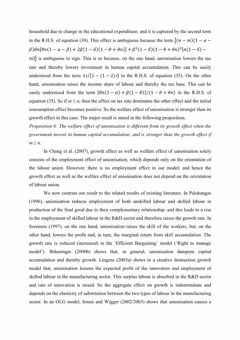
Now, using equations (34), (46) and (47), we obtain

� 𝜎𝜎𝜎𝜎∗∗

(𝜌𝜌+𝜎𝜎𝜎𝜎∗∗) + 𝛽𝛽𝜂𝜂1−𝛽𝛽𝜂𝜂

�𝜕𝜕𝑔𝑔∗∗

𝜕𝜕𝜃𝜃𝜎𝜎∗∗

= −�𝛽𝛽[𝛿𝛿−𝜂𝜂]1−𝛽𝛽𝜂𝜂

� � (1−𝜆𝜆)[1−(1−𝜆𝜆)𝜏𝜏∗∗] + 1

𝜏𝜏∗∗� 𝜕𝜕𝜏𝜏

∗∗

𝜕𝜕𝜃𝜃⋛ 0 𝑖𝑖𝑖𝑖𝑖𝑖 𝛿𝛿 ⋛ 𝜂𝜂 . (51)

Equation (51) shows that the sign of the growth effect of unionisation depends solely on the

sign of (𝛿𝛿 − 𝜂𝜂). So, if the elasticity of worker’s efficiency with respect to the wage premium,

δ, is higher than (equal to) (lower than) the elasticity of worker’s efficiency with respect to

the stock of human capital, η, then unionisation in the labour market raises (does not affect)

(lowers) the rate of economic growth. In the ‘Efficient Bargaining’ model, the growth effect

of unionisation partially depends on the mathematical sign of (𝛿𝛿 − 𝜂𝜂). However, in the

‘Right to Manage’ model, growth effect of unionisation fully depends on the mathematical

sign of (𝛿𝛿 − 𝜂𝜂). So in this model, δ > η is a necessary as well as a sufficient condition to

ensure positive growth effect of unionisation. Important results derived in this section are

summarized in the following proposition.

Proposition 7: In the ‘Right to Manage’ model of bargaining, unionisation in the labour

market raises (does not change) (lowers) the rate of economic growth if the elasticity of

worker’s efficiency with respect to the wage premium is higher than (equal to) (lower than)

the elasticity of worker’s efficiency with respect to the stock of human capital.

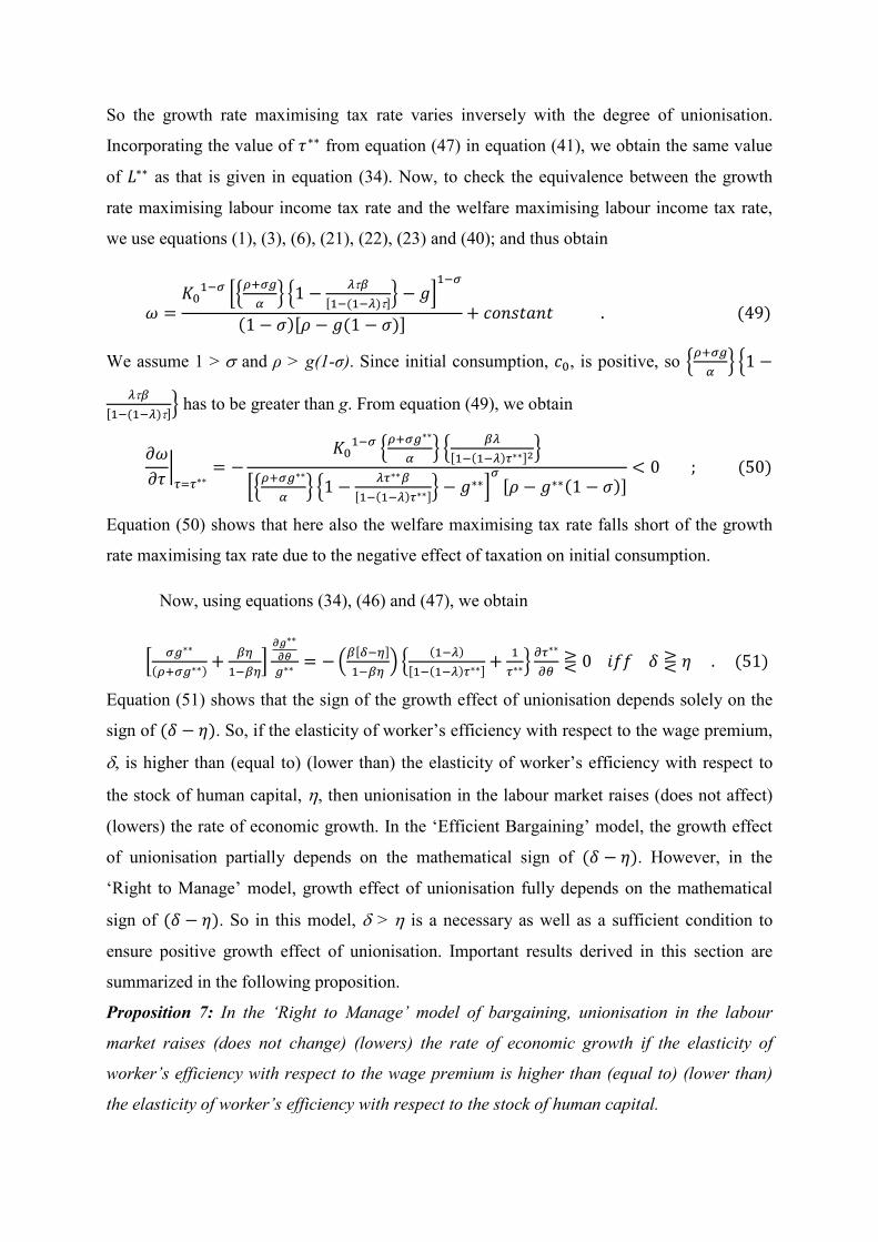
To analyse the welfare effect of unionisation, we use equation (49) and obtain

𝜕𝜕𝜔𝜔𝜕𝜕𝜃𝜃�𝜏𝜏=𝜏𝜏∗∗

=𝐾𝐾01−𝜎𝜎[𝜌𝜌 − 𝑔𝑔∗∗(1 − 𝜎𝜎)]−1 𝜕𝜕𝜎𝜎

∗∗

𝜕𝜕𝜃𝜃

��𝜌𝜌+𝜎𝜎𝜎𝜎∗∗

𝛼𝛼� �1 − 𝜆𝜆𝛽𝛽𝜏𝜏∗∗

[1−(1−𝜆𝜆)𝜏𝜏∗∗]� − 𝑔𝑔∗∗�𝜎𝜎−1 �

�𝜎𝜎𝛼𝛼�1 − 𝜆𝜆𝜏𝜏∗∗𝛽𝛽

[1−(1−𝜆𝜆)𝜏𝜏∗∗]� − 1�

��𝜌𝜌+𝜎𝜎𝜎𝜎∗∗

𝛼𝛼� �1 − 𝜆𝜆𝜏𝜏∗∗𝛽𝛽

[1−(1−𝜆𝜆)𝜏𝜏∗∗]� − 𝑔𝑔∗∗�

+1

[𝜌𝜌 − 𝑔𝑔∗∗(1 − 𝜎𝜎)]� −[𝜌𝜌 − 𝑔𝑔∗∗(1 − 𝜎𝜎)]−1 �𝜌𝜌+𝜎𝜎𝜎𝜎

∗∗

𝛼𝛼� 𝜆𝜆𝛽𝛽

[1−(1−𝜆𝜆)𝜏𝜏∗∗]2𝜕𝜕𝜏𝜏∗∗

𝜕𝜕𝜃𝜃

𝐾𝐾0𝜎𝜎−1 ��𝜌𝜌+𝜎𝜎𝜎𝜎∗∗

𝛼𝛼� �1 − 𝜆𝜆𝜏𝜏∗∗𝛽𝛽

[1−(1−𝜆𝜆)𝜏𝜏∗∗]� − 𝑔𝑔∗∗�𝜎𝜎 . (52)

Equation (52) implies that here also the welfare effect of unionisation consists of growth

effect as well as initial consumption effect. However, the initial consumption effect is always

positive here because, unlike the previous model, income share of labour in this model is

independent of the level of unionisation. So the welfare effect of unionisation is always

stronger than its growth effect.

5 Conclusions

This paper has developed an endogenous growth model with a special focus on human capital

formation and on the “Efficiency Wage Hypothesis’ in order to study the effect of

unionisation in the labour market on the long run economic growth rate. We also have

derived properties of growth rate maximizing tax rate on labour income which is used to

finance investment in human capital formation as well as unemployment benefit given to

unemployed workers. We have used both the ‘Efficient Bargaining’ model of McDonald and

Solow (1981) and the ‘Right to Manage’ model of Nickell and Andrews (1983) to derive the

outcome of negotiation between the labour union and the employers’ association. The

existing literature neither focuses on the role of ‘Efficiency Wage Hypothesis’ nor on the

government’s role on human capital formation while analysing unionisation’s effect on

economic growth.

We have derived many interesting results. First, in each of these two type of

bargaining models, for a given tax rate on labour income, unionisation lowers the number of

employed workers but raises the wage rate as well as the effort level of the worker

irrespective of the orientation of the labour union. The growth rate maximising tax rate on

labour income varies positively with the elasticity of efficiency with respect to human capital

as well as with the budget share of investment in human capital accumulation but varies

inversely with the degree of unionisation in the labour market. When the government imposes

the growth rate maximising tax rate on labour income, rate of employment becomes

independent of the degree of unionisation in the labour market but varies inversely with the

elasticity of efficiency with respect to human capital. Secondly, the growth rate maximising

tax rate on labour income is different from the corresponding welfare maximising tax rate.

The Welfare effect of unionisation is also different from the growth effect of unionisation in

both these two models. Thirdly, in case of the ‘Efficient Bargaining’ model, if the elasticity

of worker’s effort level with respect to the wage premium is higher than the elasticity of

worker’s efficiency with respect to the stock of human capital, then there exists a positive

growth effect of unionisation in the labour market though this condition is not necessary.

However, in case of the ‘Right to Manage’ model, this condition becomes necessary as well

as sufficient to obtain a positive growth effect of unionisation. These results stand on a sharp

contrast to those of the existing literature.

However, our simple theoretical model does not consider many important aspects of

reality. Issues like population growth, technological progress, positive externality of public

goods etc. are ignored for the sake of simplicity. We also do not consider capital income

taxation for analytical simplicity. We only focuses on publicly financed education and not on

privately financed education. So, household’s income allocation towards education, is not

considered here. To avoid complexity in the theoretical analysis, we assume ‘closed shop

labour union’, rather than the more common ‘open shop labour union’. The labour union’s

simple utility function does not take care of its other priorities like workplace safety and

environmental issues. We plan to do further research in future removing these limitations.

Appendix

Appendix A: Derivation of optimal w and L

From equations (4) and (10), we obtain

𝜃𝜃𝑚𝑚[(1 − 𝛼𝛼)𝑌𝑌 − 𝑤𝑤𝑒𝑒] = (1 − 𝜃𝜃)(𝑤𝑤 − 𝑏𝑏) �𝑒𝑒 −𝛽𝛽𝛿𝛿𝑌𝑌𝑤𝑤

� . (𝐴𝐴. 1)

Now from equation (6), we obtain

𝑏𝑏(1 − 𝑒𝑒) =(1 − 𝜆𝜆)τ𝑤𝑤𝑒𝑒

[1 − (1 − 𝜆𝜆)τ] . (𝐴𝐴. 2)

Using equations (A.1) and (A.2), we obtain

𝜃𝜃𝑚𝑚[(1 − 𝛼𝛼)𝑌𝑌 − 𝑤𝑤𝑒𝑒] = (1 − 𝜃𝜃) �𝑤𝑤 −(1 − 𝜆𝜆)τ𝑤𝑤𝑒𝑒

[1 − (1 − 𝜆𝜆)τ](1 − 𝑒𝑒)� �𝑒𝑒 −𝛽𝛽𝛿𝛿𝑌𝑌𝑤𝑤

� . (𝐴𝐴. 3)

Using equations (11.a) and (A.3), we obtain

(1 − 𝑒𝑒)[1 − (1 − 𝜆𝜆)τ]

(1 − 𝜆𝜆)τ𝑒𝑒= 𝛩𝛩1 . (𝐴𝐴. 4)

From equation (A.4), we obtain equation (12) in the body of the article.

Incorporating the value of 𝑒𝑒∗ from equation (12) in equation (A.2), we obtain equation (13) in

the body of the article. We assume that second order conditions of maximisation is satisfied.

Appendix B: Derivation of equation (23)

Using equations (21) and (22), we construct the Current Value Hamiltonian as given by

𝐻𝐻𝑐𝑐 =𝑐𝑐1−𝜎𝜎 − 1

1 − 𝜎𝜎+ 𝜇𝜇[(1 − 𝜏𝜏)𝑤𝑤𝑒𝑒 + 𝑟𝑟𝐾𝐾 + 𝜋𝜋 + (1 − 𝜏𝜏)𝑏𝑏(1 − 𝑒𝑒) − 𝑐𝑐] . (𝐵𝐵. 1)

Here 𝜇𝜇 is the co-state variable. Maximising equation (B.1) with respect to c, we obtain the

following first order condition.

𝑐𝑐−𝜎𝜎 − 𝜇𝜇 = 0 ; (𝐵𝐵. 2)

Again from equation (B.1), we have

��𝜇𝜇𝜇

= 𝜌𝜌 − 𝑟𝑟 ; (𝐵𝐵. 3)

and from equation (B.2), we have

��𝜇𝜇𝜇

= −𝜎𝜎��𝑐𝑐𝑐

. (𝐵𝐵. 4)

Using equations (B.3) and (B.4), we have equation (23) in the body of the article.

Appendix C: Derivation of the Jacobian determinant

The Jacobian determinant is given below.

|𝐽𝐽| =��𝜕𝜕 �𝑀𝑀

𝑀𝑀 �

𝜕𝜕𝑀𝑀

𝜕𝜕 �𝑀𝑀𝑀𝑀 �

𝜕𝜕𝑁𝑁𝜕𝜕 �𝑁𝑁

𝑁𝑁 �

𝜕𝜕𝑀𝑀𝜕𝜕 �𝑁𝑁

𝑁𝑁�

𝜕𝜕𝑁𝑁

�� .

From equations (27) and (28), we have

𝜕𝜕 �𝑀𝑀

𝑀𝑀 �

𝜕𝜕𝑀𝑀=𝜕𝜕 �𝑁𝑁

𝑁𝑁 �

𝜕𝜕𝑀𝑀= 1 ;

𝜕𝜕 �𝑀𝑀

𝑀𝑀 �

𝜕𝜕𝑁𝑁=𝛽𝛽𝜂𝜂𝛼𝛼𝐴𝐴𝑒𝑒∗𝛽𝛽[𝛩𝛩1]𝛽𝛽𝛿𝛿

𝜎𝜎𝑁𝑁1−𝛽𝛽𝜂𝜂 −𝛽𝛽𝜂𝜂𝐴𝐴𝑒𝑒∗ 𝛽𝛽[𝛩𝛩1]𝛽𝛽𝛿𝛿

𝑁𝑁1−𝛽𝛽𝜂𝜂 �1 −𝜆𝜆𝜏𝜏[𝜃𝜃𝑛𝑛(1 − 𝛼𝛼) + 𝛽𝛽(1 − 𝜃𝜃)]

(1 − 𝜃𝜃 + 𝜃𝜃𝑛𝑛)[1 − (1 − 𝜆𝜆)𝜏𝜏]� ;

and

𝜕𝜕 �𝑁𝑁

𝑁𝑁�

𝜕𝜕𝑁𝑁= −

(1 − 𝛽𝛽𝜂𝜂)𝜆𝜆𝜏𝜏[𝜃𝜃𝑛𝑛(1 − 𝛼𝛼) + 𝛽𝛽(1 − 𝜃𝜃)]𝐴𝐴𝑒𝑒∗𝛽𝛽[𝛩𝛩1]𝛽𝛽𝛿𝛿

𝑁𝑁2−𝛽𝛽𝜂𝜂[1− (1 − 𝜆𝜆)𝜏𝜏](1 − 𝜃𝜃 + 𝜃𝜃𝑛𝑛)

−𝛽𝛽𝜂𝜂𝐴𝐴𝑒𝑒∗ 𝛽𝛽[𝛩𝛩1]𝛽𝛽𝛿𝛿

𝑁𝑁1−𝛽𝛽𝜂𝜂 �1 −𝜆𝜆𝜏𝜏[𝜃𝜃𝑛𝑛(1 − 𝛼𝛼) + 𝛽𝛽(1 − 𝜃𝜃)]

(1 − 𝜃𝜃 + 𝜃𝜃𝑛𝑛)[1 − (1 − 𝜆𝜆)𝜏𝜏]� .

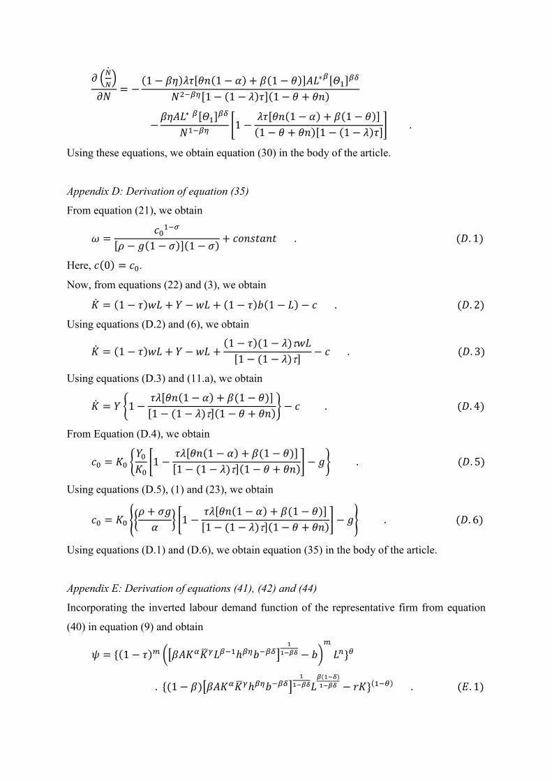
Using these equations, we obtain equation (30) in the body of the article.

Appendix D: Derivation of equation (35)

From equation (21), we obtain

𝜔𝜔 =𝑐𝑐01−𝜎𝜎

[𝜌𝜌 − 𝑔𝑔(1 − 𝜎𝜎)](1 − 𝜎𝜎) + 𝑐𝑐𝑐𝑐𝑛𝑛𝑐𝑐𝑑𝑑𝑎𝑎𝑛𝑛𝑑𝑑 . (𝐷𝐷. 1)

Here, 𝑐𝑐(0) = 𝑐𝑐0.

Now, from equations (22) and (3), we obtain

��𝐾 = (1 − 𝜏𝜏)𝑤𝑤𝑒𝑒 + 𝑌𝑌 − 𝑤𝑤𝑒𝑒 + (1 − 𝜏𝜏)𝑏𝑏(1 − 𝑒𝑒) − 𝑐𝑐 . (𝐷𝐷. 2)

Using equations (D.2) and (6), we obtain

��𝐾 = (1 − 𝜏𝜏)𝑤𝑤𝑒𝑒 + 𝑌𝑌 − 𝑤𝑤𝑒𝑒 +(1 − 𝜏𝜏)(1 − 𝜆𝜆)τ𝑤𝑤𝑒𝑒

[1 − (1 − 𝜆𝜆)τ] − 𝑐𝑐 . (𝐷𝐷. 3)

Using equations (D.3) and (11.a), we obtain

��𝐾 = 𝑌𝑌 �1 −𝜏𝜏𝜆𝜆[𝜃𝜃𝑛𝑛(1 − 𝛼𝛼) + 𝛽𝛽(1 − 𝜃𝜃)]

[1 − (1 − 𝜆𝜆)τ](1 − 𝜃𝜃 + 𝜃𝜃𝑛𝑛)� − 𝑐𝑐 . (𝐷𝐷. 4)

From Equation (D.4), we obtain

𝑐𝑐0 = 𝐾𝐾0 �𝑌𝑌0𝐾𝐾0�1 −

𝜏𝜏𝜆𝜆[𝜃𝜃𝑛𝑛(1 − 𝛼𝛼) + 𝛽𝛽(1 − 𝜃𝜃)][1 − (1 − 𝜆𝜆)τ](1 − 𝜃𝜃 + 𝜃𝜃𝑛𝑛)� − 𝑔𝑔� . (𝐷𝐷. 5)

Using equations (D.5), (1) and (23), we obtain

𝑐𝑐0 = 𝐾𝐾0 ��𝜌𝜌 + 𝜎𝜎𝑔𝑔𝛼𝛼

� �1 −𝜏𝜏𝜆𝜆[𝜃𝜃𝑛𝑛(1 − 𝛼𝛼) + 𝛽𝛽(1 − 𝜃𝜃)]

[1 − (1 − 𝜆𝜆)τ](1 − 𝜃𝜃 + 𝜃𝜃𝑛𝑛)� − 𝑔𝑔� . (𝐷𝐷. 6)

Using equations (D.1) and (D.6), we obtain equation (35) in the body of the article.

Appendix E: Derivation of equations (41), (42) and (44)

Incorporating the inverted labour demand function of the representative firm from equation

(40) in equation (9) and obtain

𝜓𝜓 = {(1 − 𝜏𝜏)𝑚𝑚 ��𝛽𝛽𝐴𝐴𝐾𝐾𝛼𝛼𝐾𝐾�𝛾𝛾𝑒𝑒𝛽𝛽−1ℎ𝛽𝛽𝜂𝜂𝑏𝑏−𝛽𝛽𝛿𝛿�1

1−𝛽𝛽𝛽𝛽 − 𝑏𝑏�𝑚𝑚

𝑒𝑒𝑛𝑛}𝜃𝜃

. {(1− 𝛽𝛽)�𝛽𝛽𝐴𝐴𝐾𝐾𝛼𝛼𝐾𝐾�𝛾𝛾ℎ𝛽𝛽𝜂𝜂𝑏𝑏−𝛽𝛽𝛿𝛿�1

1−𝛽𝛽𝛽𝛽𝑒𝑒𝛽𝛽(1−𝛽𝛽)1−𝛽𝛽𝛽𝛽 − 𝑟𝑟𝐾𝐾}(1−𝜃𝜃) . (𝐸𝐸. 1)

Since equation (40) shows a monotonic relationship between w and L, so we maximise

equation (E.1) with respect to L. Using this first order condition and equation (4), we obtain

𝜃𝜃𝑚𝑚(𝛽𝛽−1)1−𝛽𝛽𝛿𝛿

�𝛽𝛽𝐴𝐴𝐾𝐾𝛼𝛼𝐾𝐾�𝛾𝛾ℎ𝛽𝛽𝜂𝜂𝑏𝑏−𝛽𝛽𝛿𝛿�1

1−𝛽𝛽𝛽𝛽𝑒𝑒𝛽𝛽(1+𝛽𝛽)−21−𝛽𝛽𝛽𝛽

[𝛽𝛽𝐴𝐴𝐾𝐾𝛼𝛼𝐾𝐾�𝛾𝛾𝑒𝑒𝛽𝛽−1ℎ𝛽𝛽𝜂𝜂𝑏𝑏−𝛽𝛽𝛿𝛿]1

1−𝛽𝛽𝛽𝛽 − 𝑏𝑏+𝜃𝜃𝑛𝑛𝑒𝑒

+(1 − 𝜃𝜃)(1 − 𝛽𝛽)�𝛽𝛽𝛽𝛽𝛿𝛿𝐴𝐴𝐾𝐾𝛼𝛼𝐾𝐾�𝛾𝛾ℎ𝛽𝛽𝜂𝜂𝑏𝑏−𝛽𝛽𝛿𝛿�

11−𝛽𝛽𝛽𝛽 𝛽𝛽(1−𝛿𝛿)

1−𝛽𝛽𝛿𝛿𝑒𝑒𝛽𝛽−11−𝛽𝛽𝛽𝛽

(1 − 𝛼𝛼 − 𝛽𝛽)[𝛽𝛽𝛽𝛽𝛿𝛿𝐴𝐴𝐾𝐾𝛼𝛼𝐾𝐾�𝛾𝛾ℎ𝛽𝛽𝜂𝜂𝑏𝑏−𝛽𝛽𝛿𝛿]1

1−𝛽𝛽𝛽𝛽𝑒𝑒𝛽𝛽(1−𝛽𝛽)1−𝛽𝛽𝛽𝛽

= 0 . (𝐸𝐸. 2)

From equation (6), we have

𝑏𝑏 =(1 − 𝜆𝜆)𝜏𝜏𝑤𝑤𝑒𝑒

[1 − (1 − 𝜆𝜆)𝜏𝜏](1− 𝑒𝑒) . (𝐸𝐸. 3)

Now, using equations (40) and (E.3), we obtain

𝑏𝑏 =(1 − 𝜆𝜆)𝜏𝜏�𝛽𝛽𝐴𝐴𝐾𝐾𝛼𝛼𝐾𝐾�𝛾𝛾𝑒𝑒𝛽𝛽(1−𝛿𝛿)ℎ𝛽𝛽𝜂𝜂𝑏𝑏−𝛽𝛽𝛿𝛿�

11−𝛽𝛽𝛽𝛽

[1 − (1 − 𝜆𝜆)𝜏𝜏](1− 𝑒𝑒) . (𝐸𝐸. 4)

Using equations (E.2) and (E.4), we obtain the equation (41) in the body of the article. Now,

using equations (E.3) and (41), we obtain the equation (44) in the body of the article. We

obtain the equation (42) of the main article using equations (E.3) and (40).

References

Adjemian, S., Langot, F., & Quintero-Rojas, C. (2010). How do Labor Market Institutions affect the Link between Growth and Unemployment: the case of the European countries. The European Journal of Comparative Economics, 7(2), 347-371.

Agénor, P.-R., & Neanidis, K. C. (2014). Optimal taxation and growth with public goods and costly enforcement. The Journal of International Trade & Economic Development 23(4), 425-454.

Akerlof, G. A. (1982). Labor Contracts as Partial Gift Exchange. The Quarterly Journal of Economics, 97(4), 543-569.

Akerlof, G. A. (1984). Gift exchange and efficiency-wage theory: Four views. The American Economic Review, 74(2), 79-83.

Akerlof, G. A., & Yellen, J. L. (1986). Efficiency wage models of the labor market. New York: Cambridge University Press.

Bandyopadhyay, D., & Basu, P. (2001). Redistributive Tax and Growth in a Model with Discrete Occupational Choice. Australian Economic Papers 40(2), 111–132.

Blankenau, W. F., & Simpson, N. B. (2004). Public education expenditures and growth. Journal of Development Economics 73(2), 583– 605.

Bräuninger, M. (2000a). Unemployment Insurance, Wage Differentials and Unemployment. FinanzArchiv / Public Finance Analysis 57(4), 485-501.

Bräuninger, M. (2000b). Wage Bargaining, Unemployment, and Growth. Journal of Institutional and Theoretical Economics, 156(4), 646-660.

Bräuninger, M. (2005). Social Security, Unemployment, and Growth. International Tax and Public Finance 12(4), 423-434.

Bucci, A. (2008). Population growth in a model of economic growth with human capital accumulation and horizontal R&D. Journal of Macroeconomics 30(3), 1124–1147.

Caballé, J., & Santos, M. S. (1993). On Endogenous Growth with Physical and Human Capital. Journal of Political Economy 101(6), 1042-1067.

Chakraborty, B., & Gupta, M. R. (2009). Human capital, inequality, endogenous growth and educational subsidy: A theoretical analysis. Research in Economics 63(2), 77–90.

Chang, J.-j., Shaw, M.-f., & Lai, C.-c. (2007). A ‘‘Managerial’’ trade union and economic growth. European Economic Review, 51(2), 365-384.

Corsetti, G., & Roubini, N. (1996). Optimal government spending and taxation in endogenous growth models. NBER Working paper 5851.

Crossley, T. F., & Low, H. (2011). Borrowing constraints, the cost of precautionary saving and unemployment insurance. International Tax and Public Finance 18(6), 658-687.

Danthine, J.-P., & Kurmann, A. (2006). Efficiency wages revisited: The internal reference perspective. Economics Letters, 90(2), 278–284.

Davidson, C., & Woodbury, S. A. (1997). Optimal unemployment insurance. Journal of Public Economics 64(3), 359–387.

Docquier, F., Faye, O., & Pestieau, P. (2008). Is migration a good substitute for education subsidies? Journal of Development Economics 86(2), 263–276.

Garino, G., & Martin, C. (2000). Efficiency wages and union–firm bargaining. Economics Letters, 69(2), 181–185.

Glomm, G., & Ravikumar, B. (1997). Productive government expenditures and long-run growth. Journal of Economic Dynamics and Control 21(1), 183–204.

Irmen, A., & Wigger, B. U. (2002/2003). Trade Union Objectives and Economic Growth. FinanzArchiv / Public Finance Analysis, 59(1), 49-67.

Kitaura, K. (2010). Fiscal Policy and Economic Growth in the Imperfect Labor Market. Metroeconomica, 61(4), 686–700.

Lai, C.-H., & Wang, V. (2010). The effects of unionization in an R&D growth model with (In)determinate equilibrium. MPRA Paper 27748. University Library of Munich, Germany.

Landais, C., Michaillat, P., & Saez, E. (2010). Optimal Unemployment Insurance Over the Business Cycle. NBER Working Paper No. 16526.

Lingens, J. (2003a). The impact of a unionised labour market in a Schumpeterian growth model. Labour Economics, 10(1), 91-104.

Lingens, J. (2003b). Unionisation, Growth and Endogenous Skill-Formation. Economics Discussion Papers No. 45/03. University of Kassel, Institute of Economics, Germany.

Lucas Jr., R. E. (1988). On the mechanics of economic development. Journal of Monetary Economics 22(1), 3–42.

Marti, C. (1997). Efficiency wages: combining the shirking and turnover cost models. Economics Letters, 57(3), 327–330.

Mauleon, A., & Vannetelbosch, V. J. (2003). Efficiency wages and union-firm bargaining with private information. Spanish Economic Review, 5(4), 307-316.

McDonald, I. M., & Solow, R. M. (1981). Wage Bargaining and Employment. The American Economic Review, 71(5), 896-908.

Ni, S., & Wang, X. (1994). Human capital and income taxation in an endogenous growth model. Journal of Macroeconomics, 16(3), 493–507.

Nickell, S. J., & Andrews, M. (1983). Unions, Real Wages and Employment in Britain 1951-79. Oxford Economic Papers, New Series, 35, 183-206.

Palokangas, T. (1996). Endogenous growth and collective bargaining. Journal of Economic Dynamics and Control, 20(5), 925-944.

Palokangas, T. (2003). Labour Market Regulation, Productivity-Improving R&D and Endogenous Growth. IZA Discussion Papers no. 720.

Palokangas, T. (2004). Union–Firm Bargaining, Productivity Improvement and Endogenous Growth. LABOUR, 18(2), 191–205.

Peach, E. K., & Stanley, T. D. (2009). Efficiency Wages, Productivity and Simultaneity: A Meta-Regression Analysis. Journal of Labor Research, 30(3), 262-268.

Pereau, J., & Sanz, N. (2006). Trade unions, efficiency wages and employment. Economics Bulletin, 10(4), 1−8.

Ramos Parreño, J. M., & Sánchez-Losada, F. (2002). The role of unions in an endogenous growth model with human capital. Journal of Macroeconomics, 24(2), 171–192.

Raurich, X., & Sorolla, V. (2003). Growth, unemployment and public capital. Spanish Economic Review, 5(1), 49-61.

Romer, D. (2006). Advanced macroeconomics. New York: McGraw-Hill / Irwin. Shapiro, C., & Stiglitz, J. E. (1984). Equilibrium Unemployment as a Worker Discipline

Device. The American Economic Review, 74(3), 433-444. Solow, R. M. (1979). Another possible source of wage stickiness. Journal of

Macroeconomics, 1(1), 79–82. Sorensen, J. R. (1997). Do Trade Unions Actually Worsen Economic Performance? Working

Paper No. 1997-6. School of Economics and Management, University of Aarhus. Stiglitz, J. E. (1976). The Efficiency Wage Hypothesis, Surplus Labour, and the Distribution

of Income in L.D.C.s. Oxford Economic Papers, 28(2), 185-207. Tournemaine, F., & Tsoukis, C. (Forthcoming). Public Expenditures, Growth and

Distribution in a Mixed Regime of Education with a Status Motive. Journal of Public Economic Theory.

Uzawa, H. (1965). Optimum Technical Change in An Aggregative Model of Economic Growth. International Economic Review 6(1), 18-31.

Yellen, J. L. (1984). Efficiency Wage Models of Unemployment. The American Economic Review, 74(2), 200-205.

Chandril Bhattacharyya

Economic Research Unit, Indian Statistical Institute,

203, B.T. Road, Kolkata 700 108, India.

E-mail address: chandrilbhattacharyya@gmail.com

Manash Ranjan Gupta

Economic Research Unit, Indian Statistical Institute,

203, B.T. Road, Kolkata 700 108, India.

E-mail address: manashgupta@isical.ac.in