MPRAMunich Personal RePEc Archive

Estimating Urban AgglomerationEconomies for India: A New EconomicGeography Perspective

Sabyasachi Tripathi

December 2012

Online at https://mpra.ub.uni-muenchen.de/43501/MPRA Paper No. 43501, posted 31. December 2012 14:29 UTC

1

Estimating Urban Agglomeration Economies for India: A

New Economic Geography Perspective

Sabyasachi Tripathi*

Abstract: The main objective of this paper is to provide answer to an important question:

Are Indian firms or industries in urban areas operating under decreasing returns to scale or

increasing returns to scale? Scale economies are one of the main assumptions of new

economic geography models that posit the formation of agglomeration economies. For this

purpose, we use Kanemoto et al. (1996) model for estimation of aggregate production

function and to derive the magnitude of scale economies. Using firm level data in 2004-05

from the Annual Survey of Industry, we find that urban firms in Indian industry operate under

decreasing returns to scale.

JEL classification: F23; R0

Keywords: Economic geography, Urban agglomeration, Firm level analysis, Manufacturing

industry, India.

Acknowledgement:

This paper is the part of my Doctoral Dissertation. I would like to thank my Ph.D., thesis

supervisor Prof. M.R.Narayana for his constant guidance, inspiration, valuable comments and

suggestions. I thank Prof. Arne Melchior, Dr. Jagnnath Mallick, Prof. Meenakshi Rajeeb,

Prof. Rupa Cahanda, Dr. Krishna raj and Somnath Das for their very helpful comments and

discussion. I also would like to thank Dr. Giulio Bottazzi and other participants of the

DIMETIC Session 2 (July 2010) from the Department of Economics and Regional Studies-

Faculty of Business and Economics- University of Pecs, for constructive suggestions. Finally,

I place on record my grateful thanks to Dr. Soumya Chakraborty from Central Statistical

Office for helping me to comprehend the data and for providing me valuable clues on

judicious data-use. However, the usual disclaimer applies.

*Ph.D. Scholar in Economics, Institute for Social and Economic Change, Bangalore –

560072. Email: sabya.tripathi@gmail.com

2

1. Introduction

In contemporary economic studies, theoretical models of “New Economic geography”

(pioneered by Krugman, 1991), have been found to be the most successful in explaining the

uneven allocation of economic activity across space, principally due to its emphasis on the

“second nature geography” (i.e., the distance of the economic agents relative to one another

in space). Previous studies of neoclassical economies, particularly on the issue of distribution

of economic activity, were based on “first-nature geography” (i.e., endowment of resources,

the physical geography of climate, and topology). The core assumptions of new economic

geography (hereafter, NEG) are product differentiations such as, a) modeled through a love

of variety assumption, b) increasing returns to scale at firm level (so that firms have an

incentive to produce in one place) and c) reduction of transport costs (so that it matters where

you produce). These assumptions together create pecuniary externalities in agents‟ location

choice (Redding, 2010) and also guide the forces of cumulative causation and agglomeration

with the aid of mixed factor mobility or tradable intermediate inputs. However, unlike the

earlier location theories, the NEG comprises of a general equilibrium framework with

imperfect competition.

Several academics (such as, Marshal, 1890; Weber, 1909; Hotelling, 1929; Lösch, 1940;

Isard, 1956; Greenhut and Greenhut, 1975; for an excellent review, see Ottaviano and Thisse,

2005) have in the past dealt with agglomeration economics, i.e., examination of the location

and geographic concentration of economic activity. But, of the stress on increasing returns for

agglomeration economics mainly came from the Starrett‟s (1978) „Spatial Impossibility

Theorem‟.1

Indian studies on industrialization related urban agglomeration include the following:

Chakravorty et al. (2005) use the disaggregated industry location and size data from Mumbai,

Kolkata, and Chennai, to analyze eight industrial sectors. Their indicative results suggest that

general urbanization economies are more important than localization economies for firm‟s

location decisions. Lall et al. (2004) suggest that the access to market through -

1 The theorem states that if space is homogeneous (i.e., each region is same in terms of consumer preferences,

endowments and firm‟s production possibilities) and transportation is costly, there does not exist a competitive

equilibrium involving goods being traded between regions. Perfect competition combined with transport costs

and homogeneous space would produce at small scale or each region will produce for itself (i.e., so-called

backyard capitalism) [see Ottaviano and Thisse, 2004, for detailed discussion]. Therefore, substantial

localization or spatial concentration of economic activity may be seen as sign of agglomeration economies

(Puga, 2010).

3

improvements in inter-regional infrastructure is an important determinant of firm level

productivity, whereas benefits of locating in dense urban areas do not offset associated costs.

Lall and Mengistae (2005a) find that both the local business environment and agglomeration

economies significantly influence business location choices across Indian cities. Lall and

Mengistae (2005b) study at plant level from India‟s major industrial centers shows large

productivity gaps across cities due to differences in agglomeration economies, degree of

labor regulation, severity of power shortages, and market access. Lall et al. (2003) find that

generalized urbanization economies (manifested in local economic diversity) provide the

agglomeration externalities that lead to industrial clustering in metropolitan and other India‟s

urban areas. Chakravorty‟s (2003) findings provide evidence both of inter-regional

divergence and intra-regional convergence, and suggest that „concentrated decentralization‟ is

the appropriate framework for understanding industrial location in post-reform India. Lall and

Chakravorty (2005) examine the contribution of economic geography factors to the cost

structure of firms in eight industry sectors and show that local industrial diversity is an

important factor with significant and substantial cost-reducing effects. Mukherjee (2008)

finds evidence to support the hypothesis that the trade liberalization of 1991 has resulted in

agglomeration based on increasing returns in India, and four industries, namely, Iron and

Steel, Chemical, Textile and Non-electrical have experienced some locational shifts after the

trade liberalization.

Other studies identify various causative factors for firm location choice. These are abundant

power (Rajaraman, et al., 1999); power availability (rather than its price), reliable

infrastructure and factors of production (Mani, et al., 1996); sales tax incentive (Tulasidhar

and Rao, 1986); and labour regulation (Besley and Burgess, 2004 and Lall and Mengistae,

2005b). Sridhar and Wan (2010), using the World Bank‟s Investment Climate Survey (ICS)

data for India, find that more labour-intensive firms tend to refrain from locating in medium-

sized cities relative to smaller cities in India and that Indian firms find capital cities

attractive. This reinforces that public investments are biased in favour of capitals where

policy makers live (Henderson, et al., 2000). In addition, they find that firm efficiency has a

significant positive impact on the log odds of a firm locating in the large cities of India.

Sridhar (2005) argues that infrastructure, power, telecom, roads and banking are important

determinants of firm location in the growth centres of India. Fernandes and Sharma (2012)

find that large plants led to lower spatial concentration and FDI liberalization and de-

4

licensing caused small plants to disperse while trade liberalization had the opposite effect.

Most importantly, Ghani et al. (2012) find that plants in the formal sector are moving away

from urban and into rural locations, while the informal sector is moving from rural to urban

locations and the secular trend in India‟s manufacturing urbanization has slowed down.

There are few international studies on urban agglomeration that includes India as well.

Investment Climate and Manufacturing Industry report (2004) by World Bank shows that the

two main factors affect the individual firm‟s location decision. First, “business environment”

includes access to inputs (quality and cost of labor and capital); access to markets; provision

of basic infrastructure; institutional environment; and industry-specific subsidies or tax

breaks. Second, “agglomeration economies” increase returns to scale.

In essence, the above cited review of an exhaustive collection of Indian studies identifies the

relevant determinants of firm locational choice, and the different levels of productivity a firm

experiences when it operates in Indian cities or towns. In this perspective, in line with the

prediction of NEG models, the main focus of this paper is to estimate the firm or industry

level economies of scale which drives agglomeration economies in the absence of

technological externalities as also when accompanied by significant market failure (Fujita et

al. 2004). More specifically, we examine the following question in this paper: whether Indian

firms or industry in urban areas (or in cities) are operating under the decreasing returns to

scale or increasing returns to scale. Using the firm level data 2004-05 from the Annual

Survey of Industry, our main finding is that urban firms in Indian industry operate under the

decreasing returns to scale, which offers no evidence of increasing returns to scale for

agglomeration economics as predicted in the NEG models. .

The organization of this paper is as follows. In section 2, we have described the basic

framework of the new economic geography. In section 3 and 4, we explain the aggregate

production functions for metropolitan areas in order to estimate the agglomeration

economies. In section 5, we summarize the results, and in section 6 we discuss possibilities

for elaboration and extension.

5

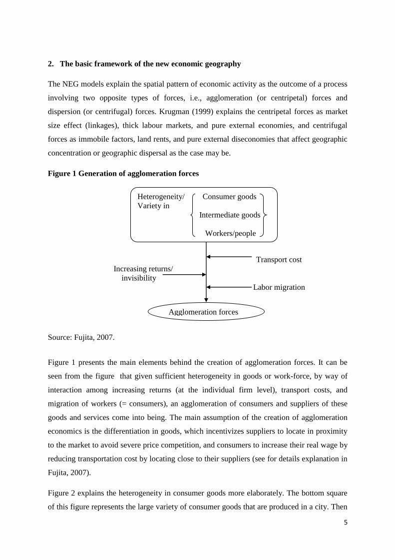
2. The basic framework of the new economic geography

The NEG models explain the spatial pattern of economic activity as the outcome of a process

involving two opposite types of forces, i.e., agglomeration (or centripetal) forces and

dispersion (or centrifugal) forces. Krugman (1999) explains the centripetal forces as market

size effect (linkages), thick labour markets, and pure external economies, and centrifugal

forces as immobile factors, land rents, and pure external diseconomies that affect geographic

concentration or geographic dispersal as the case may be.

Figure 1 Generation of agglomeration forces

Transport cost

Increasing returns/

invisibility

Labor migration

Source: Fujita, 2007.

Figure 1 presents the main elements behind the creation of agglomeration forces. It can be

seen from the figure that given sufficient heterogeneity in goods or work-force, by way of

interaction among increasing returns (at the individual firm level), transport costs, and

migration of workers (= consumers), an agglomeration of consumers and suppliers of these

goods and services come into being. The main assumption of the creation of agglomeration

economics is the differentiation in goods, which incentivizes suppliers to locate in proximity

to the market to avoid severe price competition, and consumers to increase their real wage by

reducing transportation cost by locating close to their suppliers (see for details explanation in

Fujita, 2007).

Figure 2 explains the heterogeneity in consumer goods more elaborately. The bottom square

of this figure represents the large variety of consumer goods that are produced in a city. Then

Heterogeneity/ Consumer goods

Variety in

Intermediate goods

Workers/people

Agglomeration forces

6

given a nominal wage in the city, with the love of verity assumption (or taste of variety), the

real income of workers tends to rise as they purchase goods at lower prices in the city in

preference to more distance places. This leads to migration of consumers (= workers) and

increases the demand of goods in the city. Furthermore, due to home market effect (i.e., the

benefits of locating near a large market) more specialized firms will emerge and produce

Figure 2: Circular causality in spatial agglomeration of consumer-goods

producers and workers (= consumers).

Backward Forward

linkages linkages

Source: Fujita, 2007.

a new variety of goods in the city. Thus, through the forward linkages (the supply of greater

variety of goods increases the workers‟ real income) and backward linkages (a greater

number of consumers attract more firms) the agglomeration of firms and workers in the city

occurs. Finally, through these linkages, pecuniary externalities occur, scale economies (at the

firm level) emerge and increasing returns occur at the city level (see for more details

explanation Fujita, 2007).

The above explanation shows that the circular causation leading to agglomeration economies

depends mainly on scale economies in the form of increasing returns to scale. For that reason,

More consumers (=

workers) locate in the

city

A greater number

of specialized firms

can be supported

Higher real income

from a given nominal

wage

More variety of

consumer goods

produced in a city

Test for

variety

Scale

economies in

specialized

production

7

the measurement of scale economies at firm levels in urban industry is important, and hence

constitutes the main focus of this paper.

3. Theoretical frame work

We estimate an aggregate production function for urban India to derive estimates of the

nature and magnitude of urban agglomeration economies. For this purpose we use Kanemoto,

et al. (1996) model. The model is also used by Fujita, et al. (2004) and Kanemoto, et al.

(2005). The significance of using this model is that it considers the traditional production

function by incorporating the assumption of NEG models (i.e., increasing labour force in a

large agglomeration leads to higher production of city output) to estimate the economies of

scale for firms (or industry) level.

An aggregate neoclassical production function for a city (or urban area) is given by:

Y = F (N,K,G,M) ------------------ (1)

where N,K,G, M and Y are respectively employment, the private capital, social overhead

capital, materials and the total production in an urban area. All the factors of production are

finite and non-negative. The importance of introducing the social overhead capital for

measuring agglomeration economics has been established by many researchers (see Fujita et

al. 2004, for a review). The main assumption is that, in the absence of agglomeration

economies, the production function exhibits constant returns to scale with respect to labor and

capital inputs. Therefore, the degree of agglomeration economies can be measured by the

degree of increasing returns to scale of the estimated production function.

To capture the non-market interaction between firms combined with transportation and

communication costs (i.e., heterogeneity of final and/or intermediate goods combined with

transportation cost), we use the following Cobb-Douglas production function in the form of

structural equation [Kanemoto, 1990 and Krugman, 1991].2

2 Original model of Kanemoto, et al., (1996) used the following different Cobb-Douglas production functions to

estimate the agglomeration economics for Japan:

𝑌 = 𝐴𝐾𝛼𝑁𝛽𝐺𝛾 ------ (i) 𝑌 = 𝐴𝐾𝛼𝑁1−𝛼𝑁𝛾𝑙𝑛𝐺 ----- (ii)

The specification of equation (2) is used in case of India, as it provides the best results in terms of measuring

positive agglomeration economies for organized manufacturing firms (or industries).

8

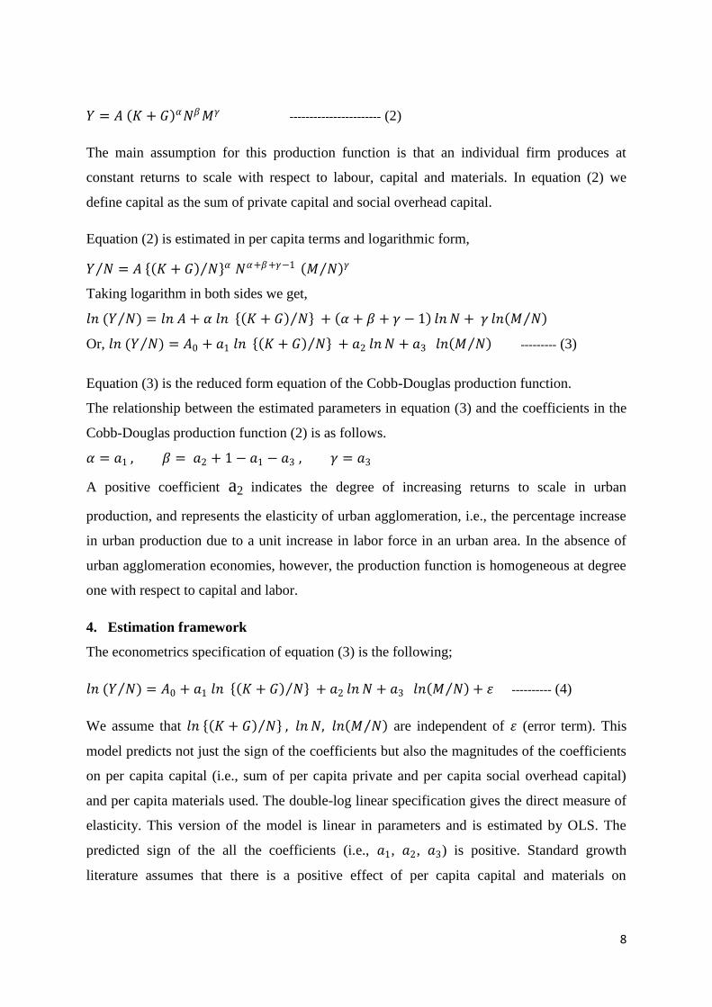
𝑌 = 𝐴 𝐾 + 𝐺 𝛼𝑁𝛽𝑀𝛾 ----------------------- (2)

The main assumption for this production function is that an individual firm produces at

constant returns to scale with respect to labour, capital and materials. In equation (2) we

define capital as the sum of private capital and social overhead capital.

Equation (2) is estimated in per capita terms and logarithmic form,

𝑌 𝑁 = 𝐴 𝐾 + 𝐺 𝑁 𝛼 𝑁𝛼+𝛽+𝛾−1 𝑀 𝑁 𝛾

Taking logarithm in both sides we get,

𝑙𝑛 (𝑌 𝑁) = 𝑙𝑛 𝐴 + 𝛼 𝑙𝑛 𝐾 + 𝐺 𝑁 + 𝛼 + 𝛽 + 𝛾 − 1 𝑙𝑛𝑁 + 𝛾 𝑙𝑛 𝑀 𝑁

Or, 𝑙𝑛 (𝑌 𝑁) = 𝐴0 + 𝑎1 𝑙𝑛 𝐾 + 𝐺 𝑁 + 𝑎2 𝑙𝑛𝑁 + 𝑎3 𝑙𝑛 𝑀 𝑁 --------- (3)

Equation (3) is the reduced form equation of the Cobb-Douglas production function.

The relationship between the estimated parameters in equation (3) and the coefficients in the

Cobb-Douglas production function (2) is as follows.

𝛼 = 𝑎1 , 𝛽 = 𝑎2 + 1 − 𝑎1 − 𝑎3 , 𝛾 = 𝑎3

A positive coefficient a2 indicates the degree of increasing returns to scale in urban

production, and represents the elasticity of urban agglomeration, i.e., the percentage increase

in urban production due to a unit increase in labor force in an urban area. In the absence of

urban agglomeration economies, however, the production function is homogeneous at degree

one with respect to capital and labor.

4. Estimation framework

The econometrics specification of equation (3) is the following;

𝑙𝑛 (𝑌 𝑁) = 𝐴0 + 𝑎1 𝑙𝑛 𝐾 + 𝐺 𝑁 + 𝑎2 𝑙𝑛 𝑁 + 𝑎3 𝑙𝑛 𝑀 𝑁 + 𝜀 ---------- (4)

We assume that 𝑙𝑛 𝐾 + 𝐺 𝑁 , 𝑙𝑛 𝑁, 𝑙𝑛 𝑀 𝑁 are independent of 𝜀 (error term). This

model predicts not just the sign of the coefficients but also the magnitudes of the coefficients

on per capita capital (i.e., sum of per capita private and per capita social overhead capital)

and per capita materials used. The double-log linear specification gives the direct measure of

elasticity. This version of the model is linear in parameters and is estimated by OLS. The

predicted sign of the all the coefficients (i.e., 𝑎1, 𝑎2, 𝑎3) is positive. Standard growth

literature assumes that there is a positive effect of per capita capital and materials on

9

production. Finally, following the literature of NEG models the positive value of 𝑎2 (i.e.,

increasing returns to scale) is predicted.

4.1 Measurement of variables and data sources

We have used the firm level data in 2004-05 from Annual Survey of Industries (ASI),

conducted by the Central Statistical Office (CSO) of the Government of India.3

Data on

output, employees, private capital, and materials are used in the estimation (Table 1).

Table 1: Firm level variables used in the study

Variables Description (as definitions are given by ASI)

Output Factory value of products and by-products manufactured as well as

other receipts from non industrial services rendered to others, work

done for others on material supplied by them, value of electricity

produced and sold, sale value of goods sold in the same conditions

purchased, addition in stock of semi- finished goods and value of

own construction.

Private

Capital

Private capital is the sum of total value/ depreciated value of fixed

assets owned by the factory as on the closing day of the accounting

year. Fixed assets are those that have a normal productive life of

more than one year. Fixed capital includes land including lease- hold

land, buildings, plant and machinery, furniture and fixtures, transport

equipment, water system and roadways and other fixed assets such

as hospitals, schools etc. used for the benefit of factory personnel.

Labour Total man-day employees, which is the total number of days worked

and the number of days paid for during the accounting year. It is

obtained by summing-up the number of persons of specified

categories attending in each shift over all the shifts worked on all

days.

Materials Material input for each firm is defined as the total delivered value of

all items of raw materials, components, chemicals, packing materials

and stores, that has actually entered into the production process of

the factory during the accounting year. This includes the cost of all

materials used in the production process of the factory during the

accounting year as also the cost of all materials used in the

production of fixed assets including construction work for factory‟s

own use.

Source: Author’s compilation

3 The ASI covers factories registered under sections 2m(i) and 2m(ii) of the factories Act 1948, employing 10 or

more workers and using power, and those employing 20 or more workers but not using power on any day of the

preceding 12 months.

10

Following Lall et al. (2004), we consider the total output as production of a firm, and total

man-day employees are used as a proxy of labour. Most specifically, we define production

function excluding intermediate consumption. Therefore, total output is considered as a

measure of output than gross value added. In addition, private capital and materials are used

as important variables in the estimation of firm level production function. Doms (1992)

argues that defining capital as a gross stock is a reasonable approximation for capital. For that

reason, our measurement of private capital (and in the ASI dataset) is defined as the gross

value of plant and machinery. It also includes the book value of installed plant and machinery

and the approximate value of rented-in plant and machinery. We also measure material as per

the definition of ASI.

The geographic attributes allows us to identify each firm at the state level (or district level)

with rural urban distinction.4 Available information allows us to categorize firms by their

location in urban areas of a state (or district) as well as the total urban area in the country, but

not in any specific urban centre.5 The analysis is carried out for 25 states

in India for the

entire industry sector at five-digit National Industry Classification (NIC) codes of 2004.6,7

For our analysis we have considered all types of ownership of the firm, which includes

wholly central government, wholly state and/or local government, central government and

state and/or local government jointly, joint sector public, joint sector private, and wholly

private ownership. This also includes those firms that are using foreign direct investment

(FDI) for production. This is very important because FDI flow is one of the main factors

behind firm location choice for different regions as well as different states.

4

The ASI data allows the identification of the firms at the state level with rural-urban distinction, but these data

are not made available for district level due to confidentially concern. However, on special request, CSO has

provided information only for some large city districts which is used in this study. 5

Population Census of India categorizes urban centres into six based on population size. Class I (100,000 or

more), Class II (from 50,000 to 99,999), Class III (from 20,000 to 49,999), Class IV (from 10,000 to 19,999),

Class V (from 5000 to 9999) and Class VI (below 5000) 6

Although in India there are 35 states (including Union Territories), we consider 25 of them due to non-

availability of information or due to very small number of observations. 7 National Industry Classification (NIC) codes of 2004 do not include India‟s best known “industrial” export-

software (which embodies high levels of human capital) in the data.

11

4.1.1 Measurement of Social overhead capital

Construction of Social overhead capital variable at firm level is described here. Kenemoto,

Ohkawara and Suzuki (1996) have defined social overhead capital by allocating industrial

infrastructure investment with capital stock in telecommunication and railway industries. Aso

(2008), in the study “Social overhead capital development and geographical concentration”

have used traffic infrastructure investment which includes railroad, automobile, ship and

airplane. In the Indian context, data for the above variables are not available for urban areas

at state level as well as for district (or city) level.

For that reason, firm level share of public Net Fixed Capital Stock (NFCS) is used as proxy

of Industry (or firm) level social overhead capital. Public NFCS comprises administrative

departments, departmental commercial undertakings (DCUs) and non-departmental

commercial undertakings (NDCUs). The social overhead capital expenditure includes mainly

the physical infrastructure which is dominated by the public sector. Therefore, the public

NFCS is used as proxy to measure the Social overhead capital. However, firm level NFCS is

estimated by allocating the state (or district) wise urban share of NFCS, multiplied by the

ratio of a firm‟s expenditure on electricity consumption to the total expenditure on electricity

by all the firms operating in an urban area (i.e., state or district).8,9

i.e., 𝑁𝐹𝐶𝑆𝑗𝑘 = 𝐸𝑗𝑘

𝐸𝑗𝑘𝑗 × 𝑁𝐹𝐶𝑆𝑖

𝑃,𝑈 ------------ (5)

Where 𝑁𝐹𝐶𝑆𝑗𝑘 stands as urban share of Public NFCS value of 𝑗th firm operating in 𝑘th

urban (which may be state or district) area, 𝐸𝑗𝑘 stands as total expenditure on electricity by

𝑗th firm operating in 𝑘th urban (which may be state or district) area. 𝐸𝑗𝑘𝑗 stands as total

expenditure on electricity by all the firms operating in 𝑘th urban (which may be state or

district) area. 𝑁𝐹𝐶𝑆𝑖𝑃,𝑈

stands as public (denoted by P) urban (denoted by U) NFCS value of

𝑖th state (or district).

8 For the measurement of social overhead capital for firm level, initially, we allocated total urban public NFCS

with the share of individual firm‟s private capital stock to total private capital stock by all the urban firms in a

state (or by the ratio of individual firm‟s output to total output by all the urban firms in a state). Then we

encountered the problem of multicolliearity, as correlation coefficients between private capital (or firm‟s output)

and social overhead capital were unity. For that reason we have considered firm‟s electricity expenditure data

for allocation of state public capital. 9

The firm‟s expenditure on electricity which is considered as output of public sector is used as input of a firm‟s

production function. This is typically a Leontief case of input-output model (i.e., how the output of one industry

is an input to each other industry). However, as input output data are available only at sector level and not at any

industry (or firm) specific level, we do not construct (or analyze) input-output model.

12

Total NFCS in public sector is available only at the national level. The public NFCS in 2005

is Rs. 2909398 (Crore) at current prices as given in CSO (2008). We take the value of public

NFCS at current prices as in the case of other variables (such as public sector Gross Fixed

Capital Formation (GFCF) is only available in current prices).

For the calculation of public urban NFCS value of a state (or district), following two steps are

considered:

Step 1: Estimation of state (or district) wise total public NFCS:

To estimate the state level NFCS, we multiply the value of national level NFCS with the ratio

of state level GFCS share. i.e.,

𝑁𝐹𝐶𝑆𝑖𝑃 =

𝐺𝐹𝐶𝐹𝑖𝑃

𝐺𝐹𝐶𝐹𝑖𝑃

𝑖× 𝑁𝐹𝐶𝑆𝑃 -------------------- (6)

Where 𝑁𝐹𝐶𝑆𝑖𝑃 stands as public NFCS of 𝑖th state (or Union Territory), 𝐺𝐹𝐶𝐹𝑖

𝑃refers to total

public sector GFCF value of the 𝑖th state, 𝐺𝐹𝐶𝐹𝑖𝑃

𝑖 stands as total public sector GFCF of all

the states (or Union Territory) of India, and 𝑁𝐹𝐶𝑆𝑃 refers to total national level public

NFCS. We also add expenditure on Supra-regional expenditure in calculation of total public

GFCF as Supra-regional sectors include railways, banking and insurance, communications

and central Government administration (see Table 2 for details).

Social overhead capital is a stock concept. As long time series data on state level public

GFCF are not available, we could not measure the capital stock using perpetual inventory

method (PIM). Therefore, the national public NFCS is distributed on the basis of share of

state level GFCF.

Step 2: Estimation of state (or district) wise total public urban NFCS:

For state level: We allocate state wise total public NFCS with share of national level urban

NDP, i.e.,

𝑁𝐹𝐶𝑆𝑖𝑃,𝑈 =

𝑁𝐷𝑃𝑢

𝑁𝐷𝑃× 𝑁𝐹𝐶𝑆𝑖

𝑃 --------------------- (7)

Where NDP stands as All India level Net Domestic Product, 𝑁𝐷𝑃𝑢 refers to the urban NDP.

Total public sector GFCF for 2004-05 was collected from the report of Government of India

(GOI, 2009). NDP of urban area for the year 2004-05 was collected from CSO (2010). The

13

NDP for total urban areas in current prices is Rs. 1376653(Crore) and for total rural areas is

Rs. 1269717 (Crore). Total urban NDP as percentage of total is 0.52.

At the district level: We allocate state wise total public NFCS with share of district level

DDP to state level total GSDP. i.e.,

𝑁𝐹𝐶𝑆𝑖𝑃,𝑈 =

𝐺𝐷𝐷𝑃 𝑖

𝐺𝑆𝐷𝑃 𝑖× 𝑁𝐹𝐶𝑆𝑖

𝑃 --------------------- (8)

Where 𝐺𝐷𝐷𝑃𝑖 stands as Gross District Domestic Product of a particular district in which the

sample city is located, 𝐺𝑆𝐷𝑃𝑖 refers to the Gross State Domestic Product of a particular state

in which the district is located. We consider GSDP and GDDP, as city output and state level

rural urban distinction GSDP are not available.

4.1.2 Importance of using social overhead capital as one of the explanatory variables

Regional connectivity is determined by the status of transport infrastructure, and market

access increases with increase in regional connectivity. By lowering transportation cost of

output and input, transport infrastructure increases real income (even if the price of the

commodity remains same) of the workers and also consumer surplus leading to increase in

productivity. It also increases interaction and spillovers between firms, firms and research

centers, government and regulatory institutions, etc. Therefore, improvements of transport

network increases the potential size of agglomeration by attracting private investment (see

Lall et al., 2004 for more details)

To construct the social overhead capital, we have used public GFCF which includes two

types of fixed assets, namely construction (buildings) and machinery and equipment which in

turn include transport equipment, software and breeding stock, draught animals, dairy cattle,

etc. Construction activity covers all new constructions and major alternations and repairs of

buildings, highways, streets, bridges, culverts, railroad beds, subways, airports, parking area,

dams, drainages, wells and other irrigation sources, water and power projects, communication

systems such as telephone and telegraph lines, land reclamations, bunding and other land

improvements, afforestation projects, installation of wind energy system etc. Machinery and

equipments comprise all types of machineries like agricultural machinery, power generating

machinery, manufacturing, transport equipment, furniture and furnishing.

14

Table 2: Estimation of state wise urban share of Public Net Fixed Capital Stock (NFCS)

Sr.

No.

Name of the

States

Public GFCF (Rs. Crores)

GFCF

Share

Total

Public

NFCS (Rs.

Crore)

Total Public

Urban NFCS

(Rs. Crore)

Public

sector

Total

Supra

Regional Total

1 Andhra Pradesh 11219 1456 12675 0.0629 182961 95140

2 Arunachal Pradesh 1962 66 2028 0.0101 29274 15222

3 Assam 6636 346 6982 0.0346 100783 52407

4 Bihar 4858 1157 6015 0.0298 86825 45149

5 Chhattisgarh 4503 473 4976 0.0247 71827 37350

6 Goa 718 81 799 0.0040 11533 5997

7 Gujrat 12498 1160 13658 0.0678 197150 102518

8 Haryana 5659 376 6035 0.0299 87114 45299

9 Himachal Pradesh 3537 168 3705 0.0184 53481 27810

10 Jharkhand 2746 1628 4374 0.0217 63138 32832

11 Jammu & Kashmir 5051 556 5607 0.0278 80936 42087

12 Karnataka 10307 1626 11933 0.0592 172250 89570

13 Kerala 3603 900 4503 0.0223 65000 33800

14 Madhya Pradesh 10434 760 11194 0.0555 161583 84023

15 Maharashtra 20866 2970 23836 0.1183 344067 178915

16 Manipur 1136 63 1199 0.0059 17307 9000

17 Meghalaya 716 63 779 0.0039 11245 5847

18 Mizoram 2002 51 2053 0.0102 29635 15410

19 Nagaland 1048 67 1115 0.0055 16095 8369

20 Orissa 5424 715 6139 0.0305 88615 46080

21 Punjab 3073 999 4072 0.0202 58778 30565

22 Rajasthan 5659 954 6613 0.0328 95457 49638

23 Sikkim 1377 13 1390 0.0069 20064 10433

24 Tamil Nadu 13103 1444 14547 0.0722 209982 109191

25 Tripura 963 78 1041 0.0052 15027 7814

26 Uttar Pradesh 15579 1951 17530 0.0870 253041 131581

27 Uttarkhand 4775 202 4977 0.0247 71842 37358

28 West Bengal 9592 1732 11324 0.0562 163459 84999

29 Andaman & N.I. 198 39 237 0.0012 3421 1779

30 Chandigarh 175 78 253 0.0013 3652 1899

31 Dadra & Nagar H. 35 1 36 0.0002 520 270

32 Daman & Diu 12 2 14 0.0001 202 105

33 Delhi 5526 3933 9459 0.0469 136538 71000

34 Lashadweep 391 2 393 0.0019 5673 2950

35 Punducherry 49 15 64 0.0003 924 480

Total 175430 26125 201555 1 2909398 1512887

Source: GOI (2009) and Author’s calculation.

15

For that reason Social Overhead Capital is taken as a proxy of transport infrastructure

investment, because urban agglomeration depends on scale economies associated with

reduction in transportation cost. For obvious reasons, the trade-off between increasing

returns and transport costs is fundamental to the understanding of the geography of economic

activities.

4.1.3 Description of Data

A total of 60825 firms are considered for the entire analysis by five main variables, namely,

output, labour, private capital, social overhead capital, and materials. Table 3 gives the

descriptive statistics of the five variables. It shows that mean of output, social overhead

capital, private capital, and materials is Rs. 456000000, Rs. 753000000, Rs. 147000000, and

Rs. 262000000 respectively. Mean labour is 61003. The coefficient of variation of output,

labour, social overhead capital, private capital and materials is 999, 211, 1173, 1312, and

808, respectively. As the coefficient of variation is a pure number and highest (or lowest) for

private capital (or labour), it can be said that the relative variability is highest (or lowest) in

data on private capital (or labour) then the other variables. The positive skewness values for

all the variables indicate that the distribution is right-skewed or right-tailed, which means the

values of the variables tend to cluster to the lower end of the scale (i.e., smaller number) with

increasingly fewer values of the variables at the upper end of the scale (i.e., the large

numbers). In addition, positive kurtosis for all the variables indicates heavy tails and

peakedness relative to the normal distribution.

Table 3: Descriptive Statistics: All India Urban Firms

Variables

Mean

(in

Millions)

Std. Dev.

(in

Millions)

Mini-

mum

Maximum

(in

Billions)

Ske

w-

ness

Kurto-

sis

Coefficient

of

Variation

Output(Rs.) 456 4550 42 436 58 4624 999

Labour 0.061 0.129 30 0.005 11 222 211

Social

overhead

Capital(Rs.) 753 8830 7114 846 70 5912 1173

Private

capital(Rs.) 147 1930 158 214 74 7617 1312

Materials 262 2120 493 162 45 2643 808

Source: Author‟s calculation

16

5. Estimation Result

5.1 All India level analysis for all the firm together: Urban

The coefficient a2 (=α+β+γ-1) in equation (4) measures the economies of scale in urban

production. The sign and value of this coefficient explains whether the urban firms in Indian

industry operate under increasing returns to scale or decreasing returns to scale.

Table 4: Estimates of Cobb-Douglas Production Function All India

Urban

52 large cities Mega cities

(6 cities)

Total all India urban

(except 52 cities)

(1) (2) (3) (4)

Constant 10.34***

(0.19)

11.53***

(0.291)

12.69***

(0.471)

9.74***

(0.239)

Capital 0.0934***

(0.007)

0.095***

(0.011)

0.089***

(0.017)

0.093***

(0.009)

Labour -0.52***

(0.013)

-0.576***

(0.019)

-0.612***

(0.032)

-0.492***

(0.016)

Materials 0.264***

(0.008)

0.185***

(0.012)

0.116***

(0.019)

0.304***

(0.009)

R2 0.28 0.25 0.28 0.31

No. of Obs. 60825 25871 8422 34971

Note: Figures in parentheses represent robust standard errors. ***, **, and * indicate statistical

significance at 1%, 5%, and 10% level, respectively.

Source: Estimated by equation (4).

Table 4 reports the Ordinary Least Square (OLS) regression estimates of equation (4) for all

India level urban firms in different categories of cities (cities are categorized as per their

population size). The result shows that the value of a2 is statistically significant and negative

across different categories of cities, which explains that urban firm in Indian industry operate

under decreasing returns to scale, and the estimate of a2 ranges between -0.492 to -0.612. At

the all India level, the value of a2 is -0.52, i.e., the 10 percent increase in labor force in urban

area decreases urban production by 5.2 percent. The result runs counter to the main expected

hypothesis. The coefficients of per capita capital and materials are statistically significant and

positive. In particular, a 10 percent increase in capital (or materials) is associated with 0.9

percent (or 2.6 percent) increase in urban production. The explanatory power of the

regression (1) to (4) is satisfactory (R2 values lies between 0.25 and 0.31).

5.2 State level analysis for all the industry together: Urban

At the state level, for all the urban firm analysis, again Cobb-Douglas production function of

equation (4) is used by considering 25 states in India, separately. Table 5 presents the

individual OLS regression estimation results for the 25 states of India. The result shows that

17

the value of a2 is statistically significant and negative for 23 states, which explains again that

urban firm in Indian industry, operates under decreasing returns to scale in these states. Most

importantly, the value of a2 is positive but statistically insignificant for Haryana and

Chandigarh. Moreover, the estimates of a2 range between 0.007 to -1.29. The coefficient of

per capita capital is statistically significant and positive for Andhra Pradesh, Haryana,

Himachal Pradesh, Karnataka, Kerala, Madhya Pradesh, Punjab, Tamil Nadu, Uttar Pradesh,

Uttaranchal, and Chandigarh. This implies that capital has a positive effect on urban

production. This coefficient is positive and statistically insignificant for Chhattisgarh, Goa,

Tripura, and West Bengal. Most remarkably, it is negative and statistically significant for

Jharkhand, Maharashtra and Delhi which comes at surprise. The coefficient of material is

statistically significant and positive for Andhra Pradesh, Bihar, Chhattisgarh, Haryana,

Himachal Pradesh, Jammu & Kashmir, Karnataka, Kerala, Madhya Pradesh, Punjab, Uttar

Pradesh, Uttaranchal, Chandigarh, and Pondicherry. This result implies that use of material

has a positive and significant effect on urban production. The results also show that the value

of R2

is the highest (i.e., 0.58) for Manipur and the lowest (i.e., 0.22) for Punjab among the

other states.

18

Table 5: Estimates of Cobb-Douglas Production Function: State Level Urban Firm Sl.

No.

Name of the states

or Union

Territories

Constant

Independent Variables

R2

No. of factories Capital Labour materials

1 Andhra Pradesh 13.43***

(0.51)

0.115***

(0.02)

-0.689***

(0.034)

0.1***

(0.02) 0.34 9103

2 Assam 17.41***

(2.35)

-0.116

(0.0719)

-0.952***

(0.141)

-0.006

(0.092) 0.43 134

3 Bihar 14.16***

( 2.15)

-0.03

(0.084)

-0.88***

(0.156)

0.149*

(0 .083) 0.30 149

4 Chhattisgarh 13.11***

(0.964)

0.056

(0.049)

-0.661***

(0.066)

0.169***

(0.048) 0.35 1119

5 Goa 10.14***

(2.33)

0.114

(0.091)

-0.456***

(0.148)

0.169

(0.108) 0.40 122

6 Gujrat 19.511***

(1.169)

-0.042

(0.045)

-1.09***

(0.075)

-0.01

(0.036) 0.40 726

7 Haryana 0.349

(0.835)

0.373***

(0.046)

0.078

(0.062)

0.419***

(0.028) 0.32 3477

8 Himachal Pradesh 11.47***

(1.7)

0.175**

(0.073)

-0.6***

(0.109)

0.162***

(0.05) 0.43 375

9 Jharkhand 19.15

(1.97)

-0.128*

(0.071)

-1.09***

(0.14)

-0.069

(0.064) 0.31 276

10 Jammu & Kashmir 12.28***

(1.59)

-0.02

(0.065)

-0.529***

(0.102)

0.221***

(0.051) 0.27 239

11 Karnataka 14.97***

(0.539)

0.044**

(0.02)

-0.786***

(0.038)

0.101***

(0.022) 0.34 6595

12 Kerala 12.53***

(0.885)

0.072*

(0.039)

-0.6***

(0.061)

0.145***

(0.039) 0.26 2164

13 Madhya Pradesh 12.29***

(0.73)

0.118***

(0.029)

-0.662***

(0.049)

0.197***

(0.034) 0.41 2731

14 Maharashtra 17.73***

(0.835)

-0.072**

(0.029)

-0.989***

(0.0548)

0.038

(0.029) 0.42 1507

15 Manipur 20.47***

(5.82)

-0.044

(0.157)

-1.29***

(0.374)

-0.099

(0.26) 0.58 33

16 Orissa 15.99***

(2.43)

-0.033

(0.065)

-0.953***

(0.193)

0.087

(0.083) 0.30 167

17 Punjab 7.12***

(0.969)

0.288***

(0.041)

-0.451***

(0.068)

0.276***

(0.029) 0.22 6685

18 Tamil Nadu 17.87***

(0.439)

0.045***

(0.016)

-1.003***

(0.031)

0.009

(0.016) 0.33 14995

19 Tripura 17.07***

( 3.88)

0.086

(0.119)

-1.084***

(0.255)

-0.052

(0.136) 0.46 51

20 Uttar Pradesh 12.11***

(0.457)

0.131***

(0.021)

-0.593***

(0.033)

0.141***

(0.02) 0.30 7647

21 Uttaranchal 6.66***

(2.01)

0.273***

(0.078)

-0.435***

(0.119)

0.236***

(0.08) 0.39 286

22 West Bengal 16.92***

(1.21)

0.037

(0.043)

-1.12***

(0.09)

-0.052

(0.042) 0.33 575

23 Chandigarh 1.04

(2.21)

0.355***

(0.104)

0.007

(0.154)

0.462***

(0.079) 0.28 276

24 Delhi 23.32***

(1.93)

-0.152**

(0.077)

-1.21***

(0.109)

-0.049

(0.057) 0.33 636

25 Pondicherry 12.96***

(1.44)

-0.015

(0.071)

-0.576***

(0.1004)

0.157***

(0.054) 0.28 313

Note: Figures in parentheses represent robust standard errors. ***, **, and * indicate

statistical significance at 1%, 5%, and 10% level, respectively.

Source: Estimated by equation (4).

19

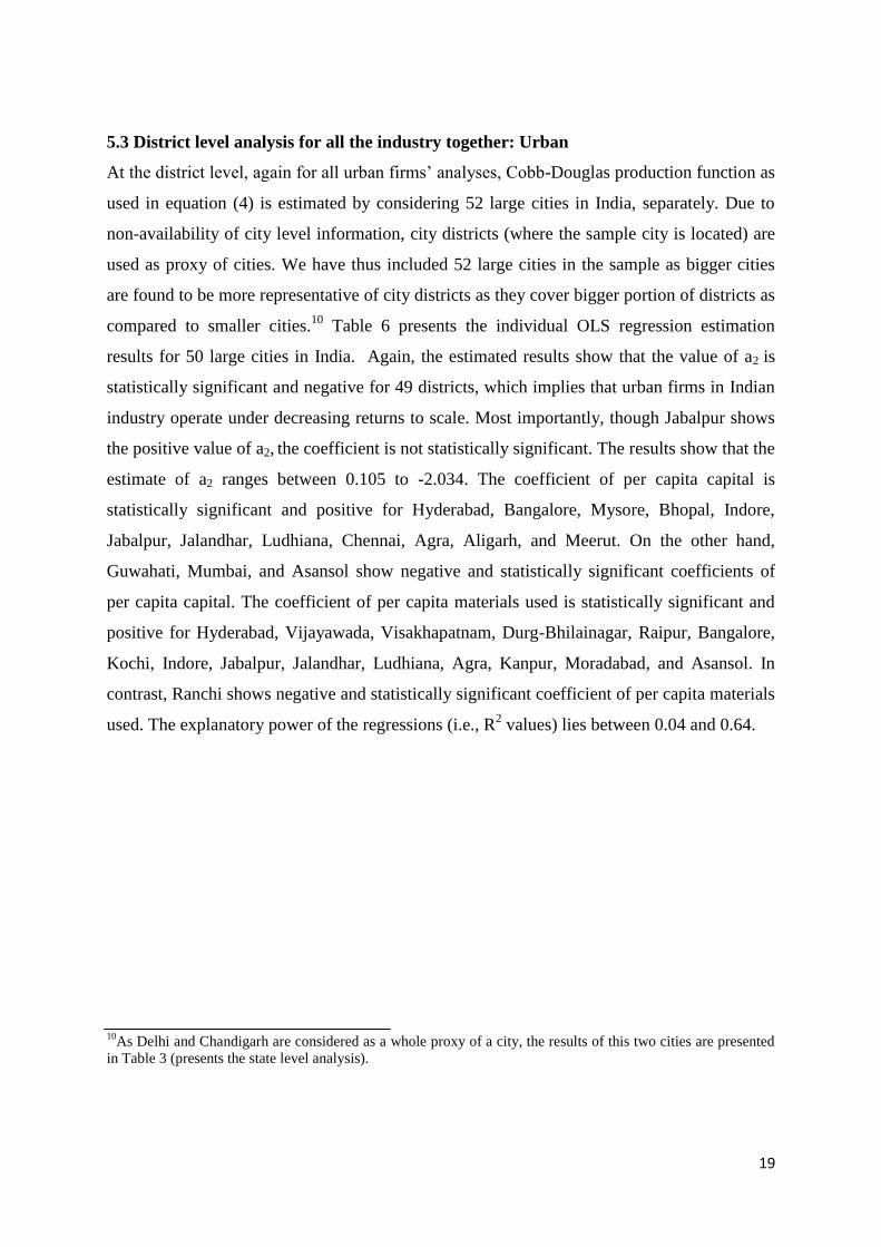
5.3 District level analysis for all the industry together: Urban

At the district level, again for all urban firms‟ analyses, Cobb-Douglas production function as

used in equation (4) is estimated by considering 52 large cities in India, separately. Due to

non-availability of city level information, city districts (where the sample city is located) are

used as proxy of cities. We have thus included 52 large cities in the sample as bigger cities

are found to be more representative of city districts as they cover bigger portion of districts as

compared to smaller cities.10

Table 6 presents the individual OLS regression estimation

results for 50 large cities in India. Again, the estimated results show that the value of a2 is

statistically significant and negative for 49 districts, which implies that urban firms in Indian

industry operate under decreasing returns to scale. Most importantly, though Jabalpur shows

the positive value of a2, the coefficient is not statistically significant. The results show that the

estimate of a2 ranges between 0.105 to -2.034. The coefficient of per capita capital is

statistically significant and positive for Hyderabad, Bangalore, Mysore, Bhopal, Indore,

Jabalpur, Jalandhar, Ludhiana, Chennai, Agra, Aligarh, and Meerut. On the other hand,

Guwahati, Mumbai, and Asansol show negative and statistically significant coefficients of

per capita capital. The coefficient of per capita materials used is statistically significant and

positive for Hyderabad, Vijayawada, Visakhapatnam, Durg-Bhilainagar, Raipur, Bangalore,

Kochi, Indore, Jabalpur, Jalandhar, Ludhiana, Agra, Kanpur, Moradabad, and Asansol. In

contrast, Ranchi shows negative and statistically significant coefficient of per capita materials

used. The explanatory power of the regressions (i.e., R2 values) lies between 0.04 and 0.64.

10As Delhi and Chandigarh are considered as a whole proxy of a city, the results of this two cities are presented

in Table 3 (presents the state level analysis).

20

Table 6: Estimates of Cobb-Douglas Production Function: District Level Urban Firm

Sr. No. Name of the City Constant Independent variables

R2 No. of factory

Capital Labour Materials

1

Hyderabad

10.828***

(1.552)

0.177***

(0.067)

-0.528***

(0.119)

0.210***

(0.070)

0.36

696

2

Vijayawada

9.445***

(2.944)

0.157

(0.096)

-0.446**

(0.190)

0.241***

(0.103)

0.28

429

3

Visakhapatnam

11.077***

(2.373)

0.087

(0.087)

-0.580***

(0.152)

0.288**

(0.131)

0.32

373

4

Guwahati (Gauhati)

17.332***

(2.731)

-0.134*

(0.079)

-0.943***

(0.168)

-0.004

(0.117)

0.46

89

5

Patna

11.169**

(5.015)

0.049

(0.195)

-0.752**

(0.308)

0.269*

(0.155)

0.32

74

6

Durg-Bhilainagar

10.325***

(1.375)

0.096

(0.103)

-0.511***

(0.109)

0.299***

(0.077)

0.39

209

7

Raipur

13.050***

(2.218)

0.084

(0.081)

-0.714***

(0.145)

0.198**

(0.096)

0.38

523

8

Dhanbad

22.344*

(7.663)

-0.218

(0.286)

-1.410**

(0.561)

0.027

(0.194)

0.31

22

9

Jamshedpur

17.288***

(4.849)

-0.266

(0.177)

-0.855***

(0.299)

0.133

(0.211)

0.21

84

10

Ranchi

22.422***

(4.204)

0.051

(0.099)

-1.497***

(0.422)

-0.448**

(0.195)

0.40

30

11

Bangalore

14.678***

(0.676)

0.049*

(0.028)

-0.765***

(0.047)

0.109***

(0.028)

0.33

3943

12

Hubli-Dharwad

14.208***

(2.291)

-0.061

(0.069)

-0.706***

(0.152)

0.179

(0.122)

0.41

242

13

Mysore

13.206***

(3.326)

0.169*

(0.086)

-0.707***

(0.244)

0.070

(0.123)

0.32

295

14

Kochi (Cochin)

8.289***

(2.200)

0.118

(0.099)

-0.313**

(0.140)

0.248**

(0.108)

0.14

482

15

Kozhikode (Calicut)

16.485***

(2.352)

-0.003

(0.058)

-0.906***

(0.174)

0.047

(0.070)

0.58

201

16

Thiruvananthapuram

13.637***

(4.246)

-0.109

(0.263)

-0.629***

(0.200)

0.325

(0.298)

0.37

59

17

Aurangabad

17.471**

(7.035)

0.114

(0.301)

-1.186***

(0.382)

0.162

(0.144)

0.64

21

18

Bhiwandi

14.801***

(2.102)

-0.037

(0.077)

-0.763***

(0.134)

0.062

(0.072)

0.22

326

19

Mumbai (Bombay)

18.667***

(1.273)

-0.101**

(0.041)

-0.988***

(0.091)

-0.010

(0.040)

0.37

752

20

Nagpur

29.642***

(4.574)

-0.193

(0.155)

-2.034***

(0.344)

0.029

(0.135)

0.52

38

21

Nashik

18.235**

(7.907)

0.082

(0.344)

-1.110**

(0.455)

-0.012

(0.181)

0.24

41

22

Pune (Poona)

12.852***

(3.086)

0.138

(0.110)

-0.709***

(0.192)

-0.024

(0.104)

0.34

135

23

Solapur

16.202***

(2.111)

-0.088

(0.135)

-0.946***

(0.140)

0.064

(0.103)

0.64

24

24

Bhopal

11.523***

(2.564)

0.275**

(0.136)

-0.642***

(0.173)

0.159

(0.109)

0.39

180

25

Gwalior

14.436***

(3.973)

-0.057

(0.164)

-0.778***

(0.282)

0.245

(0.234)

0.26

111

26

Indore

12.573***

(1.248)

0.112**

(0.048)

-0.737***

(0.092)

0.244***

(0.057)

0.51

750

21

Table 6 (Continued)

Sr.

No.

Name of the City Constant

Independent variables R

2

No. of

factory Capital Labour Materials

27

Jabalpur

-0.584

(3.996)

0.503***

(0.141)

0.105

(0.289)

0.361*

(0.209)

0.56

86

28

Bhubaneswar

17.249***

(1.916)

0.047

(0.099)

-1.109***

(0.148)

0.085

(0.131)

0.61

46

29

Amritsar

16.087***

(2.119)

-0.012

(0.102)

-0.786***

(0.158)

0.055

(0.072)

0.24

514

30

Jalandhar

13.635

(1.368)

0.205***

(0.056)

-0.764

(0.101)

0.046*

(0.053)

0.33

1383

31

Ludhiana

2.595

(1.779)

0.434***

(0.074)

-0.196

(0.127)

0.317***

(0.052)

0.21

2631

32

Jaipur

17.858***

(2.586)

0.036

(0.075)

-0.887***

(0.162)

0.080

(0.104)

0.48

109

33

Jodhpur

16.611

(15.314)

0.030

(0.223)

-0.776

(1.215)

-0.052

(0.205)

0.04

28

34

Kota

9.142

(8.877)

0.242

(0.345)

-0.433

(0.520)

0.296

(0.249)

0.55

13

35

Chennai (Madras)

15.254***

(1.235)

0.184***

(0.039)

-0.826***

(0.084)

-0.017

(0.049

0.30

2069

36

Coimbatore

18.290***

(0.782)

0.005

(0.030)

-0.994***

(0.056)

0.021

(0.030)

0.33

3829

37

Madurai

20.936***

(3.338)

-0.158

(0.103)

-1.074***

(0.215)

-0.071

(0.111)

0.20

628

38

Salem

16.192***

(2.477)

-0.073

(0.086)

-0.837***

(0.163)

0.139

(0.096)

0.25

650

39

Tiruchirappalli

15.960***

(2.607)

-0.010

(0.102)

-0.790***

(0.170)

0.007

(0.078)

0.20

543

40

Agra

8.155***

(1.474)

0.129*

(0.072)

-0.313**

(0.119)

0.207***

(0.078)

0.21

442

41

Aligarh

6.159**

(2.320)

0.383***

(0.136)

-0.099

(0.139)

-0.035

(0.247)

0.20

159

42

Allahabad

7.487

(4.567)

0.083

(0.141)

-0.220

(0.298)

0.250

(0.200)

0.21

85

43

Bareilly

25.501***

(5.845)

-0.148

(0.156)

-1.438***

(0.429)

-0.152

(0.208)

0.24

144

44

Kanpur

15.724***

(1.592)

-0.022

(0.069)

-0.919***

(0.123)

0.160**

(0.063)

0.36

753

45

Lucknow

15.715***

(3.328)

0.042

(0.103)

-0.872***

(0.242)

-0.006

(0.102)

0.28

337

46

Meerut

7.558***

(2.007)

0.310***

(0.096)

-0.272*

(0.161)

0.022

(0.101)

0.22

367

47

Moradabad

16.415***

(2.066)

-0.081

(0.129)

-0.812***

(0.127)

0.203**

(0.099)

0.34

271

48

Varanasi

(Benares)

6.286

(10.604)

0.443

(0.345)

-0.245

(0.695)

-0.082

(0.685)

0.26

82

49

Asansol

15.159***

(3.837)

-0.005*

(0.160)

-1.114***

(0.263)

0.198***

(0.117)

0.52

41

50

Kolkata

(Calcutta)

19.729**

(8.275)

0.064

(0.174)

-1.277**

(0.574)

-0.231

(0.287)

0.37

50

Notes: 1. Figures in parentheses represent robust standard errors. ***, **, and * indicate

statistical significance at 1%, 5%, and 10% level, respectively.

Source: Estimated by equation (4).

22

5.4 Comparison across all India, state level and district level results: Urban

The estimated results of OLS regression of equation (4) for all India level, state level, and

district level are presented in Table 4, 5, and 6. These results clearly show that the coefficient

(i.e., a2) which represents the degree of returns to scale in urban production is statistically

significant and negative, except for Haryana, Chandigarh, and Jabalpur. Most importantly,

the estimate of a2 ranges between 0.007 to -2.034. The results imply that urban firms in

Indian industry are operating under decreasing returns to scale. The coefficient of per capita

capital is positive and significant for all India level as well as for Andhra Pradesh, Haryana,

Himachal Pradesh, Karnataka, Kerala, Madhya Pradesh, Punjab, Tamil Nadu, Uttar Pradesh,

Uttaranchal, and Chandigarh. In addition, Hyderabad, Bangalore, Mysore, Bhopal, Indore,

Jabalpur, Jalandhar, Ludhiana, Chennai, Agra, Aligarh, and Meerut districts also show the

positive and statistically significant coefficients of per capita capital. The results confirm that

per capita capital has a significant and positive effect on urban production. In contrast,

Jharkhand, Maharashtra, Delhi, Guwahati, Mumbai, and Asansol show negative and

statistically significant coefficient of per capita capital. As the per capita capital is the sum of

private capital and social over head capital, the negative and significant effects of capital on

production indicate that the investment of social over head capital is more heavily allocated

to low income regions or smaller cities. The coefficient of material is statistically significant

and positive for all India level as well as for Andhra Pradesh, Bihar, Chhattisgarh, Haryana,

Himachal Pradesh, Jammu & Kashmir, Karnataka, Kerala, Madhya Pradesh, Punjab, Uttar

Pradesh, Uttaranchal, Chandigarh, and Pondicherry. On the other hand, Hyderabad,

Vijayawada, Visakhapatnam, Durg-Bhilainagar, Raipur, Bangalore, Kochi, Indore, Jabalpur,

Jalandhar, Ludhiana, Agra, Kanpur, Moradabad, and Asansol districts show the positive and

significant effect of per capita materials used on urban production. However, for Ranchi, the

negative and statistically significant coefficient of per capita materials used comes as

surprise.

5.5 All India level analysis for different industry separately: Urban

In section 5.1, 5.2, and 5.3, we have considered all the urban firms together for all India level,

state level, and districts level for the OLS regression estimation without taking different

industrial group separately. But different industries operate with different technology, i.e.,

inter-industry differences may affect the estimates of scale economies. Therefore to allow, for

23

industry fixed (or specific) effects in the model, we estimate Cobb-Douglas production

function for different categories of industries, separately.

The analysis is carried out for 29 industry sectors, grouping firms by their two-digit National

Industry Classification (NIC)-2004 codes: 14 (other mining and quarrying), 15 (manufacture

of food products and beverages), 16 (manufacture of tobacco products), 17 (manufacture of

textiles), 18 (manufacture of wearing apparel), 19 (tanning and dressing of leather), 20

(manufacture of wood and of products of wood and cork), 21 (manufacture of paper and

paper products), 22 (publishing, printing and reproduction of recorded media), 23

(manufacture of coke, refined petroleum products and nuclear fuel), 24 (manufacture of

chemicals and chemical products), 25 (manufacture of rubber and plastic products), 26

(manufacture of other non-metallic mineral products), 27 (manufacture of basic metals), 28

(manufacture of fabricated metal products), 29 (manufacture of machinery and equipment),

30 (manufacture of office, accounting and computing machinery), 31(manufacture of

electrical machinery and apparatus), 32 (manufacture of radio, television and

communication), 33(manufacture of medical, precision and optical instruments, watches and

clocks), 34 (manufacture of motor vehicles, trailers and semi-trailers), 35(manufacture of

other transport equipment), 36(manufacture of furniture; manufacturing), 37 (recycling of

metal waste and scrap), 40(electricity, gas, steam and hot water supply), 50 (sale,

maintenance and repair of motor vehicles and motorcycles), 63 (supporting and auxiliary

transport activities; activities of travel agencies), 92 (recreational, cultural and sporting

activities), and 93 (other service activities).11

11 Although it is possible for grouping into two digit NIC-2004 code for 61 industry sector for all India level,

some of the industry sectors have not been taken into consideration because either these industries sector do not

operate in urban area, or due to small number of observations.

24

Table 7: Estimates of Cobb-Douglas Production Function for Different Industry Sr.

No.

Two digit

Industry code

Constant Independent variables R2 No. of

factory Capital Labour Materials

1 14

17.174***

(1.407)

-0.025

(0.057)

-1.001***

(0.100)

0.122

(0.050)

0.29

1577

2 15

11.642***

(0.520)

0.034*

(0.020)

-0.611***

(0.035)

0.269***

(0.020)

0.30

9927

3 16

11.154***

(1.124)

0.136***

(0.046)

-0.544***

(0.074)

0.166***

(0.048)

0.27

1527

4 17

10.729***

(0.534)

0.063***

(0.021)

-0.533***

(0.036)

0.272***

(0.021)

0.29

6978

5 18

12.237***

(0.784)

0.113***

(0.028)

-0.633***

(0.050)

0.219***

(0.030)

0.34

2925

6 19

12.235***

(1.208)

0.099**

(0.042)

-0.637***

(0.081)

0.169***

(0.050)

0.26

1595

7 20

10.661***

(1.395)

0.031

(0.062)

-0.565***

(0.096)

0.296***

(0.047)

0.30

1086

8 21

11.999***

(1.454)

0.025

(0.057)

-0.594***

(0.097)

0.228***

(0.062)

0.26

1545

9 22

10.167***

(0.986)

0.134***

(0.038)

-0.500***

(0.067)

0.230***

(0.040)

0.32

1918

10 23

9.40***

(1.970)

0.008

(0.090)

-0.271**

(0.135)

0.190**

(0.083)

0.15

183

11 24

9.418***

(0.685)

0.144***

(0.027)

-0.466***

(0.045)

0.255***

(0.027)

0.32

3673

12 25

12.158***

(1.056)

0.126***

(0.041)

-0.629***

(0.072)

0.146***

(0.037)

0.29

2888

13 26

11.969***

(0.921)

0.043

(0.042)

-0.584***

(0.063)

0.206***

(0.038)

0.26

2717

14 27

9.901***

(0.775)

0.060*

(0.033)

-0.493***

(0.053)

0.299***

(0.031)

0.28

2962

15 28

10.376***

(0.802)

0.025

(0.034)

-0.513***

(0.056)

0.336***

(0.029)

0.26

4617

16 29

9.449***

(0.699)

0.123***

(0.029)

-0.482***

(0.048)

0.268***

(0.029)

0.25

4470

17 30

8.689***

(2.185)

0.255***

(0.088)

-0.379**

(0.147)

0.105

(0.109)

0.28

149

18 31

9.504***

(0.878)

0.163***

(0.039)

-0.528***

(0.060)

0.283***

(0.036)

0.34

1869

19 32

8.042***

(1.600)

0.126***

(0.058)

-0.307***

(0.104)

0.285***

(0.060)

0.24

651

20 33

6.798***

(1.624)

0.164***

(0.059)

-0.322***

(0.093)

0.360***

(0.090)

0.25

486

21 34

9.822***

(1.081)

0.131***

(0.036)

-0.533***

(0.073)

0.315***

(0.050)

0.34

1569

22 35

6.942***

(1.276)

0.232***

(0.048)

-0.439***

(0.091)

0.370***

(0.049)

0.33

1357

23 36

12.618***

(1.093)

0.054

(0.042)

-0.601***

(0.074)

0.124***

(0.046)

0.27

1177

24 37

1.640

(4.466)

0.234

(0.155)

-0.056

(0.265)

0.566**

(0.224)

0.44

37

25 40

11.491***

(2.777)

0.042

(0.129)

-0.601***

(0.176)

0.273*

(0.147)

0.29

91

26 50

11.483***

(1.322)

0.122***

(0.046)

-0.578***

(0.091)

0.153***

(0.052)

0.20

2145

27 63

15.939***

(1.935)

-0.043

(0.083)

-0.901***

(0.131)

0.161*

(0.085)

0.42

496

28 92

9.052*

(4.877)

0.121

(0.121)

-0.577

(0.368)

0.539**

(0.229)

0.40

24

29 93

12.970***

(4.290)

0.139

(0.177)

-0.710

(0.313)

0.107

(0.155)

0.37

72

Note: Figures in parentheses represent robust standard errors. ***, **, and * indicate statistical significance

at 1%, 5%, and 10% level, respectively. Source: Estimated by equation (4).

25

For the two digit industry level analysis, again, Cobb-Douglas production function of

equation (4) is used by considering 29 industry groups of all India urban firms. Table 7

presents the regression result for these industrial groups, separately. The results show that the

value of a2 is statistically significant and negative for 26 industrial groups. However, the

coefficient is negative but statistically insignificant for 37 (recycling of metal waste and

scrap), 92 (recreational, cultural and sporting activities), and 93 (other service activities). This

implies that urban firms in Indian industry operate under decreasing returns to scale and the

values of the coefficient a2 range between -0.056 to -1.001. The coefficient of per capita

capital is statistically significant and positive for the industry group 15 (manufacture of food

products and beverages), 16 (manufacture of tobacco products), 17 (manufacture of textiles),

18 (manufacture of wearing apparel), 19(tanning and dressing of leather), 22 (publishing,

printing and reproduction of recorded media), 24 (manufacture of chemicals and chemical

products), 25 (manufacture of rubber and plastic products), 27 (manufacture of basic metals),

29 (manufacture of machinery and equipment), 30 (manufacture of office, accounting and

computing machinery), 31(manufacture of electrical machinery and apparatus), 32

(manufacture of radio, television and communication), 33 (manufacture of medical, precision

and optical instruments, watches and clocks), 34 (manufacture of motor vehicles, trailers and

semi-trailers), 35(manufacture of other transport equipment), and 50 (sale, maintenance and

repair of motor vehicles and motorcycles). The coefficient of per capita materials used also

show positive and statistically significant effect on urban production, except for industry

groups14 (other mining and quarrying) and 93 (other service activities). The estimated results

indicate that per capita capital and materials used have a positive and statistically significant

effect on urban production.

5.6 Analysis for different industry located in 52 large city districts: Urban

In section 5.5, we estimate the Cobb-Douglas production function for different categories of

industries located in all India urban areas, separately. However, as Krugman (1991) core-

periphery model explains, the realization of economies of scale through minimizing

transportation cost occurs in the region with larger demand, i.e., “Core region”. Therefore, we

consider 52 large cities in India as a proxy of “core regions” and measure the agglomeration

economies for different industries located in these 52 larger cities in India.

26

Table 8: Estimates of Cobb-Douglas Production Function for different industries located in

52 Large Cities

Sr.

No. Two digit industry

code

Independent variables

Constant R2

No. of

factory Capital Labour Materials

1 14

-0.070

(0.189)

-1.273**

(0.491)

-0.470**

(0.208)

24.155***

(6.303)

0.26

160

2 15

-0.015

(0.037)

-0.560***

(0.064)

0.147***

(0.037)

12.620***

(0.912)

0.18

2436

3 16

0.123

(0.103)

-0.732***

(0.210)

0.123

(0.104)

13.513***

(2.853)

0.37

187

4 17

0.012

(0.034)

-0.694***

(0.056)

0.162***

(0.033)

13.614***

(0.826)

0.23

4154

5 18

0.113***

(0.037)

-0.688***

(0.065)

0.139***

(0.038)

13.450***

(1.035)

0.32

1765

6 19

0.029

(0.055)

-0.724***

(0.109)

0.132*

(0.068)

14.181***

(1.613)

0.29

731

7 20

0.136

(0.102)

-0.323*

(0.173)

0.214**

(0.086)

8.503***

(2.281)

0.18

278

8 21

-0.044

(0.112)

-0.691***

(0.161)

0.123

(0.089)

13.955***

(2.499)

0.21

565

9 22

0.204***

(0.050)

-0.526***

(0.094)

0.140**

(0.061)

10.664***

(1.405)

0.31

974

10 23

-0.061

(0.143)

-0.152

(0.213)

0.440***

(0.114)

7.380**

(2.943)

0.27

56

11 24

0.123***

(0.046)

-0.520***

(0.083)

0.199***

(0.047)

10.613***

(1.245)

0.30

1283

12 25

0.248***

(0.065)

-0.535***

(0.118)

0.047

(0.058)

11.091***

(1.742)

0.26

1043

13 26

0.267***

(0.090)

-0.449***

(0.143)

0.122

(0.086)

9.632***

(2.040)

0.30

581

14 27

0.043

(0.049)

-0.472***

(0.082)

0.320***

(0.051)

9.772***

(1.194)

0.24

1322

15 28

0.049

(0.047)

-0.637***

(0.070)

0.254***

(0.043)

12.141***

(1.048)

0.26

2580

16 29

0.112**

(0.044)

-0.693***

(0.075)

0.131***

(0.047)

12.574***

(1.097)

0.23

2277

17 30

0.053

(0.126)

-0.822***

(0.238)

-0.088

(0.180)

16.150***

(3.620)

0.45

74

18 31

0.185***

(0.053)

-0.611***

(0.090)

0.128**

(0.052)

11.289***

(1.318)

0.35

987

19 32

-0.011

(0.077)

-0.559***

(0.166)

0.126

(0.086)

12.862***

(2.362)

0.20

347

20 33

0.020

(0.081)

-0.645***

(0.135)

0.024

(0.099)

14.277***

(2.161)

0.22

225

21 34

0.127**

(0.060)

-0.579***

(0.115)

0.165**

(0.070)

11.221***

(1.651)

0.30

644

22 35

0.295***

(0.065)

-0.437***

(0.135)

0.390***

(0.070)

6.106***

(1.931)

0.32

973

23 36

0.002

(0.044)

-0.672***

(0.087)

0.054

(0.054)

14.360***

(1.211)

0.30

708

24 37

0.021

(0.742)

-0.157

(0.758)

0.788

(0.918)

2.722

(12.437)

0.41

7

25 40

-0.113

(0.191)

-0.894***

(0.314)

0.220

(0.281)

16.579***

(5.307)

0.29

40

26 50

0.180***

(0.063)

-0.460***

(0.138)

0.204**

(0.083)

9.436***

(1.952)

0.19

1169

27 63

-0.185

(0.235)

-0.725**

(0.319)

0.277

(0.250)

14.590***

(4.698)

0.28

132

28 93

-0.024*

(0.184)

-0.675

(0.378)

0.167

(0.144)

13.731**

(5.327)

0.37

59

Note: Figures in parentheses represent robust standard errors. ***, **, and * indicate statistical significance at

1%, 5%, and 10% level, respectively.

Source: Estimated by equation (4).

27

Table 8 presents the regression result of equation (4) for 28 industrial (two digit level)

groups, separately. The results show that the value of a2 is negative for 28 industrial groups

and statistically significant for 26 industrial groups, except for industrial groups 23

(manufacture of coke, refined petroleum products and nuclear fuel) and 93 (other service

activities). The results imply that urban firms in Indian industries those are located in 52

largest cities operating under decreasing returns to scale and the values of a2 ranges between -

0.152 to -1.273. The regression results also find that the coefficient of per capita capital is

positive and statistically significant for industry groups18 (manufacture of wearing apparel),

22 (publishing, printing and reproduction of recorded media), 24 (manufacture of chemicals

and chemical products), 25 (manufacture of rubber and plastic products), 26 (manufacture of

other non-metallic mineral products), 29 (manufacture of machinery and equipment),

31(manufacture of electrical machinery and apparatus), 34 (manufacture of motor vehicles,

trailers and semi-trailers), 35(manufacture of other transport equipment), and 50 (sale,

maintenance and repair of motor vehicles and motorcycles). The coefficients of per capita

materials used are statistically significant and positive for industry groups15 (manufacture of

food products and beverages), 17 (manufacture of textiles), 18 (manufacture of wearing

apparel), 19 (tanning and dressing of leather), 20 (manufacture of wood and of products of

wood and cork), 22 (publishing, printing and reproduction of recorded media), 23

(manufacture of coke, refined petroleum products and nuclear fuel), 24 (manufacture of

chemicals and chemical products), 27 (manufacture of basic metals), 28 (manufacture of

fabricated metal products), 29 (manufacture of machinery and equipment), 31(manufacture of

electrical machinery and apparatus), 34 (manufacture of motor vehicles, trailers and semi-

trailers), 35(manufacture of other transport equipment), 36(manufacture of furniture;

manufacturing), and 50 (sale, maintenance and repair of motor vehicles and motorcycles).

The results indicate that per capita capital and materials used have a positive and significant

effect on urban production. However, the coefficient of per capita capital for industry group

93 (other service activities) and the coefficient of per capita materials used for industry

group14 (other mining and quarrying) are negative and statistically significant.

5.7 Largest industry of a large city districts: Urban

Finally, in order to measure the scale economies especially for a largest (in terms of number

of firms) industry operating in a specific large city (or “core region”), we measure the

agglomeration economies for different industries located in different large cities in India.

28

Here, we consider the industry of a city which has the highest number of firms located in that

particular city, and we call this industry as the largest industry of this city. Table 9 presents

the regression result of equation (4) for 27 districts.12

The results show that among 27 large

city districts, the largest industries of 18 districts operate under decreasing returns to scale, as

the value of coefficient a2 is negative and statistically significant. However, the value of a2 is

positive for industry groups15 (manufacture of food products and beverages) located in

Vijayawada, 27 (manufacture of basic metals) located in Patna, 29 (manufacture of

machinery and equipment) located in Mysore and Chandigarh. But the coefficient a2 is not

statistically significant. The values of a2 range between 0.764 and -1.506. The coefficient per

capita capital is positive and significant only for industry group 29 (manufacture of

machinery and equipment) located in Jalandhar out of 27 city districts. The coefficients of per

capita materials used are positive and statistically significant for industry groups 15

(manufacture of food products and beverages) located in Vijayawada and Indore, 27

(manufacture of basic metals) located in Visakhapatnam and Durg-Bhilainagar, 18

(manufacture of wearing apparel) located in Chennai, 17 (manufacture of textiles) located in

Salem, 19 (tanning and dressing of leather) located in Agra and Kanpur, 29 (manufacture of

machinery and equipment) located in Chandigarh.

12 Though we have considered 52 large city districts for the analysis, we report here 27 districts due to small

number of observation of a largest industry group of a particular district.

29

Table 9: Estimates of Cobb-Douglas Production Function for different largest industry located in different

Large Cities Sr.

No. Cities

Two Digit

Industry code Constant

Independent variable

R2

No. of

factory Capital Labour Materials

1

Hyderabad

15

14.206***

(4.755)

0.120

(0.141)

-0.742**

(0.323)

0.205

(0.205)

0.61

116

2

Vijayawada

15

-0.615

(7.245)

0.381

(0.228)

0.205

(0.508)

0.420**

(0.199)

0.36

104

3

Visakhapatnam

27

5.839*

(3.069)

0.065

(0.146)

-0.283

(0.233)

0.525**

(0.195)

0.49

88

4

Patna

27

-7.364

(13.470)

0.544

(0.502)

0.764

(0.747)

0.179

(0.411)

0.15

12

5

Durg-Bhilainagar

27

11.316***

(2.148)

0.106

(0.121)

-0.568***

(0.168)

0.291**

(0.104)

0.60

97

6

Raipur

27

13.200***

(3.391)

-0.028

(0.150)

-0.655***

(0.219)

0.252

(0.192)

0.42

146

7

Bangalore

18

17.851***

(1.794)

-0.048

(0.064)

-0.935***

(0.108)

0.100

(0.063)

0.39

607

8

Mysore

29

2.609

(7.414)

0.270

(0.225)

0.268

(0.606)

0.095

(0.244)

0.16

59

9

Kochi (Cochin)

24

11.933*

(5.959)

0.227

(0.236)

-0.748*

(0.363)

0.272

(0.209)

0.48

63

10

Bhiwandi

24

9.059*

(4.537)

0.138

(0.170)

-0.490

(0.295)

0.205

(0.145)

0.30

73

11

Mumbai

(Bombay)

37

19.188***

(1.967)

-0.065

(0.055)

-1.008***

(0.173)

-0.112**

(0.059)

0.35

221

12

Pune (Poona)

29

8.530

(7.570)

0.150

(0.238)

-0.521

(0.498)

0.275

(0.209)

0.36

39

13

Indore

15

13.751***

(4.898)

-0.197

(0.148)

-0.699*

(0.338)

0.268*

(0.151)

0.34

237

14

Amritsar

17

14.185***

(3.354)

0.063

(0.179)

-0.700***

(0.226)

0.092

(0.095)

0.28

212

15

Jalandhar

29

18.552***

(2.302)

0.168*

(0.093)

-1.154***

(0.176)

-0.054

(0.078)

0.43

578

16

Ludhiana

17

8.801**

(3.520)

0.233

(0.142)

-0.488*

(0.261)

0.066

(0.092)

0.12

765

17

Chennai (Madras)

18

16.183***

(2.088)

0.172

(0.064)

-0.920***

(0.135)

0.002***

(0.079)

0.41

540

18

Coimbatore

17

17.811***

(0.994)

-0.014

(0.038)

-0.953***

(0.069)

0.058

(0.043)

0.34

2182

19

Madurai

15

22.570***

(8.194)

-0.183

(0.213)

-1.115*

(0.557)

-0.170

(0.206)

0.12

212

20

Salem

17

15.180***

(3.260)

-0.035

(0.114)

-0.774***

(0.210)

0.147**

(0.080)

0.37

197

21

Tiruchirappalli

28

15.736***

(5.602)

-0.094

(0.254)

-0.780**

(0.308)

0.145

(0.151)

0.32

178

22

Agra

19

5.562***

(2.808)

0.149

(0.098)

-0.201

(0.174)

0.372**

(0.162)

0.35

83

23

Kanpur

19

23.654***

(3.132)

-0.138

(0.178)

-1.506

(0.230)

0.040***

(0.163)

0.45

154

24

Meerut

17

11.372***

(2.749)

0.303

(0.216)

-0.605***

(0.193)

0.032

(0.201)

0.41

114

25

Moradabad

29

15.482***

(2.522)

0.022

(0.150)

-0.756***

(0.151)

0.161

(0.121)

0.34

191

26

Chnadigarh

29

0.716

(4.896)

0.346

(0.222)

0.014

(0.393)

0.492**

(0.107)

0.44

103

27

Delhi

18

19.152***

3.712)

-0.096

(0.127)

-0.876***

(0.207)

0.048

0.138)

0.29

186

Note: Figures in parentheses represent robust standard errors. ***, **, and * indicate

statistical significance at 1%, 5%, and 10% level, respectively.

Source: Estimated by equation (4).

30

5.8 Comparison between all India, state level and district level results for different

Industry groups: Urban

In sections 5.5, 5.6, and 5.7, we measure the agglomeration economics for firms in different

industries those located in all India level urban areas or located in 52 larger cities in India.

The results are presented in Table 7, 8, and 9; the results show that the value of a2 is negative

and statistically significant for all the firms in different industries. However, the value of a2 is

positive but statistically insignificant for industry groups 15 (manufacture of food products

and beverages) located in Vijayawada, 27 (manufacture of basic metals) located in Patna, 29

(manufacture of machinery and equipment) located in Mysore and Chandigarh. The results

confirm that Indian urban firms under different industries are operating under decreasing

returns to scale and the estimated values of a2 range between -0.056 to 0.764. The results also

indicate that in many cases the coefficient of per capita capital and materials used have

positive and statistically significant effects on urban production. In contrast, the coefficient

of per capita capital is negative and significant for industry group 93 (other service activities).

Moreover, the coefficient of per capita materials used is statistically significant and negative

for industry groups 14 (other mining and quarrying) located in 52 large city districts and 37

(recycling of metal waste and scrap) located in Mumbai district. The result of negative and

significant per capita capital and materials used comes as surprise.

Our findings, i.e., the decreasing returns to scale at firm level support the findings of Lall et

al. (2004), Lall and Rodrigo (2001), and Ghani et al. (2012) for Indian firms. However, this

result does not support the findings of Kanemoto et al., (1996) in regard to Japan and Rinaldi

and Nurwita (2011) in regard to Indonesia. However, the result of negative effect of social

overhead capital on urban production for some industries (or firms) supports the findings of

Kanemoto et al., (1996).

6 Conclusions and Policy Implications

The estimated results show that urban firms in Indian industry operate under decreasing

returns to scale in urban production irrespective of at all India urban level and large city level.

Economies of scale for all the urban firms together, ranges between -0.492 and -0.612 for all

India level, 0.007 and -1.305 for 26 state level, and 0.0105 and -2.034 for 52 large city level.

On the other hand, different industries specific analyses show that economies of scale lies

between -0.056 and -1.001 for all India level, -0.152 and -1.273 for 52 large city levels and

0.764 to -1.506 for different city specific largest industries level.

31

The firms located in Haryana, Chandigarh, and Jabalpur show positive and statistically

insignificant economies of scale. In addition, industry groups 15 (manufacture of food

products and beverages) located in Vijayawada, 27 (manufacture of basic metals) located in

Patna, 29 (manufacture of machinery and equipment) located in Mysore and Chandigarh also

show statistically insignificant but positive economies of scale. The results indicate that

Indian urban firms under different industries are operating under decreasing returns to scale.

The results show that for a large numbers of firms (or industries) per capita capital and

materials used have a positive and statistically significant effect on urban production.

From this analysis it appears to be counterintuitive about the influence of increasing returns

to scale for regional concentration of firms (or industries) in Indian urban sector. Our findings

may also support the “folk theorem” of location theory, which says that in the absence of

increasing returns, there will be “backyard capitalism,” with production potentially locating

wherever there is demand. Finally, we conclude that Indian manufacturing urbanization

seems to be less important for urban economic growth.

Therefore, we suggest that firm level or industry specific and location specific (aimed at

unites operating at different levels such as small towns/metros/large urban agglomerations)

policies are required for the promotion of concentration of urban firms to absorb the

advantage of increasing returns to scale for higher production.

However, in consideration of different econometric specification and different variables

pertaining to different periods of time applied to estimate the economies of scale for urban

firms, the estimated results are open to further scrutiny.

32

References:

Aso, Y. (2008) Social overhead capital development and geographical concentration. Policy

Research Institute, Ministry of Finance, Japan, Public Policy Review, 4: 111-132.

Besley, T. and Burgess, R. (2004) Can labour regulation hinder economic performance?

Evidence from India. Quarterly Journal of Economics, 119: 91-134.

Chakravorty, S. (2003) Industrial location in post‐reform India: patterns of interregional

divergence and intraregional convergence. Journal of Development Studies, 40:120‐52.

Chakravorty, S., Koo, J., Lall, S.V (2005) Do localization economies matter in cluster

formation? Questioning the conventional wisdom with data from Indian metropolises.

Environment and Planning A, 37: 331-353.

CSO (2008) National accounts statistics 2008. Central statistical organisation, ministry of

statistics and programme implementation, Government of India.

CSO (2010) National accounts statistics 2010. Central statistical organisation, ministry of

statistics and programme implementation, Government of India.

Doms, M.E. (1992) Essays on capital equipment and energy technology in the manufacturing

sector. PhD Dissertation. University of Wisconsin at Madison.

Fernandes, A. and Sharma, G. (2012) Together we Stand? Agglomeration in Indian

manufacturing. Policy Research Working Paper No. 6062, World Bank.

Fujita, M., Mori, T., Henderson, J.V., Kanemoto, Y. (2004) Spatial distribution of economic

activities in Japan and China. In V. Henderson and J.F. Thisse (eds) Handbook of

Regional and Urban Economics, Vol. 4. Amsterdam: North-Holland.

Fujita, M. (2007) The development of regional integration in East Asia: from the viewpoint

of spatial economics. Review of Urban and Regional Development Studies, 19: 2–20.

Ghani, E., Goswami, A.G., Kerr, W.R. (2012) Is India‟s manufacturing sector moving away

from cities? Working Paper No. 17992, National Bureau of Economic Research,

Cambridge, Massachusetts.

Greenhut, J. and Greenhut, M.L. (1975) Spatial price discrimination, competition and

locational effects. Economica, 42: 401- 419.

Government of India [GOI] (2009) Report of the High Level Committee on Estimation of

Saving and Investment. Ministry of Statistics and Programme Implementation, New Delhi

Henderson, J. V., Shalizi, Z., Venables, A.J. (2000) Geography and development. Journal

of Economic Geography, 1: 81-105.

Hotelling, H. (1929) Stability in competition. Economic Journal, 39: 41-57

Isard, W. (1956) Location and Space-economy. MIT Press, Cambridge, MA.

Kanemoto, Y. (1990) Optimal cities with indivisibility in production and interactions

between firms. Journal of Urban Economics, 27: 46–59.

Kanemoto, Y., Ohkawara, T., Suzuki, T. (1996). Agglomeration economies and a test for

optimal city sizes in Japan. Journal of the Japanese and International Economies,10: 379-

398.

Kanemoto, Y., Kitagawa, T., Saito, H., Shioji, E. (2005) Estimating urban agglomeration

economies for Japanese metropolitan areas: Is Tokyo Too large? In A. Okabe (eds) GIS-

Based studies in the Humanities and Social Science. Taylor &Francis, Boca Raton,

Krugman, P. (1991) Increasing returns and economic geography. Journal of Political

Economy, 99: 483-499.

Krugman, P. (1999) The role of geography in development. International Regional Science

Review, 22: 142-161.

Lall, S. and Rodrigo, C. (2001) Perspective on the sources of heterogeneity in Indian

Industry. World Development, 29: 2127-2143.

33

Lall, S. V., Koo, J., Chakravorty, S. (2003) Diversity matters: the economic geography of

industry location in India. Policy Research Working Paper 3072, The World Bank.

Lall, S., Shalizi, Z., Deichmann, U. (2004) Agglomeration economies and productivity in

Indian industry. Journal of Development Economics,73: 643-673.

Lall, S. V. and Mengistae, T. ( 2005a) Business environment, clustering, and industry

location : evidence from Indian cities. Policy Research Working Paper Series 3675, The

World Bank.

Lall, S.V. and Mengistae, T. (2005b) The Impact of business environment and economic

geography on plant-level productivity: an analysis of Indian industry. Working Paper No.

S3664, World Bank.

Lall, S. and Chakravorty, S. ( 2005) Industrial location and spatial inequality: theory and

evidence from India. Review of Development Economics, 9: 47-68.

Lösch, A. (1940) Die Räumliche Ordnung der Wirtschaft (Gustav Fischer, Jena). English

translation The Economics of Location, Yale University Press, New Haven CN, 1954.

Mani, M., Pargal, S., Huq, M. (1996) Does Environmental Regulation Matter? Determinants

of the Location of New Manufacturing Plants in India in 1994. World Bank Working

Paper 1718, World Bank: Washington DC.

Marshall, A. (1890) Principles of Economics. London: Macmillan.

Mukherjee, V. (2008) Trade policy and increasing return based agglomeration: is there any

evidence in India? Working Paper No. 07-08, Department of Economics , Jadavpur

University.

Ottaviano, G. I. P. and Thisse. J.-F. (2004) Agglomeration and Economic Geography. In V.

Henderson and J.F. Thisse (eds) Handbook of Regional and Urban Economics, Vol. 4.

Amsterdam: North-Holland.

Ottaviano, G.I.P. and Thisse, J.-F. (2005) New economic geography: what about the N.

Environmental and Planning A, 37: 1707-25.

Puga, D. (2010) The magnitude and causes of agglomeration. Journal of Regional Science,

50: 203-219.

Rajaraman, I., Mukhopadhyay, H., Bhatia, N. (1999) Fiscal Industrial Incentives of the

Government of Madhya Pradesh: Costs and Benefits. Mimeo, NIPFP: New Delhi.

Reeding, S. (2010) The empiric of new economic geography. Journal of Regional Science,

50: 297-311.

Rinaldi, R. and Nurwita, E. (2011) Rise and fall of cities, measuring spatial clustering and

economies of urban agglomeration in West Java. Working Papers in Economics and

Development Studies (WoPEDS) 201104, Department of Economics, Padjadjaran

University.

Sridhar, K. S. and Wan, G. (2010) Firm location choice in cities: evidence from China, India,

and Brazil. China Economic Review, 21: 113-122.

Sridhar K.S. (2005) Incentives for Regional Development: Competition among Sub-National

Governments, Palgrave Macmillan: Basingstoke.

Starrett, D. (1978) Market allocations of location choice in a model with free mobility.

Journal of Economic Theory, 17: 21-37.

Tulasidhar, V. B. and Rao, M.G. (1986) Cost and efficacy of fiscal incentives: the case of

sales tax subsidy. Economic and Political Weekly, 21:1799-806.

Weber, A. (1909) Ueber den Standort der Industrien, Tübingen J. C. B. Mohr. English

translation: The Theory of the Location of Industries, Chicago, Chicago University Press,

1929.

World Bank (2004) India: Investment climate and manufacturing industry. Washington:

World Bank.