MPRAMunich Personal RePEc Archive

Loss Aversion, Expectations andAnchoring in the BDM Mechanism

Achilleas Vassilopoulos and Andreas C. Drichoutis and

Rodolfo Nayga

Agricultural University of Athens, University of Arkansas

22 March 2018

Online at https://mpra.ub.uni-muenchen.de/85635/MPRA Paper No. 85635, posted 1 April 2018 21:40 UTC

Loss Aversion, Expectations and Anchoring in the BDMMechanism∗

Achilleas Vassilopoulos†1,2, Andreas C. Drichoutis‡2, and Rodolfo M. Nayga,Jr.§3

1ICRE8: International Centre for Research on the Environment and theEconomy

2Agricultural University of Athens3University of Arkansas

Abstract: We present the results of an economic laboratory experiment that tests be-

havioral biases that have been associated with the BDM mechanism. By manipulating the

highest random competing bid, the maximum possible loss, the distribution of prices and

the elicitation format, we attempt to disentangle the effects of reference-dependence, expec-

tations as well as price and loss anchoring on subjects’ bids. The results show that bids are

affected by expectations and anchoring on the highest price but not by anchoring on the max-

imum possible loss. In addition, results are supportive of the no-loss-in-buying hypothesis

of Novemsky and Kahneman (2005).

Keywords: Becker-DeGroot-Marschak (BDM) mechanism; expectations; anchoring;

valuation; experiment.

JEL Classification Numbers: C91, D44.

∗We would like to thank Angelos Lagoudakis and Manos Petrakis for helpful research assistance. Approvalfor the research was provided by the Board of Ethics and Deontology of the Department of AgriculturalEconomics & Rural Development at the Agricultural University of Athens (2/2015).†Corresponding author: Senior Researcher, International Centre for Research on the Environment and the

Economy, Artemidos 6 & Epidavrou, 15125, Maroussi, Athens, Greece and Department of Agricultural Eco-nomics & Rural Development, Agricultural University of Athens, tel:+30-210-6875346, e-mail: avas@aua.gr,achilleas.vassilopoulos@icre8.eu.‡Assistant professor, Department of Agricultural Economics & Rural Development, Agricultural Univer-

sity of Athens, Iera Odos 75, 11855, Greece, tel: +30-210-5294781, e-mail: adrihout@aua.gr.§Distinguished Professor and Tyson Endowed Chair, Department of Agricultural Economics & Agribusi-

ness, University of Arkansas, Fayetteville, AR 72701, USA, and NBER, tel:+1-4795752299 e-mail:rnayga@uark.edu.

1

1 Introduction

The Becker-DeGroot-Marschak (BDM) mechanism (Becker et al., 1964) is a well known

incentive-compatible mechanism, frequently used in experimental economics and in non-

market valuation. It is a very important tool for measuring subjects’ valuations both inside

and outside the lab and thus widely used in the marketing field for the valuation of novel

products and product attributes. In experimental economics, the BDM mechanism is usually

employed for the valuation of lotteries or tokens, to examine agents’ risk/time preferences

or departures from standard economic models of individual behavior. As a testament to

its popularity, Becker et al. (1964) count more than 2,100 citations in Google Scholar as of

March 2018. From a theoretical point of view, the mechanism is strategically equivalent to

a Vickrey auction against an unknown bidder (Vickrey, 1961) and thus it is often referred

to as an additional auction format.

The BDM mechanism is simple and presumed to induce truth-telling since based on

Expected Utility Theory (EUT), it is in the best interest of bidders to report their true

value for the object, irrespective of other factors such as their risk preferences. In addition,

if preferences do not violate the von Neumann-Morgenstern axioms and in particular the

dominance axiom, BDM bids should equal one’s true value for the goods, independent of

the underlying price distribution from which the binding price is randomly drawn. This

is also true even with loss-averse agents in the case that decision weights are linearized to

be probabilities.1 However, Karni and Safra (1987) showed that the BDM is not incentive-

compatible in valuing lotteries, even for rational agents (i.e., those that do not violate the

weak-ordering axiom). They attributed the phenomenon of preference reversals that is of-

ten observed in implied choices between lotteries using the BDM, to the violation of the

independence axiom. Horowitz (2006) also pointed out that the BDM may not be incentive-

compatible even when the objects involve no uncertainty, as in the case of regular products.

Other studies (discussed in Section 2) have also questioned the usefulness of the mechanism

in the presence of behavioral biases, such as expectations-based loss aversion and anchoring.

Some researchers doubt that the BDM is appropriate to study these biases, as participants’

bids are not even error-prone signals of true preferences (Cason and Plott, 2014). Addi-

tional issues have also been raised related to the effect of wording used in the experimental

instructions and subjects’ anonymity (Plott and Zeiler, 2004, 2007).

We revisit these behavioral issues associated with the BDM mechanism discussed above.

Unlike previous attempts to manipulate expectations through exogenous lotteries (Marzilli Er-

1Note that by true value, we mean the highest deterministic price at which the subject would decide tobuy the object in a relevant market. Thus, we make the plausible assumption that a subject who is lossaverse in the experiment will also be loss averse in the respective market.

2

icson and Fuster, 2011; Smith, 2012), we use procedures that mimic those of the typical

mechanism. Our procedures avoid signaling the “objective” value of the auctioned good or

causing misconceptions, especially given the added complexity that exogenous lotteries could

introduce to the mechanism.2 In addition, we control for price and loss anchoring effects

that may be present in previous studies (e.g., Banerji and Gupta, 2014; Bohm et al., 1997)

and are related to the highest price and the maximum possible loss.3

In the BDM format that we employ in this study, the virtual urn used for determining

the random binding price has numbered outcomes instead of prices outcomes, with each

number mapping onto a price from a predetermined range. This mapping is used as an

experimental design variable where for example, the numbers {1, 2, . . . , 120} correspond to

prices {e0.1, e0.2, . . . , e12.0} in one treatment and to the prices {e0.1, e0.2, . . . , e6.0}in another. We posit that the use of numbers facilitates decoupling of expectations about

getting the auctioned good — which in our design are given by the relative frequencies of

the numbered outcomes — with price anchors that are affected by the highest and lowest

possible price outcomes. By doing so, we implicitly assume that anchoring of bids on the

numbered outcomes is not likely to happen. This is mainly for two reasons: 1) numbers

are not expressed on the money scale and are therefore irrelevant as bidding anchors 2) the

numbers are implausibly large in relation to a subject’s potential bid (in our experiment

numbers in the virtual urn run from 1 to 60 or from 1 to 120). Previous research supports

these assumptions, showing that anchors of an item’s value in years of life expectancy did

not affect judgments of its dollar value and vice-versa (Chapman and Johnson, 1994) or that

passive or active number searches or implausible anchors do not affect bids in incentivized

willingness-to-pay (WTP) elicitation experiments (Sugden et al., 2013).

Finally, another modification of the mechanism we use in our design is that we do not have

a one-to-one correspondence between actual payments (losses) and prices in all treatments,

unlike the usual BDM where the maximum amount a subject may pay is her bid. Thus, as

explained momentarily, we separate price anchors from loss anchors (which are driven by the

highest and lowest possible loss, respectively) that are expected to have opposite effects.

In the next section, we review the biases relevant to the BDM mechanism that we are

examining in the current study. We then present our experimental design in Section 3, then

2For example, the high or low probability of winning the prize to be auctioned later, may be perceivedas a signal of good value e.g., a higher probability might indicate a less valuable prize. In addition, in caseswhere both the draw regarding whether subjects will be able to trade and the random price determinationare done simultaneously, the participants might face difficulties to assign the correct probability in eachstate.

3As explained below, the highest price could anchor subjects’ bids causing price anchoring while themaximum possible loss could make the utility dimensions related to money more salient and thus cause lossanchoring.

3

the results and conclude in the last section.

2 Behavioral biases and the BDM mechanism

In this section, we discuss the behavioral biases that have been related to the BDM

mechanism. We also cite the relevant literature that has tried to explore these biases and

discuss how our experiment differs from these past studies.

2.1 Expectations

The idea of expectations-based loss aversion was introduced in Koszegi and Rabin (2006)

who presented a model that is similar to prospect theory (Kahneman and Tversky, 1979;

Tversky and Kahneman, 1991) but where the reference points are formed by expectations

(instead of the status-quo). Smith (2008, 2012) was the first to test this model in the context

of the BDM mechanism. In his experiments, just before the valuation task, subjects took

part in a lottery with a university mug as the prize. The high (low) probability group was

informed that they would be given the opportunity to get the mug with a probability of

70% (10%). The subjects who were given the opportunity to purchase the mug were allowed

to participate in a BDM procedure by stating their maximum WTP for the mug. Results

showed that although assignment to the high probability of winning the prize produced a

small increase in valuation, this effect was not statistically significant.

Marzilli Ericson and Fuster (2011) elicited willingness-to-accept (WTA) values for a uni-

versity mug using a similar design to Smith (2008, 2012). In their high (low) probability

treatment, there was a 80% (10%) chance that subjects would get a mug for free (and then

participate in a BDM experiment to sell it) and a 10% (80%) chance that they would get

nothing (and thus not take part in the subsequent BDM procedure). Besides the elicitation

format (WTP vs. WTA), the main difference with the experiments of Smith (2008, 2012)

was that subjects submitted their bid before they knew the realized state of nature, namely

before they reached the point where they knew whether their bids would actually matter

(i.e whether they will have the chance to participate in the BDM). Marzilli Ericson and

Fuster (2011) found a 20%-30% higher valuation in the high probability treatment which

they attributed to the induced higher expectation of being able to leave the experiment with

the mug as compared to the low expectation treatment.

In addition to the studies cited above, Banerji and Gupta (2014) provided theoretical

and experimental results that confirm the role of expectations in the BDM mechanism.

They varied the support of the randomly drawn bid for a chocolate and found a significant

4

difference in valuations, a result which is in accordance with expectation-based reference

points. Bohm et al. (1997) on the other hand, manipulated the uniform price support in a

BDM experiment and found a reverse effect of expectations on WTA bids for petrol coupons.

Other relevant studies include Mazar et al. (2013) who tested the sensitivity of valuations to

the underlying distribution in the BDM using travel mugs and Amazon vouchers; Urbancic

(2011) using a within-subjects design and a gift certificate product redeemable for cookies;

and Tymula et al. (2016) who used products with higher market values such as a backpack,

an iPod Shuffle, and a pair of noise-canceling headphones. Although all these studies did

not explicitly refer to expectation-based preferences (with the exception of Tymula et al.,

2016) but rather examined the distributional dependence of the valuations, a closer look at

their results suggest patterns that are opposite to the ones expected under the Koszegi and

Rabin (2006) model of behavior.

2.2 Price anchoring

Besides expectations, anchoring is a well-known behavioral anomaly first detected by

Tversky and Kahneman (1974) in their famous wheel-of-fortune experiment. Tversky and

Kahneman (1974) used a wheel of fortune with numbers between 0 and 100 that was actually

rigged to stop only on 10 or 65. They found a significant effect of the drawn number

on subjects’ estimates of the number of African countries in the UN and concluded that

respondents do not have predefined values and are thus using any given anchor to make a

series of dynamic adjustments towards their final estimate. Because these adjustments are

insufficient, the subjects end up with estimates that are close to the anchor. In a typical

BDM experiment, although subjects are not explicitly asked to compare their WTP with any

other value, it is possible that they start the formulation of their bids by comparing their

value to relevant anchors. Another more convincing explanation in terms of non-market

valuation is that anchoring biases might be based on the concept of associative coherence

(Morewedge and Kahneman, 2010). According to this concept, anchors (even unrealistic

ones) bring to mind coherent attributes that would justify such an anchor. For example, a

high price anchor in an auction would urge subjects into thinking of the quality attributes

that would justify such a high price, while in the case of a low anchor, the opposite would be

expected (i.e., focusing on the less desirable attributes). Finally, anchors may also serve as

‘objective’ indicators of goods whose value is uncertain to decision makers. Drawing on the

example of Mazar and Ariely (2006), a consumer might attach higher utility to having an

original piece of art in his living room than having an exact copy, even if no resale options

are available or even if she cannot detect any difference between the two.

5

In the BDM mechanism, subjects face a number of anchors and thus anchoring could be

a relevant concept in such experiments. For example, the lowest and highest competing price

for the auctioned good could anchor subjects’ valuations based on the ideas we discussed

in the previous paragraph. The same could be said for prices given in examples during the

training stage. Other anchors may be (beliefs of) market prices of similar goods, or feedback

from previous rounds (in the case of experiments with multiple rounds). In summary, the

discussion above suggests that anchoring may have an effect on subjects’ bids through either

or both of these: a) the comparative mechanism that involves a comparison of bids with an

anchor first and then forming an estimate and b) basic anchoring, in the sense of Wilson et al.

(1996) who showed that mere display of values may anchor judgments, even without any

comparison. Although basic anchoring has been found not to be robust in other settings (e.g.,

Brewer and Chapman, 2002), to our knowledge this has not been tested in the framework

of non-market valuation. An exception is Sugden et al. (2013) who rejected basic anchoring

with the use of numerical anchor; the difference between Sugden et al. (2013) and our study

being that Sugden et al. (2013) examined anchors other than the prices used in the BDM

procedure.

2.3 Loss anchoring

Besides price anchors, the amount of potential losses (what we call loss anchors in this

paper) could also affect subjects’ bidding behavior in an experiment. We parallel the concept

of loss anchoring with that of salience i.e., the phenomenon that when one’s attention is dif-

ferentially directed to one portion of the environment rather than to others, the information

contained in that portion will receive disproportional weighting in subsequent judgments

(Taylor and Thompson, 1982). Bordalo et al. (2012, 2013) introduced models of salience

in binary choices between prospects and goods while Koszegi and Szeidl (2013) developed

models of salience for inter-temporal choices. These models revolve around the idea that

decision-makers maximize weighted (expected) utility functions, where states or attributes

(utility dimensions) with the largest difference in outcomes are more salient and get extra

weight.

The distinct difference between previous theories of salience and the loss anchoring hy-

pothesis we use in this study is that in theories of salience, weighting takes place at the

evaluation phase. In the context of the BDM, this would be translated to weights being

endogenous to the bid and vice versa, a fact that makes predictions less tractable. This

is because any factor (like price anchoring or expectations) that causes one’s bid to raise

would automatically result in higher money salience, which would in turn affect her bid. So,

6

any observed effect would always be confounded by salience distortions. Our loss anchoring

hypothesis on the other hand, is built on the alternative hypothesis that utility differences

are realized before bids are formed (the editing phase according to Kahneman and Tver-

sky, 1979) and as such, attention drawn during this stage does not adjust (or at least only

partially adjusts) later when bids are formed. Based on the full knowledge on the utility

differences associated with the relevant utility dimensions, the greater the differences, the

heavier the utility dimensions are weighted.

So how can loss anchoring be related to bidding behavior in the BDM mechanism? In

non-market valuation settings, when entering a BDM experiment, subjects realize that they

will eventually face a choice task involving trade-offs between cash and the auctioned good.

They also realize the utility differences within each of the utility dimensions that may be

generated from the outcomes of the experiment.4 In particular, for a subject facing a BDM

task, it quickly becomes clear how much of the good they can get from the procedure (that

is, one item for single-unit valuation tasks) as well as the ex-ante (i.e., before they start

thinking about the problem and forming their bids) maximum amount of money they may

end up giving away at the end of the task. Although the loss anchoring mechanism seems to

be similar to that of price anchoring, in reality they are distinct from each other since loss

anchoring does not embody values that are out of the choice set of decision makers but only

feasible ones; i.e., those that will possibly enter the subjects’ utility functions during the

course of a choice situation. In addition, loss anchoring is expected to exhibit an opposite

pattern from that of price anchors since anchors generating the most vivid differences (either

at the high- or at the low-end) can lead to lower valuations due to heavier weighting of the

part of utility that is associated with money.

3 Experimental Design and Procedures

An invitation was sent by email to 585 subjects from the undergraduate population of

the Agricultural University of Athens in Greece asking them to participate in a computerized

experiment at the Laboratory of Behavioral and Experimental Economics Science (LaBEES-

Athens). 348 subjects out of 585 signed up for the experiment (about 59.5% acceptance rate)

and 307 (88.9% show-up rate) showed up and participated. Seven subjects were excluded

from the analysis since they were not undergraduate students (although they had registered

as such in the system) so that the final useful sample consisted of 300 subjects. Subjects were

recruited using ORSEE (Greiner, 2015) and participated in 24 sessions of 8 to 16 subjects

4For simplicity, we assume that the consumer’s utility is additively separable in money and the remainingdimensions, so that they constitute different attributes in one’s utility function.

7

each. All sessions started from 10:00 am and concluded by 3:30 pm, counterbalancing the

order of treatments. Although subjects participated in group sessions, there was no interac-

tion at any point between subjects and group sessions only served as a means to economize

on resources. All sessions lasted approximately an hour.

Upon arrival, subjects were given a consent form to sign and were randomly seated to

one of the PC private booths. Subjects were specifically instructed to raise their hand and

ask any questions in private and that the experimenter would then share his answer with the

group. Subjects received a show-up fee of e5 and a fee of e10 for completing the experiment

which lasted about an hour. During the experiment, subjects were given the chance to bid

to obtain a mug and the binding bid was subtracted from their fees so that average total

payouts (on top to the show-up fee) was e9.37 (S.D.=1.45, min=2.9, max=10).

In order to tease out the behavioral biases related to the BDM mechanism, our experi-

mental design consisted of five between-subjects treatments using variants of the mechanism.

The treatments were designed based on the idea that since a typical BDM involves randomly

drawing a price from a uniform distribution, the maximum and minimum of the support de-

termine expectations (i.e., the probability of getting the product, conditional on one’s bid).

At the same time both of these amounts, can also serve as price and loss anchors as described

in Section 2. Table 2 summarizes the experimental design that is explained in detail below.

The baseline treatment (T0) is used as a benchmark and is a typical one-shot WTP elicita-

tion for a mug with a university logo (depicted in Figure A1 in the Electronic Supplementary

Material). The mug is not available for sale in the market and was custom-made for the

purpose of the experiment. We should note that memorabilia with university logos are not

typically sold on university stores in Greek universities and certainly not in the university

where the experiment took place. Therefore, the mug with university insignia was really

unique. Our intention was to elicit valuations for unique products without no close field

substitutes so that subjects would not have formed expectations about the market price of

the products. Subjects would also not be able to guess the price of the mug since other

similar products were not available in the market.5

We used a single experimenter for all sessions (one of the authors). The experiment was

fully computerized using the z-Tree software (Fischbacher, 2007). The experimenter read

aloud experimental instructions.6 Subjects also had a hard copy of the instructions available

in their private booth which they were free to check at any time during the session. They

then received extensive training by participating in 10 repetitions of a BDM mechanism

5Mugs without university logos are not uncommon in the local market, but their price range is very widethus market price inferencing was a very difficult task.

6Experimental instructions are reproduced in the Electronic Supplementary Material.

8

with a non-focal good (a USB flash drive) in order to give them ample opportunity to fully

understand the procedure before the actual (single-shot) BDM that would follow where

any decision would be binding. Although according to Sugden et al. (2013), the randomly

determined prices of dissimilar products are not expected to act as anchors, we used various

low, medium and high prices in the examples given in the experimental instructions to avoid

such an effect (see Examples 1, 2 and 3 in the Experimental Instructions). In addition, these

possible anchors were kept constant across all treatments. A set of seven True/False quiz

questions regarding the BDM followed and correct answers were explained aloud. A major

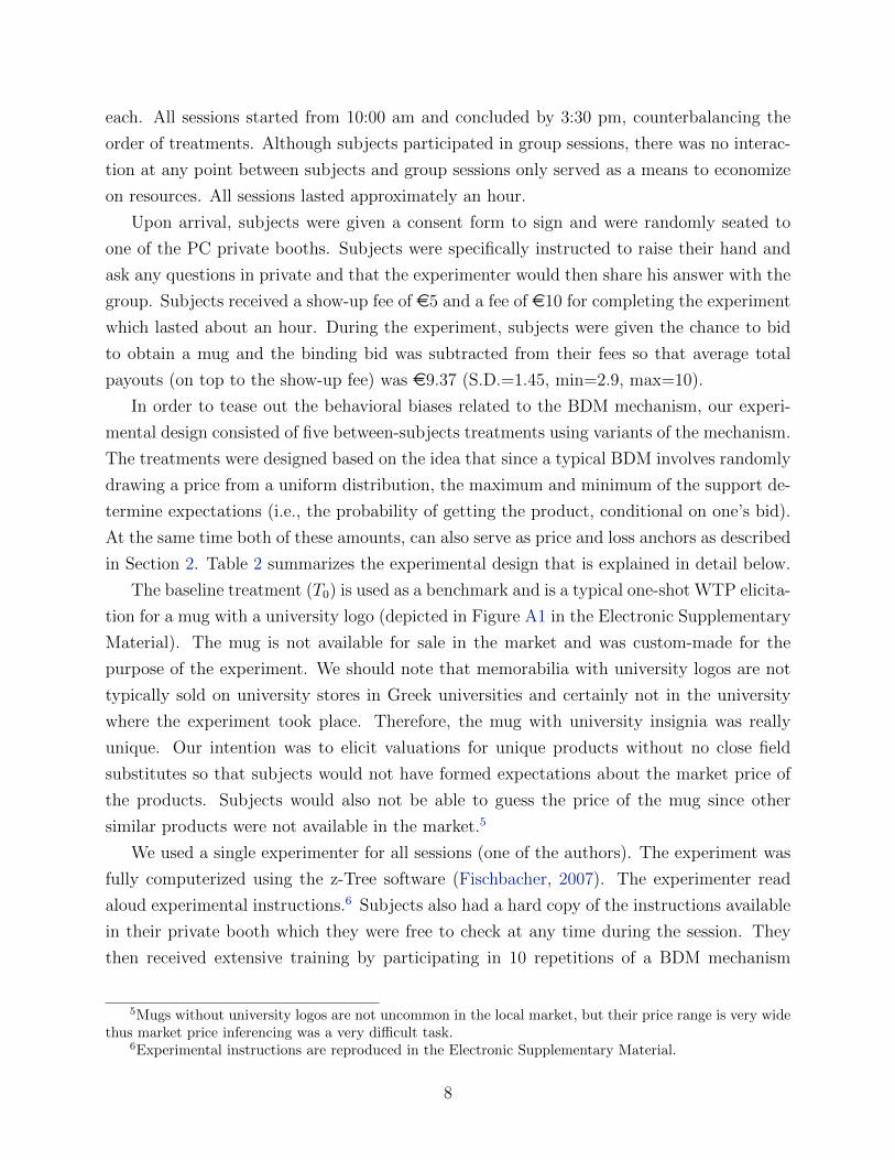
difference of our task to other BDM procedures was that in addition to letting subjects freely

type their bid, we used an interface where subjects had to scroll a slide bar between 0 and

15 Euros (see figure 1 below).7

Figure 1: Bidding screen

Upon sliding the bar horizontally, at any point between or at the two sides, subjects were

given a number of relevant information: 1) the bid amount corresponding to the current

point where the bar was released 2) the probability of leaving the session with the mug (as

part of the instructions, the experimenter explained how the objective probabilities were

calculated in detail; see Experimental Instructions) and 3) the highest price they could pay

for the mug if they were to submit this bid. We presented this information to subjects

having in mind Ratan (2015) who showed that such information alone is unlikely to affect

subjects’ bids. Subjects also had the opportunity to move the bar by typing their bid, if they

7The monetary interval of the bar was kept constant across all treatments. To avoid uncontrolledanchoring effects, the starting point of the bar was set to zero.

9

wished to do so. Most importantly, as mentioned before, in order to facilitate decoupling

of expectations about the outcome with price anchors, the binding price was determined

by a random draw of a set of 60 numbers (1-60) and not prices; each of the sixty numbers

corresponded to a price in the following fashion: {1, 2, . . . , 59, 60} → {e0.1, e0.2, . . . , 5.9,

e6.0} (see Table A1 in the Electronic Supplementary Material). We included a similar table

in the experimental instructions mapping numbers to prices, which subjects could refer to

at any point during the experiment.

The first two treatments (T1 and TEL0 )were designed to test whether subjects’ behaviors

can be explained by standard preferences or whether subjects exhibit signs of loss aversion,

and if loss aversion is at play, whether the status-quo or expectations are more likely to act

as the respective reference points.

The T1 treatment was designed to manipulate expectations in a way that would not affect

price and loss anchors. The only difference between T1 and the baseline treatment T0 was that

60 more numbers were added to the virtual urn in T1 (thus, the random draw was between

numbers 1-120). The sixty extra number corresponded to a price of 6 euros (see Table A2 in

the Electronic Supplementary Material), so the new number to price correspondence followed

the following fashion: {1, 2, . . . , 59, 60, 61 . . . 119, 120} → {e0.1, e0.2, . . . , e5.9, e6.0,

e6.0 . . . , e6.0, e6.0 }. Thus, adding the numbers had no effect the range of possible prices

of the mug (the price of the mug was still expected to be somewhere between e0.1 and e6,

as in T0) but it did affect the probability of price realizations: with 50% probability the price

would be between e0.1 and e6 and with 50% probability it would be e6. Notice that the

loss anchor should not be affected by treatment T1 since the maximum loss that a subject

could incur during the experiment is still e6. Similarly, the price anchor is also not affected,

since the minimum and maximum price a subject could purchase the mug is e0.1 and e6,

respectively. However, as long as expectations are not expected to double one’s equilibrium

bid given her true value (but rather to slightly decrease it, see Banerji and Gupta, 2014),

treatment T1 decreases the probability of leaving the experiment with the mug for any value

with an interior solution in T0 (i.e., between e0 and e6). Heidhues and Koszegi (2014)

show how this weakened ‘attachment effect’ is expected to drive bids into lower levels under

the Koszegi and Rabin (2006) framework. Thus, expectations-based preferences would be

supported by a negative treatment effect in T1 when compared to T0. On the other hand,

the absence of a treatment effect would lead to rejection of this preference structure but

would fail to distinguish between rational agents in the neoclassical sense and agents with

reference-dependent preferences whose reference points are formed by the status-quo and not

their expectations.

To avoid a failure of distinguishing between rational agents and agents with reference-

10

dependent preferences, we designed the Equivalent Loss treatment (TEL0 ). The TEL

0 treat-

ment was again identical to the baseline treatment T0, with the exception that instead of

subjects bidding to acquire a mug, they bid to avoid returning the piece of mug they have

been endowed with at the beginning of the session. If reference points are formed by current

status (i.e., having the mug) and subjects are loss averse, leaving the session without the

mug would be considered a loss. Thus, the WTP and EL measures are expected to differ

(see also Bateman et al., 1997). On the other hand, since expected utility for each bid is not

affected by framing under EUT, the WTP and EL measures of value should be equal under

this framework. This would be the case as well, if bidders are loss-averse but expectations

rather than the status-quo act as reference points. This is because the probability of leaving

the experiment with the mug given a subject’s bid is the same for both the TEL0 and the T0

treatments, so expectations are not affected.

In essence, the TEL0 treatment will reveal whether a null effect in T1 is due to expectations

acting as reference points or due to reference-dependent preferences in general. In particular,

if we do not detect any treatment effect in T1 and we also find a null effect in TEL0 , the

neoclassical preference structure cannot be rejected; on the contrary, if the treatment effect

in TEL0 is not null while the T1 treatment effect is null, then the concept of reference-

dependence would not be rejected, but expectations cannot be considered a valid reference

point. In case that a non-null effect is detected in T1, then TEL0 becomes a test of the no-

loss-in-buying (NLIB) hypothesis of Novemsky and Kahneman (2005). To understand why

this is the case, remember that expectations (and, thus, reference points) are the same under

both valuation formats (i.e., WTP and EL). However, if the NLIB hypothesis is true, then

in the probability space that trading is expected, money given to buy the mug would not

be treated as a loss in the WTP treatment. Thus, the respective states are not weighted by

the loss aversion coefficient in the expected utility of the decision-makers as the feeling of

loss is outweighed by that of a gain (i.e. getting the mug). Under the EL framing however,

subjects do perceive money given in the same states as losses, since money are given to avoid

losing the product and not to buy it (buying the product would feel like a gain). Table 1

summarizes the hypotheses that would be supported given null or non-null treatment effects

for the T1 and TEL0 treatments.

Treatment T2 was designed to reveal price anchoring effects, if any. T2 is similar to T1

(we use the same 120-number virtual urn), but this time the (60) numbers that corresponded

to six-euros prices in T1 now corresponded to prices in the e6-e12 continuum, so that the

mapping of numbers to prices was as follows: {1, 2, . . . , 59, 60, 61 . . . 119, 120} → {0.1e,

0.2e, . . . , 5.9e, 6.0e, 6.1e, . . . , 11.9e, 12.0e} (see Table A3). As a result, expected

outcomes, remain unaffected between treatments T2 and T1 for bids up to e6. To keep

11

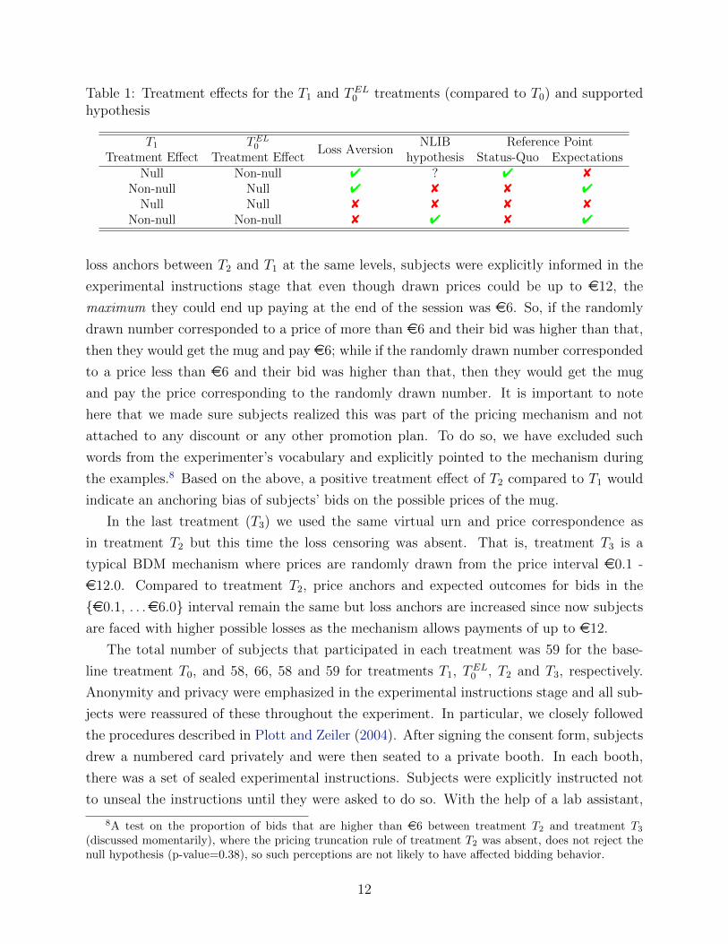
Table 1: Treatment effects for the T1 and TEL0 treatments (compared to T0) and supported

hypothesis

T1

Treatment EffectTEL0

Treatment EffectLoss Aversion

NLIBhypothesis

Reference PointStatus-Quo Expectations

Null Non-null 4 ? 4 8

Non-null Null 4 8 8 4

Null Null 8 8 8 8

Non-null Non-null 8 4 8 4

loss anchors between T2 and T1 at the same levels, subjects were explicitly informed in the

experimental instructions stage that even though drawn prices could be up to e12, the

maximum they could end up paying at the end of the session was e6. So, if the randomly

drawn number corresponded to a price of more than e6 and their bid was higher than that,

then they would get the mug and pay e6; while if the randomly drawn number corresponded

to a price less than e6 and their bid was higher than that, then they would get the mug

and pay the price corresponding to the randomly drawn number. It is important to note

here that we made sure subjects realized this was part of the pricing mechanism and not

attached to any discount or any other promotion plan. To do so, we have excluded such

words from the experimenter’s vocabulary and explicitly pointed to the mechanism during

the examples.8 Based on the above, a positive treatment effect of T2 compared to T1 would

indicate an anchoring bias of subjects’ bids on the possible prices of the mug.

In the last treatment (T3) we used the same virtual urn and price correspondence as

in treatment T2 but this time the loss censoring was absent. That is, treatment T3 is a

typical BDM mechanism where prices are randomly drawn from the price interval e0.1 -

e12.0. Compared to treatment T2, price anchors and expected outcomes for bids in the

{e0.1, . . .e6.0} interval remain the same but loss anchors are increased since now subjects

are faced with higher possible losses as the mechanism allows payments of up to e12.

The total number of subjects that participated in each treatment was 59 for the base-

line treatment T0, and 58, 66, 58 and 59 for treatments T1, TEL0 , T2 and T3, respectively.

Anonymity and privacy were emphasized in the experimental instructions stage and all sub-

jects were reassured of these throughout the experiment. In particular, we closely followed

the procedures described in Plott and Zeiler (2004). After signing the consent form, subjects

drew a numbered card privately and were then seated to a private booth. In each booth,

there was a set of sealed experimental instructions. Subjects were explicitly instructed not

to unseal the instructions until they were asked to do so. With the help of a lab assistant,

8A test on the proportion of bids that are higher than e6 between treatment T2 and treatment T3(discussed momentarily), where the pricing truncation rule of treatment T2 was absent, does not reject thenull hypothesis (p-value=0.38), so such perceptions are not likely to have affected bidding behavior.

12

they input their ID number to a field shown in their computer screen; this number was their

ID for the rest of the session.

At the end of each session and while subjects completed the accompanying questionnaire,

the experimenter calculated the amount of money the subjects should receive (i.e., subtract-

ing from their fees any payment for the mug) and checked whether they were entitled to get

a mug or not. For each subject ID, the experimenter sealed the corresponding amount into

an envelop that had the specific number printed on the outside and also compiled a new list

with the set of IDs that should receive a mug. Both the envelop and the list were given to

another lab assistant that passed them on to a third lab assistant located in another building

in the campus, just a few meters away from the lab location. The third lab assistant who

received the envelop and the list was instructed to give the envelops and mugs based on the

card numbers subjects were holding and was completely unaware of any other details regard-

ing the experiment. Therefore, after the session was over, subjects simply left the computer

lab holding their ID cards and then walked to the other building to exchange it with the

corresponding envelop with their earnings and possibly (depending on the outcome of the

experiment) a mug. In the instructions, we also avoided using strong words such as ‘buy’,

‘it’s yours’, ‘you own’ etc. that could potentially affect the behavior of the participants.

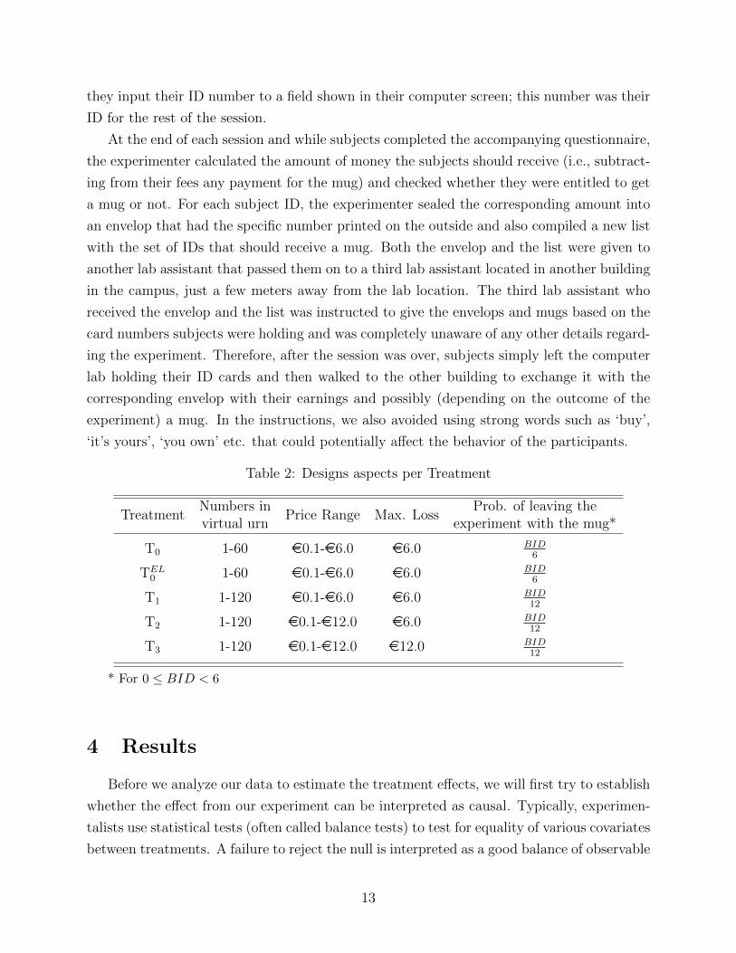
Table 2: Designs aspects per Treatment

TreatmentNumbers invirtual urn

Price Range Max. LossProb. of leaving the

experiment with the mug*

T0 1-60 e0.1-e6.0 e6.0 BID6

TEL0 1-60 e0.1-e6.0 e6.0 BID

6

T1 1-120 e0.1-e6.0 e6.0 BID12

T2 1-120 e0.1-e12.0 e6.0 BID12

T3 1-120 e0.1-e12.0 e12.0 BID12

* For 0 ≤ BID < 6

4 Results

Before we analyze our data to estimate the treatment effects, we will first try to establish

whether the effect from our experiment can be interpreted as causal. Typically, experimen-

talists use statistical tests (often called balance tests) to test for equality of various covariates

between treatments. A failure to reject the null is interpreted as a good balance of observable

13

characteristics between treatments and a success of the randomization process. Briz et al.

(2017) provide a detailed discussion about the literature that points to the pitfalls of using

balance tests (e.g., Deaton and Cartwright, 2017; Ho et al., 2007; Moher et al., 2010; Mutz

and Pemantle, 2015). Following Deaton and Cartwright’s (2017) advice, we report instead

the standardized difference in means (Imbens and Rubin, 2016; Imbens and Wooldridge,

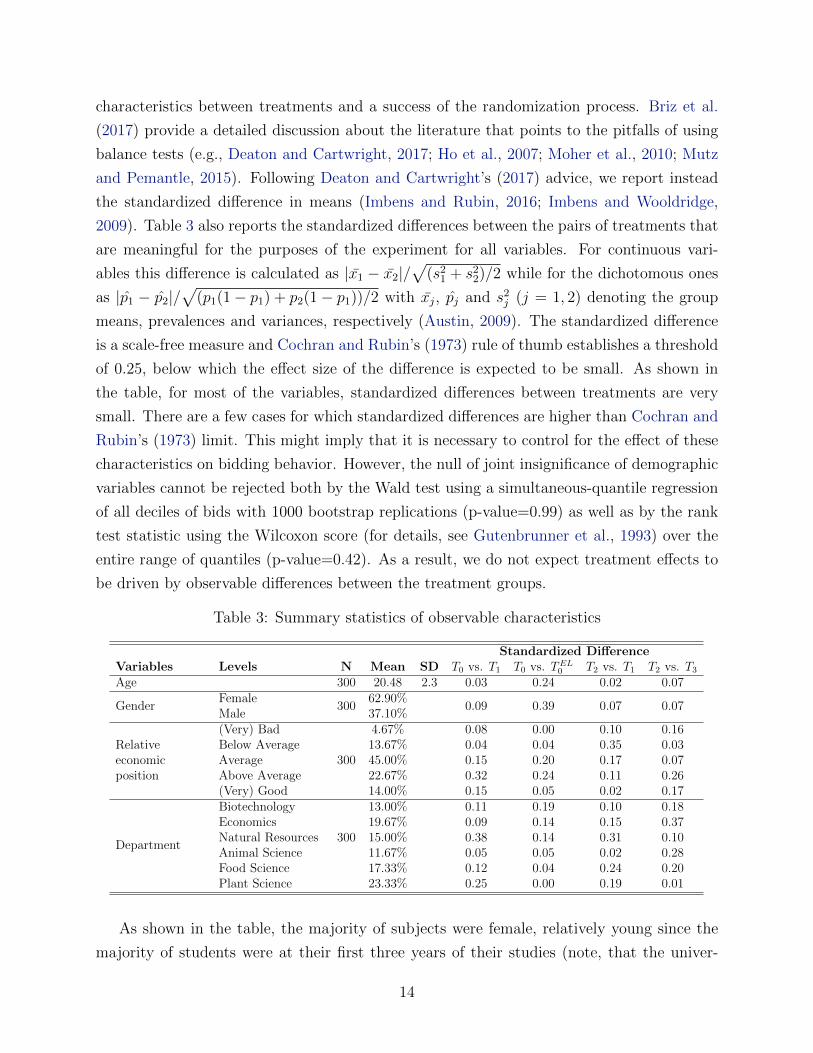
2009). Table 3 also reports the standardized differences between the pairs of treatments that

are meaningful for the purposes of the experiment for all variables. For continuous vari-

ables this difference is calculated as |x1 − x2|/√

(s21 + s22)/2 while for the dichotomous ones

as |p1 − p2|/√

(p1(1− p1) + p2(1− p1))/2 with xj, pj and s2j (j = 1, 2) denoting the group

means, prevalences and variances, respectively (Austin, 2009). The standardized difference

is a scale-free measure and Cochran and Rubin’s (1973) rule of thumb establishes a threshold

of 0.25, below which the effect size of the difference is expected to be small. As shown in

the table, for most of the variables, standardized differences between treatments are very

small. There are a few cases for which standardized differences are higher than Cochran and

Rubin’s (1973) limit. This might imply that it is necessary to control for the effect of these

characteristics on bidding behavior. However, the null of joint insignificance of demographic

variables cannot be rejected both by the Wald test using a simultaneous-quantile regression

of all deciles of bids with 1000 bootstrap replications (p-value=0.99) as well as by the rank

test statistic using the Wilcoxon score (for details, see Gutenbrunner et al., 1993) over the

entire range of quantiles (p-value=0.42). As a result, we do not expect treatment effects to

be driven by observable differences between the treatment groups.

Table 3: Summary statistics of observable characteristics

Standardized DifferenceVariables Levels N Mean SD T0 vs. T1 T0 vs. TEL

0 T2 vs. T1 T2 vs. T3

Age 300 20.48 2.3 0.03 0.24 0.02 0.07

GenderFemale

30062.90%

0.09 0.39 0.07 0.07Male 37.10%

Relativeeconomicposition

(Very) Bad

300

4.67% 0.08 0.00 0.10 0.16Below Average 13.67% 0.04 0.04 0.35 0.03Average 45.00% 0.15 0.20 0.17 0.07Above Average 22.67% 0.32 0.24 0.11 0.26(Very) Good 14.00% 0.15 0.05 0.02 0.17

Department

Biotechnology

300

13.00% 0.11 0.19 0.10 0.18Economics 19.67% 0.09 0.14 0.15 0.37Natural Resources 15.00% 0.38 0.14 0.31 0.10Animal Science 11.67% 0.05 0.05 0.02 0.28Food Science 17.33% 0.12 0.04 0.24 0.20Plant Science 23.33% 0.25 0.00 0.19 0.01

As shown in the table, the majority of subjects were female, relatively young since the

majority of students were at their first three years of their studies (note, that the univer-

14

sity offers a 5-year bachelor degree), of average relative income, and split between the six

departments of the university in proportion to the size of the population of each department.

In order to avoid artificial differences in the analysis of bidding behavior induced by

our experimental design (recall that some treatments implemented a price support of {e0.1

. . . , e6.0} while others a support of {e0.1 . . . , e12.0}) and to standardize the analysis

across treatments, we censored all bids higher than e6 (15 observations in total or 5% of all

observations) to a value of e6 (i.e., these observations were recoded as e6).9 We proceed

in this manner because it is the only way to have comparable bids among all treatments

since, by design, in treatments T0, TEL0 , T1 and T2, bids that are higher than e6 have no

quantitative meaning and are only indicative of a valuation that is higher than e6. To

understand why, remember that the highest possible price in T0, T1 was e6, so bidding

anything above that price yields the same probability of leaving the experiment with the

mug (i.e. 100%) and the same expected payment conditional on buying as bidding e6 (i.e.,

bid/2). For T2, the expected utility from any bid (b) that is higher than e6 is 12

(u (m)− 3)+∫ b

6(u (m)− 6) f(p) dp, with u(m) denoting the utility associated with getting the mug. It

is obvious that increasing one’s bid to the highest price maximizes this utility; the same

argument can be made for reference-dependent expected utility with status-quo acting as

the reference point. For expectations-based reference-dependent expected utility maximizers,

the benefit of increasing one’s bid is not only the maximization of the utility part associated

with the expected gain from getting the mug at the price of e6, but also minimization of

one’s (dis)utility associated with the loss sensation attached to not getting the mug when

she expects to do so.

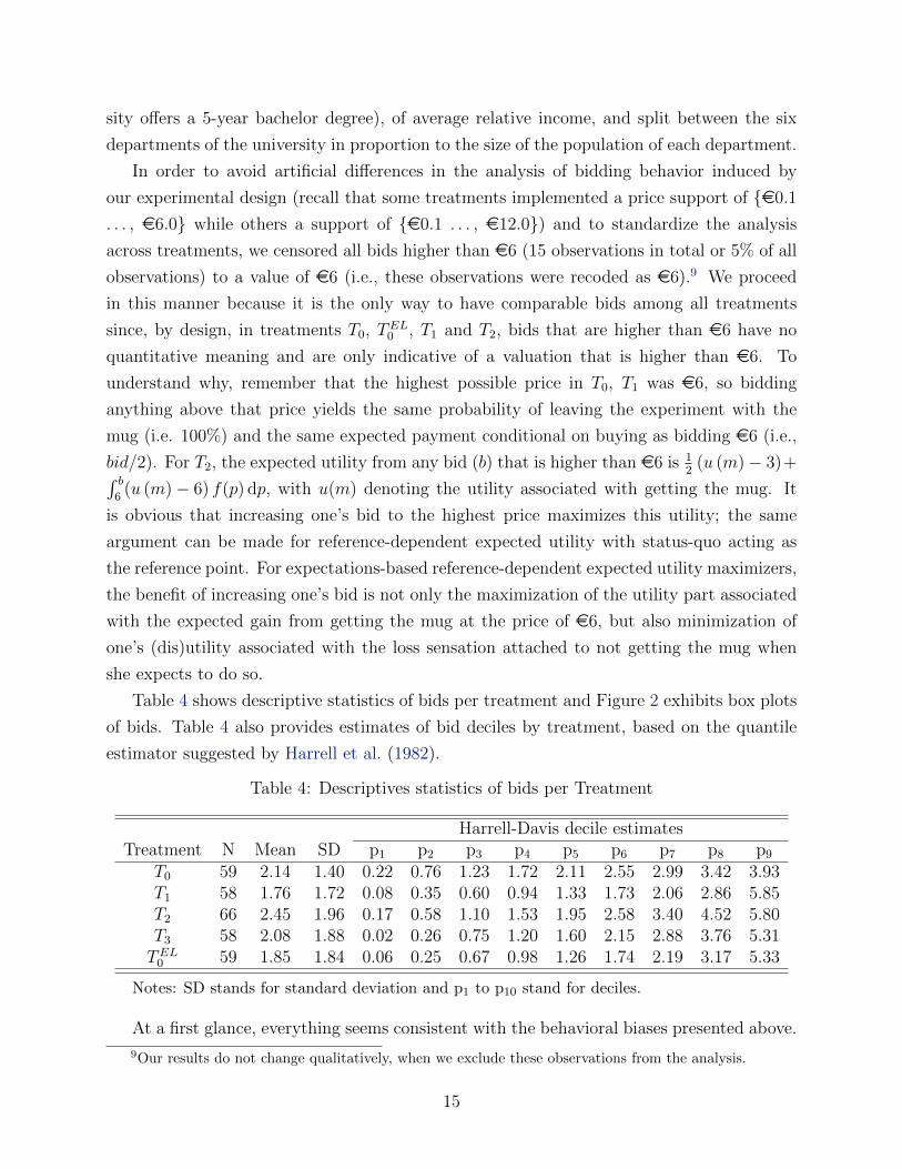
Table 4 shows descriptive statistics of bids per treatment and Figure 2 exhibits box plots

of bids. Table 4 also provides estimates of bid deciles by treatment, based on the quantile

estimator suggested by Harrell et al. (1982).

Table 4: Descriptives statistics of bids per Treatment

Harrell-Davis decile estimatesTreatment N Mean SD p1 p2 p3 p4 p5 p6 p7 p8 p9

T0 59 2.14 1.40 0.22 0.76 1.23 1.72 2.11 2.55 2.99 3.42 3.93T1 58 1.76 1.72 0.08 0.35 0.60 0.94 1.33 1.73 2.06 2.86 5.85T2 66 2.45 1.96 0.17 0.58 1.10 1.53 1.95 2.58 3.40 4.52 5.80T3 58 2.08 1.88 0.02 0.26 0.75 1.20 1.60 2.15 2.88 3.76 5.31TEL0 59 1.85 1.84 0.06 0.25 0.67 0.98 1.26 1.74 2.19 3.17 5.33

Notes: SD stands for standard deviation and p1 to p10 stand for deciles.

At a first glance, everything seems consistent with the behavioral biases presented above.

9Our results do not change qualitatively, when we exclude these observations from the analysis.

15

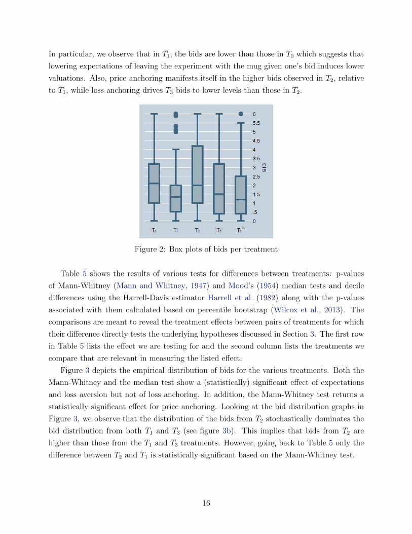
In particular, we observe that in T1, the bids are lower than those in T0 which suggests that

lowering expectations of leaving the experiment with the mug given one’s bid induces lower

valuations. Also, price anchoring manifests itself in the higher bids observed in T2, relative

to T1, while loss anchoring drives T3 bids to lower levels than those in T2.

Figure 2: Box plots of bids per treatment

Table 5 shows the results of various tests for differences between treatments: p-values

of Mann-Whitney (Mann and Whitney, 1947) and Mood’s (1954) median tests and decile

differences using the Harrell-Davis estimator Harrell et al. (1982) along with the p-values

associated with them calculated based on percentile bootstrap (Wilcox et al., 2013). The

comparisons are meant to reveal the treatment effects between pairs of treatments for which

their difference directly tests the underlying hypotheses discussed in Section 3. The first row

in Table 5 lists the effect we are testing for and the second column lists the treatments we

compare that are relevant in measuring the listed effect.

Figure 3 depicts the empirical distribution of bids for the various treatments. Both the

Mann-Whitney and the median test show a (statistically) significant effect of expectations

and loss aversion but not of loss anchoring. In addition, the Mann-Whitney test returns a

statistically significant effect for price anchoring. Looking at the bid distribution graphs in

Figure 3, we observe that the distribution of the bids from T2 stochastically dominates the

bid distribution from both T1 and T3 (see figure 3b). This implies that bids from T2 are

higher than those from the T1 and T3 treatments. However, going back to Table 5 only the

difference between T2 and T1 is statistically significant based on the Mann-Whitney test.

16

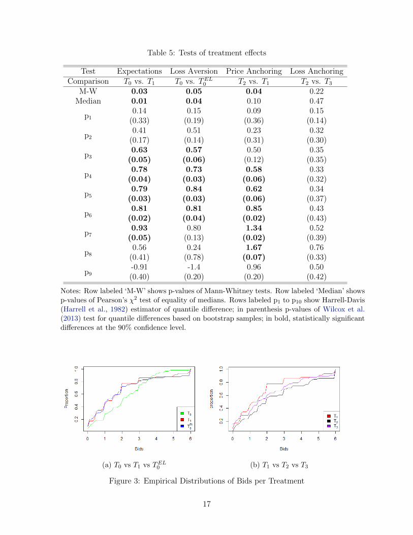
Table 5: Tests of treatment effects

Test Expectations Loss Aversion Price Anchoring Loss AnchoringComparison T0 vs. T1 T0 vs. TEL

0 T2 vs. T1 T2 vs. T3

M-W 0.03 0.05 0.04 0.22Median 0.01 0.04 0.10 0.47

p10.14

(0.33)0.15

(0.19)0.09

(0.36)0.15

(0.14)

p20.41

(0.17)0.51

(0.14)0.23

(0.31)0.32

(0.30)

p30.63

(0.05)0.57

(0.06)0.50

(0.12)0.35

(0.35)

p40.78

(0.04)0.73

(0.03)0.58

(0.06)0.33

(0.32)

p50.79

(0.03)0.84

(0.03)0.62

(0.06)0.34

(0.37)

p60.81

(0.02)0.81

(0.04)0.85

(0.02)0.43

(0.43)

p70.93

(0.05)0.80

(0.13)1.34

(0.02)0.52

(0.39)

p80.56

(0.41)0.24

(0.78)1.67

(0.07)0.76

(0.33)

p9-0.91(0.40)

-1.4(0.20)

0.96(0.20)

0.50(0.42)

Notes: Row labeled ‘M-W’ shows p-values of Mann-Whitney tests. Row labeled ‘Median’ showsp-values of Pearson’s χ2 test of equality of medians. Rows labeled p1 to p10 show Harrell-Davis(Harrell et al., 1982) estimator of quantile difference; in parenthesis p-values of Wilcox et al.(2013) test for quantile differences based on bootstrap samples; in bold, statistically significantdifferences at the 90% confidence level.

(a) T0 vs T1 vs TEL0 (b) T1 vs T2 vs T3

Figure 3: Empirical Distributions of Bids per Treatment

17

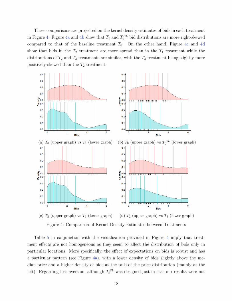
These comparisons are projected on the kernel density estimates of bids in each treatment

in Figure 4. Figure 4a and 4b show that T1 and TEL0 bid distributions are more right-skewed

compared to that of the baseline treatment T0. On the other hand, Figure 4c and 4d

show that bids in the T2 treatment are more spread than in the T1 treatment while the

distributions of T2 and T3 treatments are similar, with the T3 treatment being slightly more

positively-skewed than the T2 treatment.

(a) T0 (upper graph) vs T1 (lower graph) (b) T0 (upper graph) vs TEL0 (lower graph)

(c) T2 (upper graph) vs T1 (lower graph) (d) T2 (upper graph) vs T3 (lower graph)

Figure 4: Comparison of Kernel Density Estimates between Treatments

Table 5 in conjunction with the visualization provided in Figure 4 imply that treat-

ment effects are not homogeneous as they seem to affect the distribution of bids only in

particular locations. More specifically, the effect of expectations on bids is robust and has

a particular pattern (see Figure 4a), with a lower density of bids slightly above the me-

dian price and a higher density of bids at the tails of the price distribution (mainly at the

left). Regarding loss aversion, although TEL0 was designed just in case our results were not

18

supportive of expectation-based preferences (as mentioned before, we find significant sup-

port for expectation-based preferences), the treatment yields interesting results by itself (see

Figure 4b). The TEL0 treatment yields a significant treatment effect, similar to that of T1

when compared to the T0 treatment. When comparing T2 vs. T1, we see that T2 has an

effect that is located mainly on the higher quantiles of the bid distribution indicating that

anchoring might have a more profound effect on subjects bidding at the higher end of the

price distribution. Finally, comparison of T2 with T3 reveals a non-statistically significantly

difference.

5 Discussion

The popularity of the BDM mechanism in WTP value elicitation relies on its simplicity

and incentive compatibility under EUT. However, red flags have been raised about the

usefulness of the mechanism given that subjects’ behavior in the BDM has been found to

be driven by several biases that are not included in the EUT paradigm. In this paper,

we attempted to examine a number of these biases, such as reference-dependent preferences,

expectation-based reference points as well as price and loss anchoring. By varying the amount

of numbered labels in a virtual urn and mapping these numbered labels into prices, we were

able to disentangle the effect of these biases on bidding behavior in a way that does not

deviate from the rational of regular BDM experimental tasks. It is also important to note

that we achieved this without having to introduce additional lotteries that would further

challenge the cognitive ability of subjects and might cause misconceptions.

Comparing the full distribution of bids across treatments, we identify various treatment

effects. The T0 vs. T1 treatments show a significant treatment effect which we can attribute

on expectations in the Koszegi and Rabin’s (2006) framework. In addition, this result is not

in line with other competing models of expectation-based preferences, such as the ‘good-deal

model’ of Wenner (2015) or the ‘bad-deal aversion’ model of Isoni (2011). In particular, based

on the ‘good-deal model’ (Wenner, 2015), bids in the T1 treatment should have been higher

than the baseline T0 treatment, since the mug was more ‘expensive’ (in terms of expected

price) in T1 and thus, higher prices should have felt as a better deal to subjects, making them

more acceptable. On the other hand, the ‘bad-deal aversion’ model (Isoni, 2011) assumes

that in the formulation of the reference price, only those prices that consumers are willing to

pay actually matter. In the BDM framework, this corresponds to those prices that are lower

than subject’s bid. Since the reference price or the expected price conditional on buying the

mug for all bids in the {0.1e, 6.0e} interval was the same in both treatments (equal to bid2

),

we should have observed a null treatment effect. Given the above, the only plausible model

19

that is compatible with the treatment effect we observe is that of Koszegi and Rabin (2006).

In reference to the equivalent loss TEL0 treatment, since our results indicate that bids in

TEL0 were different than the baseline T0 treatment and since a non-null effect was detected

in T1 (when compared to T0), the hypothesis that bidders are loss averse (i.e., they dislike

losses relative to a reference point more than they like same-sized gains) cannot be rejected.

However, as described in Section 3 and in Table 1, a pair of non-null treatment effects for

T1 vs. T0 and TEL0 vs. T0 is supportive of the no-loss-in-buying hypothesis of Novemsky and

Kahneman (2005).

Finally, the mechanism of anchoring on the highest possible price was also found to

influence subjects valuations, driving bids to higher levels. In our study, this is manifested by

the observed differences between the bid distributions in treatments T1 and T2. In contrast,

the highest possible loss that could make the utility associated with money more salient,

according to our loss anchoring hypothesis, seems not to influence valuations given that

the observed differences between treatments treatments T2 and T3 were not statistically

significantly different.

Concluding, our results generally indicate that previous research findings that casted

doubts on the incentive compatibility of the BDM mechanism were made on valid ground.

Bids derived from the BDM mechanism are indeed dependent on the underlying distributions

of the random competing bid, due to the expectations they generate and the anchoring of

bids to the chosen price support. Our results also support the no-loss-in-buying hypothesis

of Novemsky and Kahneman (2005) but not the mechanism of loss-anchoring. With regards

to expectations, the behavior we observe is in line with one strand of literature (e.g Banerji

and Gupta, 2014; Marzilli Ericson and Fuster, 2011) that supports the model of Koszegi and

Rabin (2006) but goes against another strand of the literature that is in favor of alterna-

tive theories of distributional dependence (e.g Isoni, 2011; Mazar et al., 2013; Smith, 2012;

Wenner, 2015).

20

References

Austin, P. C. (2009, November). Balance diagnostics for comparing the distribution of base-line covariates between treatment groups in propensity-score matched samples. Statisticsin Medicine 28 (25), 3083–3107.

Banerji, A. and N. Gupta (2014). Detection, identification, and estimation of loss aversion:Evidence from an auction experiment. American Economic Journal: Microeconomics 6 (1),91–133.

Bateman, I., A. Munro, B. Rhodes, C. Starmer, and R. Sugden (1997). A test of the theoryof reference-dependent preferences. Quarterly Journal of Economics 112 (2), 479–505.

Becker, G. M., M. H. DeGroot, and J. Marschak (1964). Measuring utility by a single-response sequential method. Behavioral science 9 (3), 226–232.

Bohm, P., J. Linden, J.n, and J. Sonnegard (1997). Eliciting reservation prices: Becker–degroot–marschak mechanisms vs. markets. The Economic Journal 107 (443), 1079–1089.

Bordalo, P., N. Gennaioli, and A. Shleifer (2012). Salience theory of choice under risk. TheQuarterly Journal of Economics 127 (3), 12431285.

Bordalo, P., N. Gennaioli, and A. Shleifer (2013). Salience and consumer choice. Journal ofPolitical Economy 121 (5), 803–843.

Brewer, N. T. and G. B. Chapman (2002). The fragile basic anchoring effect. Journal ofBehavioral Decision Making 15 (1), 65–77.

Briz, T., A. C. Drichoutis, and R. M. Nayga Jr (2017). Randomization to treatment failurein experimental auctions: The value of data from training rounds. Journal of Behavioraland Experimental Economics 71, 56–66.

Cason, T. N. and C. R. Plott (2014). Misconceptions and game form recognition: Challengesto theoriesof revealed preference and framing. Journal of Political Economy 122 (6), 1235–1270.

Chapman, G. B. and E. J. Johnson (1994). The limits of anchoring. Journal of BehavioralDecision Making 7 (4), 223–242.

Cochran, W. G. and D. B. Rubin (1973). Controlling bias in observational studies: A review.Sankhya: The Indian Journal of Statistics, Series A 35 (4), 417–446.

Deaton, A. and N. Cartwright (2017). Understanding and misunderstanding randomizedcontrolled trials. Social Science & Medicine (In press).

Fischbacher, U. (2007). z-tree: Zurich toolbox for ready-made economic experiments. Ex-perimental Economics 10 (2), 171–178.

Greiner, B. (2015). Subject pool recruitment procedures: Organizing experiments with-ORSEE. Journal of the Economic Science Association 1 (1), 114–125.

21

Gutenbrunner, C., J. Jureckove, R. Koenker, and S. Portnoy (1993). Tests of linear hypothe-ses based on regression rank scores. Journal of Nonparametric Statistics 2 (4), 307–331.

Harrell, F. E., R. M. Califf, D. B. Pryor, K. L. Lee, and R. A. Rosati (1982). Evaluating theyield of medical tests. JAMA: The Journal of the American Medical Association 247 (18),2543–2546.

Heidhues, P. and B. Koszegi (2014, January). Regular prices and sales. Theoretical Eco-nomics 9 (1), 217–251.

Ho, D. E., K. Imai, G. King, and E. A. Stuart (2007). Matching as nonparametric preprocess-ing for reducing model dependence in parametric causal inference. Political Analysis 15 (3),199–236.

Horowitz, J. K. (2006). The becker-degroot-marschak mechanism is not necessarily incentivecompatible, even for non-random goods. Economics Letters 93 (1), 6–11.

Imbens, G. W. and D. B. Rubin (2016). Causal Inference for Statistics, Social, and Biomed-ical Sciences, An introduction. Cambridge and New York: Cambridge University Press.

Imbens, G. W. and J. M. Wooldridge (2009). Recent developments in the econometrics ofprogram evaluation. Journal of Economic Literature 47 (1), 5–86.

Isoni, A. (2011). The willingness-to-accept/willingness-to-pay disparity in repeated markets:loss aversion or ‘bad-deal’ aversion? Theory and Decision 71 (3), 409–430.

Kahneman, D. and A. Tversky (1979). Prospect theory: An analysis of decision under risk.Econometrica 47 (2), 263–292.

Karni, E. and Z. Safra (1987). “preference reversal” and the observability of preferences byexperimental methods. Econometrica, 675–685.

Koszegi, B. and M. Rabin (2006). A model of reference-dependent preferences. The QuarterlyJournal of Economics 121 (4), 1133–1165.

Koszegi, B. and A. Szeidl (2013). A model of focusing in economic choice. The QuarterlyJournal of Economics 128 (1), 53–104.

Mann, H. B. and D. R. Whitney (1947). On a test of whether one of two random variables isstochastically larger than the other. The Annals of Mathematical Statistics 18 (1), 50–60.

Marzilli Ericson, K. M. and A. Fuster (2011). Expectations as endowments: Evidence onreference-dependent preferences from exchange and valuation experiments. The QuarterlyJournal of Economics , 1–29.

Mazar, N. and D. Ariely (2006). Dishonesty in everyday life and its policy implications.Journal of Public Policy & Marketing 25 (1), 117–126.

Mazar, N., B. Koszegi, and D. Ariely (2013). True context-dependent preferences? thecauses of market-dependent valuations. Journal of Behavioral Decision Making .

22

Moher, D., S. Hopewell, K. F. Schulz, V. Montori, P. C. Gtzsche, P. J. Devereaux, D. El-bourne, M. Egger, and D. G. Altman (2010). CONSORT 2010 explanation and elaboration:updated guidelines for reporting parallel group randomised trials. BMJ 340.

Mood, A. M. (1954). On the asymptotic efficiency of certain nonparametric two-sampletests. The Annals of Mathematical Statistics 25 (3), 514–522.

Morewedge, C. K. and D. Kahneman (2010). Associative processes in intuitive judgment.Trends in Cognitive Sciences 14 (10), 435–440.

Mutz, D. C. and R. Pemantle (2015). Standards for experimental research: Encouraginga better understanding of experimental methods. Journal of Experimental Political Sci-ence 2 (2), 192–215.

Novemsky, N. and D. Kahneman (2005). The boundaries of loss aversion. Journal of Mar-keting Research, 119–128.

Plott, C. R. and K. Zeiler (2004). The willingness to pay/willingness to accept gap, theendowment effect, subject misconceptions and experimental procedures for eliciting valu-ations. American Economic Review 95, 530–530.

Plott, C. R. and K. Zeiler (2007). Exchange asymmetries incorrectly interpreted as evidenceof endowment effect theory and prospect theory? The American Economic Review 97 (4),1449–1466.

Ratan, A. (2015). Does displaying probabilities affect bidding in first-price auctions? Eco-nomics Letters 126, 119–121.

Smith, A. (2008). Lagged beliefs and reference-dependent utility. Unpublished paper, Uni-versity of Arizona.

Smith, A. (2012). Lagged beliefs and reference-dependent preferences. working paper, Cali-fornia Institute of Technology .

Sugden, R., J. Zheng, and D. J. Zizzo (2013, December). Not all anchors are created equal.Journal of Economic Psychology 39, 21–31.

Taylor, S. E. and S. C. Thompson (1982). Stalking the elusive ”vividness” effect. Psycho-logical Review 89 (2), 155–181.

Tversky, A. and D. Kahneman (1974). Judgment under uncertainty: Heuristics and biases.Science 185 (4157), 1124–1131.

Tversky, A. and D. Kahneman (1991). Loss aversion in riskless choice: A reference-dependentmodel. The Quarterly Journal of Economics 106 (4), 1039–1039.

Tymula, A., E. Woelbert, and P. Glimcher (2016). Flexible valuations for consumer goodsas measured by the BeckerDeGrootMarschak mechanism. Journal of Neuroscience, Psy-chology, and Economics 9 (2), 65–77.

23

Urbancic, M. (2011). Testing distributional dependence in the becker-degroot-marschakmechanism.

Vickrey, W. (1961). Counterspeculation, auctions, and competitive sealed tenders. TheJournal of Finance 16 (1), 8–37.

Wenner, L. M. (04/2015). Expected prices as reference pointstheory and experiments. Eu-ropean Economic Review 75, 60–79.

Wilcox, R. R., D. M. Erceg-Hurn, F. Clark, and M. Carlson (2013). Comparing two inde-pendent groups via the lower and upper quantiles. Journal of Statistical Computation andSimulation 84 (7), 1543–1551.

Wilson, T. D., C. E. Houston, K. M. Etling, and N. Brekke (1996). A new look at an-choring effects: basic anchoring and its antecedents. Journal of Experimental Psychology:General 125 (4), 387.

24

Electronic Supplementary Material of

Loss Aversion, Expectations, Price and Loss Anchoringin the BDM Mechanism

Achilleas Vassilopoulos∗, Andreas C. Drichoutis† and Rodolfo M. Nayga, Jr.‡

Experimental Instructions

[This is a translation of the original instructions written in Greek. Instructions were providedin hard copies and each box represents a separate page in the instructions. Differences ininstructions between treatments are shown in different color and are included in squarebrackets. A prefix (T0, T1, T

EL0 , T2, T3) indicates that a specific part of the text was only

included in the treatment indicated by the prefix. Explanatory text for the reader is alsocolored and included in square brackets.]

Welcome!

Thank you for agreeing to participate in a survey of how people make decisions. Please readcarefully the instructions given below.

There are no right and wrong answers to any of the questions you will answer, we just wantto know your opinion.

It is very important to follow the instructions carefully. Also, it is very important not tocommunicate with other participants. If you have any questions at any stage of theexperiment, please raise your hand and the experimenter will answer to you in private.

∗Corresponding author: Senior Researcher, International Centre for Research on the Environment andthe Economy, Artemidos 6 & Epidavrou, 15125, Maroussi-Athens, Greece and Department of Agricul-tural Economics & Rural Development, Agricultural University of Athens, tel:+30-210-6875346, e-mail:avas@aua.gr, achilleas.vassilopoulos@icre8.eu.

†Assistant professor, Department of Agricultural Economics & Rural Development, Agricultural Univer-sity of Athens, Iera Odos 75, 11855, Greece, tel: +30-210-5294781, e-mail: adrihout@aua.gr.

‡Distinguished Professor and Tyson Endowed Chair, Department of Agricultural Economics & Agribusi-ness, University of Arkansas, Fayetteville, AR 72701, USA, and NBER, tel:+1-4795752299 e-mail:rnayga@uark.edu.

1

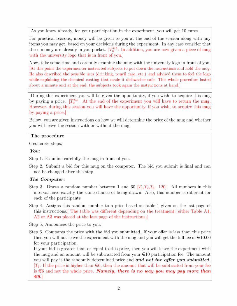
As you know already, for your participation in the experiment, you will get 10 euros.

For practical reasons, money will be given to you at the end of the session along with anyitems you may get, based on your decisions during the experiment. In any case consider thatthese money are already in you pocket. [TEL

0 : In addition, you are now given a piece of mugwith the university logo that is in front of you.]

Now, take some time and carefully examine the mug with the university logo in front of you.[At this point the experimenter instructed subjects to put down the instructions and hold the mug.

He also described the possible uses (drinking, pencil case, etc.) and advised them to feel the logo

while explaining the chemical coating that made it dishwasher-safe. This whole procedure lasted

about a minute and at the end, the subjects took again the instructions at hand.]

During this experiment you will be given the opportunity, if you wish, to acquire this mugby paying a price. [TEL

0 : At the end of the experiment you will have to return the mug.However, during this session you will have the opportunity, if you wish, to acquire this mugby paying a price.]

Below, you are given instructions on how we will determine the price of the mug and whetheryou will leave the session with or without the mug.

The procedure

6 concrete steps:

You:

Step 1. Examine carefully the mug in front of you.

Step 2. Submit a bid for this mug on the computer. The bid you submit is final and cannot be changed after this step.

The Computer:

Step 3. Draws a random number between 1 and 60 [T1,T2,T3: 120]. All numbers in thisinterval have exactly the same chance of being drawn. Also, this number is different foreach of the participants.

Step 4. Assigns this random number to a price based on table 1 given on the last page ofthis instructions.[ The table was different depending on the treatment: either Table A1,A2 or A3 was placed at the last page of the instructions.]

Step 5. Announces the price to you.

Step 6. Compares the price with the bid you submitted. If your offer is less than this pricethen you will not leave the experiment with the mug and you will get the full fee of e10.00for your participation.If your bid is greater than or equal to this price, then you will leave the experiment withthe mug and an amount will be subtraacted from your e10 participation fee. The amountyou will pay is the randomly determined price and and not the offer you submitted .[T3: If the price is higher than e6, then the amount that will be subtracted from your feeis e6 and not the whole price. Namely, there is no way you may pay more thane6.]

2

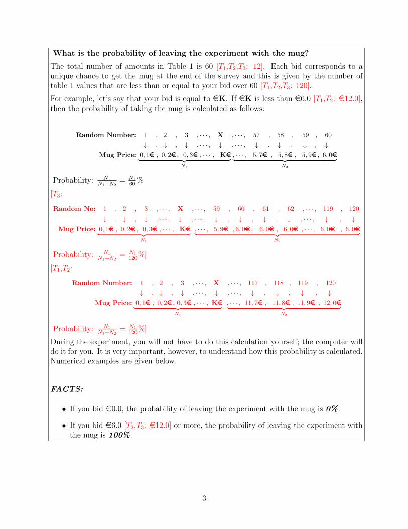
What is the probability of leaving the experiment with the mug?

The total number of amounts in Table 1 is 60 [T1,T2,T3: 12]. Each bid corresponds to aunique chance to get the mug at the end of the survey and this is given by the number oftable 1 values that are less than or equal to your bid over 60 [T1,T2,T3: 120].

For example, let’s say that your bid is equal to eK. If eK is less than e6.0 [T1,T2: e12.0],then the probability of taking the mug is calculated as follows:

Random Number: 1 , 2 , 3 , · · · , X , · · · , 57 , 58 , 59 , 60

↓ , ↓ , ↓ , · · · , ↓ , · · · , ↓ , ↓ , ↓ , ↓Mug Price: 0, 1e , 0, 2e , 0, 3e , · · · , Ke︸ ︷︷ ︸

N1

, · · · , 5, 7e , 5, 8e , 5, 9e , 6, 0e︸ ︷︷ ︸N2

Probability: N1

N1+N2= N1

60%

[T3:

Random No: 1 , 2 , 3 , · · · , X , · · · , 59 , 60 , 61 , 62 , · · · , 119 , 120

↓ , ↓ , ↓ , · · · , ↓ , · · · , ↓ , ↓ , ↓ , ↓ , · · · , ↓ , ↓Mug Price: 0, 1e , 0, 2e , 0, 3e , · · · , Ke︸ ︷︷ ︸

N1

, · · · , 5, 9e , 6, 0e , 6, 0e , 6, 0e , · · · , 6, 0e , 6, 0e︸ ︷︷ ︸N2

Probability: N1

N1+N2= N1

120%]

[T1,T2:

Random Number: 1 , 2 , 3 , · · · , X , · · · , 117 , 118 , 119 , 120

↓ , ↓ , ↓ , · · · , ↓ , · · · , ↓ , ↓ , ↓ , ↓Mug Price: 0, 1e , 0, 2e , 0, 3e , · · · , Ke︸ ︷︷ ︸

N1

, · · · , 11, 7e , 11, 8e , 11, 9e , 12, 0e︸ ︷︷ ︸N2

Probability: N1

N1+N2= N1

120%]

During the experiment, you will not have to do this calculation yourself; the computer willdo it for you. It is very important, however, to understand how this probability is calculated.Numerical examples are given below.

FACTS:

• If you bid e0.0, the probability of leaving the experiment with the mug is 0% .

• If you bid e6.0 [T2,T3: e12.0] or more, the probability of leaving the experiment withthe mug is 100% .

3

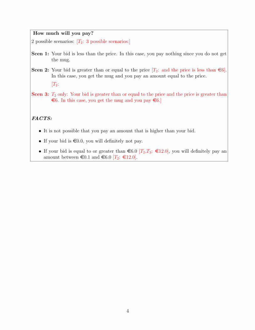
How much will you pay?

2 possible scenarios: [T2: 3 possible scenarios:]

Scen 1: Your bid is less than the price. In this case, you pay nothing since you do not getthe mug.

Scen 2: Your bid is greater than or equal to the price [T2: and the price is less than e6].In this case, you get the mug and you pay an amount equal to the price.

[T2:

Scen 3: T2 only: Your bid is greater than or equal to the price and the price is greater thane6. In this case, you get the mug and you pay e6.]

FACTS:

• It is not possible that you pay an amount that is higher than your bid.

• If your bid is e0.0, you will definitely not pay.

• If your bid is equal to or greater than e6.0 [T2,T3: e12.0], you will definitely pay anamount between e0.1 and e6.0 [T2: e12.0].

4

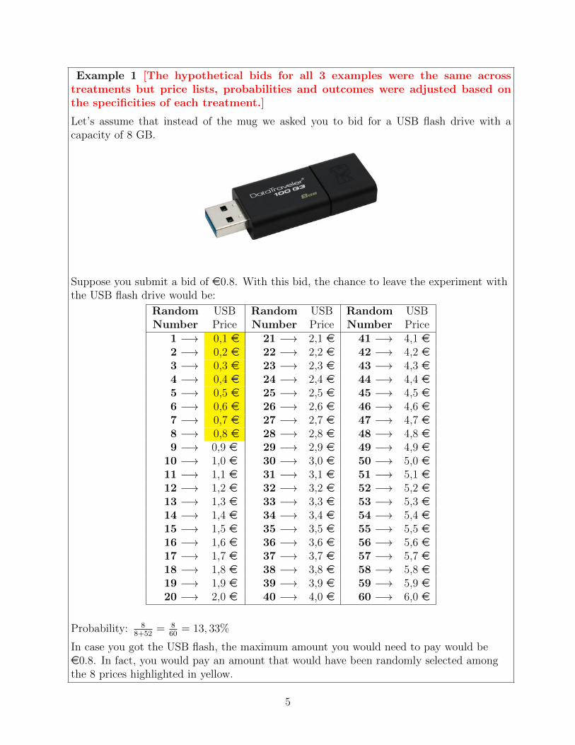
Example 1 [The hypothetical bids for all 3 examples were the same acrosstreatments but price lists, probabilities and outcomes were adjusted based onthe specificities of each treatment.]

Let’s assume that instead of the mug we asked you to bid for a USB flash drive with acapacity of 8 GB.

Suppose you submit a bid of e0.8. With this bid, the chance to leave the experiment withthe USB flash drive would be:

RandomNumber

USBPrice

RandomNumber

USBPrice

RandomNumber

USBPrice

1 −→ 0,1 e 21 −→ 2,1 e 41 −→ 4,1 e2 −→ 0,2 e 22 −→ 2,2 e 42 −→ 4,2 e3 −→ 0,3 e 23 −→ 2,3 e 43 −→ 4,3 e4 −→ 0,4 e 24 −→ 2,4 e 44 −→ 4,4 e5 −→ 0,5 e 25 −→ 2,5 e 45 −→ 4,5 e6 −→ 0,6 e 26 −→ 2,6 e 46 −→ 4,6 e7 −→ 0,7 e 27 −→ 2,7 e 47 −→ 4,7 e8 −→ 0,8 e 28 −→ 2,8 e 48 −→ 4,8 e9 −→ 0,9 e 29 −→ 2,9 e 49 −→ 4,9 e

10 −→ 1,0 e 30 −→ 3,0 e 50 −→ 5,0 e11 −→ 1,1 e 31 −→ 3,1 e 51 −→ 5,1 e12 −→ 1,2 e 32 −→ 3,2 e 52 −→ 5,2 e13 −→ 1,3 e 33 −→ 3,3 e 53 −→ 5,3 e14 −→ 1,4 e 34 −→ 3,4 e 54 −→ 5,4 e15 −→ 1,5 e 35 −→ 3,5 e 55 −→ 5,5 e16 −→ 1,6 e 36 −→ 3,6 e 56 −→ 5,6 e17 −→ 1,7 e 37 −→ 3,7 e 57 −→ 5,7 e18 −→ 1,8 e 38 −→ 3,8 e 58 −→ 5,8 e19 −→ 1,9 e 39 −→ 3,9 e 59 −→ 5,9 e20 −→ 2,0 e 40 −→ 4,0 e 60 −→ 6,0 e

Probability: 88+52

= 860

= 13, 33%

In case you got the USB flash, the maximum amount you would need to pay would bee0.8. In fact, you would pay an amount that would have been randomly selected amongthe 8 prices highlighted in yellow.

5

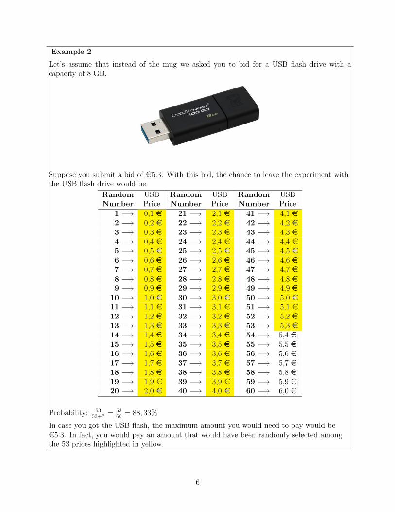
Example 2

Let’s assume that instead of the mug we asked you to bid for a USB flash drive with acapacity of 8 GB.

Suppose you submit a bid of e5.3. With this bid, the chance to leave the experiment withthe USB flash drive would be:

RandomNumber

USBPrice

RandomNumber

USBPrice

RandomNumber

USBPrice

1 −→ 0,1 e 21 −→ 2,1 e 41 −→ 4,1 e2 −→ 0,2 e 22 −→ 2,2 e 42 −→ 4,2 e3 −→ 0,3 e 23 −→ 2,3 e 43 −→ 4,3 e4 −→ 0,4 e 24 −→ 2,4 e 44 −→ 4,4 e5 −→ 0,5 e 25 −→ 2,5 e 45 −→ 4,5 e6 −→ 0,6 e 26 −→ 2,6 e 46 −→ 4,6 e7 −→ 0,7 e 27 −→ 2,7 e 47 −→ 4,7 e8 −→ 0,8 e 28 −→ 2,8 e 48 −→ 4,8 e9 −→ 0,9 e 29 −→ 2,9 e 49 −→ 4,9 e

10 −→ 1,0 e 30 −→ 3,0 e 50 −→ 5,0 e11 −→ 1,1 e 31 −→ 3,1 e 51 −→ 5,1 e12 −→ 1,2 e 32 −→ 3,2 e 52 −→ 5,2 e13 −→ 1,3 e 33 −→ 3,3 e 53 −→ 5,3 e14 −→ 1,4 e 34 −→ 3,4 e 54 −→ 5,4 e15 −→ 1,5 e 35 −→ 3,5 e 55 −→ 5,5 e16 −→ 1,6 e 36 −→ 3,6 e 56 −→ 5,6 e17 −→ 1,7 e 37 −→ 3,7 e 57 −→ 5,7 e18 −→ 1,8 e 38 −→ 3,8 e 58 −→ 5,8 e19 −→ 1,9 e 39 −→ 3,9 e 59 −→ 5,9 e20 −→ 2,0 e 40 −→ 4,0 e 60 −→ 6,0 e

Probability: 5353+7

= 5360

= 88, 33%

In case you got the USB flash, the maximum amount you would need to pay would bee5.3. In fact, you would pay an amount that would have been randomly selected amongthe 53 prices highlighted in yellow.

6

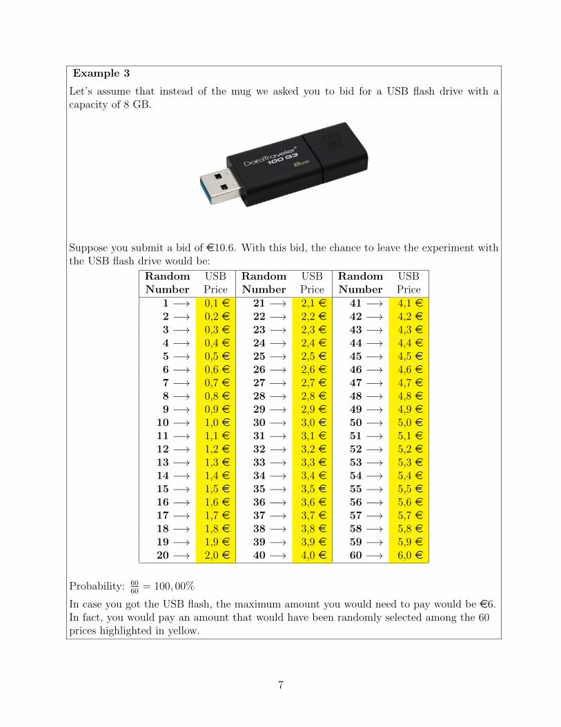
Example 3

Let’s assume that instead of the mug we asked you to bid for a USB flash drive with acapacity of 8 GB.

Suppose you submit a bid of e10.6. With this bid, the chance to leave the experiment withthe USB flash drive would be:

RandomNumber

USBPrice

RandomNumber

USBPrice

RandomNumber

USBPrice

1 −→ 0,1 e 21 −→ 2,1 e 41 −→ 4,1 e2 −→ 0,2 e 22 −→ 2,2 e 42 −→ 4,2 e3 −→ 0,3 e 23 −→ 2,3 e 43 −→ 4,3 e4 −→ 0,4 e 24 −→ 2,4 e 44 −→ 4,4 e5 −→ 0,5 e 25 −→ 2,5 e 45 −→ 4,5 e6 −→ 0,6 e 26 −→ 2,6 e 46 −→ 4,6 e7 −→ 0,7 e 27 −→ 2,7 e 47 −→ 4,7 e8 −→ 0,8 e 28 −→ 2,8 e 48 −→ 4,8 e9 −→ 0,9 e 29 −→ 2,9 e 49 −→ 4,9 e

10 −→ 1,0 e 30 −→ 3,0 e 50 −→ 5,0 e11 −→ 1,1 e 31 −→ 3,1 e 51 −→ 5,1 e12 −→ 1,2 e 32 −→ 3,2 e 52 −→ 5,2 e13 −→ 1,3 e 33 −→ 3,3 e 53 −→ 5,3 e14 −→ 1,4 e 34 −→ 3,4 e 54 −→ 5,4 e15 −→ 1,5 e 35 −→ 3,5 e 55 −→ 5,5 e16 −→ 1,6 e 36 −→ 3,6 e 56 −→ 5,6 e17 −→ 1,7 e 37 −→ 3,7 e 57 −→ 5,7 e18 −→ 1,8 e 38 −→ 3,8 e 58 −→ 5,8 e19 −→ 1,9 e 39 −→ 3,9 e 59 −→ 5,9 e20 −→ 2,0 e 40 −→ 4,0 e 60 −→ 6,0 e

Probability: 6060

= 100, 00%

In case you got the USB flash, the maximum amount you would need to pay would be e6.In fact, you would pay an amount that would have been randomly selected among the 60prices highlighted in yellow.

7

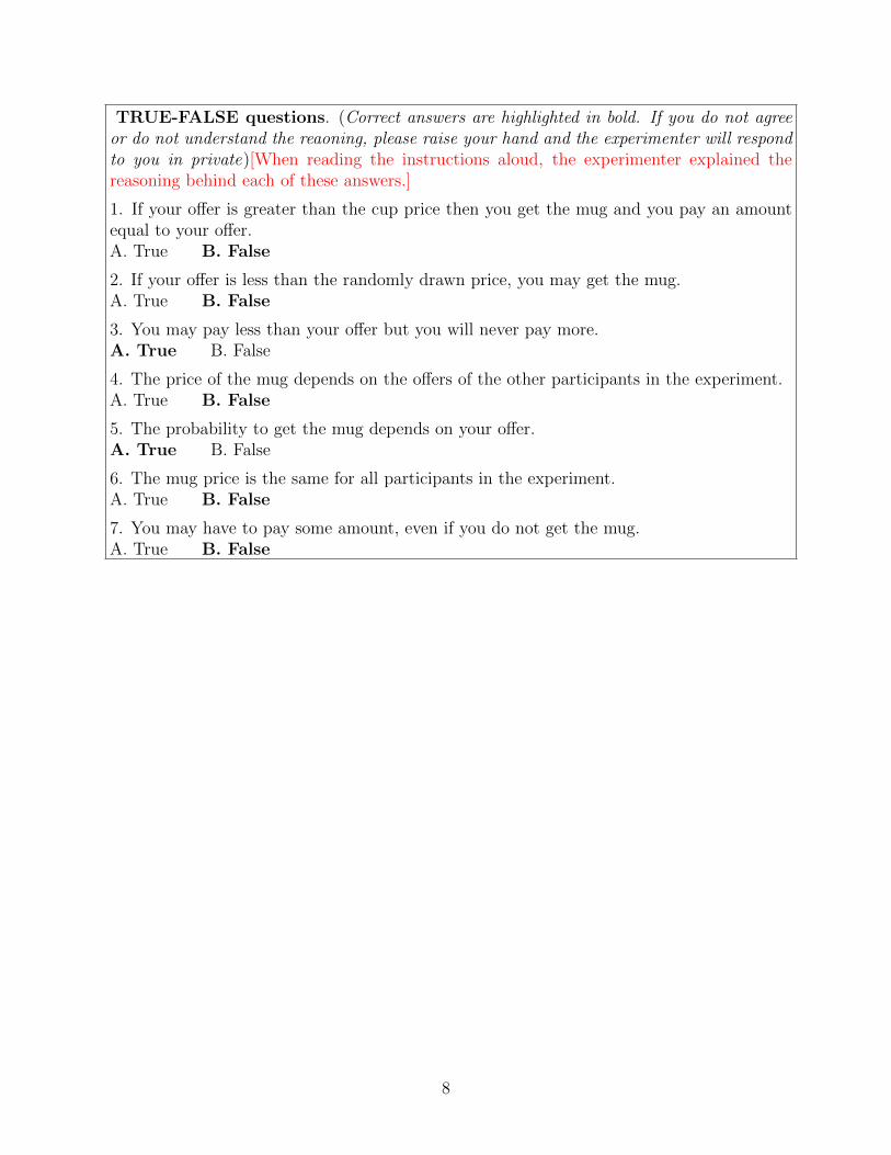
TRUE-FALSE questions. (Correct answers are highlighted in bold. If you do not agreeor do not understand the reaoning, please raise your hand and the experimenter will respondto you in private)[When reading the instructions aloud, the experimenter explained thereasoning behind each of these answers.]

1. If your offer is greater than the cup price then you get the mug and you pay an amountequal to your offer.A. True B. False

2. If your offer is less than the randomly drawn price, you may get the mug.A. True B. False

3. You may pay less than your offer but you will never pay more.A. True B. False

4. The price of the mug depends on the offers of the other participants in the experiment.A. True B. False

5. The probability to get the mug depends on your offer.A. True B. False

6. The mug price is the same for all participants in the experiment.A. True B. False

7. You may have to pay some amount, even if you do not get the mug.A. True B. False

8

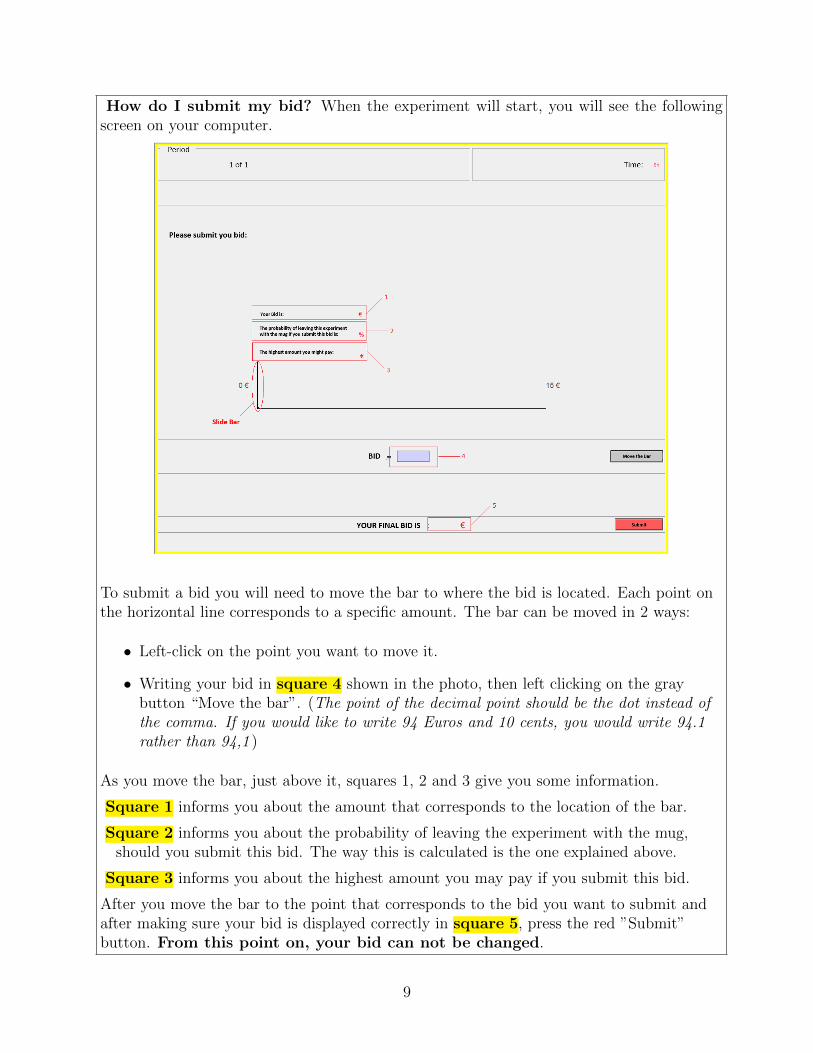
How do I submit my bid? When the experiment will start, you will see the followingscreen on your computer.

To submit a bid you will need to move the bar to where the bid is located. Each point onthe horizontal line corresponds to a specific amount. The bar can be moved in 2 ways:

• Left-click on the point you want to move it.

• Writing your bid in square 4 shown in the photo, then left clicking on the graybutton “Move the bar”. (The point of the decimal point should be the dot instead ofthe comma. If you would like to write 94 Euros and 10 cents, you would write 94.1rather than 94,1 )

As you move the bar, just above it, squares 1, 2 and 3 give you some information.

Square 1 informs you about the amount that corresponds to the location of the bar.

Square 2 informs you about the probability of leaving the experiment with the mug,should you submit this bid. The way this is calculated is the one explained above.

Square 3 informs you about the highest amount you may pay if you submit this bid.

After you move the bar to the point that corresponds to the bid you want to submit andafter making sure your bid is displayed correctly in square 5, press the red ”Submit”button. From this point on, your bid can not be changed.

9

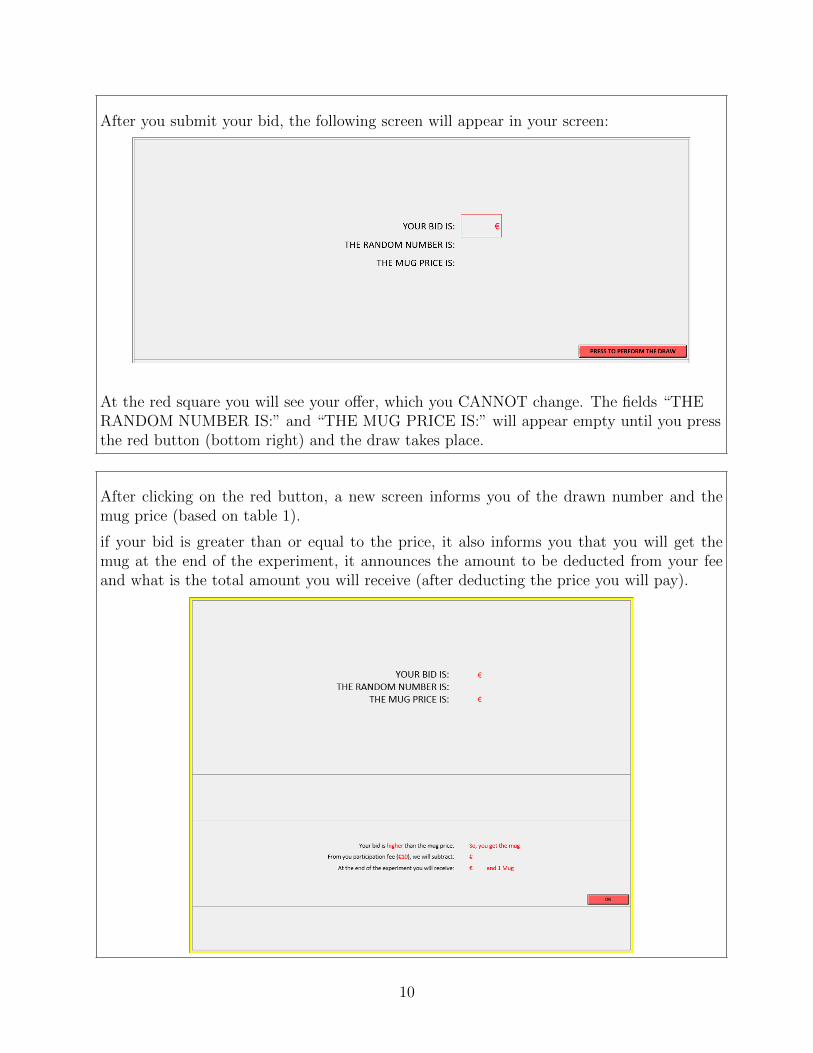
After you submit your bid, the following screen will appear in your screen:

At the red square you will see your offer, which you CANNOT change. The fields “THERANDOM NUMBER IS:” and “THE MUG PRICE IS:” will appear empty until you pressthe red button (bottom right) and the draw takes place.

After clicking on the red button, a new screen informs you of the drawn number and themug price (based on table 1).

if your bid is greater than or equal to the price, it also informs you that you will get themug at the end of the experiment, it announces the amount to be deducted from your feeand what is the total amount you will receive (after deducting the price you will pay).

10

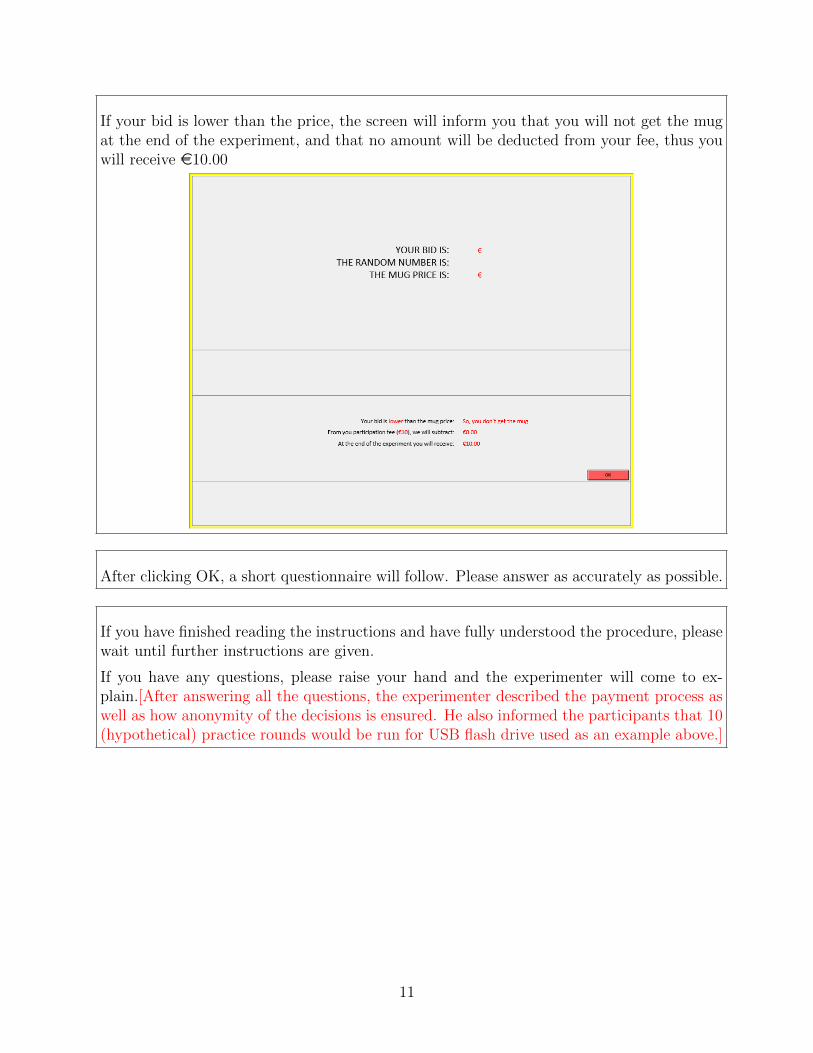
If your bid is lower than the price, the screen will inform you that you will not get the mugat the end of the experiment, and that no amount will be deducted from your fee, thus youwill receive e10.00

After clicking OK, a short questionnaire will follow. Please answer as accurately as possible.

If you have finished reading the instructions and have fully understood the procedure, pleasewait until further instructions are given.

If you have any questions, please raise your hand and the experimenter will come to ex-plain.[After answering all the questions, the experimenter described the payment process aswell as how anonymity of the decisions is ensured. He also informed the participants that 10(hypothetical) practice rounds would be run for USB flash drive used as an example above.]

11

Additional tables and pictures

Figure A1: Mug with university logo

12

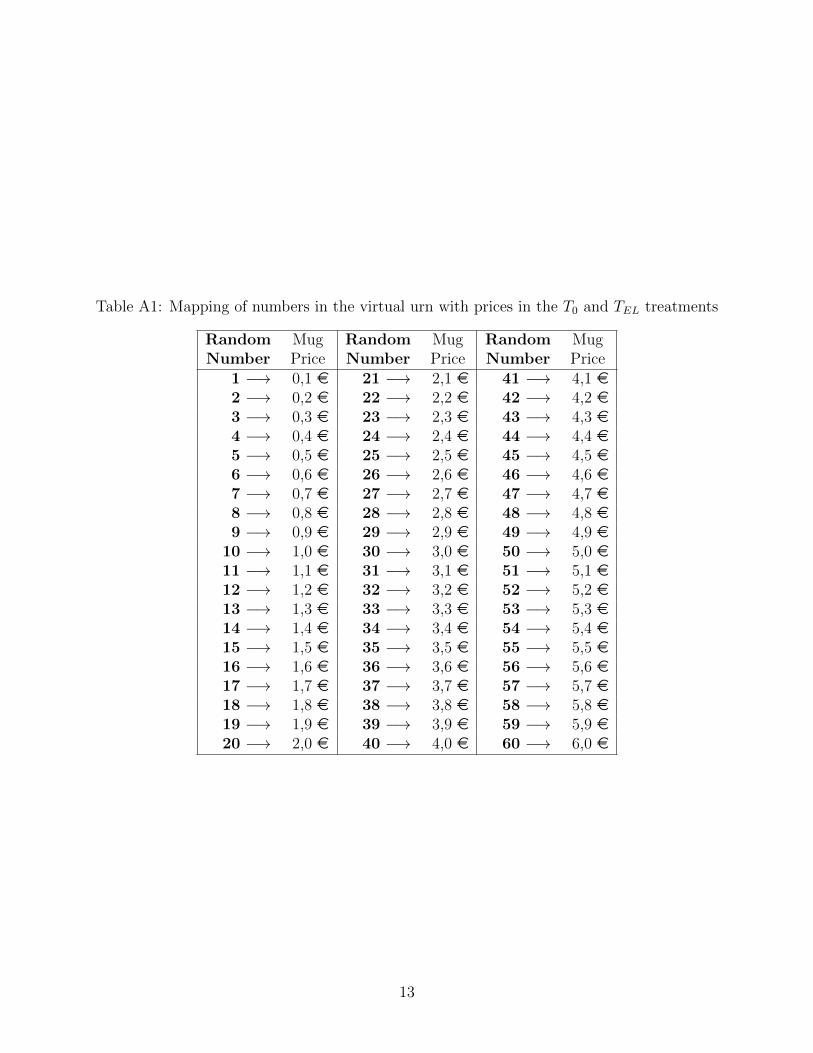
Table A1: Mapping of numbers in the virtual urn with prices in the T0 and TEL treatments

RandomNumber

MugPrice

RandomNumber

MugPrice

RandomNumber

MugPrice

1 −→ 0,1 e 21 −→ 2,1 e 41 −→ 4,1 e2 −→ 0,2 e 22 −→ 2,2 e 42 −→ 4,2 e3 −→ 0,3 e 23 −→ 2,3 e 43 −→ 4,3 e4 −→ 0,4 e 24 −→ 2,4 e 44 −→ 4,4 e5 −→ 0,5 e 25 −→ 2,5 e 45 −→ 4,5 e6 −→ 0,6 e 26 −→ 2,6 e 46 −→ 4,6 e7 −→ 0,7 e 27 −→ 2,7 e 47 −→ 4,7 e8 −→ 0,8 e 28 −→ 2,8 e 48 −→ 4,8 e9 −→ 0,9 e 29 −→ 2,9 e 49 −→ 4,9 e

10 −→ 1,0 e 30 −→ 3,0 e 50 −→ 5,0 e11 −→ 1,1 e 31 −→ 3,1 e 51 −→ 5,1 e12 −→ 1,2 e 32 −→ 3,2 e 52 −→ 5,2 e13 −→ 1,3 e 33 −→ 3,3 e 53 −→ 5,3 e14 −→ 1,4 e 34 −→ 3,4 e 54 −→ 5,4 e15 −→ 1,5 e 35 −→ 3,5 e 55 −→ 5,5 e16 −→ 1,6 e 36 −→ 3,6 e 56 −→ 5,6 e17 −→ 1,7 e 37 −→ 3,7 e 57 −→ 5,7 e18 −→ 1,8 e 38 −→ 3,8 e 58 −→ 5,8 e19 −→ 1,9 e 39 −→ 3,9 e 59 −→ 5,9 e20 −→ 2,0 e 40 −→ 4,0 e 60 −→ 6,0 e

13

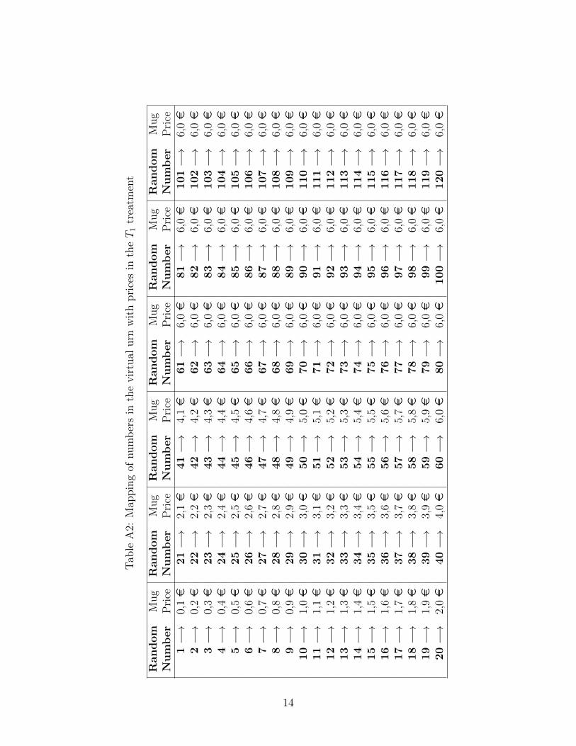
Tab

leA

2:M

appin

gof

num

ber

sin

the

vir

tual

urn

wit

hpri

ces

inth

eT1

trea

tmen

t

Random

Num

ber

Mug

Pri

ceR

andom

Num

ber

Mug

Pri

ceR

andom

Num

ber

Mug

Pri

ceR

andom

Num

ber

Mug

Pri

ceR

andom

Num

ber

Mug

Pri

ceR

andom

Num

ber

Mug

Pri

ce1−→

0,1e

21−→

2,1e

41−→

4,1e

61−→

6,0e

81−→

6,0e

101−→

6,0e

2−→

0,2e

22−→

2,2e

42−→

4,2e

62−→

6,0e

82−→

6,0e

102−→

6,0e

3−→

0,3e

23−→

2,3e

43−→

4,3e

63−→

6,0e

83−→

6,0e

103−→

6,0e

4−→

0,4e

24−→

2,4e

44−→

4,4e

64−→

6,0e

84−→

6,0e

104−→

6,0e

5−→

0,5e

25−→

2,5e

45−→

4,5e

65−→

6,0e

85−→

6,0e

105−→

6,0e

6−→

0,6e

26−→

2,6e

46−→

4,6e

66−→

6,0e

86−→

6,0e

106−→

6,0e

7−→

0,7e

27−→

2,7e

47−→

4,7e

67−→

6,0e

87−→

6,0e

107−→

6,0e

8−→

0,8e

28−→

2,8e

48−→

4,8e

68−→

6,0e

88−→

6,0e

108−→

6,0e

9−→

0,9e

29−→

2,9e

49−→

4,9e

69−→

6,0e

89−→

6,0e

109−→

6,0e

10−→

1,0e

30−→

3,0e

50−→

5,0e

70−→

6,0e

90−→

6,0e

110−→

6,0e

11−→

1,1e

31−→

3,1e

51−→

5,1e

71−→

6,0e

91−→

6,0e

111−→

6,0e

12−→

1,2e

32−→

3,2e

52−→

5,2e

72−→

6,0e

92−→

6,0e

112−→

6,0e

13−→

1,3e

33−→

3,3e

53−→

5,3e

73−→

6,0e

93−→

6,0e

113−→

6,0e

14−→

1,4e

34−→

3,4e

54−→

5,4e

74−→

6,0e

94−→

6,0e

114−→

6,0e

15−→

1,5e

35−→

3,5e

55−→

5,5e

75−→

6,0e

95−→

6,0e

115−→

6,0e

16−→

1,6e

36−→

3,6e

56−→

5,6e

76−→

6,0e

96−→

6,0e

116−→

6,0e

17−→

1,7e

37−→

3,7e

57−→

5,7e

77−→

6,0e

97−→

6,0e

117−→

6,0e

18−→

1,8e

38−→

3,8e

58−→

5,8e

78−→

6,0e

98−→

6,0e

118−→

6,0e

19−→

1,9e

39−→

3,9e

59−→

5,9e

79−→

6,0e

99−→

6,0e

119−→

6,0e

20−→

2,0e

40−→

4,0e

60−→

6,0e

80−→

6,0e

100−→

6,0e

120−→

6,0e

14

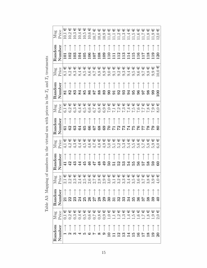
Tab

leA

3:M

appin

gof

num

ber

sin

the

vir

tual

urn

wit

hpri

ces

inth

eT2

andT3

trea

tmen

ts

Random

Num

ber

Mug

Pri

ceR

an

dom

Nu

mb

er

Mug

Pri

ceR

andom

Num

ber

Mug

Pri

ceR

andom

Num

ber

Mug

Pri

ceR

andom

Num

ber

Mug

Pri

ceR

andom

Num

ber

Mug

Pri

ce1−→

0,1e

21−→

2,1e

41−→

4,1e

61−→

6,1e

81−→

8,1e

101−→

10,1e

2−→

0,2e

22−→

2,2e

42−→

4,2e

62−→

6,2e

82−→

8,2e

102−→

10,2e

3−→

0,3e

23−→

2,3e

43−→

4,3e

63−→

6,3e

83−→

8,3e

103−→

10,3e

4−→

0,4e

24−→

2,4e

44−→

4,4e

64−→

6,4e

84−→

8,4e

104−→

10,4e

5−→

0,5e

25−→

2,5e

45−→

4,5e

65−→

6,5e

85−→

8,5e

105−→

10,5e

6−→

0,6e

26−→

2,6e

46−→

4,6e

66−→

6,6e

86−→

8,6e

106−→

10,6e

7−→

0,7e

27−→

2,7e

47−→

4,7e

67−→

6,7e

87−→

8,7e

107−→

10,7e

8−→

0,8e

28−→

2,8e

48−→

4,8e

68−→

6,8e

88−→

8,8e

108−→

10,8e

9−→

0,9e

29−→

2,9e

49−→

4,9e

69−→

6,9e

89−→

8,9e

109−→

10,9e

10−→

1,0e

30−→

3,0e

50−→

5,0e

70−→

7,0e

90−→

9,0e

110−→

11,0e

11−→

1,1e

31−→

3,1e

51−→

5,1e

71−→

7,1e

91−→

9,1e

111−→

11,1e

12−→

1,2e

32−→

3,2e

52−→

5,2e

72−→

7,2e

92−→

9,2e

112−→

11,2e

13−→

1,3e

33−→

3,3e

53−→

5,3e

73−→

7,3e

93−→

9,3e

113−→

11,3e

14−→

1,4e

34−→

3,4e

54−→

5,4e

74−→

7,4e

94−→

9,4e

114−→

11,4e

15−→

1,5e

35−→

3,5e

55−→

5,5e

75−→

7,5e

95−→

9,5e

115−→

11,5e

16−→

1,6e

36−→

3,6e

56−→

5,6e

76−→

7,6e

96−→

9,6e

116−→

11,6e

17−→

1,7e

37−→

3,7e

57−→

5,7e

77−→

7,7e

97−→

9,7e

117−→

11,7e

18−→

1,8e

38−→

3,8e

58−→

5,8e

78−→

7,8e

98−→

9,8e

118−→

11,8e

19−→

1,9e

39−→

3,9e

59−→

5,9e

79−→

7,9e

99−→

9,9e

119−→

11,9e

20−→

2,0e

40−→

4,0e

60−→

6,0e

80−→

8,0e

100−→

10,0e

120−→

12,0e

15