MPRAMunich Personal RePEc Archive

Fiscal and Monetary Policy Interactionsin Pakistan Using a Dynamic StochasticGeneral Equilibrium Framework

Muhammad Shahid and Abdul Qayyum and Waseem Shahid

Pakistan Institute of Development Economics”Quaid e Azam

University, Islamabad

July 2016

Online at https://mpra.ub.uni-muenchen.de/72595/MPRA Paper No. 72595, posted 17 July 2016 13:08 UTC

Fiscal and Monetary Policy Interactions in Pakistan Using a

Dynamic Stochastic General Equilibrium Framework

by

Muhammad Shahid* , Abdul Qayyum

† nd Waseem Shahid

**

ABSTARCT

Currently Pakistan’s economy is under stress and registered a sluggish growth for many years in

a row. The performance of major economic indicators is not satisfactory. Low investment,

double digit inflation, fiscal imbalances and low external capital inflows indicates the severity of

the grave economic situation. This paper investigates fiscal and monetary policy interaction in

Pakistan using dynamic stochastic general equilibrium model. Finding of the paper reveals that

fiscal and monetary policy interacts with each other and with other macroeconomic variables.

Inflation responds to fiscal policy shocks in the form of government spending, revenue and

borrowing shocks. Monetary authority’s decisions are also affecting fiscal policy variables. It is

also evident that fiscal discipline is critical for the effective formulation and execution of

monetary policy.

Key Words: Monetary Policy, Fiscal Dominance, DSGE, Pakistan.

JEL Classifications: E32, E37, E52, E61, E63,

* Muhammad Shahid <shahidpide@gmail.com> is a PhD student of Economics at Pakistan Institute of Development

Economics, Islamabad, Pakistan. This paper is a part of PhD Dissertation of Muhammad Shahid. †Abdul Qayyum < qayyumdr@hotmail.com> Joint Director at Pakistan Institute of Development Economics,

Islamabad, Pakistan and is the principal supervisor. ** Waseem Shahid, Assistant Professor, Quaid e Azam University, Islamabad, as Co-Supervisor The authors’ would appreciate comments/feedback on this paper. Finally, the views expressed in this paper are those of the authors and not necessarily of the Pakistan Institute of Development Economics. The other usual disclaimer also applies.

1. INTRODUCTION

Currently Pakistan’s economy is under stress and registered a sluggish growth for many

years in a row. Economy is passing through the difficult time of its history. Outlook is bleak and

gloomy. The performance of major economic indicators is not satisfactory. Low investment,

persistent and high inflation, fiscal imbalances and low external capital inflows indicates the

severity of the grave economic situation. Another important issue is the persistent and continuous

budget deficit which is the bone of contention between fiscal authority and state bank of

Pakistan. Persistence budget deficits and government borrowing deters the formulation and

execution of an independent monetary policy.

State Bank of Pakistan is adopting tight monetary policy in order to discourage

government borrowing from the domestic banking system and non-bank financial institutions,

particularly from the state bank of Pakistan. But even the higher interest rate is not working as

preventive arms to stop the federal government’s borrowing. There are many reasons, the first

and at the forefront is the friendly attitude of the State bank of Pakistan. State bank acts amicably

and never decline Federal government’s demands for fund to bridge the fiscal gap. SBP always

extends a helping hand by providing the demanded seigniorage to the government. Another issue

is the non serious attitude of the Federal government. Fiscal authority and politicians failed to

stop fiscal slippages and is not serious in ensuring fiscal consolidation and adjustments. Third,

politicians and treasury benches never allowed SBP to act and operate independently. Numerous

institutional arrangements are made and number of legislations passed from the parliament for

the independency and autonomy of State Bank of Pakistan. In 1994 monetary and fiscal policy

coordination board was formulated for greater cooperation between fiscal and monetary policy.

But significant lack of coordination has been observed over the years. From 1966 to 2012, these

authorities coordinated effectively only 13 times to achieve broad macroeconomic goals (see,

Figure 1 for self explanatory visual representation).

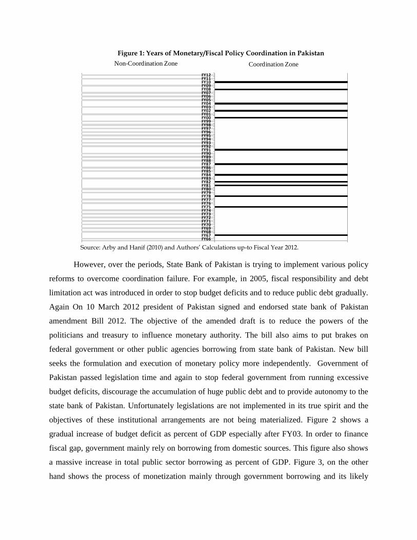
Figure 1: Years of Monetary/Fiscal Policy Coordination in Pakistan

Source: Arby and Hanif (2010) and Authors’ Calculations up-to Fiscal Year 2012.

However, over the periods, State Bank of Pakistan is trying to implement various policy

reforms to overcome coordination failure. For example, in 2005, fiscal responsibility and debt

limitation act was introduced in order to stop budget deficits and to reduce public debt gradually.

Again On 10 March 2012 president of Pakistan signed and endorsed state bank of Pakistan

amendment Bill 2012. The objective of the amended draft is to reduce the powers of the

politicians and treasury to influence monetary authority. The bill also aims to put brakes on

federal government or other public agencies borrowing from state bank of Pakistan. New bill

seeks the formulation and execution of monetary policy more independently. Government of

Pakistan passed legislation time and again to stop federal government from running excessive

budget deficits, discourage the accumulation of huge public debt and to provide autonomy to the

state bank of Pakistan. Unfortunately legislations are not implemented in its true spirit and the

objectives of these institutional arrangements are not being materialized. Figure 2 shows a

gradual increase of budget deficit as percent of GDP especially after FY03. In order to finance

fiscal gap, government mainly rely on borrowing from domestic sources. This figure also shows

a massive increase in total public sector borrowing as percent of GDP. Figure 3, on the other

hand shows the process of monetization mainly through government borrowing and its likely

-1 0 1

FY66FY67FY68FY69FY70FY71FY72FY73FY74FY75FY76FY77FY78FY79FY80FY81FY82FY83FY84FY85FY86FY87FY88FY89FY90FY91FY92FY93FY94FY95FY96FY97FY98FY99FY00FY01FY02FY03FY04FY05FY06FY07FY08FY09FY10FY11FY12

Non-Coordination Zone Coordination Zone

consequences on consumer price index (CPI) inflation. The continuous increasing trend in both

CPI inflation and borrowing behavior pushes central bank to increase its policy discount rate.

Hence, a war between fiscal and monetary authority over budget deficits and borrowing from

State Bank of Pakistan drive the debate on the interactions of fiscal and monetary policy.

Figure 2: Public Sector Borrowing, Budget Deficit and Policy Discount Rate

Figure 3: CPI Inflation, Government Borrowing and Policy Discount Rate

Therefore, we investigate in this paper the degree of interaction between fiscal and

monetary policy. Following Cebi (2012), we modify DSGE model by incorporating public sector

borrowing in the central bank reaction function. The unrestrained federal government’s

borrowing from the banking system in general and from State Bank of Pakistan in particular

forces us to include it in the model. In a recent work, Choudhari and Malik (2012) while

analyzing the objectives of monetary policy in Pakistan termed government borrowing as a

constraint on monetary policy. Monetary authority’s choice of policy instrument and the level of

7.0

9.0

11.0

13.0

15.0

17.0

19.0

21.0

0.0

2.0

4.0

6.0

8.0

10.0

12.0

14.0

16.0

18.0

20.0

FY

89

FY

90

FY

91

FY

92

FY

93

FY

94

FY

95

FY

96

FY

97

FY

98

FY

99

FY

00

FY

01

FY

02

FY

03

FY

04

FY

05

FY

06

FY

07

FY

08

FY

09

FY

10

FY

11

FY

12

Public Sector Borrowing (as % of GDP)

Budget Deficit (as percent of GDP)

Policy Discount Rate (r.h.s)

0.0

5.0

10.0

15.0

20.0

25.0

-6.0

-1.0

4.0

9.0

14.0

19.0

FY

89

FY

90

FY

91

FY

92

FY

93

FY

94

FY

95

FY

96

FY

97

FY

98

FY

99

FY

00

FY

01

FY

02

FY

03

FY

04

FY

05

FY

06

FY

07

FY

08

FY

09

FY

10

FY

11

FY

12

Government Borrowing from Banking System (as % of M2)

CPI Inflation (r.h.s)

Discount Rate (r.h.s)

inflation are greatly affected by fiscal deficits and it’s financing. This is the main reason that

forced State Bank to give weight to public finances especially Federal government borrowing

while formulating and executing monetary policy.

Economies are changing momentarily. And it is very much difficult to capture all the

dynamism, features and attributes of these changing economies. But the use of different models

enables and helps us to get closer to the real picture of the shift in economic environment.

Tracking the dynamics of fiscal and monetary policy interaction in Pakistan is important because

fiscal dominancy has important implications and state bank of Pakistan is prone to the significant

political pressure. Active fiscal policy plays a critical role in the determination of many

macroeconomic variables. Furthermore, government spending and its revenues decisions and

frequent intervention from the treasury benches undermine the effectiveness of monetary policy.

Keeping in perspective the deteriorated fiscal position of the federal government, we modified

the DSGE model with fiscal and monetary policy constraints. The objective of using DSGE

model for the interaction of fiscal and monetary policy in Pakistan is to explore avenues for the

effective formulation and execution of these policies.

The paper is designed in such a manner that section 2 describes the relevant literature

review. Section 3 illustrates dynamic stochastic general equilibrium model for the interaction of

fiscal and monetary policies. In Section 4 discuss calibration results and section 5 presents some

policy prescription in perspective of these findings and wrapping up remarks.

2. LITERATURE REVIEW

Researchers, policy makers and economic managers are increasingly interested in the use

of Dynamic Stochastic General Equilibrium Models (DSGE) for macroeconomic analysis.

Dynamic Stochastic General Equilibrium is relatively complex as compared with earlier models

for macroeconomic analysis. This paper uses small scale open economy DSGE model followed

the one used by Lubik and Schorfheide (2007), Haider and Khan (2008) and Cebi (2012). The

model is modified by incorporating fiscal authority and especially the federal government

borrowing. The main drawback of the previous models used for macroeconomic analysis like

real business cycles is the absence of room for policy intervention. Because RBC suggests that

business cycles respond to shocks optimally and there is no role of policy makers to play and

intervene through its policy instrument. On the other hand consensus exists among researcher

and academicians that DSGE model is very effective in analyzing the relationships and has the

immunity against the famous Lucas critique.

The field is new but quite enough literature is available on DSGE models due to the

increased interest of policy maker and academicians in this area. The importance of DSGE

models have forced the central bankers around the world to adopt these models for policy

making and bring it out from the contours of academic discussion. In the last several years there

is surprising developments in DSGE modeling. Following the famous Real Business Cycle

theory, Kydland and Prescott (1982) have started work on DSGE modeling. Dynamic Stochastic

general equilibrium model heavily based on the new Keynesian set up. New Keynesians school

of thought provides greater room by assigning an important role to fiscal and monetary policy for

stabilization. The inclusion of different assumptions largely contributed in the development of

DSGE model.

DSGE is frequently used by the central bankers for analyzing the effectiveness of

monetary policy while the role of fiscal policy is largely ignored. Similarly much of the attention

has been given to the monetary policy rules. The earlier version of the new Keynesians dynamic

stochastic general equilibrium models have limited role for the fiscal policy. For example, Gali

(2003) presents a symbolic and narrow role for the fiscal policy. Ratto et al., (2009) also

identified that less attention has been given to the public sector and to the interaction of fiscal

and monetary policy interaction in DSGE models. Muscatelli et al., (2004) investigate the issue

of fiscal and monetary policy interaction and modified the model by including the extended

version of fiscal policy transmission channels. They estimated the model instead of calibration.

Literature also discussed the two policies as strategic substitutes versus strategic complements.

Charles (1999) explores that fiscal and monetary policy behaves as a strategic substitutes. Hagen

et al., (2001) termed the relationship between fiscal and monetary authority as an asymmetric.

This implies that expansionary fiscal policy is accompanied by tight monetary policy stance.

Muscatelli and Mundschenk (2001) probe that the strategic substitutability of fiscal and

monetary policy does not applied to the all economies. Melitz (1997) also looked into the matter

of fiscal and monetary policy but the results are largely ambiguous. It is not clear from his

findings that the relationship between the policy instruments of the two authorities over the

period depends on policy or some structural shocks.

Strand of literatures also available on the fiscal and monetary policy interaction in a

dynamic stochastic general equilibrium model focusing a greater role for the fiscal authority.

Coenen and Straub (2005) realized the active role played by treasury in policy making and its

impact on the economy. They incorporate active and dominant fiscal policy along non-Ricardian

consumer into the DSGE model. Keeping the permanent income hypothesis, considerable

number of economic agents are non-Ricardian in nature against the standard IS curve which

heavily relied on the assumption of Ricardian equivalence. They investigate consequences of

active and dominant fiscal policy and find considerable influence of fiscal policy over

macroeconomic variables. They termed the micro-foundation and optimizing agents based model

very effective for assessing outcomes of different economic policies. Central bankers in

developed and developing economies have modified DSGE model according to the prevailing

situation in their respective economies. Tovar (2009) suggests that DSGE model is useful in

exploring the basis of instability, remarkable in the identification of structural changes, estimate

and anticipate the effects of alternate policy regime. Considerable portion of the existing

literature is contributed to the panel date but over the years, remarkable contribution by

researchers has been made to the DSGE modeling and they termed these models equally useful

for time series data. Smets and Wouters (2003) allowed for different structural shocks. They

reveal that beside panel data, DSGE models are able to calculate and predict time series data as

well. Bernanke et al (1999) also include time series data of financial fractions into DSGE

models. Cespedes et al., (2004) also investigated DSGE models while incorporating the financial

sector. They investigated the impact of firm’s balances on the investment. Choi and Cook (2004)

have incorporated banking sector and examine the performance while using DSGE model.

Milani (2004) contributed differently by comparing learning and the mechanical source of

persistence like rational expectation in habit formation or inflation indexation. Davereux and

Saito (2005) developed an alternate approach that allowed for time-varying portfolio in the

DSGE models. Engel and Matsumto (2005) kept the center of attention on complete market and

included assets markets plus portfolio choice in the DSGE model. Devereux and Sutherland

(2006) further investigated the issue and present a general formula for entire range of assets that

is compatible with DSGE models. Fabio and Sala (2006) have added to the literature by

investigating DSGE model particularly the identifiability and its repercussions for parameter

estimations. An and Schorfheide (2007) revisited the related literature with DSGE and discuss at

length the empirical implications of the model. Christiano et al., (2007) extending the model into

a small open economy framework and modified the model to include financial friction and

fraction in the labor market. Adolfson et al (2008) studied DSGE with various assumptions while

analyzing the impact of monetary policy and transmission of shocks in the economy. They also

investigate the trade-off between inflation stabilization as well as output gap stabilization with

the help of DSGE framework.

Keeping in perspective the advantages of Dynamic Stochastic General Equilibrium

models, both developed and developing economies are formulating DSGE models for their

economies. The central banks around the world are frequently using these models for analysis

and diagnosing economic problems and policy formulation. The robustness of the DSGE models

has derived the debate on the use of these models in emerging economies for policy analysis.

Following the seminal work of Christiano et al., (2005), Coenen and Straub (2005) and Cebi

(2012), model used in this thesis is an open economy DSGE model with some modification. We

modified the model by incorporating federal government borrowing from state bank of Pakistan.

We investigate the response of domestic output, taxes, inflation, monetary policy instrument and

other variables to government borrowing shock. We estimate the parameters for the economy of

Pakistan while using DSGE model in order to be consistent with the micro-foundation of our

economy.

We take two policy environments. In the first specification, we calibrate the original

DSGE model used by Cebi (2012) excluding government borrowing. In the second specification

some modification has been made while incorporate fiscal policy, particularly federal

government borrowing from state bank of Pakistan. Recognizing its significance, we check

technology as well as foreign output shocks, besides fiscal and monetary policy variables shocks.

3. MODEL SPECIFICATION

We use a small-scale open economy model for Pakistan. Following Cebi (2012), Fragetta

and Kirsanova (2010), Ortiz et al., (2009), Gali and Monacelli (2005), Fialho and Portugal

(2005), the model set in motion with infinitely lived household who seeks to maximize the

expected present discounted value of life time utility subject to inter temporal budget constraint:

11 1

0

0 1 1 1

gc n

t t t t

t c g n

C G NU E

(1)

Where 1/ 1t

is the household discount factor and 0,1 , is the inverse inters temporal

elasticity of substitution in consumption, is inverse labor supply elasticity with respect to real

wage and is relative weight on consumption of public goods. The aggregate variables in the

utility function tt GC , and tN are private consumption, government spending and labor supplied

respectively.

Household inter-temporal budget constraint:

The household inter-temporal budget constraint is

, 1 1

1t t t t t t t t t t t t

PC PG E Q D T D W N

(2)

Where , 1 1/ (1 )t t tQ r is one period ahead stochastic discount factor, tr is nominal interest rate, T

denote constant lump sum taxes and t represent income tax rate. tW is the nominal wage rate,

tD is nominal portfolio, tP is consumer price index, tC is composite consumption index which

consist of index of domestically produced goods tHC , and index of imported goods tFC , , and

tG is consumption index of public goods. These goods are produced by monopolistically

competitive firms.

1 1 1

, ,

0

H t H tC C i di

and

1 11

, ,

0

F t F tC C i di

1

, , , ,

0

. .t t H t H t F t F t

PC P i C i P i C i di

A forwarding looking open economy IS curve by solving FOC,s simultaneously is:

(3)

Where 1

And 1 1

Parameter 0 denotes elasticity of substitution between domestic and foreign goods,

measures the share of domestic consumption allocated to foreign goods (degree of openness)

, 11 1

11 1 t H tt t t t t t tc

y E y E g c r E

and reflects elasticity of substitution between the goods produced in different foreign

countries. Endogenous variables are defined as follows:

Output ln t

t t

t

Yy y y

Y

Where y denote steady state value of ty

Government spending ln 1 t

t

t

Gg

Y

Nominal interest rate tr and domestic inflation ,

,

, 1

lnH t

H t

H t

P

P

The forward looking open economy IS curve is given as:

1 1 , 1

1t t t t t t t H t

y E y E g r E

(4)

Where n

t tty y y

and n

t ttr r r

Finally n

ty

and n

tr

denote natural rate of output and nominal interest rate. These are the

equilibrium level of output and interest rate in the absence of nominal rigidities which can be

described as:

1n

t tty a c

(5)

11 1

n n n

t tt tt cr E y y c

(6)

Where ta

is the log of technology process, tA .

Behavior of the firm and price setting:

Following, Haider and Khan (2008) and Cebi (2012), there is continuum of identical

monopolistically firms in the economy. These firms produce differentiated products using linear

technology:

t t t

Y j A N j (7)

Following Calvo (1983), we assume that a fraction 1 of the firm can set a new price in each

period and a fraction of them keeps its price unchanged. To take the inflation persistency in

consideration, we also incorporate backward looking behavior in price setting process by

following Gali and Gertler (1999) and Cebi (2012):

, 1

, , 1

, 2

H tb

H t H t

H t

PP P

P

(8)

Where, 1

, 1 , 1 , 1

f b

H t h t H tP P P

is the aggregate prices chosen in period 1t by both

optimizing (forward looking, f

thP 1, ) and rule of thumb (backward looking, b

tHP 1, ) price setters.

Christiano, Eichenbaum and Evans (2005) take into account lagged dynamics in the Phillips

curve. Assuming that a fraction 1 of the firm can set a new price optimally in each period as

in calvo model, the remaining part set their prices by using the previous period inflation rate.

The rule of thumb price setter take into account the past period inflation rate , 1

, 1

, 2

H t

H t

H t

P

P

as well

as aggregate prices

1,tHP occurred in period t-1, when they reset their prices in period t. the

existence of backward looking firms besides forward looking firms allows us to obtain a log-

linearized open economy hybrid Phillips curve in terms of deviation from steady state:

, , 1 , 1b f

H t H t H tt t tE mc

(9)

n

tt t ttmc y y g

(10)

Where 1 1

b

1 1

f

1 1 1

1 1

tcm

is the marginal cost and

1ln t

t

tY

is a log-linearised tax rate. t represent cost push

shock which we include in Phillips curve by following, among others, Smet and Wouters (2007)

Beetsma and Jensen (2004), Ireland (2004), and Fragetta and Kirsanova (2010). Following Smets

and Wouters (2003) and Fragetta and Kirsanova (2010).

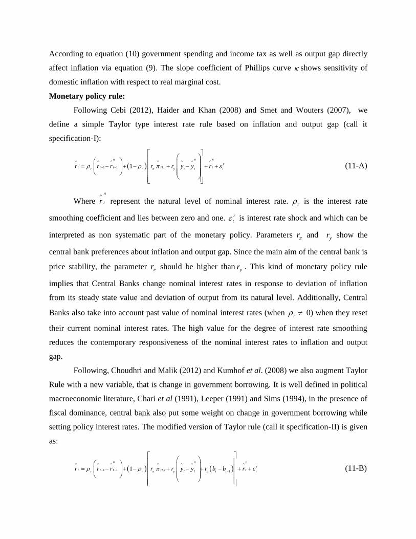
According to equation (10) government spending and income tax as well as output gap directly

affect inflation via equation (9). The slope coefficient of Phillips curve shows sensitivity of

domestic inflation with respect to real marginal cost.

Monetary policy rule:

Following Cebi (2012), Haider and Khan (2008) and Smet and Wouters (2007), we

define a simple Taylor type interest rate rule based on inflation and output gap (call it

specification-I):

1 1 ,1

n n n

rt t t tH t t tr r y t

r r r r r y y r

(11-A)

Where n

tr

represent the natural level of nominal interest rate. r is the interest rate

smoothing coefficient and lies between zero and one. r

t is interest rate shock and which can be

interpreted as non systematic part of the monetary policy. Parameters r and yr show the

central bank preferences about inflation and output gap. Since the main aim of the central bank is

price stability, the parameter r should be higher than yr . This kind of monetary policy rule

implies that Central Banks change nominal interest rates in response to deviation of inflation

from its steady state value and deviation of output from its natural level. Additionally, Central

Banks also take into account past value of nominal interest rates (when r 0) when they reset

their current nominal interest rates. The high value for the degree of interest rate smoothing

reduces the contemporary responsiveness of the nominal interest rates to inflation and output

gap.

Following, Choudhri and Malik (2012) and Kumhof et al. (2008) we also augment Taylor

Rule with a new variable, that is change in government borrowing. It is well defined in political

macroeconomic literature, Chari et al (1991), Leeper (1991) and Sims (1994), in the presence of

fiscal dominance, central bank also put some weight on change in government borrowing while

setting policy interest rates. The modified version of Taylor rule (call it specification-II) is given

as:

1 1 , 11

n n n

rt t t tH t t tr r y b t t t

r r r r r y y r b b r

(11-B)

Where, parameters r is relative weight assigned to change in government borrowing.

This specification is also consistent with an empirical paper by Malik (2007) for Pakistan

economy which also considers government borrowing as an important variable while extending

simple Taylor type monetary policy rule.

Fiscal Policy rules:

Following Cebi (2012) and Muscatelli and Tirelli (2005) we consider a backward looking

form for the fiscal policy reaction function by taking into account lagged responses of fiscal

policy to economic activity. We also assume smoothing of fiscal instruments, as Favero and

Monacelli (2005) and Forni, Monetforte and Sessa (2009).

1 1 11

n

gtt t t tg g y b t

g g g y y g b

(12)

1 1 11

n

t t t y t t b t ty y b

(13)

Parameters g and denote the degree of fiscal smoothing. Parameters yg and y demonstrate

the sensitivities of government spending and tax to past value of output gap. Parameters bg and

b correspond to feedback coefficient on unobservable debt stock. g

t and t are government

spending and tax shocks and which represent the non-systematic component of discretionary

fiscal policy.

The government solvency constraint:

Finally the model is completed by fiscal constraint. As in Cebi (2012), Kirsonva et al

(2007), and Fragetta and Kirsonva (2010) a log-linearised government solvency constraint or

fiscal constraint can be expressed as:

1 ,

11tt t H t t tt t

Cb r b y g

B

(14)

Where, , 1

ln t

t

H t

Bb

P

, tB is nominal debt stock. B is the steady state debt to GDP ratio,

and C steady state consumption to GDP ratio.

4. CALIBRATION RESULTS

In this section we estimate structural parameters values as well as shocks to the

parameters. We do determine some of the values of parameters described in the model and while

few are taken from other studies in this area particularly that of Haider and Khan (2008), Ahmad

et al., (2012), Ahmed, et al., (2012) and Choudhri and Malik (2012). Parameter’s values are

reported in Table A1. Based on these parameter values, we have calibrated model with two

monetary policy rules specifications. The statistical result in terms of variance decompositions,

cross correlations, and autocorrelations are reported in Table A2 to Table A4 and given in

Appendix section. These results fairly replicate business cycle characteristics of Pakistan

economy. Now, for policy related discussion, we would like to explain in the results of impulse

responses to exogenous shocks and want to learn how monetary and fiscal policy interacts to

each shock.

Impulse Response Analysis:

Economic theories identified and recognized numerous shocks. These shocks have

different implication for different macroeconomic variables. Some affect aggregate supply while

others affect aggregate demand. Some shock affects both aggregate demand and aggregate

supply simultaneously. There are also some sorts of shocks that affect nominal characteristics of

the economy. Figure A1 to A6 summarizes Calibration and the resulting responses of different

variable of interest to shocks.

Response of domestic Output to various shocks

In Figure A1, the first schematic presentation outlines the response of domestic output to

technology shock. The figure reveals that output follows the usual behavior and has a positive

response to technological shock. Level of domestic output deviates from the steady state as the

technology shock hits the economy. In the beginning the output increase abruptly and formed a

hum shaped. The response of domestic output also shows a high degree of persistence as it does

not returns back to its steady state up to 16 quarters. We know that DSGE model is largely based

on micro foundation and have the attributes of real business cycle. The response of domestic

output to positive technological shocks is large and considerable. This is compatible with the

existing literature as standard economic theory considers technological advancement as positive

supply shock.

Second figure shows the response of domestic output to world output shocks. It is a well

documented fact that no single country is cut off from the outside world in the current globalized

world. Higher degree of financial integration and improved means of transportation and

communication expose economies to external shocks. Mundell-Fleming model explores the

vulnerability of domestic economy to shocks, especially world output and world interest rate

shocks. These shocks are supposed to be transmitted from one economy to another. Our

economy is also vulnerable and exposed to external shock in the world economy. Keeping in

view the limitation of this thesis, we just incorporate world output shock. We employed a small

open economy DSGE model. Figure shows that domestic output responds positively to world

output shock. In the beginning domestic output rises sharply and remains above its steady state

level for 6 quarters. Then it decline for a very short period and abruptly converges to its steady

state.

The third graph shows the response of domestic output to inflation shock. High price

level damages the macroeconomic performance of the country. When inflation hits the

economy, output starts to decline and it remains below steady state for sufficiently long period of

time. The decline in output is considerable up to three quarters and then it starts rising but never

return to its steady state till 16 quarters. It implies that decline in output in response to

inflationary shock is highly persistence in Pakistan. Our calibration follows the exact

specification of Cebi. There are at least three major channels through which higher prices effect

output level in the economy. First, an increase in the price level reduces consumer’s wealth that

discourages them to spend less. A decrease in consumer’s purchasing power reduces demand in

the economy resulting a fall in the output. Second, higher price in the economy induces the

central bank to adopt tight monetary policy by increasing interest rate in the economy. Cost of

doing business goes up as the capital gets expensive with the higher interest rate. This crowded

private investment spending and reduces the overall level of output in the economy. There is

another channel through which higher prices discourages domestic output. When there is

inflationary pressure in the economy and the price level is rising, domestic currency appreciates

which in turn discourage exports. Economic activities decrease with a fall in exports causes a

decline in the domestic output. Furthermore, inflation causes the value of the currency to

decrease. People start spending their savings in the presence of inflationary pressure in the

economy. Lower saving in the country also leads to a decrease in investment and discourages

capital accumulation. The long term productivity falls that ultimately causes lower level of

domestic output. So inflation has negative impacts and hinders economic growth.

In the next schematic presentation we investigate the response of domestic output to

monetary policy. Interest rate is an important factor in the determination of output and economic

growth. In our analysis the response of domestic output to monetary policy shock is negative.

Domestic output falls with the tight monetary policy stance of the state bank of Pakistan. Output

declines and remained below steady state up to 4 quarters. After 4 quarters domestic output starts

rising but it again die out very quickly. The high responsiveness of output to monetary policy

shock implies that nominal rigidity is not hold too much in Pakistan. Because if prices are sticky

then output is not responsive too much to monetary policy shock. It means that prices are highly

flexible in Pakistan. One policy implication of the flexible prices is that policy’s role and

effectiveness declines in a more volatile price environment. Second policy implication

necessitates reforms in the behavior of interest rate. Interest rate reforms are critical because the

decision of the state bank of Pakistan regarding interest rate has critical implications for the

investment and economic activities in the country. Higher interest rate increases the cost of

doing business. Investors are unable to get cheap loans from the banking system in the presence

of higher interest rate. This harms Capital accumulation and ultimately growth in the country.

Our analysis also uncovers a decline in output in response to positive fiscal shock in the

form of higher taxes. Domestic output declines in the beginning and remain below its steady

state for a short period. Output came back to its steady state and rises for two quarters and again

die out very quickly. There are different transmission channels through which fiscal policy

shocks, tax shocks, affect output. Imposition of higher tax has legitimate economic and business

cost. Higher taxes increase price level. Higher prices and inflationary pressure in the economy

discourage productive activities and causes output to fall. Higher taxes also discourage labor

supply and employees have less incentive to work and earn more. Furthermore, tax shocks also

distort price signals and compel rational agent to substitute goods bearing lower taxes. Similarly

higher taxes discourage producers to invest and accumulate capital further. This implies that tax

shocks slow the process of economic growth and cause the domestic output to decline. The

findings are very much consistent with the standard economic literature.

We also investigate the response of domestic output to government spending shocks.

Government spends money on the purchase of goods and services. Government also incurs

expenditures on the development of infrastructures and carrying out public investments. Beside

these expenditures, government also spends money on transfer payments. Transfer payments

increases the availability of funds and purchasing power of the individuals. People spend more as

they gets more money through transfer payments. So government spending promotes economic

activity and influences growth. In the beginning domestic output expands in response to

government spending shock. Output remains above its steady state level. It comes down to its

steady state after 3 quarters and stayed there for seven quarters. Domestic output again converge

to its steady state and remained there. We know that if the government has not enough resources,

then its continuous spending undermines growth. Government extracts resources from the more

productive sectors of the economy to finance its spending on less productive activities. So in the

beginning government spending maximizes output but then it declines because expenditures are

misallocated. This implies that fiscal shock, both higher spending and higher taxes, bring

considerable volatility to domestic output. We know that volatility in the country reduces the

impact of nominal variables on real variables. The impact of financial sector of the economy,

monetary policy, has lesser impact on the real sector of the economy, fiscal policy. The impact of

policy intervention reduces considerably in the presence of volatility. Government must

rationalize its spending and its revenue behavior in order to improve the policy environment.

If we compare the two specifications, it is visible that tax shocks and government

spending shocks has a limited influence over output in the first specification. In Cebi’s

specification, he does not incorporate government borrowing from the central bank. Output

remains tied to its steady state for almost 16 quarters and fiscal shock has a negligible influence

over domestic output. This implies that federal government borrowing in Pakistan is critical

variable that affect macroeconomic variables and the overall performance.

Response of Inflation to various shocks

In Figure A2, we trace the responsiveness of inflation to different shock, particularly shock to

fiscal and monetary policy. In the first schematic presentation we report the response of inflation

to technology shock. Technology advancement has a considerable impact on output and

ultimately on inflation in the country. With a technology shock, inflation reduces because less

units of effective inputs are needed to produce the same output. Inflation reduces considerably

and remains below its steady state for very long period. It converges to its steady state almost

after 15 quarters. We have very interesting findings. If we compare the two specifications, it is

visible that when technology shock hits the economy, decline in inflation in Cebi specification is

not as much robust as in our case. This may be due to the inclusion of government borrowing

from state bank of Pakistan that is largely ignores by Cebi. Cebi’s model does not consider

government borrowing. This shows that technological shock has greater impact in the presence

of government borrowing and fiscal policy is more effective. Inflation reduces to a greater extent

in our scheme of things compare to the original model. This implies a greater role of fiscal policy

in collecting the positive spillovers of the technological shocks.

Positive world output shock causes prices in the international market to rise. The

increased economic and productivity activities leads to the rise in price of different commodity

and especially oil prices. Pakistan imports a major share of oil from the international markets.

Any increase in the world oil price has a consequential impact on the economy of Pakistan in

general and inflation in particular. The figure shows that domestic price level in the economy is

highly responsive. Inflation remains it steady state for a very long period and do not converges to

its steady state up to 16 quarters. Any rise in the world output and commodity prices cause drive

up the cost of factors of production. This has considerable impact on production and ultimately

on inflation. World output shock also causes food prices to rise

Next we document the response of inflation to monetary policy shock. Impulse response

function shows a significant decline in inflation in response to monetary policy shock. When

monetary policy shock hits the economy, inflation declines and it remains below its steady state

for sufficiently long period of time. The figure shows that inflation never returns to its steady

state up to 16 quarters. This implies that tight monetary policy stance of state bank of Pakistan is

effective in controlling inflation in the country. This also contradicts findings of the Javid and

Munir (2010). there are many possible explanations. First, data covering period as well as the

frequency of the data different. Second reason is the issue of Prize puzzle in DSGE model

discussed by Rabanal (2007). the second interesting thing between the two specification is that in

our case government has state bank of Pakistan has assigned weights to federal government from

the central bank as well as from the domestic commercial banks. Cebi model has not includes

government borrowing from the central bank and the response of inflation to tight monetary

policy shock as not significant as that in our case. In our case monetary policy is more effective

when it takes into accounts the government borrowing.

The next figure shows that a fiscal policy shocks, tax shocks, cause price level in the

economy to rise. Inflation is highly responsive to tax shock and it remains above the steady state

level. The response is also very persistent as remains there for sufficiently long time as positive

government tax shock persist, and never return to its steady state up to 16 quarters. Tax rise

increases the cost of production. Producers normally shift the incidents of taxation to the final

consumers by including taxes in the prices thus resulting upward pressure in price level in the

economy. When tax shocks hit the economy, price level rises in the economy. If we compare our

findings with Cebi’s findings, it is visible that elasticity of inflation with respect to price level in

our economy is high. This implies that in our country producers largely add taxes to the prices of

their commodity and bear less or no burden themselves.

In the next figure, we investigate response of inflation to government spending in the

country. Price level stays above its steady state for very low period and comes to its steady state

after 2 and half quarters. Then the price level start declines. One of the possible explanation for

the falling prices after 8 months is the positive impact of government spending on output. Our

results also reveals that output rises with the rise in government spending. Inflation level declines

in the economy with the increased availability of goods and services.

From this figure we observed that contractionary or tight monetary policy reduces

inflation while expansionary fiscal policy leads a price hike in the economy. This implies that

fiscal and monetary policy works in the opposite direction and the situation demands for greater

cooperation between fiscal and monetary authority in Pakistan.

Response of Interest Rate to various Shocks

In Figure A3, we investigate monetary policy response to different shocks. In the first

figure, we analyzes the response of interest rate to technology shocks. A positive technological

shock increase the interest rate in the beginning and remain above its steady state up to two

quarters. After that it immediately decline and stayed below the steady state for sufficiently long

period of time. Interest rate not come back to the steady state even up to 16 quarters. This

implies that monetary policy is expansionary in response to positive technology shock.

We also investigate the response of monetary policy to inflation shock in the economy.

State bank of Pakistan response positively by increasing the interest rate to contain the

inflationary pressure in the economy. Interest rate response actively and remain above its steady

state and not comes to its steady state up to 16 quarters. Purchasing power of money erodes with

price hike in the economy. So in order to control the erosion of purchasing power of domestic

currency and to bring price stability in the country, state bank increase its policy instrument in

response to inflation shock.

We further investigate the response of monetary policy to fiscal policy shock. We check

both tax as well as government spending shock. Interest rate rises in response to tax shocks.

Interest rate rise and it remains above its steady state for sufficiently long period of time. The

response of monetary policy is significantly persistent. These are very interesting findings. If we

compare the two specifications, it is clear that response of interest rate is not significant in Cebi’s

specification. His findings are more accurate and validate economic theory. According his

findings central bank should not increase interest rate if government obtains revenue from taxes.

Obtaining revenues from increased taxes means a contractionary fiscal policy. So it suggests an

expansionary monetary policy in order to offset the negative spillovers of the contractionary

fiscal policy. But in our case, state bank of Pakistan increases interest rate along higher tax rates.

This implies that both fiscal and monetary authority follow contractionary policies and are

making their policies independently. This should not be the case. If the fiscal branch is following

tight fiscal policy then state bank of Pakistan must adopt loose monetary policy. There is a room

for fiscal and monetary policy coordination because both higher interest rate and higher taxes

badly effect the macroeconomic performance of the country.

Here it is also very important to compare the two specifications. In Cebi’s specification,

he does not assigned any weight to government borrowing. In his set up, the response of interest

rate to technology shock is not considerable and it fell slightly. This also supports the finding of

Clarida et al., (1999) that central bank is not fully accommodative to technology and the

monetary policy is not highly responsive. The response of interest rate remains flat for

sufficiently long period of time. In our specification, we incorporate government sector and gave

weight to federal government borrowing from state bank of Pakistan. In this case interest rate

rises in the beginning, but it should not be the case. Because, according to Cebi’s specification if

government increases government taxes, then the central bank is supposed not to increase

interest rate. But in our case it is increases which is not good for the economy.

Response of Government Borrowing to various Shocks

In Figure A4, we investigate the response of government borrowing to different shocks.

The response of government borrowing to inflation in positive. When there is inflation shock in

the economy, government borrowing increases. It increases and remained above itssteadystrate

up to 7 quarters. After 7 quarters the government borrowing comes to its steadytate and stayed

there afterward till 16 quarters. The main reason is that government is now paying more and

incurred extra expenditure for the same goods and services.

Next we examine the response of government borrowing to monetary policy shocks.

Government borrowing decreases in respone of interestrate shock. Government borrowing lies

below its steady state up to 5 quarters. Then itcomes to its steady state and remained there up to

16 quarters. State bank of Pakistan knows that budget deficits and borrowing of the federal

government from state bank creating many problems. In order to contain excessive government

borrowing and the ruthless use of public exchequer. State bank of Pakistan keeps the discount

rate high in order to avoid panic and stress and to force the federal government to adopt

appropriate behavior by rationalizing its messy spending.

We also examine the response of government debt to tax shock. Government borrowing

increases in response to a positive tax shock and remain above its steady state up to 6 quarters

and then it joins its steady state level. There are many reasons for the positive response of

government borrowing to tax shock. First tax erodes production activities and discourage capital

accumulation. Low economic activities reduces government revenue from taxation and borrow

from the banking system in order to finance its expenditure. Second, tax revenue is not enough to

finance excessive federal government spending. If government expenditures are more than its

revenues, then government borrowing increases along with higher taxes in the country.

We also investigate the response of government borrowing from state bank of Pakistan to

fiscal shocks called government spending shock. Government borrowing decreases and stays

below its steady state till 16 quarters. The response shows very persistent behavior. There are

many possible justifications for the negative response of government borrowing from state bank

of Pakistan to government spending shock. For example, when the federal government increases

its spending and the expenditure are greater than the revenue generated from taxes, then

government resort state bank for providing money. State bank of Pakistan in return keeps the

discount rate higher in order to restrict government borrowing from state bank of Pakistan. In

this case it seems that monetary policy of state bank of Pakistan is effective in controlling federal

government borrowing from the state bank. Another justification is that government borrows

from external sources in order to finance its spending.

Response of Government Spending to various Shocks

In Figure A5, we trace the response of government spending to different shocks in the

economy. A rise in total factor productivity or technology shock causes domestic output to

increase. In the first figure, response of government spending to technology shock is positive.

Government spending deviates and remain above its steady state for many periods and never

returned to steady state up to 16 quarters. This implies that there is a positive relationship

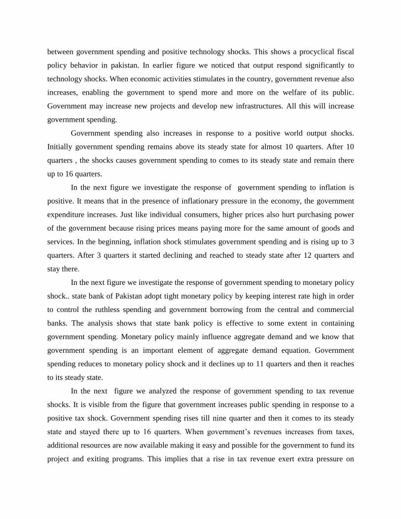
between government spending and positive technology shocks. This shows a procyclical fiscal

policy behavior in pakistan. In earlier figure we noticed that output respond significantly to

technology shocks. When economic activities stimulates in the country, government revenue also

increases, enabling the government to spend more and more on the welfare of its public.

Government may increase new projects and develop new infrastructures. All this will increase

government spending.

Government spending also increases in response to a positive world output shocks.

Initially government spending remains above its steady state for almost 10 quarters. After 10

quarters , the shocks causes government spending to comes to its steady state and remain there

up to 16 quarters.

In the next figure we investigate the response of government spending to inflation is

positive. It means that in the presence of inflationary pressure in the economy, the government

expenditure increases. Just like individual consumers, higher prices also hurt purchasing power

of the government because rising prices means paying more for the same amount of goods and

services. In the beginning, inflation shock stimulates government spending and is rising up to 3

quarters. After 3 quarters it started declining and reached to steady state after 12 quarters and

stay there.

In the next figure we investigate the response of government spending to monetary policy

shock.. state bank of Pakistan adopt tight monetary policy by keeping interest rate high in order

to control the ruthless spending and government borrowing from the central and commercial

banks. The analysis shows that state bank policy is effective to some extent in containing

government spending. Monetary policy mainly influence aggregate demand and we know that

government spending is an important element of aggregate demand equation. Government

spending reduces to monetary policy shock and it declines up to 11 quarters and then it reaches

to its steady state.

In the next figure we analyzed the response of government spending to tax revenue

shocks. It is visible from the figure that government increases public spending in response to a

positive tax shock. Government spending rises till nine quarter and then it comes to its steady

state and stayed there up to 16 quarters. When government’s revenues increases from taxes,

additional resources are now available making it easy and possible for the government to fund its

project and exiting programs. This implies that a rise in tax revenue exert extra pressure on

government to carry out additional public spending. It implies that government spending is

elastic and respond to tax revenue shocks.

Response of Government Revenue to various Shocks

Technology shocks play an important role and bring business fluctuation and economic

volatility. Our analysis shows that government revenue responds to technology shocks (Figure

A6). Total factor productivity and economic activities increase with a positive technology shock.

Income level of the economy rises. Tax revenue also increases with the rise in income in the

presence of any of the two tax system, constant or progressive tax system.

We also trace the response of tax revenue to inflation. Cost of production increase with

inflation and discourages output. Aggregate supply shrinking. In the presence of high and

volatile inflation in the economy, the producer increases the wages of the employee as the

workers often demand for increased wages. Higher price means reduction in the purchasing

power and discourage consumer spending. Agents are now paying more for goods and services.

Higher prices restrict output and reduce production. This dampen economic growth and cause

government revenue from taxes. In the start tax revenue increase with price shock. This validate

economic theory. In the beginning, price shock maximizes producer’s profit and they respond to

it by increasing production. This increase tax revenue in the short run. But this rise in the

revenue persist for a short period of two quarters and it die out very quickly. It remains below its

steady state for sufficiently large period of time and never retuned to steady state till 16 quarters.

The response of tax revenue to monetary policy shock is significant. Quantitative

tightening in the form of reduced money supply or higher interest rate increase the cost of doing

business and discourage economic activities. Higher interest rate also crowd out private

investment. In order to control the inflationary pressure in the economy, state bank of Pakistan

raises the interest rate and reduces the amount of lending. Business find it harder to get easy and

cheap credit halting economic activities to stimulate. Cost of doing business goes up. Production

activities declines and so government revenue. Higher interest rate also discourage consumers

spending. People now spend less and increases their saving. Lower economic activities reduces

government revenue from taxes. Tax revenue decreases up to 5 quarters. Tax revenue becomes to

its steady state and remained there till 16 quarters.

We also investigate the response of tax revenues to government spending shock.

Government spending increase budget deficit and interest rate. As government spending

increases, borrowing from state bank and other commercial banks also rises. This drives up

interest rate higher which increases the cost of capital. Investment crowded out and ultimately

productivity activities decline with the rising interest rate. Tax revenue also decreases with

slower economic activities. In our analysis response of tax revenue is considerable to

government spending shocks. Tax revenues deviate from steady state and not return to steady

state till 16 quarter.

5. CONCLUDING REMARKS

In this paper, we attempt to model the interaction of fiscal and monetary policy in

Pakistan in a dynamic stochastic general equilibrium model. In this scheme of things, we permit

and assign a bigger role to the fiscal policy and government borrowing. Our findings reveal that

fiscal and monetary policy interacts in Pakistan.

The key findings of our analysis reveal that fiscal and monetary policy interacts with each

others in response to shocks to different variables. We also include, government borrowing,

technology as well as foreign output shock besides fiscal and monetary policy shocks. Briefly

speaking the behavior of domestic output follows the usual behavior and has a positive response

to technological shock. Level of domestic output deviates from the steady state as the technology

shock hits the economy. Domestic output also shows a high degree of persistence. DSGE model

is largely based on micro foundation and have the attributes of real business cycle. The response

of domestic output to positive technological shocks is large and considerable and is compatible

with the existing literature as standard economic theory considers technological advancement a

positive supply shock. Our findings show that domestic output responds positively to world

output shock. Our calibration goes and investigates the response of domestic output to

inflationary shock. When inflation hits the economy, output starts to decline and it remains

below steady state for sufficiently long period of time. The decline in output is considerable up

to three quarters and then it starts rising but never return to its steady. Decline in output in

response to inflationary shock is highly persistence in Pakistan.

Interest rate is an important factor in the determination of output and economic growth.

In our analysis the response of domestic output to monetary policy shock is negative and

domestic output falls with the tight monetary policy stance of the state bank of Pakistan. The

high responsiveness of output to monetary policy shock implies that nominal rigidity is not hold

too much in Pakistan. This has very critical and important policy implications. First, role of

economic policy declines in the absence of nominal rigidity and more volatile environment.

Second policy implication necessitates reforms in the behavior of interest rate. Interest rate

reforms are critical because the decision of the state bank of Pakistan regarding interest rate has

critical implications for the investment and economic activities in the country. Our analysis also

uncovers a decline in output in response to fiscal shock in the form of higher taxes. We also

investigate the response of domestic output to government spending shocks. Domestic output

expands in response to government spending shock as increased government spending promotes

economic activities and influences growth.

In Pakistan, technology advancement has a considerable impact on output and ultimately

on inflation in the country. With a technology shock, inflation reduces because fewer units of

effective inputs are needed to produce the same output. Inflation reduces considerably in

response to technology shock. We also find that government spending responds positively and

has increased with the introduction of new technology. This implies a greater role of fiscal policy

in collecting the positive spillovers of the technological shocks. Inflation is also significantly

responsive to monetary policy shock. When monetary policy shock hits the economy, inflation

declines and it remains below its steady state for sufficiently long period of time. Tight monetary

policy stance of state bank of Pakistan is effective in controlling inflation in the country. This

contradicts findings of Javid and Munir (2010) where they find that phenomenon of price puzzle

exists in Pakistan and monetary policy is not effective. Results also show that monetary policy is

more effective when state bank gives weight to federal government borrowing. This means that

state bank of Pakistan must give weight to fiscal policy in designing its objective function while

formulating monetary policy. Inflation is also highly responsive to both the instruments of fiscal

policy shocks. Price level in the economy rises with a surge in taxes. Elasticity of inflation with

respect to taxes in Pakistan’s economy is high. This implies that producers largely add taxes to

the prices of their commodity and bear less or no burden themselves. Inflation is also responsive

and deviates from its equilibrium state with increased government spending. Contractionary or

tight monetary policy reduces inflation while expansionary fiscal policy leads a price hike in the

economy indicating that both fiscal and monetary policy works in the opposite direction and the

situation demands for greater cooperation between fiscal and monetary authority in Pakistan.

Inspecting the response of monetary policy to inflation shock in the economy unveil that

state bank of Pakistan response positively by increasing the interest rate to contain the

inflationary pressure in the economy. Examining monetary policy response to different shocks

disclose that a positive technology shock increase the policy rate. Monetary policy also respond

to fiscal policy shocks as state bank increases its policy rate to counter the negatives associated

with excessive federal government spending. Fiscal policy also responds to monetary policy

instruments. Government borrowing from state bank reduces with high policy rate. It means that

monetary policy is effective in controlling fiscal profligacy. On the other hand federal

government borrowing rises with inflation. Government borrowing also increases in response to

a positive tax shock. A rise in total factor productivity or technology shock causes government

spending to deviates and remains above its steady state indicating the pro-cyclicality of fiscal

policy in Pakistan. Government revenue rises with stimulating economic activities that enables

the government to spend more and more on the welfare of its public. Government spending to

inflation is highly elastic and increases in the presence of inflationary pressure in the economy.

Preserving price stability is critical in order to reduce the burden on already squeezed treasury.

Government expenditures are also elastic and public spending surge in response to a positive tax

shock. Tax revenue also responds negatively to inflation. Tax is very important instrument of the

fiscal policy and we report a significant response of tax to monetary policy shock. Quantitative

tightening in the form of reduced money supply or higher interest rate increase the cost of doing

business and discourage economic activities. Lower economic activities reduce government

revenue from taxes. The response of tax revenues to government spending shock is negative.

Keeping the above discussion in perspective, we come to the conclusion that fiscal and

monetary policy interacts with each other in Pakistan. So greater coordination between treasury

benches and state bank of Pakistan is needed in order to increase the effectiveness of fiscal and

monetary policy in the country.

REFERENCE

Ahmad, S., Ahmed, W., Pasha, F., Khan, S., and Rehman, M., (2012). Pakistan Economy DSGE

Model with informality. SBP Working Paper No. 47, State Bank of Pakistan.

Ahmed, W., Haider, A., and Iqbal, J., (2012). Estimation of Discount Factor and Coefficient of

Relative Risk Aversion in selected countries. SBP Working Paper No. 53, State Bank of

Pakistan.

Adolfson, M., Laséen, S., Linde, J., and Villani, M., (2008). Evaluating an estimated new

Keynesian small open economy model. Journal of Economic Dynamics and Control, 32: 2690 –

2721

Arby, M. F., and Hanif, M. N., (2010). Monetary and Fiscal Policy Coordination: Pakistan’s

Experience, SBP Research Bulletin, 6: 3 – 13.

An, S., and Schorfheide, F., (2007). Bayesian analysis of DSGE models, Econometric Reviews,

30: 889 - 920.

Beetsma, R. and Jensen, H., (2004). Mark-up Fluctations and Fiscal Policy Stabilisation in a

Monetary Union. Journal of Macroeconomics, 26(2): 357-376.

Bernanke, B., M. Gertler and S. Gilchrist (1999). The financial accelerator in a quantitative

business cycle framework, Handbook of Macroeconomics Volume, Amsterdam: Elsevier Science,

North-Holland.

Calvo, G. A., (1983). Staggered Prices in a Utility Maximizing Framework. Journal of Monetary

Economics, 12: 383 - 398.

Cebi, C., (2012). The interaction between monetary and fiscal policies in Turkey: An estimated

New Keynesian DSGE Model. Economic Modelling, 29: 1258 - 1267.

Cespedes, L, R. Chang and A. Velasco (2004). Balance sheets and exchange rate policy. The

American Economic Review, 94: 4.

Chari, V.V., L. J. Christiano and P. Kehoe (1991), Optimal monetary and fiscal policy, Some

recent results, Journal of Money, credit and banking, 23: 519- 539.

Charles, W., (1999). Economic policy coordination in EMU, Strategies and Institutions, mimeo

Choudhri, E. U., and Malik, H. A., (2012). Monetary Policy in Pakistan: A Dynamic Stochastic

General Equilibrium Analysis. IGC Working Paper 12/0389, International Growth Center (IGC),

London School of Economics and Political Science, UK.

Christiano, L., M. Eichembaum, and C. Evans, (2005). Nominal rigidities and the dynamic

effects to a shock of monetary policy, Journal of Political Economy, 113: 1 - 45.

Christiano, L., R. Motto and M Rostagno (2007). Financial factors in business cycles, Mimeo,

European Central Bank.

Choi, W. G., and D. Cook, (2004). Liability Dollarization and the Bank Balance Sheet Channel.

Journal of International Economics, 64: 247 – 282.

Clarida, R., Gali, J., and Gertler, M., (1999). The science of monetary policy: A new Keynesian

perspective, Journal of Economic Literature, 37: 1661 – 1707

Coenen, G., and Straub, R., (2005). Does government spending crowd in private consumption?

Theory and empirical evidence from the euro area. International Finance, 8(3): 435 – 470.

Devereux, M. B., and M. Saito, (2005). A Portfolio Theory of International Capital Flows.

manuscript, University of British Columbia.

Devereux, M. B., and A. Sutherland, (2006). Solving for country portfolios in an open economy

macro model. Manuscript, University of British Columbia.

Engel, C., and A. Matsumto, (2005). Portfolio choice in a monetary open-economy DSGE model.

University of Wisconsin and International Monetary Fund.

Favero, C. A., and Monacelli, T., (2005). Fiscal Policy Rules and Regime (In)Stability: Evidence

from the US. IGIER Working Paper 282.

Fabio, C., and L. Sala, (2006). Back to square one: identification issues in DSGE

models, Computing in Economics and Finance, Vol. 196.

Fialho, M. M., and Portugal, M. S., (2005). Monetary and Fiscal Policy Interactions in Brazil: An

Application of the Fiscal Theory of the Price Level. Estudos Econômicos, 35:657-685.

Forni, L., L. Monteforte, and L. Sessa (2009). The general equilibrium effects of fiscal policy:

Estimates for the Euro area. Journal of Public Economics, 93: 559 – 585.

Fragetta, M., and Kirsanova, T., (2010). Strategic Monetary and Fiscal Policy Interactions: An

Empirical Investigation, European Economic Review, 54(7): 855 – 879.

Galí, J., (2003). New Perspectives on Monetary Policy, Inflation, and the Business Cycle. In

Advances in Economic Theory, Applied Macroeconometrics, Oxford University press, 3: 151 –

197.

Galí, J. and Gertler, M., (1999). Inflation Dynamics: A Structural Econometric Analysis, Journal

of Monetary Economics, 44: 195 – 222.

Galí, J., and Monacelli, T., (2005). Monetary Policy and Exchange Rate Volatility in a Small

Open Economy, Review of Economic Studies, 72(3): 707-734.

Hagen, J. V., and Mundschenk, S., (2001). The political economy of policy coordination in the

EMU, Swedish Economic Policy Review, 8: 107 – 137.

Haider, A. and Khan, S. U. (2008a). Does Volatility in Government Borrowing Lead to Higher

Inflation? Evidence from Pakistan. Journal of Applied Economic Sciences, 4: 187 - 202.

Haider, A. and Khan, S. U., (2008b). A Small Open Economy DSGE Model for Pakistan.

Pakistan Development Review, 47(4): 963 – 1008.

Ireland, P., (2004). Technology Shocks in the New Keynesian Model. The Review of Economics

and Statistics, MIT Press, 86: 923-936.

Jacques, M. (1997). Some Cross-Country Evidence about Debt, Deficits, and the Behavior of

Monetary and Fiscal Authorities. CEPR Discussion, Paper No.1653.

Javid, M., and Munir, K., (2010). The Price Puzzle and Monetary Policy Transmission

Mechanism in Pakistan: Structural Vector Autoregressive Approach. The Pakistan Development

Review, Pakistan Institute of Development Economics, 49(4): 449 – 460.

Kirsanova, T., Satchi, M., Vines, D., and Wren-Lewis, S., (2007). Optimal fiscal policy rules in a

monetary union. Journal of Money, Credit, and Banking, 39 (7): 1759–1784.

Kydland, F. E., and Prescott, E., (1982). Time to Build and Aggregate Fluctuations.

Econometrica, 50: 1345 - 1370.

Kumhof, M and D Laxton (2007). A party without a hangover? On the effects of US government

deficits, mimeo IMF.

Kumhof, M., R. Nunes, and I. Yakadina, (2008). Simple Monetary Rules under Fiscal

Dominance. Board of Governors of the Federal Reserve System, International Finance

Discussion Papers No. 937

Leeper, E. M. (1991). Equilibria under Active and Passive Monetary and Fiscal Policies. Journal

of Monetary Economics, 27(1): 129-147.

Lubik, T. A., and Schorfheide, F., (2005). A Bayesian look at new open economy

macroeconomics. National Bureau of Economic Research 20: 313 - 366.

Lubik, T. A., and Schorfheide, F., (2007). Do central bank responds to exchange rate

movements? A structural investigation. Journal of Monetary Economics, 54: 1069 – 1087.

Malik, W. S., (2007). Monetary Policy Objectives in Pakistan: An Empirical Investigation,

Working Paper. 35, Pakistan Institute of Development Economics, Islamabad, Pakistan.

Mélitz, J., (1997). Some Cross-Country Evidence about Debt, Deficits and the Behaviour of

Monetary and Fiscal Authorities. CEPR Discussion Papers 1653, C.E.P.R. Discussion Papers.

Milani, F. (2004). Adaptive Learning and Inflation Persistence. Mimeo, Princeton University.

Muscatelli, A. M., P. Tirelli and C. Trecroci (2001). Monetary and Fiscal Policy interactions

over the Cycles: Some empirical Evidence. Cambridge University Press, Cambridge, United

Kingdom.

Muscatelli, A. M., P. Tirelli and C. Trecroci (2004). Fiscal and monetary policy interactions in a

new Keynesian Model with Liquidity constraints. Centre for Dynamic Macroeconomic Analysis,

CDMC 04/02.

Muscatelli, V.A., and Tirelli, P., (2005). Analyzing the interaction of monetary and fiscal policy:

Does fiscal policy play a valuable role in stabilisation? CESifo Economic Studies, 51 (4): 549–

585.

Ortiz, A., Ottonello, P., Sturzenegger, F. and Talvi, E. (2009). Monetary and Fiscal Policies in a

Sudden Stop: Is Tighter Brighter? In Dealing with an International Credit Crunch: Policy

Responses to Sudden Stops in Latin America, Report Draft, Inter-American Development Bank.

Rabanal, P., (2007). Does inflation increase after a monetary policy tightening? Answers based

on an estimated DSGE model, Journal of Economic Dynamics and Control, 31(3): 906 – 937.

Ratto, M., Roeger, W., and Veld, J., (2009). Fiscal policy in an estimated open- economy model

for the euro area. Economic Modeling, 26: 222 – 233.

Sim, C., (1994). A simple model for the determination of the price level and the interaction of

monetary and fiscal policy, Economic Theory, 4: 381-399.

Smets, F., and Wouters, R., (2003). An estimated stochastic dynamic general equilibrium model

of the euro area. Journal of the European Economic Association, 1: 1123 – 1175.

Smets, F., and Wouters, R., (2007). Shocks and Frictions in US Business Cycles: A Bayesian

DSGE Approach. American Economic Review, 97(3): 586 – 606.

Tovar, C. E., (2009). DSGE models and central banks. Economics - The Open-Access, Open-

Assessment E-Journal, Kiel Institute for the World Economy, 3(16):1 – 31.

RESULTS APPENDIX

TABLE A1: Selection of Parameter Values

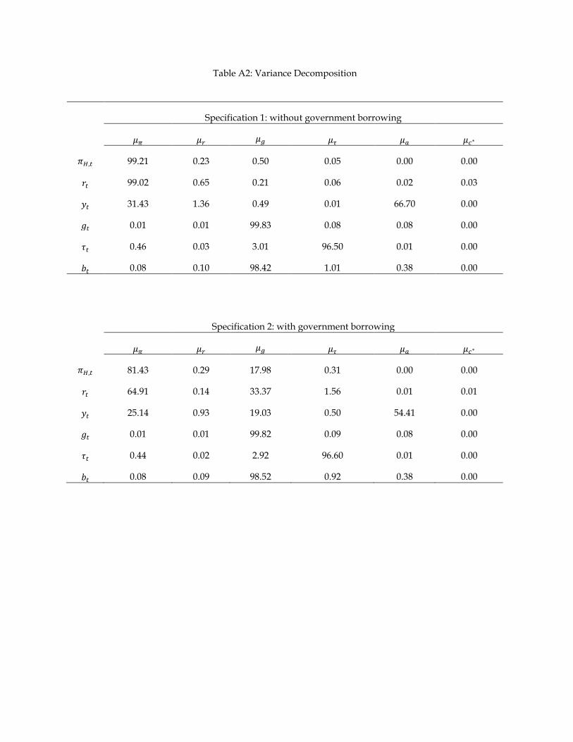
Table A2: Variance Decomposition

Specification 1: without government borrowing

99.21 0.23 0.50 0.05 0.00 0.00

99.02 0.65 0.21 0.06 0.02 0.03

31.43 1.36 0.49 0.01 66.70 0.00

0.01 0.01 99.83 0.08 0.08 0.00

0.46 0.03 3.01 96.50 0.01 0.00

0.08 0.10 98.42 1.01 0.38 0.00

Specification 2: with government borrowing

81.43 0.29 17.98 0.31 0.00 0.00

64.91 0.14 33.37 1.56 0.01 0.01

25.14 0.93 19.03 0.50 54.41 0.00

0.01 0.01 99.82 0.09 0.08 0.00

0.44 0.02 2.92 96.60 0.01 0.00

0.08 0.09 98.52 0.92 0.38 0.00

Table A3: Matrix of Correlation

Specification 1: without government borrowing

1.00 0.99 -0.55 -0.06 -0.03 0.08

0.99 1.00 -0.57 -0.03 -0.34 0.06

-0.55 -0.57 1.00 0.08 0.03 0.00

-0.06 -0.03 0.08 1.00 -0.15 -0.96

-0.03 -0.03 0.03 -0.15 1.00 0.27

0.08 0.06 0.00 -0.96 0.27 1.00

Specification 2: with government borrowing

1.00 0.86 -0.41 -0.24 0.02 0.27

0.86 1.00 -0.58 -0.46 0.15 0.51

-0.41 -0.58 1.00 0.08 0.01 -0.05

-0.24 -0.46 0.08 1.00 -0.14 -0.99

0.02 0.15 0.01 -0.14 1.00 0.25

0.27 0.51 -0.05 -0.99 0.25 1.00

Table A4: Autocorrelations

Specification 1: without government borrowing

Order 1 2 3 4 5

0.922 0.792 0.655 0.530 0.424

0.925 0.796 0.660 0.535 0.429

0.967 0.919 0.868 0.822 0.780

0.931 0.810 0.678 0.554 0.446

0.438 0.158 0.058 0.026 0.015

0.844 0.694 0.562 0.451 0.358

Specification 2: with government borrowing

Order 1 2 3 4 5

0.933 0.816 0.690 0.572 0.468

0.814 0.688 0.589 0.504 0.430

0.824 0.730 0.676 0.640 0.614

0.923 0.793 0.655 0.530 0.422

0.438 0.168 0.068 0.032 0.018

0.904 0.771 0.636 0.515 0.412

Figure A1: Response of Domestic Output

0.0480

0.0500

0.0520

0.0540

0.0560

0.0580

0.0600

0.0620

1 2 3 4 5 6 7 8 9 10 11 12 13 14 15 16

Dev

iation f

rom

Ste

ady S

tate

Technology Shock (Specification 1)

Technology Shock (Specification 2)

Quarters

-0.0005

0.0000

0.0005

0.0010

0.0015

0.0020

0.0025

1 2 3 4 5 6 7 8 9 10 11 12 13 14 15 16

Dev

iatio

n f

rom

Ste

ady

Sta

te

Foreign Output Shock (Specification 1)

Foreign Output Shock (Specification 2)

Quarters

-0.1000

-0.0500

0.0000

0.0500

0.1000

0.1500

0.2000

0.2500

0.3000

1 2 3 4 5 6 7 8 9 10 11 12 13 14 15 16

Dev

iation f

rom

Ste

ady S

tate

Government Spending Shock (Specification 1)

Government Spending Shock (Specification 2)

Quarters

-0.1600

-0.1400

-0.1200

-0.1000

-0.0800

-0.0600

-0.0400

-0.0200

0.0000

1 2 3 4 5 6 7 8 9 10 11 12 13 14 15 16

Dev

iatio

n f

rom

Ste

ady

Sta

te

Inflation Shock (Specification 1)

Inflation Shock (Specification 2)

Quarters

-0.0700

-0.0600

-0.0500

-0.0400

-0.0300

-0.0200

-0.0100

0.0000

0.0100

1 2 3 4 5 6 7 8 9 10 11 12 13 14 15 16

Dev

iation f

rom

Ste

ady S

tate

Monetary Policy Shock (Specification 1)

Monetary Policy Shock (Specification 2)

Quarters

-0.0400

-0.0300

-0.0200

-0.0100

0.0000

0.0100

0.0200

0.0300

1 2 3 4 5 6 7 8 9 10 11 12 13 14 15 16

Dev

iatio

n f

rom

Ste

ady

Sta

te

Tax Revenue Shock (Specification 1)

Tax Revenue Shock (Specification 2)

Quarters

Figure A2: Response of Domestic Inflation

-0.0006

-0.0005

-0.0004

-0.0003

-0.0002

-0.0001

0.0000

1 2 3 4 5 6 7 8 9 10 11 12 13 14 15 16

Dev

iatio

n f

rom

Ste

ady

Sta

te

Technology Shock (Specification 1)

Technology Shock (Specification 2)

Quarters

-0.0001

0.0000

0.0001

0.0001

0.0002

0.0002

0.0003

0.0003

1 2 3 4 5 6 7 8 9 10 11 12 13 14 15 16

Dev

iatio

n f

rom

Ste

ady

Sta

te

Foreign Output Shock (Specification 1)

Foreign Output Shock (Specification 2)

Quarters

-0.0600

-0.0500

-0.0400

-0.0300

-0.0200

-0.0100

0.0000

0.0100

0.0200

1 2 3 4 5 6 7 8 9 10 11 12 13 14 15 16

Dev

iati

on

fro

m S

tead

y S

tate

Government Spending Shock (Specification 1)

Government Spending Shock (Specification 2)

Quarters

0.0000

0.0200

0.0400

0.0600

0.0800

0.1000

0.1200

0.1400

0.1600

1 2 3 4 5 6 7 8 9 10 11 12 13 14 15 16

Dev

iati

on

fro

m S

tead

y S

tate

Inflation Shock (Specification 1)

Inflation Shock (Specification 2)

Quarters

-0.0090

-0.0080

-0.0070

-0.0060

-0.0050

-0.0040

-0.0030

-0.0020

-0.0010

0.0000

1 2 3 4 5 6 7 8 9 10 11 12 13 14 15 16

Dev

iati

on

fro

m S

tead

y S

tate

Monetary Policy Shock (Specification 1)

Monetary Policy Shock (Specification 2)

Quarters

0.0000

0.0010

0.0020

0.0030

0.0040

0.0050

0.0060

0.0070

0.0080

0.0090

0.0100

1 2 3 4 5 6 7 8 9 10 11 12 13 14 15 16

Dev

iati

on

fro

m S

tead

y S

tate

Tax Revenue Shock (Specification 1)

Tax Revenue Shock (Specification 2)

Quarters

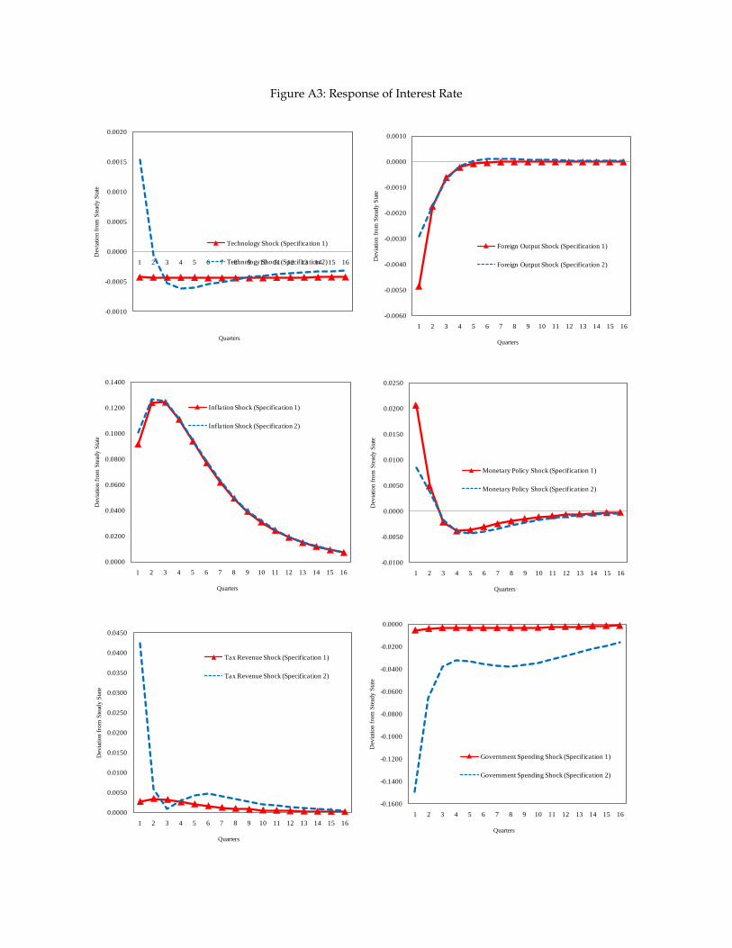
Figure A3: Response of Interest Rate

-0.0010

-0.0005

0.0000

0.0005

0.0010

0.0015

0.0020

1 2 3 4 5 6 7 8 9 10 11 12 13 14 15 16

Dev

iatio

n f

rom

Ste

ady

Sta

te

Technology Shock (Specification 1)

Technology Shock (Specification 2)

Quarters

-0.0060

-0.0050

-0.0040

-0.0030

-0.0020

-0.0010

0.0000

0.0010

1 2 3 4 5 6 7 8 9 10 11 12 13 14 15 16

Dev

iatio

n f

rom

Ste

ady

Sta

te

Foreign Output Shock (Specification 1)

Foreign Output Shock (Specification 2)

Quarters

-0.1600

-0.1400

-0.1200

-0.1000

-0.0800

-0.0600

-0.0400

-0.0200

0.0000

1 2 3 4 5 6 7 8 9 10 11 12 13 14 15 16

Dev

iation f

rom

Ste

ady S

tate

Government Spending Shock (Specification 1)

Government Spending Shock (Specification 2)

Quarters

0.0000

0.0200

0.0400

0.0600

0.0800

0.1000

0.1200

0.1400

1 2 3 4 5 6 7 8 9 10 11 12 13 14 15 16

Dev

iation f

rom

Ste

ady S

tate

Inflation Shock (Specification 1)

Inflation Shock (Specification 2)

Quarters

-0.0100

-0.0050

0.0000

0.0050

0.0100

0.0150

0.0200

0.0250

1 2 3 4 5 6 7 8 9 10 11 12 13 14 15 16

Dev

iation f

rom

Ste

ady S

tate

Monetary Policy Shock (Specification 1)

Monetary Policy Shock (Specification 2)

Quarters

0.0000

0.0050

0.0100

0.0150

0.0200

0.0250

0.0300

0.0350

0.0400

0.0450

1 2 3 4 5 6 7 8 9 10 11 12 13 14 15 16

Dev

iation f

rom

Ste

ady S

tate

Tax Revenue Shock (Specification 1)

Tax Revenue Shock (Specification 2)

Quarters

Figure A4: Response of Government Borrowing

0.0000

0.0020

0.0040

0.0060

0.0080

0.0100

0.0120

0.0140

0.0160

1 2 3 4 5 6 7 8 9 10 11 12 13 14 15 16

Dev

iation f

rom

Ste

ady S

tate

Technology Shock (Specification 1)

Technology Shock (Specification 2)

Quarters

-0.0010

0.0000

0.0010

0.0020

0.0030

0.0040

0.0050

0.0060

0.0070

0.0080

1 2 3 4 5 6 7 8 9 10 11 12 13 14 15 16

Dev

iatio

n f

rom

Ste

ady

Sta

te

Foreign Output Shock (Specification 1)

Foreign Output Shock (Specification 2)

Quarters

-0.9000

-0.8000

-0.7000

-0.6000

-0.5000

-0.4000

-0.3000

-0.2000

-0.1000

0.0000

1 2 3 4 5 6 7 8 9 10 11 12 13 14 15 16

Dev

iation f

rom

Ste

ady S

tate

Government Spending Shock (Specification 1)

Government Spending Shock (Specification 2)

Quarters

0.0000

0.0050

0.0100

0.0150

0.0200

0.0250

0.0300

0.0350

0.0400

1 2 3 4 5 6 7 8 9 10 11 12 13 14 15 16

Dev

iation f

rom

Ste

ady S

tate

Inflation Shock (Specification 1)

Inflation Shock (Specification 2)

Quarters

-0.0500

-0.0450

-0.0400

-0.0350

-0.0300

-0.0250

-0.0200

-0.0150

-0.0100

-0.0050

0.0000

0.0050

1 2 3 4 5 6 7 8 9 10 11 12 13 14 15 16

Dev

iation f

rom

Ste

ady S

tate

Monetary Policy Shock (Specification 1)

Monetary Policy Shock (Specification 2)

Quarters

-0.0200

0.0000

0.0200

0.0400

0.0600

0.0800

0.1000

0.1200

0.1400

0.1600

1 2 3 4 5 6 7 8 9 10 11 12 13 14 15 16

Dev

iatio

n f

rom

Ste

ady

Sta

te

Tax Revenue Shock (Specification 1)

Tax Revenue Shock (Specification 2)

Quarters

Figure A5: Response of Government Spending

0.0000

0.0001

0.0001

0.0002

0.0002

0.0003

0.0003

0.0004

0.0004

0.0005

1 2 3 4 5 6 7 8 9 10 11 12 13 14 15 16

Dev

iation f

rom

Ste

ady S

tate

Technology Shock (Specification 1)

Technology Shock (Specification 2)

Quarters

0.0000

0.0000

0.0000

0.0001

0.0001

0.0001

0.0001

1 2 3 4 5 6 7 8 9 10 11 12 13 14 15 16

Dev

iation f

rom

Ste

ady S

tate

Foreign Output Shock (Specification 1)

Foreign Output Shock (Specification 2)

Quarters

0.0000

0.0100

0.0200

0.0300

0.0400

0.0500

0.0600

1 2 3 4 5 6 7 8 9 10 11 12 13 14 15 16

Dev

iation f

rom

Ste

ady S

tate

Government Spending Shock (Specification 1)

Government Spending Shock (Specification 2)

Quarters

0.0000

0.0001

0.0002

0.0003

0.0004

0.0005

0.0006

0.0007

1 2 3 4 5 6 7 8 9 10 11 12 13 14 15 16

Dev

iation f

rom

Ste

ady S

tate

Inflation Shock (Specification 1)

Inflation Shock (Specification 2)

Quarters

-0.0007

-0.0006

-0.0005

-0.0004

-0.0003

-0.0002

-0.0001

0.0000

1 2 3 4 5 6 7 8 9 10 11 12 13 14 15 16

Dev

iation f

rom

Ste

ady S

tate

Monetary Policy Shock (Specification 1)

Monetary Policy Shock (Specification 2)

Quarters

0.0000

0.0005

0.0010

0.0015

0.0020

0.0025

1 2 3 4 5 6 7 8 9 10 11 12 13 14 15 16

Dev

iation f

rom

Ste

ady S

tate

Tax Revenue Shock (Specification 1)

Tax Revenue Shock (Specification 2)

Quarters

Figure A6: Response of Tax Revenue

0.0000

0.0000

0.0000

0.0000

0.0000

0.0001

0.0001

0.0001

0.0001

0.0001

0.0001

1 2 3 4 5 6 7 8 9 10 11 12 13 14 15 16

Dev

iation f

rom

Ste

ady S

tate

Technology Shock (Specification 1)

Technology Shock (Specification 2)

Quarters

0.0000

0.0000

0.0000

0.0000

0.0000

0.0000

0.0000

0.0000

0.0000

0.0000

1 2 3 4 5 6 7 8 9 10 11 12 13 14 15 16

Dev

iation f

rom

Ste

ady S

tate

Foreign Output Shock (Specification 1)

Foreign Output Shock (Specification 2)

Quarters

-0.0060

-0.0050

-0.0040

-0.0030

-0.0020

-0.0010

0.0000

1 2 3 4 5 6 7 8 9 10 11 12 13 14 15 16

Dev

iation f

rom

Ste

ady S

tate

Government Spending Shock (Specification 1)

Government Spending Shock (Specification 2)

Quarters

-0.0020

-0.0015

-0.0010

-0.0005

0.0000

0.0005

1 2 3 4 5 6 7 8 9 10 11 12 13 14 15 16

Dev

iatio

n f

rom

Ste

ady

Sta

te

Inflation Shock (Specification 1)

Inflation Shock (Specification 2)

Quarters

-0.0009

-0.0008

-0.0007

-0.0006

-0.0005

-0.0004

-0.0003

-0.0002

-0.0001

0.0000

0.0001

1 2 3 4 5 6 7 8 9 10 11 12 13 14 15 16

Dev

iation f

rom

Ste

ady S

tate

Monetary Policy Shock (Specification 1)

Monetary Policy Shock (Specification 2)

Quarters

-0.0100

0.0000

0.0100

0.0200

0.0300

0.0400

0.0500

0.0600

1 2 3 4 5 6 7 8 9 10 11 12 13 14 15 16

Dev

iatio

n f

rom

Ste

ady

Sta

te

Tax Revenue Shock (Specification 1)

Tax Revenue Shock (Specification 2)

Quarters