Embed Size (px)
Citation preview

MPRAMunich Personal RePEc Archive
Growth effects of U.S. FDI in 64developing economies, 1980 – 2007: Therole of absoptive capabilities
Krishna Chaitanya Vadlamannati
University of Santiago de Compostela
17. April 2009
Online at http://mpra.ub.uni-muenchen.de/14709/MPRA Paper No. 14709, posted 19. April 2009 04:37 UTC

1
GROWTH EFFECTS OF U.S. FDI IN 64 DEVELOPING ECONOMIES, 1980 – 2007 – THE ROLE OF ABSOPTIVE CAPABILITIES
Krishna Chaitanya Vadlamannati * [email protected]
University of Santiago de Compostela (Spain)
ABSTRACT
Both theoretical and empirical literatures have identified several channels through which FDI
influence economic growth in developing countries. This study however examines the growth
effects of U.S. FDI in 64 developing countries over the period 1980-2006. We also measure the
strength of host countries “absorptive capabilities” to adopt and adapt the foreign technology from
an advanced country like U.S. The relative differences in factor endowments between the U.S.
and individual host countries along with economic and institutional policy reforms are used as
absorptive capabilities in this study. Using aggregate production function augmented with U.S.
FDI inflows, policy reforms, factor endowment differences and their interactions with U.S. FDI
demonstrate that: (a) irrespective of capability level, an increase in the stock of U.S. FDI effects
output growth positively. (b) After controlling for omitted variable and endogenity bias using IV
method, the upward bias of growth effects of U.S. FDI came down from an excess of 7% to 4%.
(c) The results with respect to absorptive capabilities are mixed. While the beneficiary effects of
U.S. FDI are stronger in countries reforming economy and institutions, we could not find
significant results for dissimilarity in endowments leading to costlier technology transfers from
U.S. (d) Furthermore, the growth effects of U.S. FDI are positively significant in post cold war
period to pre-cold war era. Similarly, in post cold war period, the growth effects of U.S. FDI are
strongly positive and significant in Asia and Latin countries, while the same couldn’t be found for
Africa neither in 1980s nor in 1990s.
Keywords: FDI; economic growth; policy reforms; factor endowments
* The DO FILES of the empirical results can be obtained upon request at: [email protected] Acknowledgements: I would like to thank Dr. Indra de Soysa, professor, Political Science, NTNU, Norway and Dr. Bhaskara Rao, Research Fellow, NSWU, Australia, for the valuable discussion while I was working on the draft.

2
1. Introduction Over the last two decades, both theoretical and empirical literature has identified several channels
through which FDI influence economic growth in developing economies. In short-run, FDI
provides new capital, allowing additional investment in both human and physical capital, which
can be beneficial for developing countries facing severe liquidity constraints. On the other hand, in
long-run, the impact of FDI on developing economies is much higher and goes beyond solving
liquidity constraints, like investments in new or existing production plants generating employment
opportunities and resulting in transfer of hard and soft technologies to the host country.
Considering the short run implications on economic growth, FDI brings in much required capital
compensating for the lack of investable resources in the host country to finance the liquidity
constraints. This is quite evident in least developed countries like Africa where there is a sever
shortage of funds for implementing the projects under Millennium Development Program (MDGs
hereafter). Since investments is a key element in economic growth, financing part of investment
requirements of social development projects like MDGs trickle down the benefits to the poor and
help improve their socioeconomic conditions. FDI also benefits the poor in developing countries
indirectly by affecting the economic growth of the host country. Increasing economic growth is
extremely important for all the developing countries to improve its poor socio economic
conditions. Many countries in Africa, South Asia and parts of Latin region have a very high
poverty rate1. Only high economic growth with trickle down approach is the solution for the ills of
poverty and inequality in developing world. Many economists like Maddison (2001) opine that
this can be attained by a massive increase in investments which should result in sustained
economic welfare in the years to come. For that, the overall investment levels should be increased
substantially. In one his pioneer studies he shows how some of the emerging economies achieved
an economic growth rate of over 6 to 8% by significantly increasing their investment rate.
However, in majority of developing economies, given the fact that the economic growth is low,
pushing for higher levels of annual savings and domestic investments will be difficult2. This apart,
majority of the countries are already reeling under external debt and rising funds through more
debt meaning walking straight into a ‘debt trap’. Added to that, attracting foreign capital in the
form of portfolio investments is very risky because of lack of well matured domestic capital
markets and the volatility associated with such investments. Therefore, FDI as an investment
1 For example, in Africa: Mali has a poverty rate of 73%. In Bangladesh, the poverty rate is around 50%. 2 For example in Africa this is because of falling income and the burden of indebtedness (Khan, 2005).

3
financing source becomes very important which can supplement the domestic investable resources
for attaining a higher economic growth rate.
The long run implications of FDI inflows have numerous benefits. FDI help provide new capital,
allowing additional investment in both human and physical capital, which can be very beneficial
for developing and least developed countries. In the process, FDI also help creating job
opportunities, establishing international contacts, knowledge and information transfers. The most
important form of growth effects of FDI comes from transfer of new technology from abroad,
especially from advanced countries. The theory of the multinational firm proposes that
multinational corporations from advanced countries have technological advantage over local firms
that outweighs the cost of doing business in external markets (Caves, 1996; Markusen, 2002).
Thus, FDI inflows are generally seen as a means to incorporate new knowledge from abroad. The
inflow of new knowledge from advanced countries like U.S. benefit local firms through imitation
and learning (Findlay, 1978; Mansfield and Romeo, 1980; Blomström, 1986), providing
employment to the local people, increased competition in local markets, facilitation of human
capital mobility among firms (Fosfuri et al., 2001; Glass and Saggi, 2002). The newly obtained
technologies from advanced countries MNCs like the U.S. can have far reaching implications on
the host county. The transfer technology adapted by the local firms stimulates technical
efficiencies and thereby improving the productivity. This in turn can lead to increase in research
and development facilities paving way for local technical innovations in the host countries.
Innovation has widely been regarded in economic literature as one of the main drivers of
economic growth in the knowledge economy.
The Investment Development Path (IDP) theory developed in 1979 also highlights another
positive effect of FDI on host country. FDI in long run into resource based industries like labour-
intensive manufacturing, manufacturing that explore its physical resources etc result to the
introduction of some technology and creation of related industries either by foreign or domestic
firms. The entrance of foreign firms affects growth of all factors in the host country positively
eventually leading upgrading the host country’s “location” specific advantages. The increase in
location specific advantages and the potential collaborations of domestic firms with foreign firms
will provide guidance for the domestic firms to develop their own “ownership” advantages. The
development of “ownership” advantage in local firms can be gauged from the FDI outflows of the
host countries largely originating from the local firms.

4
However, Borensztein et al. (1995) argue that the growth effects of FDI differ across the countries.
Their theoretical model argues that the level of human capital determines the ability to adopt
foreign technology brought in by the advanced countries MNCs. They argue that larger
endowments of human capital are assumed to induce high economic growth for a given level of
FDI in the host country. Further, they show through their empirical models that countries need a
minimum level of threshold stock of human capital in order to make FDI contribute towards
higher economic growth. After Borensztein et al. (1995), extensive literature has been developed
emphasizing that the countries differ in terms of catching up of technology based on their
respective levels of capabilities. The study by Stern (1991) stresses on the importance of the
property rights protection in making host country attractive for FDI. This was followed by
Torstensson (1994) and Mauro (1995) who argue that ineffective bureaucracy and lack of proper
property rights protection can lead to inefficient allocation of resources. The prominent study post
Borensztein et al. (1995) is Balasubramanyam et al. (1996) who focuses on the role of trade policy
regime of the host country to attract more FDI and thereby economic growth. They argue that
export promoting countries attract more FDI and import substituting countries attract lower FDI.
Their empirical results support the argument that export promoting countries attract higher FDI
and thereby higher economic growth. Similarly, Ben-David (1996) show that countries with
greater trade liberalization will experience higher FDI supporting the assumption that liberalized
trade regime led FDI is important for economic growth. Olofsdotter (1998) highlights the ability
of host country to absorb technical knowhow depends on higher levels of bureaucratic efficiency
and property rights protection. In a recent pioneer study by Chousa et al. (2005) focuses on
institutional system dynamics to observe the institutional reforms-economic growth
interdependence in transition economies. They show that higher institutional quality (close to
average levels of OECD countries) attract higher amount of FDI and thereby economic growth in
22 transition countries. Very recently, Vadlamannati & Tamazian (2009) finds that the growth
effects of FDI in 80 developing countries are conditioned by higher economic reforms and
institutional constraints. Similarly, Vadlamannati et al. (2009) stresses the importance of economic
policy reforms in 33 African countries in order to close the technology gap and experience
economic growth.
Like the previous studies highlighted above from Borensztein et al. to Vadlamannati et al., this
paper will consider the host country absorptive capabilities receiving U.S. FDI in understanding
their role and impact on economic output growth. The approach of this paper however is more
general in nature and takes into consideration two key aspects of host country’s absorptive

5
capabilities, government institutional and economic policy reforms (capturing regulatory policies;
economic policies; institutional polices like property rights and corruption) and factor endowment
differences between U.S. and host countries.
There is a general perception which is widely recognized that countries may benefit from FDI
inflows only if the economic and institutional reforms policies are initiated. If the government
policies are rigid, marked with higher restrictions, regulations and lower incentives, high
bureaucratic procedures, rigid rules and regulations for business operations, lack of property rights
protection, restrictive labour laws, enforcement of contracts and so on and so forth would not only
hinder growth and development but would also affect productivity and human capital as allocation
of resources to other sectors becomes restrictive. Thus, the role of economic and institutional
reforms is important in promoting FDI and facilitate adoption of new technology from advanced
countries and thereby higher economic growth. Over the years, economists have argued that the
transfer of technology in domestic country is dependent upon the proximity of endowments
between the source and host country. The pioneer work of Findlay (1978) presents ‘technology
adaptation curve’ to explain how a firm’s decision to adapt foreign technology generated by the
advanced countries MNCs is based on the differences in domestic factor prices. This means that
the ‘cost of technology transfer’ from an MNC is deemed to be an increasing function of the
difference in factor endowments measured as Capital to Labour ratio between the U.S. economy
and developing countries under study.
Thus, I capture both these factors viz., institutional and economic policy reforms and factor
endowment differences between host and source country (U.S.) after controlling for other key
determinants to explain the growth effects of U.S. FDI. To this end, the study covers 64
developing countries across the regions of Africa, Latin America and Asia (including Middle East)
where U.S. has actively and substantially invested over a period of 1980 – 2006. For this purpose,
the aggregate production function is augmented with U.S. FDI inflows, policy reforms, factor
endowment differences and their interactions with U.S. FDI under pooled ordinary least squares
random effects method. I also control for plausible endogenity concern using Instrument Variable
method. The rest of the paper is organized as follows. Section 2 deals with model specification
derived from Solow (1956) growth accounting framework. Section 3 presents some important
stylized facts about U.S. investments in developing countries. While, 4 discuss empirical results,
section 5 concludes the study.

6
2. Model Specifications Let the aggregate production function at time t be:
Where, Y, K, L, denote: output; physical capital and labour respectively. Besides the factor inputs,
I also account for the “state of the economy” and “some unexplained technological efficiency
gains” of the basic production function. This is reflected in equation (1) as A(t). This also measure
of technical change in output per period. A(t) measures the proportionate change in output per
period when input level are held constant.
Dividing the above function by L and introducing logs equation (1) would become:
The estimation of this equation yields values of (α + β) and A. A is the value of technical progress
which is the rate of technological change. Sum of the partial elasticities (α + β) indicates the extent
of economies or diseconomies to scale. The returns to scale are constant, increasing or decreasing
if the value of (α + β) is equal to one, more than one or less than one respectively.
Introducing convergence into the equation yields nested augmented and textbook Solow model:
Where, the speed of convergence is given by:
Where, t is the length of the time period. A negative coefficient on the initial income (Y/Lt0) is
interpreted as the evidence for conditional convergence because holding constant other variables
in the regression, poorer countries will tend to experience higher growth. Barro (1991) and
Mankiw, Romer & Weil (1992) find strong support for conditional convergence. The standard
error for lambda (income convergence) is computed using Delta method as follows:

7
×
+
×
=
1001100
tantan
0
tLY
LYErrordardS
ofErrordardS
t
toλ
In the equation (3) how and where does “FDI” fit? As described above, A(t) reflects two components. Following Bassanini et al. (2001), I assume the
first component as δ(t) reflects the state of the economy, measured by important policy variables
like: policy reforms; trade openness; inflation and state vulnerability. The second component
include ψ(t) reflecting other unexplained sources which the model here does not explicitly capture.
This in growth theory is called as “exogenous technology progress”. Thus,
Where,
Where, PVt in equation (5) is the different policy variables measuring the state of the economy.
ψ(t) is the level of stock of technology, which in turn is dependent on the initial level of
technology, ψ (t0).
In the equation (2) there is no distinction between domestic capital stock and foreign capital. It is
assumed that FDI would be considered as an addition to existing capital stock. If this were the
case, then it would become difficult to gauge its impact on growth performance. The role of FDI
has become crucial as it provides new capital, allowing additional investments in human as well as
physical capital, which can be beneficial for developing countries which are capital scarce. Most
importantly, FDI is widely seen as a means of transferring and incorporating new knowledge from
outside the country. This becomes important more so when the FDI inflows are originating from
advanced countries like U.S. On the other hand, the developing countries are keen to attract U.S.
FDI not only because of the diffusion effects of ideas and innovations but would provide access to
the modern technologies. This is because not only the greater part of world’s R&D spending
comes from MNCs but they also possess control over advanced production techniques. Thus,

8
higher FDI inflows coming from advanced countries would lead to increase in the rate of
technological progress in host country and hence greater the rate of output growth (Wang, 1990;
Ram & Zhang 2002; Peri & Urban 2006).
The above arguments suggest that any increase in foreign capital specially from advanced
countries like U.S. would show up in A(t). Increase in foreign capital not only includes mere
quantity but also the quality of the capital stock. The economic theory has modeled the
development of capital stock in three different ways. One, Solow & Swan (1956) model of
“capital widening” which is mere accumulation of capital through increase in quantitative
production of existing capital goods. Two, “technology change” model of Aghion & Howitt
(1992) focusing on improving the quality of existing type of capital goods. Three, Romer (1990)
model of “technology change”, dealing with increasing the variety of new type of capital goods3.
All these three channels of capital stock improvements contribute economic growth through
production function. Thus, if A(t) is not growing, it is presumed that most of the economic growth
is coming from mere accumulation of foreign capital stock in general and not due to its quality.
This is in line with the current position of many developing countries that are in the stage of
capital accumulation4. It is argued that countries which open up their markets for FDI will first
experience an increase in foreign capital stock. In later stages once the capital accumulation has
been established, the major part of the FDI will then be associated with improving the quality of
existing foreign capital stock in the country. The accumulation of both total and U.S. FDI inflows
stock can easily be observed in the case of most of the developing countries especially during the
last decade. In future, this accumulated stock will be driven by the quality improvements. But
currently it can be formulated that the economic growth in developing countries is largely driven
by accumulation of capital stock.
Thus, the rate of technological change in developing countries evolves based on the available
amount of foreign technology in the host country. As highlighted above, assuming that much of
the technological innovations are made in advanced countries, FDI from advanced countries
becomes the only and most important source of technological progress in developing and least
developed countries. This can be explained as:
3 Both Aghion & Howitt (1992) and Romer (1990) models are called “capital deepening” models. The former is called “capital deepening via quality improvement” and the later is known as “capital deepening via increase in the variety of capital goods”. 4 It should be noted that though FDI inflows are flowing into many developing countries since 1970s, it was only in late 1980s and early 1990s the FDI inflows have actually started to surge. This surge can mostly be attributed to the policy reforms which most of the governments have initiated during this period.

9
−
=∆DT
DTAFTAtφ
λ
Where, λ is given exogenous parameter that denotes the rate of convergence, Δ At is the
technological changes in developing countries dependent on available amount of foreign
technology (AFT) over domestic technology (DT) and the ф is the share of foreign technology
that is actually adapted.
According to these theoretical groundings, I assume that the level of A(t) depends on the initial
stock of A(t0) : and the externalities from U.S. FDI inflows: . Thus,
Replacing equation (6) into (3) gives:
Denoting by Y; K; U.S. FDI for , respectively we get:
Gaining access to such advanced technologies provided by MNCs depends on the host countries
absorptive capabilities. Thus, higher the absorptive capabilities, greater the scope of absorbing the
technological innovations brought by the MNCs. Hence, ф (in equation above) would then be a
function of absorptive capabilities, which means 0)( >= ACfφ , where AC stands for
Absorptive Capabilities of a host country and ф is the share of foreign technology adopted by the
country. This means that the technical changes in the host country are positively related to the
share of foreign technology available and host country’s absorptive capabilities which help
adopting that foreign technology, thereby reducing the technology gap between the developing
and developed countries.

10
One of the most important channels through which FDI affects output growth performance is the
level of government policy reforms. Policy reforms are crucial because they provide incentives
and relax restrictions thereby promoting FDI. The FDI brought in by MNCs are engaged in
productivity-enhancing activities have to cope with several regulations and restrictions, acting as
disincentive and thereby inefficient allocation of resources. Policy reforms help relax these
regulations and frame market creating and enhancing policies. This allows reallocation of human
and physical capital in productive sectors and help increase productivity related to exploitation of
technology spillovers from FDI inflows (Egger, 2003 and Whyman & Baimbridge, 2006).
Second important absorptive capability variable is Factor endowment differences between the host
country and source country from which FDI originates, in this case, U.S. This reminds Findlay
(1978) “cost adaption curve” dealing with the increase in distance between the source and host
country in terms of capital – labour ratios (K/L hereafter). This means similar K/L ratios between
the host and sources countries, greater the effect of FDI. Thus, the growth effect of U.S.FDI on
developing countries depends on the absorptive capabilities of the host countries.
In such cases, the studies by Rodriguez & Rodrik (2000) and Winters (2004) have argued for a
conditional variable in measuring for such effects on economic growth. Similarly I assume that the
policy reforms and factor endowment differences are crucial in influencing U.S. FDI in
developing countries. Thus, I condition U.S. FDI inflows with Factor Endowment Differences and
Policy Reforms. Let these conditionality variables be: FED(t) and REF(t). The extended
specification based on equation (8):
)9(]......lnln)1([ln 0tttttttt YFEDFDISUREFFDISUFDISUKLY −×+×+++−++−=∆ υςψβψβαλ
Having laid foundation for the empirical analysis by introducing U.S. FDI into the aggregate
production function along with capability variables, several forms the equation (9) will be
estimated using the panel data method viz., Dynamic Two-way Random effects and Instrument
Variables method (IV method hence forth). These methods are used because of two important
reasons: (a) the possible unobservable effects can produce biased results (Baltagi, 2005). Based on
the sample of countries coming from different parts of the globe, I regard these effects as random
and apply two-way random effects estimator. This implies that the unobservable effects were part
of the disturbance and therefore independent of the observable explanatory variables. Another
reason for usage of two-way random effects over fixed effects is because the policy reforms and
11
factor endowment ratio are in some cases ‘time invariant’. Usage of fixed effects will be collinear
with time-invariant or largely time-invariant regressors (Beck, 2001). Also, it is not sure whether
the unobservable effects are fixed or otherwise, i.e. do they or do not vary by country and time?
(b) The estimates of the coefficients from random effects may likely to be biased. First, the
relationship between economic growth rate and U.S. FDI inflows can probably be bi-directional.
Our main interest is to examine the hypothesis whether U.S. FDI inflows has any positive effect
on economic output growth or not in developing countries and are driven by capabilities of
developed countries. But a growing economy can attract more FDI than a stagnant or slow
growing economy. Second, the bi-directional problem between the two may also arise from the
causal relationship between the policy reforms and output growth perworker. If policy reforms
cause good growth performance, then the reverse may also be true that good growth performance
is also good for policy reforms. A common statistical approach in dealing with causal and reverse
causal bias is to use instrumental variables. It is always a matter of supposition whether the
particular instrument variables selected would reduce biases or introduce new biases into the
models. After careful examination of these endogenity concerns, one lag structure for all the
independent variables along with lagged dependent variable are used as instruments. Following
Sprout & Weaver (1993) and Van den Berg (1996), I use Two Stage Least Squares Instrument
Variable (2-SLS henceforth) method.
The pooled time-series cross-sectional data may exhibit heteroskedasticity and serial correlation
problems. While these problems do not bias the estimated coefficients as pooled regression
analysis in itself is a more robust method for large sample consisting of cross section and time
series data. However, they often tend to cause biased standard errors for coefficients, producing
invalid statistical inferences. To deal with these problems, we estimated for all the models the
Huber-White robust standard errors clustered over countries. These estimated standard errors are
robust to both heteroskedasticity and to a general type of serial correlation within the cross-section
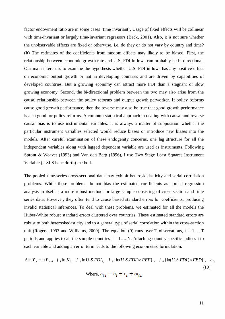
unit (Rogers, 1993 and Williams, 2000). The equation (9) runs over T observations, t = 1…..T
periods and applies to all the sample countries i = 1…..N. Attaching country specific indices i to
each variable and adding an error term leads to the following econometric formulation:
)10(})..{ln(})..{ln(..lnlnlnln ,,4,3,2,11,, tititititititi FEDFDISUREFFDISUFDISUKYY εϕϕϕϕ +×+×+++=∆ −
Where,
12
Where, Δ Yit is the dependent variable measured as change in output per working age population
(20-65) in 2000 US$ constant at PPP in country i at year t. Going by the economic growth theory,
we replace traditional measure of population with working age population because the later is
much closer to L (labour input in the production function) than the former. The data for both the
measures are from Conference Board & Groningen Growth & Development Centre, 2008.
Log Yi (t-1) is the log of real output of the working age population given in the previous year. This
variable is used mainly for the purpose of testing for convergence. This is in US$ 2000 constant in
PPP to make it comparable across the board.
Kit is the domestic investments in the host country. Many studies have used Gross Fixed Capital
Investments (GFCI henceforth) as proxy for domestic capital. However, I use ‘capital stock’
computed using Bosworth’s perpetual inventory model. Bosworth & Collins (2003) estimated
capital stock with perpetual inventory model for 84 countries that represent 95 percent of the
world’s GDP and 85 percent of the population, over a period of 40 years from 1960 to 2003. This
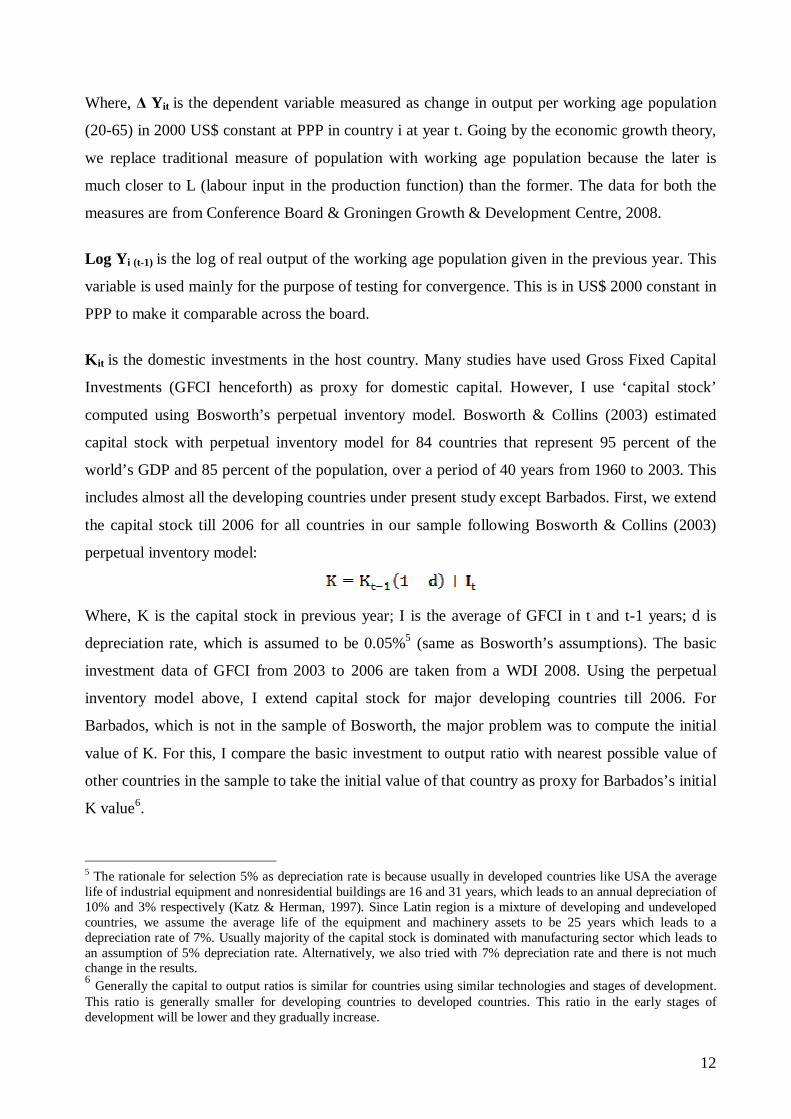
includes almost all the developing countries under present study except Barbados. First, we extend
the capital stock till 2006 for all countries in our sample following Bosworth & Collins (2003)
perpetual inventory model:
Where, K is the capital stock in previous year; I is the average of GFCI in t and t-1 years; d is
depreciation rate, which is assumed to be 0.05%5 (same as Bosworth’s assumptions). The basic
investment data of GFCI from 2003 to 2006 are taken from a WDI 2008. Using the perpetual
inventory model above, I extend capital stock for major developing countries till 2006. For
Barbados, which is not in the sample of Bosworth, the major problem was to compute the initial
value of K. For this, I compare the basic investment to output ratio with nearest possible value of
other countries in the sample to take the initial value of that country as proxy for Barbados’s initial
K value6.
5 The rationale for selection 5% as depreciation rate is because usually in developed countries like USA the average life of industrial equipment and nonresidential buildings are 16 and 31 years, which leads to an annual depreciation of 10% and 3% respectively (Katz & Herman, 1997). Since Latin region is a mixture of developing and undeveloped countries, we assume the average life of the equipment and machinery assets to be 25 years which leads to a depreciation rate of 7%. Usually majority of the capital stock is dominated with manufacturing sector which leads to an assumption of 5% depreciation rate. Alternatively, we also tried with 7% depreciation rate and there is not much change in the results. 6 Generally the capital to output ratios is similar for countries using similar technologies and stages of development. This ratio is generally smaller for developing countries to developed countries. This ratio in the early stages of development will be lower and they gradually increase.

13
U.S. FDIit is the logged U.S. FDI inflows computed using historical cost basis approach. The data
for U.S. FDI inflows is in US$ current million sourced from Bureau of Economic Analysis (BEA),
government of United States of America database on international investments. I do not consider
net U.S. FDI inflows in a host country because the U.S. capital outflows from a host country are
virtually absent for some countries. Also, it would be imperative to measure the impact of total
U.S. FDI inflows on economic growth rather than net of inflows. Using this data might encounter
some estimation problems. For some countries mostly in Africa in the initial years the U.S. FDI
inflows have registered negative values. This might be due to disinvestments or new investments
being lower than the disinvested amount. Since some of the values are in negative usage of log
becomes impossible and if the log is not used then the data will not be skewed and can generate
inconsistent results due to missing observations. To counter this problem, we make use of Busse
& Hefeker (2006) method:
Using the formula, we transform the values which bear negative signs to adopt log format. Δ REFit is change (Δ denotes: change) in economic and institutional policy reforms of the host
country. This is the first absorptive capability variable of the study. To quantify economic and
institutional policy reforms, I make use of Economic Freedom Index constructed by Gwartney,
Lawson & Easterly (2006) of Fraser institute. This index is ranked on the scale of 0 (not free) to
10 (totally free). The index captures the most objective measures of economic and institutional
reforms in a country. This index is comprehensive measure made up of five sub indices capturing:
expenditure & tax reforms; property rights & legal reforms; trade reforms; reforms related to
access to sound money; labour, business & credit reforms.
FEDit is Factor Endowment Differences between the source country (i.e. U.S.) and host country.
As discussed earlier, to create a measure of closeness between the K/L ratios of the developing
countries in the sample and U.S., I compute K/L ratios for U.S. and developing countries and
subtract the former from the later and then interact it with U.S. FDI. I follow the same measure,
but with a slight modification. Instead of taking the subtracted value, I use the following formula:

14
The square root of the subtracted value allows for an appropriate weighting on less similar host
country to U.S. FDI. Thus, the factor endowment differences variable is square root of simple
difference between K/L ratios of host countries and U.S. The interaction of this variable with U.S.
FDI captures the additional cost involved in adapting the foreign technology from advanced
countries like U.S. to domestic economy. I make use of my extension of K data of Bosworth &
Collins (2003) to compute K/L ratios for U.S. and other countries in the sample. The data for L
comes from Conference Board & Groningen Growth & Development Centre, 2008.
PVit apart from the main variables in the growth equation, I also include some of the important
policy variables which influence output growth perworker. These include: trade openness and
inflation. Higher trade openness means greater the integration and higher the competitiveness.
Finding support for trade openness affecting growth includes some of the prominent studies like:
Barro & Lee (1994); Dollar (1992); Sachs & Warner (1995); Sala-i-Martin (1997); Bassanini et al.
(2001); Barro & Sala-i-Martin (2004). Trade openness in this study is measured as: (exports +
imports)/GDP * 100. With respect to inflation, higher the value greater the macroeconomic
instability (De Melo, 1997; Bruno & Easterly, 1998). The inflation rate is measured as percentage
change in consumer price index. Data for both variables are obtained from WDI 2008.
I also include two more variables to capture macroeconomic vulnerability in developing countries.
These include: dependency on natural resources and civil war. The “resource curse” hypothesis
propounded by Sachs & Warner (1995) highlights that resource abundance impedes economic
growth. Also, natural resources, more particularly fuel and oil are characterized by the cycle of
boom and bust lead to exchange rate volatility and increase (decrease) in inflation, causing
macroeconomic uncertainty. However, the positive aspects of natural resources are that they
contribute to larger portion of exports and thereby increasing the export earnings. To capture
natural resource abundance I include the share of minerals, ores, fuel and oil exports / total
exports, data collected from WTO. Similarly, I also include civil war for macroeconomic
uncertainty (Gaibulloev & Sandler, 2008) which is a dummy coded with the value as 1 if there is a
presence of civil war in the country and 0 otherwise7.
In addition, I also include: υi representing unobservable country-specific attributes affecting
economic growth (country dummies) and εt capturing time-specific effects which vary according
to time and affects economic growth (time dummies).
7 The detailed information on data sources is given in annexure – 2.

15
3. U.S. FDI in developing countries: Some Stylized Facts In this section I present some of the important stylized facts with respect to U.S. FDI inflows,
capabilities and output growth performance of 64 developing countries. I briefly examine the host
country’s capabilities, specifically economic and institutional reforms by levels and by region and
whether they are able to reap the benefits from U.S. FDI to stimulate growth. The graph 1 presents
the U.S. FDI share in developing countries from 1966 to 2007.
Graph 1
The graph captures the share of U.S. FDI of all regions except Middle East Asia because the share
of U.S. FDI in Middle East remains fairly stable except in 1974 oil crisis period when there were
huge disinvestments. The graph 1 presents some interesting trends with respect to U.S. FDI. First,
the share of U.S. FDI in Africa has consistently declined from 1966 to 2007. Interesting
observation is that the U.S. FDI share in Africa from 1966 to 1972 was higher than that of Asia !
In 1966, U.S. FDI share in Africa was 2.6% compared to Asia’s 2.5%. This declined dramatically
post 1972 due to oil crisis. U.S. investments in Africa were largely targeted at extraction sector.
From 1977 to 1982 there was a brief increase in U.S. FDI share in Africa. But from thereon, the
U.S. FDI share in Africa declined considerably. Second, The U.S. FDI in Asia remained stagnant
till 1982. In 1982 when the oil crisis along with debt crisis struck Latin region, the U.S. MNCs
started looking at diversifying their investments from that region. Their search led them to Asia.
Hence, as one can see a dramatic rise in U.S. FDI share in Asia in 1982. The U.S. FDI inflows
started to increase from 1982 in Asia. It was about to overtake Latin region, but declined
marginally in mid and late 1990s due to South-East Asian crisis. Post 2000, the share of U.S. FDI
U.S. FDI Share across regions
0
5
10
15
20
25
1966
1968
1970
1972
1974
1976
1978
1980
1982
1984
1986
1988
1990
1992
1994
1996
1998
2000
2002
2004
2006
% s
hare
0
0.5
1
1.5
2
2.5
3
3.5
% s
hare
Latin America Asia Africa

16
in Asia overtook Latin American region. Much of this change has got to do with both the pace and
quality of economic and institutional reforms initiated by many Asian countries. This coupled with
cheap skilled labour and dramatic rise in quality of human capital helped Asia position itself as a
major investments destination for U.S. MNCs. Third, The share of U.S FDI in Latin region
declined considerably from 18.9% in 1966 to 12% in 1982 due to oil and debt crisis in the region.
From 1972 to 1984 the U.S. FDI share in Latin region almost declined every year. Post 1984, the
U.S. FDI share started to rise steadily. However, from 2000, there is a slow and steady decline in
the share of U.S. FDI in Latin region and at the same time there is a slow but steady increase in
U.S. FDI share in Asia. Proximity to U.S. and cheap labour force are the only two things which is
driving U.S. FDI into Latin America which is otherwise plagued with political instability, poor
institutional structure, civil wars and low human capital.
Graph 2
The graph 2 captures the unilateral relationship between U.S. FDI and output perworker in 64
developing countries from 1980 – 2006. The output growth performance is measured using output
growth rate per worker highlighted in section 2. For an overall 1728 observations, the output
growth rate per worker has a mean of 0.108% with a standard deviation of 5.00% (see annexure
3). This highlights that there is a significant cross-country variations. A simple correlation
between output growth rate per worker and economic reforms demonstrate a very low correlation,
r = 0.15 in the 1728 sample observations. The scatter plot in graph 2 provides a first impression of
the correlation between the output growth rate per worker and U.S. FDI inflows. Although the
data points in this plot are affected by various other factors which I will control for in the
Relationship between U.S. FDI & Output perworker growth
R2 = 0.0176-60
-50
-40
-30
-20
-10
0
10
20
30
40
50
-3 -2 -1 0 1 2 3 4 5 6
Log (U.S. FDI Inflows)
Out
put G
row
th ra
te p
erw
orke
r

17
following section in a more systematic analysis, there seems to be a positive effect of U.S. FDI on
growth. But the interesting point noteworthy is that the positive impact is only minimal and not as
high as one would have expected, especially after post 1990s which marked the end of cold war
and many developing countries initiated economic and institutional reforms.
The table 1 shows the potential links between policy reforms, U.S. FDI and output growth
performance in developing countries. In the first step, I sort all country-year-observations for
change in policy reforms into three distinct groups. These include: “high reform country-years”;
“medium reform country-years” and “low reform country-years”. This segregation was done
following a simple design viz., if the policy reforms index is in the 65th percentile of the sample,
then it is coded as “high reform country”; if the policy reforms index is under the 35th percentile of
the sample, then it is coded as “low reform country” and the countries whose reforms index fall in
between the 35th percentile and 65th percentile are coded as “medium reform countries”.
Table 1: Categorical relationship: Policy reforms, output growth perworker & U.S. FDI
Variables
Low Δ Policy Reforms
Medium Δ Policy Reforms
High Δ Policy Reforms
Δ ln (Y/L)
Total FDI U.S. FDI
Δ ln (Y/L)
Total FDI U.S. FDI
Δ ln (Y/L)
Total FDI U.S. FDI
Mean -0.32 1776.23 3174.80 0.31 1597.25 2345.61 2.51 15877.30 7760.80 Median 0.06 141.70 285.00 0.25 174.90 255.00 0.98 1081.30 4975.00
Maximum 14.82 61924.06 56851.00 20.33 69468.00 83219.00 7.03 72406.00 19016.00 Minimum -18.17 1.00 0.01 -16.50 1.00 0.01 0.17 67.11 131.00
σ 2.85 5830.28 7077.02 2.53 5328.20 7231.50 3.01 31652.54 8339.42 N 547 547 547 1173 1173 1173 5 8 8
Source: calculated & compiled by author As expected, all the three variables are stronger in high reform country-years. The mean value of
output growth rate is higher in high reform country-years followed by medium reform country-
years, while it is negative in the case of low reform country-years. The median of output growth
rate is also higher for high reform country-years. Similarly, both total FDI inflows and U.S. FDI
inflows are high in high reform country years. However, the level of volatility measured by
standard deviation for all the three indicators is associated with high reform country years.
The table 2 captures the categorization of policy reforms, U.S. FDI and output growth
performance of developing countries by regions. The regions are divided under two heads namely,
oil rich natural resources countries and non oil rich natural resources countries. The criteria

18
applied for this division is to compute the exports share of fuel and minerals from their total
exports. The countries whose fuel and minerals exports share constitute two thirds of total exports
are classified as oil rich natural resources countries.
Table 2: Categorical relationship by region
Non-Oil Resources countries
Δ ln (Y/L)
Total FDI
U.S. FDI
Reforms
Δ Reforms
Mean 0.159 1933.181 2695.593 5.674 0.061
Median 0.254 145.003 227.000 5.622 0.050 Maximum 14.819 72406.000 78436.000 9.080 0.973 Minimum -15.851 1.000 0.010 1.718 -0.975
σ 2.534 6566.571 6909.954 1.207 0.163 N 1215 1215 1215 1215 1215
Oil Resources countries
Δ ln (Y/L)
Total FDI
U.S. FDI
Reforms
Δ Reforms
Mean -0.011 1125.537 2442.063 5.378 0.063
Median 0.074 222.002 391.000 5.447 0.056 Maximum 20.331 27448.900 83219.000 7.700 1.547 Minimum -18.168 1.000 1.000 2.775 -1.125
σ 2.982 2892.132 7822.349 1.225 0.194 N 513 513 513 513 513
Source: calculated & compiled by author Some interesting findings emerge from table 2. Mean of output perworker growth rate is higher
and positive in non-oil rich countries, while the same is negative in oil rich countries. Also, the
standard deviation in the growth rate is higher in oil rich countries. Interestingly both total FDI
inflows and U.S. FDI inflows are higher in non-oil rich countries. However, the interesting point
noteworthy is that the U.S. FDI inflows are distributed in 60-40 ratio in non-oil to oil rich
countries, while this is not the case with respect to total FDI inflows. Also, the volatility of U.S.
FDI inflows in oil rich countries is higher compared to non-oil rich countries. Similar such
findings can be seen for the level of policy reforms. The current level of policy reforms is
marginally higher with low volatility in non-oil rich countries. Since the Fraser institute’s freedom
index does not change significantly every year, the gap of around 0.30 basis points between the
two regions is a reasonable lead. However, with respect to changes in policy reforms every year,
there is not much significant difference between the two regions (see mean values). Having said
that, the volatility (standard deviation) is fairly high in oil rich countries in comparison with non-
oil rich countries.

19
4. Empirical Results & Discussion The sample of country-years that we examine in total is 1728 observations. The results of
regression estimates using random effects method in assessing the growth effects of U.S. FDI are
presented in 10 different models in table 3. I also control for heteroskedasticity using Huber-White
heteroskedasticity-consistent standard errors & covariance. The summary of data is provided in
annexure 3. The model 1 in table 3 shows that the lagged value of output per worker is negative
but insignificant. The results highlight the presence of “conditional convergence”. Model 1
presents the estimated results of trivial regression where output per worker growth is exclusively
explained by U.S. FDI inflows, domestic capital stock and conditional convergence (see second
column of table 3). The U.S. FDI inflows are significant and the sign is consistent with the
theoretical predictions. The coefficient value is small and shows that for every 1% increase in
U.S. FDI lead to around 0.070% increase in output per worker growth in long run. The
convergence variable still holds to its negative sign but remains statistically insignificant. The
capital stock variable in the same model is positive and significant. We use this model as a
benchmark throughout the study. In model 2 (see table 3), the same results are ran using 2-SLS IV
method. The results show that the long run coefficient on FDI is still positive and significant. For
every 1% increase in FDI, leads to 0.051% increase in output growth performance. In other words,
holding at its mean value, increase in log FDI inflows by its highest value (log 10.4) would
increase the economic growth rate in developing countries by 0.051%. However, it is noteworthy
that both significance level and the value of coefficient for U.S. FDI inflows have come down
significantly in 2SLS IV method compared to earlier results in random effects model. This
highlights potential endogenity between the U.S. FDI inflows and output growth per worker.
Surprisingly we also find that capital stock though positive and significant has come down by
0.01% compared to the results in model 1. But, the capital stock remains statistically significant at
10% through out all the models. Another interesting finding is that the result of capital stock
without U.S. FDI inflows is insignificant8. This surprising result could be because of the
“crowding in effect” of U.S. FDI. The correlation between the two models is only 0.45%. This
explains that there is some degree of crowding in effect between U.S. FDI and domestic capital
stock in developing countries. Another interpretation can be that the available level of foreign
technology from an advanced country like the U.S. is positively affecting the existing level of
domestic technology. Furthermore, comparing the coefficients of U.S. FDI inflows and domestic
capital stock reveals that the coefficient value of the former is much higher than the later. One
8 Results not shown here due to brevity, but are provided upon request from author.

20
reason for this could be because of the rate of growth of U.S. FDI in developing countries is
exuberant compared the growth rate of domestic capital stock. Another reason could be due to
spillovers generated from transfer of technology by U.S. MNCs.
In model 3 of table 3, we include our second main variables, economic and institutional reforms
index along with factor endowment differences. We find that economic and institutional policy
reforms are positive and have significant impact on output growth performance of developing
countries. For every 1% increase in the reforms index lead to 2.16% increase in growth of output
per worker. On the other hand, we could not find any statistical significance for factor endowment
differences variable. In the same model, though the positive sign and significance level of U.S.
FDI still holds, the coefficient value has declined marginally. The coefficient value of U.S. FDI
inflows declined from 0.070% in model 1 to 0.069% in model 3. This also means that the output
growth in developing world is not only explained by U.S. FDI inflows, but there are also other
significant factors that contribute to output growth. Most important amongst them include changes
in economic and institutional policy reforms. The comparison of coefficients between FDI inflows
and policy reforms show some interesting trends. While both have positive effect on output
growth performance, the impact of policy reforms is substantially higher to U.S. FDI. The 2SLS
results in model 4 shows that the growth effects of U.S. FDI inflows is 0.051%, an upward bias of
0.020% compared to model 3. Surprisingly, the coefficient values of both policy reforms and
factor endowment differences increased marginally in model 4 to model 3. This means that the
country and period effects are more important for these two variables and correcting for
endogenity accounts for a minority of the bias.
In model 5, other control variables are introduced into the model. We find that amongst all
variables, the effect of U.S. FDI on output growth perworker is the highest after policy reforms.
The upward bias effect of U.S. FDI is corrected using IV method (see model 6, table 3). The
growth effects of U.S. FDI after correcting for endogenity come down from 0.073% to 0.040%.
With respect to other control variables, we could not find any strong significant evidence of
‘resource curse’ hypothesis. The impact of trade openness on economic growth is positively
significant only after controlling for endogenity bias9. Both the growth destabilizing variables
(inflation rate and presence of civil war) have significant negative impact on output growth
performance in developing countries during the period 1980 – 2006.
9 It is important to note that a rigid trade regime may also encourage FDI inflows because of the cost associated with trade. Usually this is labeled as “tariff jumping FDI”. For more, see Jun & Singh (1996).

21
Table 3: U.S. FDI & Host country economic growth equation function
Dependent Variable: Growth rate of Output per worker
Variables
Model 1 Model 2 Model 3 Model 4 Model 5 Model 6 Model 7 Model 8 Model 9 Model 10 POLS
Random 2-SLS-IV Random
POLS Random
2-SLS-IV Random
POLS Random
2-SLS-IV Random
POLS Random
2-SLS-IV Random
POLS Random
POLS Random
Constant
-0.515 (0.60)
-0.378 (0.53)
-0.966 (0.84)
-1.117 (0.72)
-0.912 (0.91)
-1.572 * (0.80)
0.188 (0.95)
-1.290 (0.83)
-0.958 (0.92)
-0.494 (1.18)
Lagged Dependent Variable ____ 0.299 *
(0.04) ____ 0.283 *
(0.04) ____ 0.275 *
(0.04) ____ 0.273 *
(0.04) ____ ____
Ln { Output per worker (t – 1) } -0.009 (0.08)
-0.019 (0.06)
-0.009 (0.08)
-0.006 (0.07)
-0.056 (0.08)
-0.016 (0.07)
-0.056 (0.08)
-0.014 (0.07)
-0.001 (0.08)
-0.006 (0.08)
Ln (Domestic capital Stock) 0.023 ***
(0.00) 0.022 ***
(0.01) 0.026 ***
(0.01) 0.028 ** (0.01)
0.029 *** (0.01)
0.028 ** (0.01)
0.007 (0.00)
0.022 *** (0.01)
0.032 ** (0.01)
0.032 *** (0.01)
Ln (U.S. FDI inflows) 0.070 ** (0.03)
0.051 *** (0.03)
0.069 ** (0.03)
0.051 *** (0.03)
0.073 ** (0.03)
0.040 *** (0.02)
-0.027 (0.04)
-0.069 (0.05)
0.042 (0.03)
-0.004 (0.15)
Δ Economic & Institutional Reforms ____ ____ 2.160 *
(0.48) 3.949 * (1.04)
2.160 * (0.47)
3.887 * (1.06)
2.093 * (0.46)
3.931 * (1.06)
-0.920 (0.80)
2.155 * (0.47)
Factor Endowment Differences ____ ____ 0.644
(1.19) 1.011 (1.03)
0.485 (1.35)
0.354 (1.20)
-0.219 (1.35)
0.438 (1.21)
0.588 (1.35)
0.253 (0.48)
Ln (Trade openness) ____ ____ ____ ____ 0.039
(0.13) 0.207 ***
(0.12) -0.008 (0.13)
0.193 *** (0.12)
0.061 (0.13)
0.040 (0.13)
Inflation rate ____ ____ ____ ____ -0.001 **
(0.00) -0.0003 ***
(0.00) -0.001 **
(0.00) -0.0003 ***
(0.00) -0.001 **
(0.00) -0.001 **
(0.00)
Minerals-Fuels export share ____ ____ ____ ____ -0.002
(0.00) -0.001 (0.00)
-0.002 (0.00)
-0.001 (0.00)
-0.002 (0.00)
-0.002 (0.00)
Civil War presence ____ ____ ____ ____ -0.293 ***
(0.17) -0.072 (0.19)
-0.274 *** (0.17)
-0.064 (0.19)
-0.297 *** (0.17)
-0.298 *** (0.17)

22
Ln (U.S. FDI Inflows Squared) ____ ____ ____ ____ ____ ____ 0.019 *
(0.00) 0.011 ** (0.00)
____ ____
Ln (U.S. FDI Inflows) X Δ Reforms ____ ____ ____ ____ ____ ____ ____ ____ 0.539 *
(0.16) ____
Ln (U.S. FDI Inflows) X Factor Endowment Differences
____ ____ ____ ____ ____ ____ ____ ____ ____ -1.063 (3.21)
λ – Income Convergence 0.008 *
(0.0008) 0.016 *
(0.0006) 0.008 *
(0.0008) 0.005 *
(0.0007) 0.050 *
(0.0008) 0.014 *
(0.0007) 0.050 *
(0.0008) 0.012 *
(0.0007) 0.001
(0.0008) 0.005 *
(0.0008)
R-squared 0.004631 0.098750 0.024393 0.110072 0.033797 0.107413 0.043043 0.107138 0.040918 0.033658 Adjusted R-squared 0.002899 0.096577 0.021560 0.106849 0.028735 0.102013 0.037470 0.101193 0.035332 0.028030 F-statistic 2.674 ** --------- 8.610 * --------- 6.677 * --------- 7.722 * --------- 7.325 * 5.980 * Durbin-Watson statistic 1.372111 1.943260 1.395479 1.953128 1.422925 1.958741 1.431874 1.958008 1.434088 1.424641 Number of Countries 64 64 64 64 64 64 64 64 64 64 Total Number of Observations 1728 1664 1728 1664 1728 1664 1728 1664 1728 1728 Country Dummies YES YES YES YES YES YES YES YES YES YES Period Dummies YES YES YES YES YES YES YES YES YES YES
Note: * Significant at 1% confidence level; ** Significant at 5% confidence level; *** Significant at 10% confidence level. White Heteroskedasticity-Consistent Standard Errors are reported in parenthesis. Standard error for lambda (income convergence) is computed using Delta method.

23
In model 7 and 8, we find significant curvi-linear relationship between U.S. FDI and
economic growth in developing countries. The relationship is non-linear which means the
U.S. FDI has a positive impact on output growth if they exceed a certain threshold. A
quality of FDI path exists if there is a statistically significant relationship. A path displays
a turning point if the coefficient value of U.S. FDI is < 0 and the coefficient value of
reforms squared indicator is > 0. The U.S. FDI at turning point, denoted by U.S. FDI+,
where U.S. FDI+ = (- U.S. FDI / 2 * U.S. FDI squared). The result from using this
formula is found to be 3.14. This suggests that in order to start making a significant
impact on economic growth rate, countries should have a minimum of 3.14 US$ millions
of U.S. FDI in the host country.
In last two models, I interact U.S. FDI with both absorptive capabilities variables to
measure the conditional effects of U.S. FDI on output growth perworker. The interaction
effect variable is found to be positive and significant at 1% confidence level (see model
9; table 3). This suggests that both U.S. FDI and policy reforms are compliments. The
joint effect of U.S. FDI and policy reforms on output growth is 0.54%. Thus, institutional
and economic reforms are important for the host country in order to reap the potential
benefits from U.S. FDI. However, we could not find any statistical significance for the
other interactive variable viz., U.S. FDI and factor endowment differences. The joint
effect of this capability variable has right sign but is insignificant (see model 10, table 3).
Next, I examine how the effects of U.S. FDI vary over the time and over the regions.
Specifically I allow U.S. FDI variable to have different effects over the periods of 1980 –
1990 (1980s) and 1991 – 2006 (1990s). For this purpose I create dummy variables for
each time period and interact it with log U.S. FDI inflows. Similarly, I also create dummy
variables capturing the countries falling under three regions viz., Asia; Latin America and
Africa. Models 11 - 13 in table 4 present the estimation results. First, in model 11 I
capture the interaction of U.S. FDI with period dummies. Some interesting findings
emerge from these results. First, U.S. FDI inflows are positive and significant only post-
1990s, while they are negative in the 1980s. Second, the coefficient values of U.S. FDI
inflows are higher in 1990s than 1980s. This is because the rate of growth in U.S. FDI
inflows in 1990s compared to 1980s was higher in all the developing countries. The
entire 1980s period was marked with cold war leading to U.S. shying away from

24
investing in certain countries, especially in Asian region. All this changed in the 1990s
allowing U.S. investments spread across the world.
Table 4: U.S. FDI & Host country economic growth
Dependent Variable: Growth rate of Output per worker
Variables
Model 11 Model 12 Model 13 POLS: Random POLS: Random POLS: Random
Constant
0.026 (0.87)
-1.156 (1.01)
-0.047 (1.00)
Ln {Output per worker} (t – 1) -0.008 (0.08)
-0.014 (0.09)
-0.005 (0.09)
Ln (Domestic capital) 0.018 (0.01)
0.034 ** (0.01)
0.020 (0.01)
Δ Economic & Institutional Reforms 2.075 * (0.47)
2.170 * (0.48)
1.912 * (0.47)
Factor Endowment Differences -0.844 (1.32)
0.767 (1.37)
-0.790 (1.39)
Ln (Trade openness) -0.036 (0.14)
0.075 (0.13)
-0.047 (0.14)
Inflation rate -0.001 **
(0.00) -0.001 **
(0.00) -0.0005 **
(0.00)
Minerals-Fuels export share -0.002 (0.00)
-0.002 (0.00)
-0.002 (0.00)
Civil War presence -0.300 ***
(0.17) -0.270 (0.19)
-0.255 (0.18)
Ln (U.S. FDI Inflows X 1980s -0.028 (0.04)
____ ____
Ln (U.S. FDI Inflows) X 1990s 0.107 * (0.03)
____ ____
Ln (U.S. FDI inflows) X Asia Dummy ____ 0.063 **
(0.03) ____
Ln (U.S. FDI inflows) X Latin America Dummy ____ 0.085 **
(0.04) ____
Ln (U.S. FDI inflows) X Africa Dummy
____ 0.053 *** (0.03)
____
Ln (U.S. FDI inflows) X Asia Dummy X 1980s ____ ____ 0.064 ***
(0.03)
Ln (U.S. FDI inflows) X Latin Dummy X 1980s ____ ____ -0.143 **
(0.07)
Ln (U.S. FDI inflows) X Africa Dummy X 1980s ____ ____ 0.032
(0.03)
Ln (U.S. FDI inflows) X Asia Dummy X 1990s ____ ____ 0.055 ***
(0.03)
Ln (U.S. FDI inflows) X Latin Dummy X 1990s ____ ____ 0.159 *
(0.04)
Ln (U.S. FDI inflows) X Africa Dummy X 1990s ____
____
0.035 (0.03)
λ – Income Convergence 0.007 *
(0.0008) 0.012 *
(0.0009) 0.004 ** (0.0009)

25
R-squared 0.044455 0.035077 0.073982 Adjusted R-squared 0.038889 0.028891 0.066413 F-statistic 7.987 * 5.670 * 9.775 * Durbin-Watson statistic 1.494106 1.495003 1.498591 Number of Countries 64 64 64 Total Number of Observations 1728 1728 1728 Country Dummies YES YES YES Time Dummies YES YES YES
Note: * Significant at 1% confidence level; ** Significant at 5% confidence level; *** Significant at 10% confidence level. White Heteroskedasticity-Consistent Standard Errors are reported in parenthesis.
Second, in model 12, I capture the interaction of U.S. FDI with regional dummies. The
results show that the U.S. FDI inflows have significant positive effects on all the regions.
Comparing the coefficients shows that the growth effect of U.S. FDI was highest in Latin
countries followed by Asia and Africa. The Latin American effect is probably because of
cheap labour costs and close distance to U.S. The U.S. FDI growth in Asia was largely in
post 1990s. Higher and faster economic and institutional reforms coupled with increase in
human capital and cheap skilled labour are the driving factors of U.S. FDI. However, in
the case of Africa, the U.S. FDI increased in 1989 from US$ 5 billions to US$ 36 billions
by 1997. But U.S. FDI is concentrated largely in extractive sectors in Africa and majority
of the U.S. FDI is parked in only few countries like Nigeria and South Africa which have
exogenous factors like natural resources. Clubbing the analysis for model 11 and model
12, we get the results shown in model 13. The growth effects of U.S. FDI are positive in
all the three regions only in 1990s. In the 1980s, the growth effects of U.S. FDI in Latin
countries were strongly negative because of debt and oil crisis across the region.
However, in Africa, both in 1980s and 1990s, the U.S. FDI was positive but remained
grossly insignificant.
Table 5: Output growth gains from U.S. FDI in developing countries
Variables
(full period) 1980 - 2006
(1980s) 1980 - 1990
(1990s) 1991 - 2006
U.S. FDI inflows 0.073 **
(0.03) -0.028 (0.04)
0.079 ** (0.03)
U.S. FDI inflows X Asia Dummy 0.063 **
(0.03) 0.064 ***
(0.03) 0.119 **
(0.03)
U.S. FDI inflows X Latin Dummy 0.085 **
(0.04) -0.143**
(0.07) 0.016 (0.40)
U.S. FDI inflows X Africa Dummy 0.053 ***
(0.03) 0.032 (0.03)
0.067 ** (0.03)
Source: computed & compiled by author

26
The table 5 gives a brief summary of the temporal pattern of the effects of U.S. FDI on
economic growth rate in developing countries10. The results in the first row indicate that
U.S. FDI has become increasingly important, especially in the post 1990s period. Though
similar such argument can be made for the regional interactive variables, the partial
effects coefficient jump from 1980s to 1990s is relatively higher in the case of Asia than
Latin America and Africa. However, only Asia and Latin American partial effects are
significant and not Africa. This also highlights that U.S. FDI was the most rewarding in
Asia compared to Latin America and Africa.
Table 6: Output growth gains from U.S. FDI in developing countries by region
Variables
1980 - 2006
Asian region 0.136 * (0.03)
Latin American region 0.158 * (0.03)
African region 0.126 * (0.03)
Total Sample 0.073 **
(0.03) Source: computed & compiled by author
The table 6 gives a brief summary of the temporal pattern of the effects of U.S. FDI on
output per worker by regions of Asia, Latin America and Africa11. The partial effects of
U.S. FDI inflows indicate that it has become increasingly important for all the three
regions. However, the effects are higher in Asia and Latin region compared to Africa.
One credible recommendation which can be derived from these partial effects results is
that U.S. FDI has played a very important role in affecting economic growth positively.
However, the same is not true in the case of Africa suggesting that there is a little
evidence to show that there is genuine technology transfer. As on 2002, more than 50%
of U.S. FDI inflows in Africa are concentrated in only two countries: Nigeria and South
Africa. Most importantly, the U.S. FDI in Africa largely goes into extractive industries,
thus parking the much needed investments in enclave economy. Hence, in the first place
10 The partial effects for different time periods are calculated as follows: The coefficient values of the 1980s are added to the coefficient of the basic model. Likewise, the coefficient values of the 1990s are added to the new values obtained previously for the 1980s. 11 Partial coefficients are calculated as follows: The estimated coefficients for the X-region outside a region is equal to the coefficient of the generic term and the estimated coefficient for the region is equal to the sum of the coefficient of the generic term and the coefficient of the respective interaction term.

27
Africa needs to upgrade its location specific advantages by implementing policies that
will make the host countries an attractive FDI destination. Secondly, Africa needs to
improve upon its absorptive capabilities so that the countries are able to adopt and adapt
the advanced technologies generated from FDI from advanced countries like U.S.
5. Conclusion
This purpose of this study is to analyze whether FDI from an advanced country like U.S.
contributes to economic growth in developing and least developed countries. There are
strong theoretical reasons to believe in the existence of such a relationship because of
potential transfer of advanced and new technologies. However, the growth effect of U.S.
FDI in developing countries has not been subject to sufficient empirical investigation in
the literature. The basic assumption made in this paper is that U.S. FDI leads to higher
economic growth rates by bringing new technology to the host country. Furthermore, in
order to explain why the effects of U.S. FDI may differ across countries, the ability of the
domestic economy to adopt foreign technology has been taken into account. To measure
the strength of host countries “absorptive capabilities” to adopt and adapt the foreign
technology from U.S. FDI, the relative differences in factor endowments between the
U.S. and individual host countries along with economic and institutional policy reforms
have been used. The study uses aggregate production function augmented with U.S. FDI
inflows, policy reforms, factor endowment differences and their interactions with U.S.
FDI, along with other traditional determinants for a sample of 64 developing countries for
a period 1980 – 2006.
The results in the study highlight that, irrespective of capability level, an increase in the
stock of U.S. FDI effects output growth positively. However, after controlling for omitted
variable and endogenity bias using IV method, the upward bias of growth effects of U.S.
FDI came down from an excess of 7% to 4%. The results with respect to absorptive
capabilities are mixed. While the beneficiary effects of U.S. FDI are stronger in countries
reforming economy and institutions, we could not find significant results for dissimilarity
in endowments leading to costlier technology transfers from U.S. Furthermore, the
growth effects of U.S. FDI are positively significant in post cold war period to pre-cold
war era. Similarly, in post cold war period, the growth effects of U.S. FDI are strongly
positive and significant in Asia and Latin countries, while the same could not be found
28
for Africa neither in 1980s nor in 1990s. The growth effects of FDI from an advanced
country are well known in terms of technology diffusion, enhancing productivity and
employment generation. Hence, the policies in developing and least developed countries
must be geared towards strengthening the absorptive capabilities of their respective
countries in order to reap the potential benefits from U.S. FDI.

29
References Aghion P & Howitt P (1992): A Model of Growth through Creative Destruction, Econometrica, 60, pp. 323-351. Baltagi, Badi H (2005): Econometric Analysis of Panel Data (3rd edition), Chichester, UK: John Wiley & Sons. Barro, Robert J. & Lee J. W (1994): Sources of Economic growth, Carnegie-Rochester Conference Series on Public Policy, 40. Barro, Robert J. (1991): Economic growth in Cross Section of Countries, Quarterly Journal of Economics, 106(2), pp. 407-443. Barro, Robert J. & Sala-i-Martin (2004): Economic Growth, 2nd edition, The MIT press, Cambridge. Bassanini A, Scarpetta S, Hemmings P (2001): Economic Growth: The Role of Policies & Institutions – Panel data evidence from OECD countries, OECD Working paper 283. Beck, N. (2001): Time-series cross-section data: What have we learned in the past few years?, Annual Review of Political Science, 4, pp. 271-293. Blomstrom, M., (1986): Foreign Investment and Productive Efficiency: The Case of Mexico, Journal of Industrial Economics, 15, 97-110. Borensztein, E.; Gregorio, J-De & Lee, J.W. (1998): How does Foreign Direct Investment Affect Economic Growth?, Journal of International Economics, 45, pp: 115 – 135. Bruno M., & Easterly, W (1998): Inflation Crisis & Long-run growth, Journal of Monetary Economics, 41(1), pp. Bosworth, Barry, and Susan M. Collins (2003): The Empirics of Growth: An Update, Brookings Papers on Economic Activity 2003, no. 2: 113-206. Busse, Matthias & Hefeker, Carsten (2007): Political risk, institutions & FDI, European Journal of Political Economy, 23(2), pp. 397-415. Chousa J. Pinerio, Khan, Haider A., Melikyan, Davit & Tamazian, Artur (2005): Assessing Institutional Efiiciency, Growth & Integration, Emerging Markets Review, 6, pp. 69-84 Caves, R. (1996): Multinational Enterprises and Economic Analysis, 2nd edition (Cambridge: Cambridge University Press). Collier, P., Hoeffler, A., Testing the neocon agenda: Democracy in resource-rich societies. European Economic Review (2008), doi:10.1016/j.euroecorev.2008.05.006 De Mello, L. R. (1997): FDI in Developing Countries and Growth: A Selective Survey, Journal of Development Studies, 34(1), pp. 1–34. Dixon, William J. & Terry Boswell (1996): Dependency, Disarticulation, & Denominator Effects: Another Look at Foreign Capital Penetration, American Journal of Sociology 102, pp. 543-62.

30
Dollar, D. (1992): Outward-oriented developing economies really do grow more rapidly: Evidence from 95 LDCs, 1976-1985, Economic Development & Cultural Change, 40(3), pp. 523-544. Egger, P. (2003): Does Contract Risk Impede Foreign Direct Investment? Schweizerische Zeitschrift für Volkswirtschaft und Statistik, 139(2), pp. 155–72. Findlay, R. (1978): Relative Backwardness, FDI & Transfer of Technology: A Simple Dynamic Model, Quarterly Journal of Economics, 62(1), pp. 1–16. Fosfuri, A.; Motta, M, Rønde, T. (2001): Foreign Direct Investment and Spillovers through Workers Mobility, Journal of International Economics, 53, 205-222. Gaibulloev, Khusrav & Todd Sandler (2008): The Impact of Terrorism and Conflicts on Growth in Asia, 1970–2004, ADBI Discussion Paper 113, Tokyo: Asian Development Bank Institute. Glass, A. J. Saggi, K. (2002): Multinational Firms and Technology Transfer, Scandinavian Journal of Economics, 104 (4), 495-513. Gwartney, James D., Lawson, Robert, & Easterly, William (2006): Economic Freedom of the World: 2006 Annual Report, Vancouver. Khan, Haider A. (2005): Governance, African Debt, and Sustainable Development: Policies for Partnership with Africa, CIRJE F-Series CIRJE-F-334, CIRJE, Faculty of Economics, University of Tokyo Katz Arnold J & Herman S. W (1997): Improved Estimates of Fixed Reproducible Tangible Wealth 1929-95, Survey of Currency Business, May, 69-75. Mankiw, N. G., D. Romer, and D. N. Weil (1992): A Contribution to the Empirics of Economic Growth, Quarterly Journal of Economics, 107 (2), pp. 407-437. Mauro, P. (1995): Corruption and Growth, Quarterly Journal of Economics, 110 (3), pp. 681-712. Maddison, Angus (2001): The World Economy: A Millennial Perspective, OECD Development Centre, Paris. Mansfield, E., and A. Romeo (1980): Technology Transfer to Overseas Subsidiaries by US-based Firms, Quarterly Journal of Economics, 95(4):737-50. Markusen, J. & Venables V. (1999): Foreign Direct Investment as a Catalyst for Industrial Development, European Economic Review, 43(2), pp. 335–56. Olofsdotter Karin (1998): FDI, Country Capabilities & Economic Growth, Welwirtschaftliches Archiv, 134(3), pp. 533-545. Peri G. & Urban D. (2006): Catching up to foreign technology? Evidence on ‘Veblen- Gerschenkron’ effect of FDI, Regional Science & Urban Economics, 36, pp. 72-98. Ram, Rati, & K.H. Zhang (2002): FDI and Economic Growth: Evidence from Cross-Country Data for the 1990s, Economic Development & Cultural Change, 51, pp.205-215. Rodríguez, F. & Rodrik, D. (2000): Trade policy & economic growth: a skeptic´s guide to the cross-national evidence, in Ben Bernanke & Kenneth Rogoff (eds.) NBER Macroeconomics Annual 2000, pp. 261– 324. Cambridge, Mass.: MIT Press.

31
Rogers, William H, (1993): Regression Standard Errors in Clustered Samples, Stata Technical Bulletin, 13, pp. 19-23. Romer P.M (1990): Endogenous Technological Change, Journal of Political Economy, 94(5), pp. 71-102. Rao B, Tamazian, Artur & Vadlamannati, Krishna Chaitanya (2009): Growth, FDI and Policy Reforms: Empirical evidence from Latin America, unpublished manuscript, USC. Sachs, J.D. and Warner, A. M. (1995): Economic Reform and the Process of Global Integration, Brookings Papers on Economic Activity, 1-118. Saha, N. (2005): Three Essays on Foreign Direct Investment and Economic Growth in Developing Countries, Utah State University. Logan, Utah. Sala-i-Martin (1997): I just ran four million regressions, American Economic Review, 87, pp. 178-183. Solow, Robert (1956): A Contribution to the Theory of Economic Growth, Quarterly Journal of Economics, 70, 65-94. Sprout, R.V.A & Weaver, J.H (1993): Exports & Economic Growth in a Simultaneous Equations Model, Journal of Developing Areas, 28(4), pp. 289-306. Stem, N. (1991): The Determinants of Growth, Economic Journal, 101 (January), pp. 122-133. Torstensson, J. (1994): Property Rights and Economic Growth: An Empirical Study, Kyklos, 47 (2), pp. 231-247. Vadlamannati, Krishna Chaitanya, Haider A Khan & Tamazian, Artur (2009): Growth effects of FDI in Africa – The Role of Government Policy, unpublished manuscript, USC. Vadlamannati, Krishna Chaitanya & Tamazian, Artur (2009): Growth effects of FDI and Policy Reforms in Latin America, unpublished manuscript, USC. Van den Berg, H (1996): Trade as the Engine of Growth in Asia: What the Econometric Evidence Reveals, Journal of Economic Integration, 11, pp. 510-538. Wang, J.Y (1990): Growth, technology transfer and the long run theory of international capital movements, Journal of International Economics, 29, pp. 255-271. Whyman, P. & Baimbridge M (2006): Labour Market Flexibility & FDI, UK Department of Trade & Industry, Employment Relations Occasional Paper URN 06/1797. Williams, Rick L (2000): A Note on Robust Variance Estimation for Cluster-correlated Data, Biometrics, 56, pp. 645-46. Winters, A. (2004): Trade liberalization and economic performance: An overview, Economic Journal, 114(493): F4-F21. White, H. (1980): A Heteroskedasticity-Consistent Covariance Matrix Estimator and a Direct Test for Heteroskedasticity, Econometrica, 48 (4), pp. 817-838. Zhang, K. H. (2001): Does Foreign Direct Investment Promote Economic Growth? Evidence from East Asia and Latin America, Contemporary Economic Policy 19, 175-18

32
ANNEXURES
Annexure 1: Countries under Study
Algeria Egypt Korea, South Senegal Argentina El Salvador Malawi Singapore
Bangladesh Ethiopia Malaysia South Africa Barbados Gabon Mauritius Sri Lanka Bolivia Ghana Mexico Taiwan Brazil Guatemala Morocco Thailand
Cameroon Guyana Nicaragua Togo Chad Haiti Nigeria Trinidad & Tobago Chile Honduras Oman Tunisia China Hong Kong Pakistan Turkey
Colombia India Panama United Arab Emeritus Congo Democratic Republic Indonesia Papua New Gen Uganda
Costa Rica Israel Paraguay Uruguay Cote D' Ivorie Jamaica Peru Venezuela
Dominican Republic Jordon Philippines Zambia Ecuador Kenya Rwanda Zimbabwe
Annexure 2: Data Sources
Variables Data Source
Output per worker growth rate Conference Board & Groningen Growth & Development Centre
Total Economy Database, 2008 Log (U.S.FDI inflows) BEA, Government of U.S.A. Log (Domestic capital stock) World Development Indicators, 2007; World Bank Policy Reforms index Economic Freedom Index, Fraser Institute Oil Exports share Trade Statistics, World Trade Organization Trade openness World Development Indicators, 2007; World Bank Inflation rate World Development Indicators, 2007; World Bank Civil war presence dummy PRIO, 2008

33
Annexure 3: Descriptive Statistics
Indicators Mean Median Maximum Minimum Standard Deviation ln Δ Output perworker 0.108 0.220 20.331 -18.168 2.675 Log (Percapita GDP (t - 1)) 8.719 9.006 10.957 4.858 1.241 Log (Domestic capital Stock) 13.535 12.923 29.444 6.193 4.012 Log (U.S. FDI inflows) 5.614 5.563 11.329 -4.605 2.525 Δ Policy Reforms 0.061 0.050 1.547 -1.125 0.172 Factor Endowment Differences 0.299 0.312 0.417 0.012 0.068 Log (Trade Openness) 4.133 4.129 6.160 1.602 0.598 Inflation rate 37.831 8.125 12339.270 -20.810 343.705 Oil Exports Share 24.516 11.564 103.390 0.000 28.554 Civil war 0.244 0.000 1.000 0.000 0.430
Annexure 4: Correlation Matrix
Indicators Log (output perworker, t-1) Log (U.S. FDI) Log (Domestic Capital) Δ Reforms Log (output perworker, t-1) 1.00 Log (U.S. FDI) 0.55 1.00 Log (Domestic Capital) 0.12 0.19 1.00 Δ Reforms 0.00 0.03 0.01 1.00 Oil Exports share 0.14 0.04 -0.02 -0.03 Log(Openness) 0.17 0.18 -0.06 -0.01 Inflation 0.02 0.03 -0.02 -0.02 Civil War -0.08 -0.06 0.16 0.00
Indicators Oil Exports share Log(Openness) Inflation Civil War Oil Exports share 1.00 Log(Openness) 0.07 1.00 Inflation 0.06 -0.08 1.00 Civil War -0.15 -0.32 -0.01 1.00