1

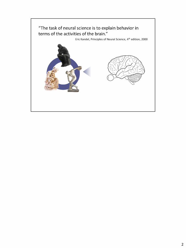
2

3

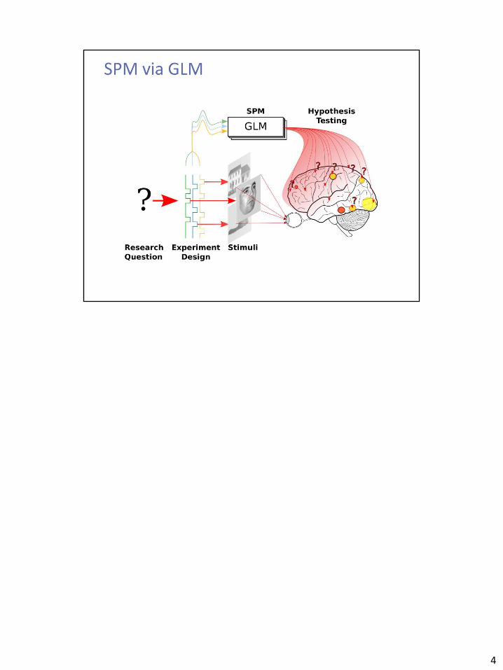
4

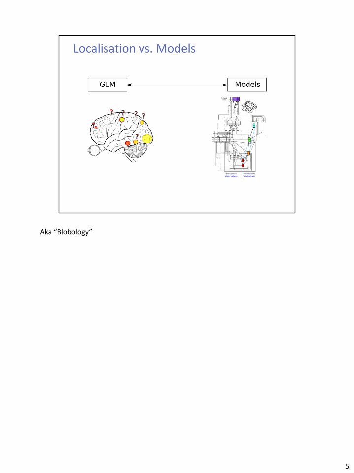
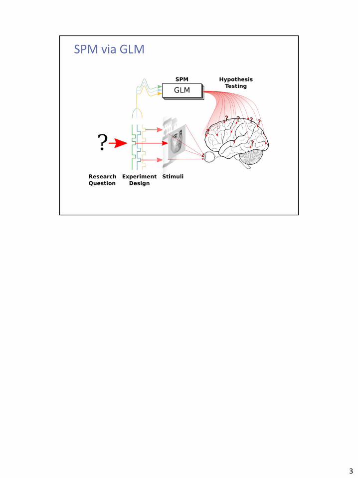
Aka “Blobology”

5

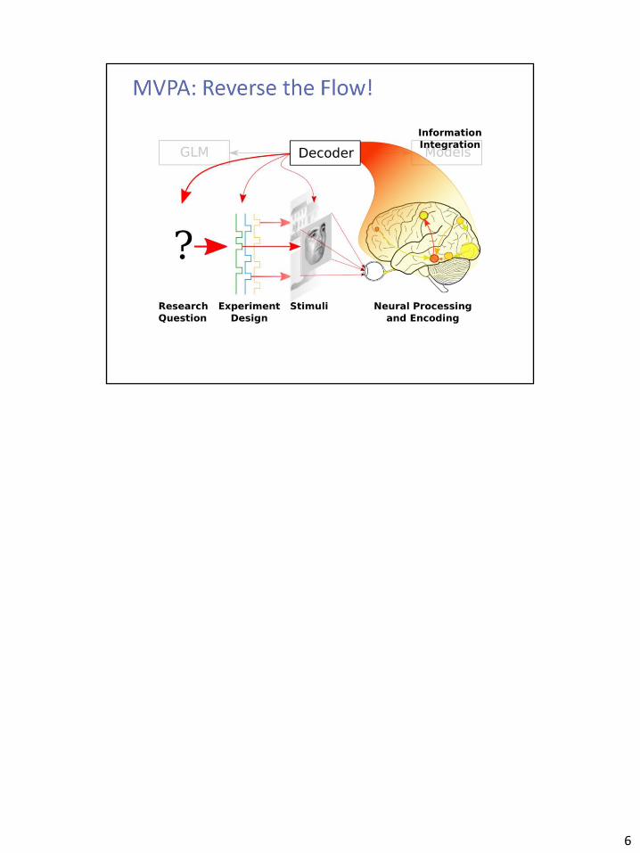
6

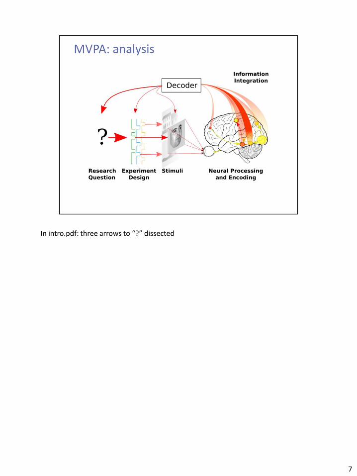
In intro.pdf: three arrows to “?” dissected

7

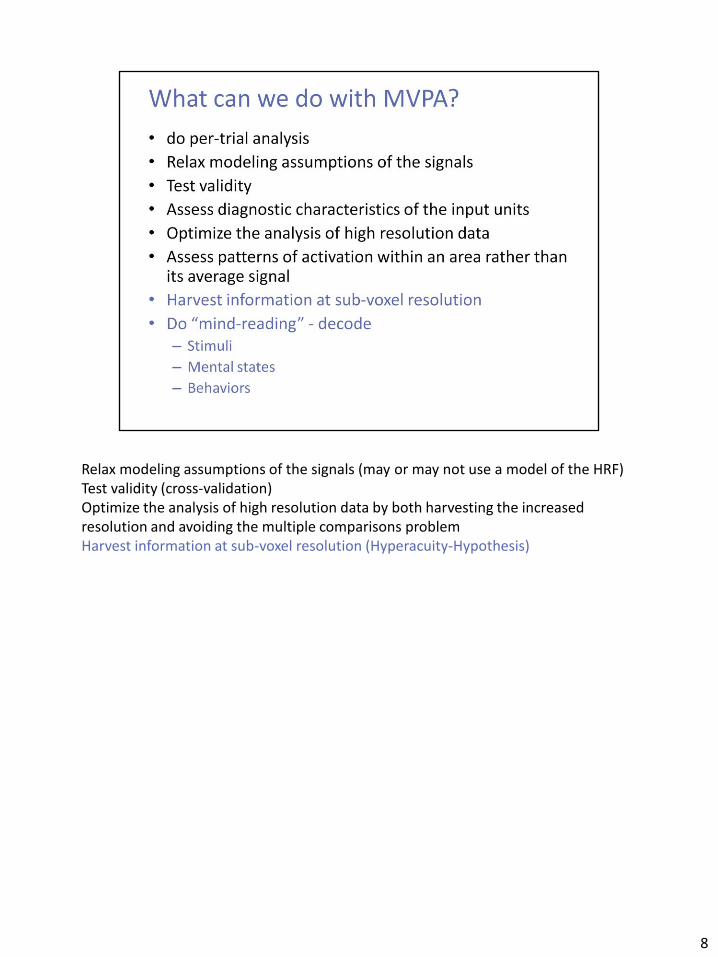
Relax modeling assumptions of the signals (may or may not use a model of the HRF) Test validity (cross-validation) Optimize the analysis of high resolution data by both harvesting the increased resolution and avoiding the multiple comparisons problem Harvest information at sub-voxel resolution (Hyperacuity-Hypothesis)

8

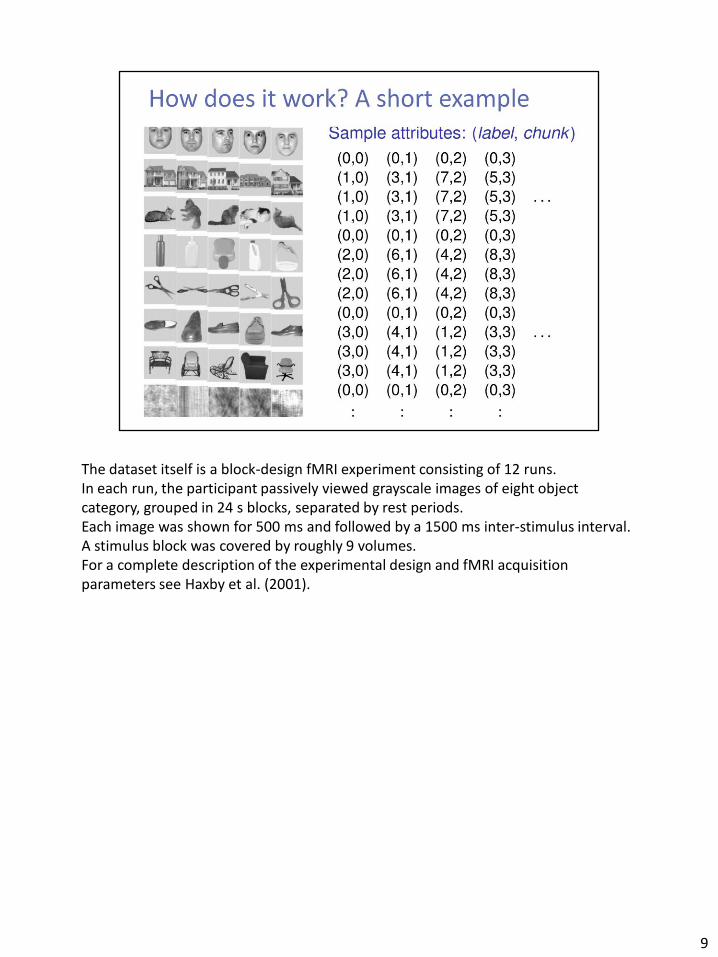
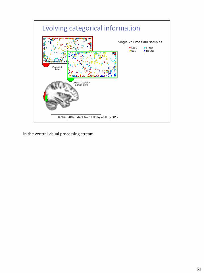
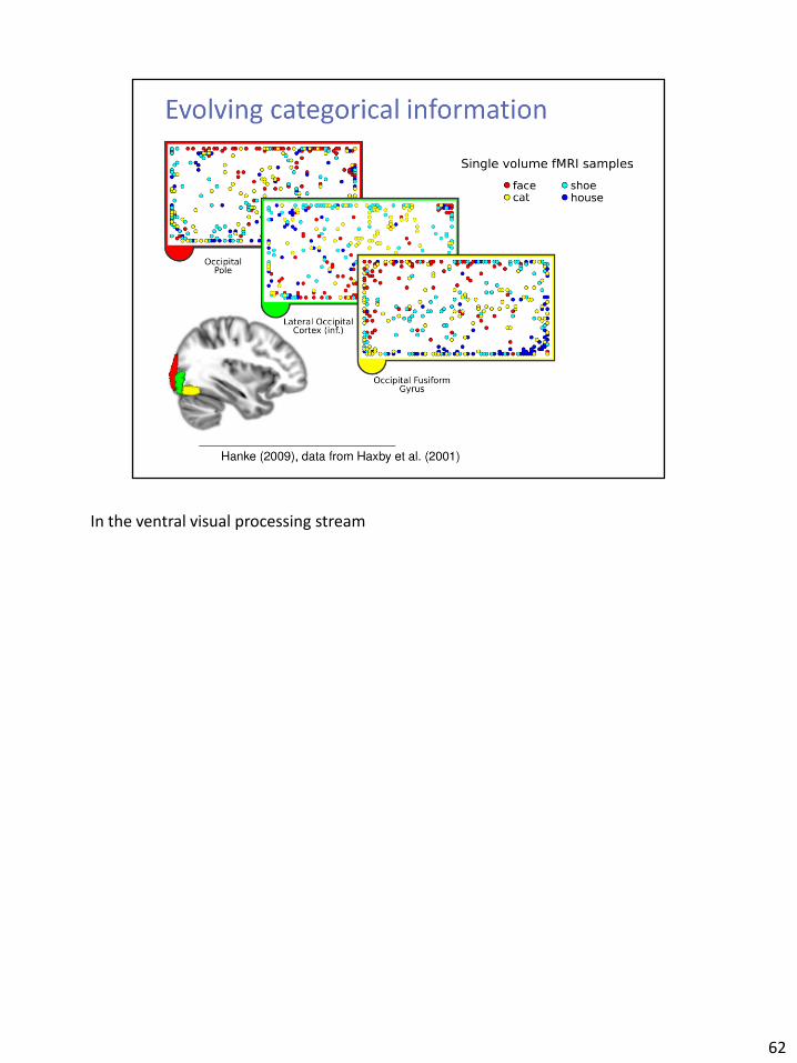
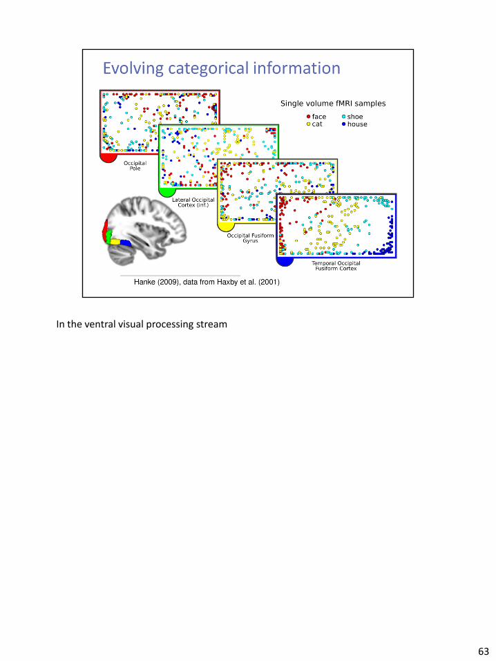
The dataset itself is a block-design fMRI experiment consisting of 12 runs. In each run, the participant passively viewed grayscale images of eight object category, grouped in 24 s blocks, separated by rest periods. Each image was shown for 500 ms and followed by a 1500 ms inter-stimulus interval. A stimulus block was covered by roughly 9 volumes. For a complete description of the experimental design and fMRI acquisition parameters see Haxby et al. (2001).

9

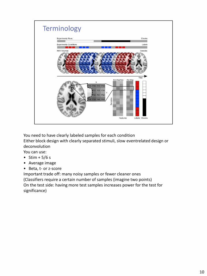
You need to have clearly labeled samples for each condition Either block design with clearly separated stimuli, slow eventrelated design or deconvolution You can use: • Stim + 5/6 s • Average image • Beta, t- or z-score Important trade off: many noisy samples or fewer cleaner ones (Classifiers require a certain number of samples (imagine two points) On the test side: having more test samples increases power for the test for significance)

10

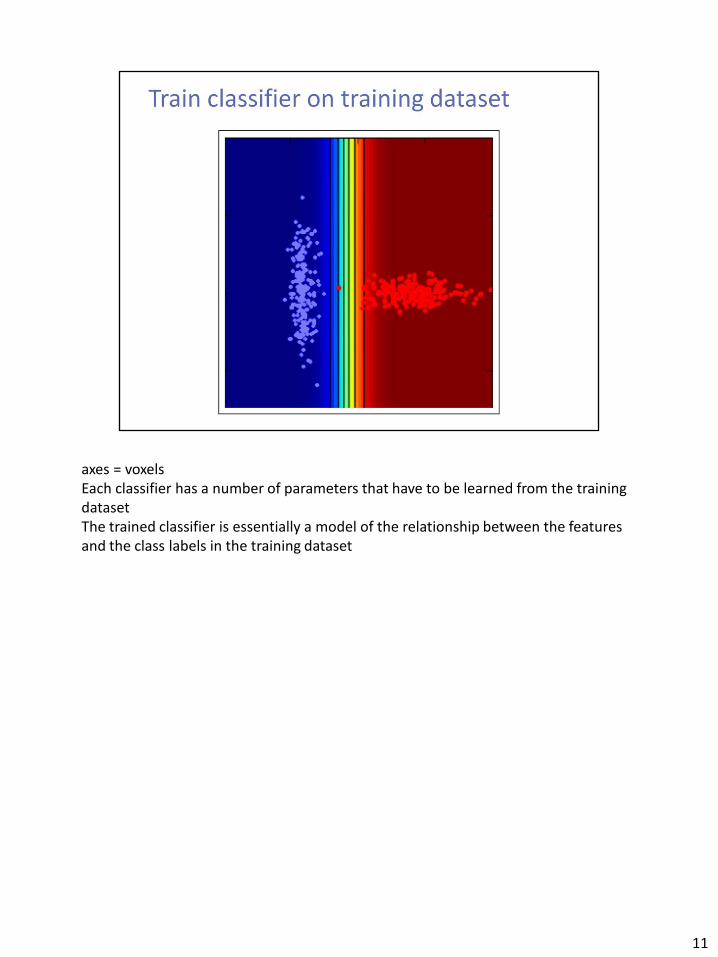
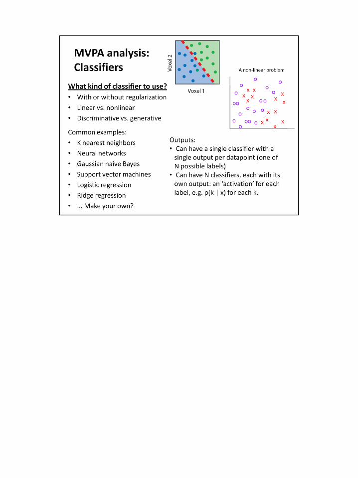
axes = voxels Each classifier has a number of parameters that have to be learned from the training dataset The trained classifier is essentially a model of the relationship between the features and the class labels in the training dataset

11

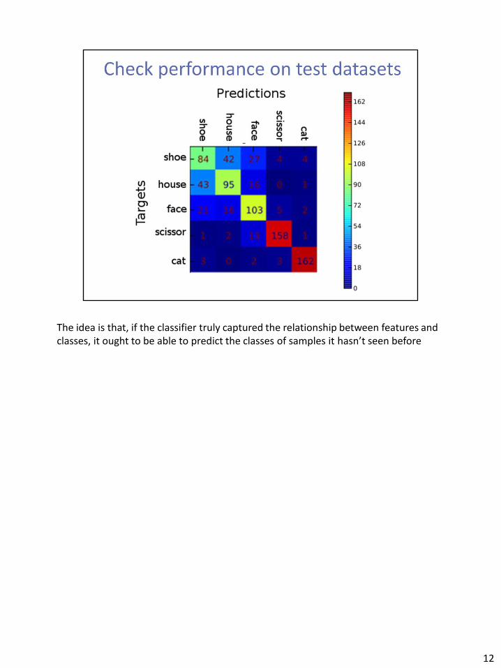
The idea is that, if the classifier truly captured the relationship between features and classes, it ought to be able to predict the classes of samples it hasn’t seen before

12

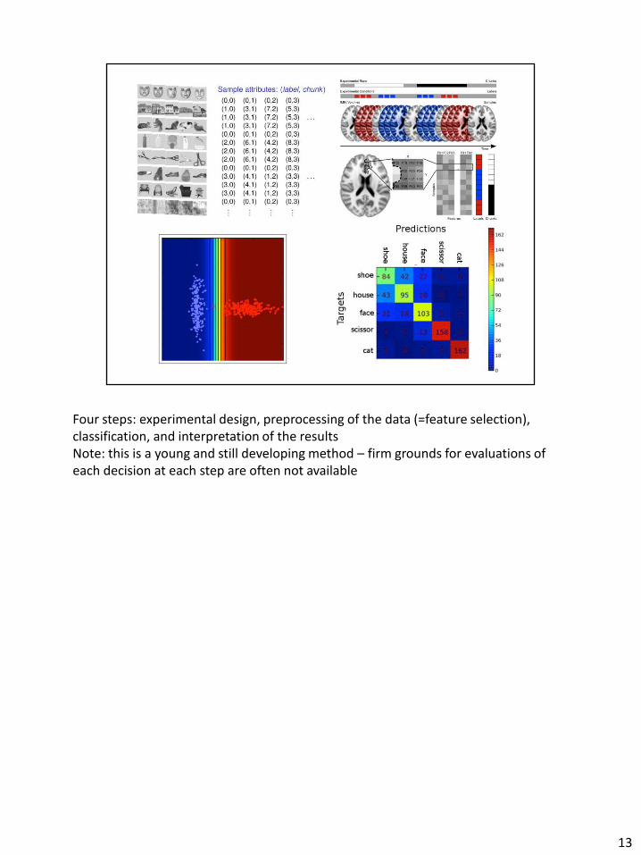
Four steps: experimental design, preprocessing of the data (=feature selection), classification, and interpretation of the results Note: this is a young and still developing method – firm grounds for evaluations of each decision at each step are often not available

13

14

15

one condition per TR: the default? can probably handle different stuff. but If you want your ‘face’ classifier to tell you how much a person is thinking about faces at a given time.

19

23

Over-fitting: fitting to noise.

- (Leave-one-out) cross-validation: Split up your data into N equally sized chunks. Leave out one chunk as your test set, then train on the rest. Iterate through all N chunks. - Cross-validation. Don’t have to “waste” any of your data. Can train on more of it. Iterate through so that you aren’t biased by any particular chunks. - Other kinds of cross-validation: odd-even.

- Occam’s razor. The simplest solution is the truest one.

Over-fitting: fitting to noise.

- (Leave-one-out) cross-validation: Split up your data into N equally sized chunks. Leave out one chunk as your test set, then train on the rest. Iterate through all N chunks. - Cross-validation. Don’t have to “waste” any of your data. Can train on more of it. Iterate through so that you aren’t biased by any particular chunks. - Other kinds of cross-validation: odd-even.

- Occam’s razor. The simplest solution is the truest one.

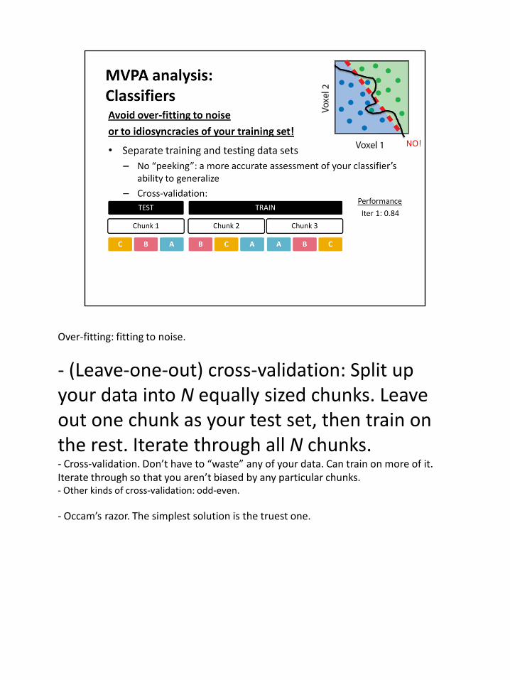
Over-fitting: fitting to noise.

- (Leave-one-out) cross-validation: Split up your data into N equally sized chunks. Leave out one chunk as your test set, then train on the rest. Iterate through all N chunks. - Cross-validation. Don’t have to “waste” any of your data. Can train on more of it. Iterate through so that you aren’t biased by any particular chunks. - Other kinds of cross-validation: odd-even.

- Occam’s razor. The simplest solution is the truest one.

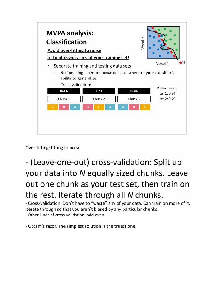
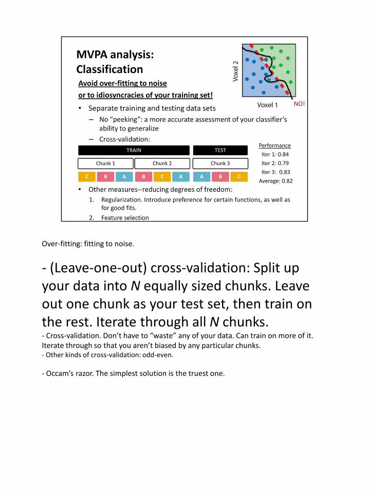
30

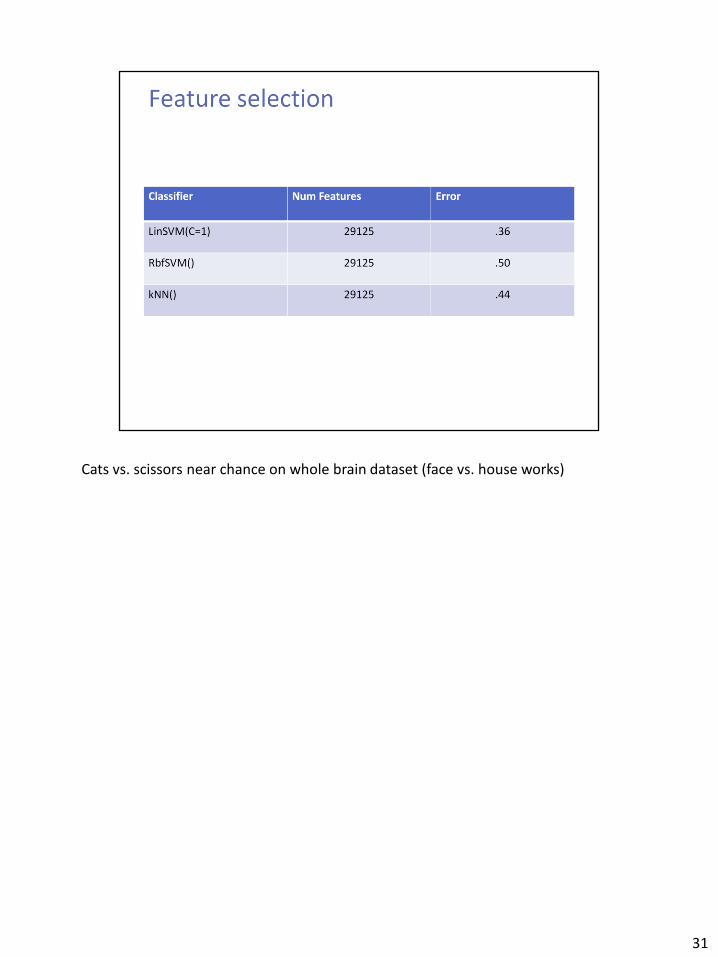
Cats vs. scissors near chance on whole brain dataset (face vs. house works)

31

Singular value decomposition, Independent Component Analysis: transform the original feature space (voxels) into a new, low-dimensional feature space Might reduce interpretability of your features (but is a necessary step for some classifiers)

32

Basic idea: scan the whole brain by automatically running as multiple ROI analyses In this analysis MVPA on spherical ROIs of a given radius centered around any voxel is done Afterwards, the resulting generalization error is plotted back onto the center voxel of the sphere, giving a whole brain generalization map A searchlight analysis will give you the power of MVPA while still being able to localize where the signal came from However, there are some limitations • You are restricting yourself of patterns from a small region of the brain, which is

somewhat contradictory to the idea of looking at distributed activation patterns underlying a cognitive function (but performs well if the target signal is in a spatially restricted area)

• Integrating information across different anatomical and structural regions, problems at the outer voxels (so, flattening the brain surface before doing any analyses would be a good idea)

• Reintroducing the the problem of multiple comparisons

33

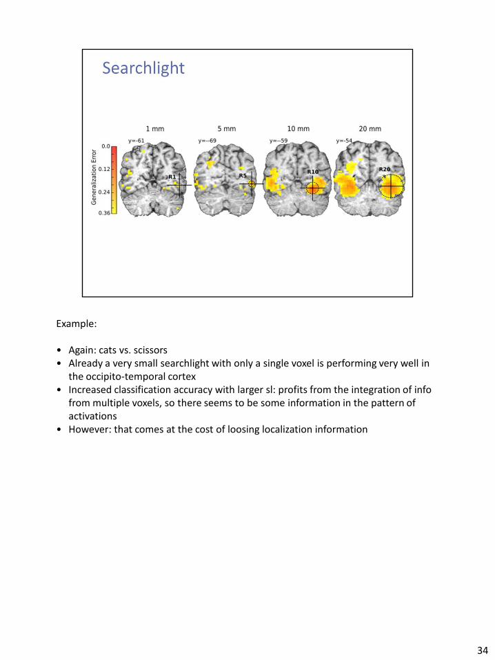
Example:

• Again: cats vs. scissors • Already a very small searchlight with only a single voxel is performing very well in

the occipito-temporal cortex • Increased classification accuracy with larger sl: profits from the integration of info

from multiple voxels, so there seems to be some information in the pattern of activations

• However: that comes at the cost of loosing localization information

34

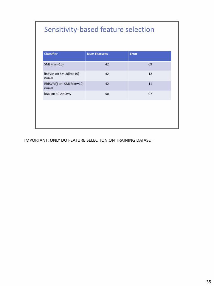
IMPORTANT: ONLY DO FEATURE SELECTION ON TRAINING DATASET

35

IF YOU DO ALL OF THE ABOVE, YOU WILL HAVE TO DO BONFERRONI CORRECTION

36

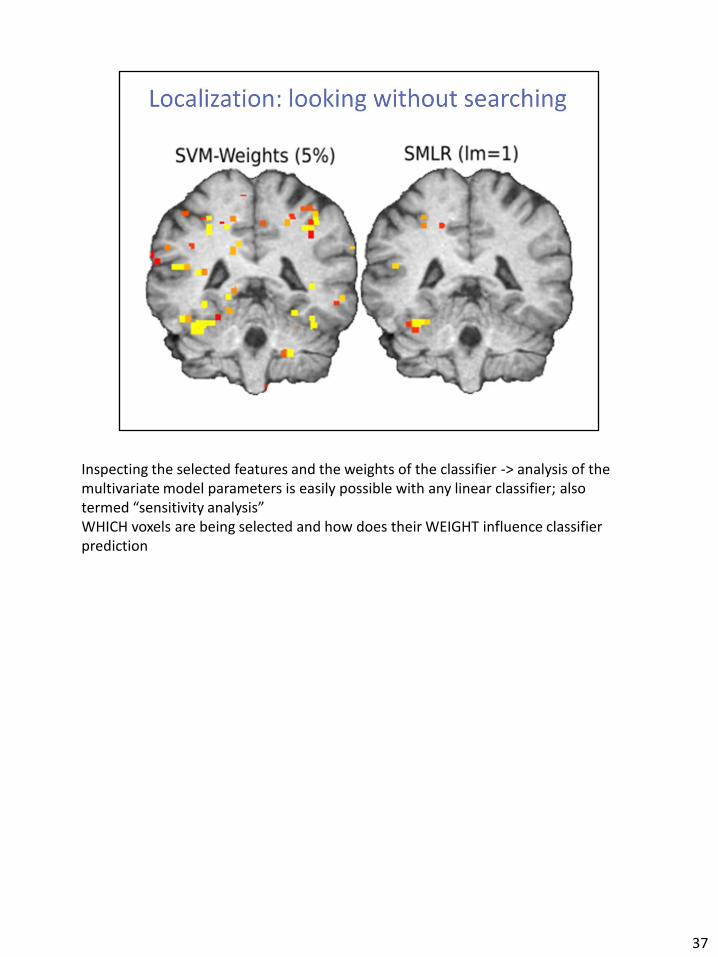
Inspecting the selected features and the weights of the classifier -> analysis of the multivariate model parameters is easily possible with any linear classifier; also termed “sensitivity analysis” WHICH voxels are being selected and how does their WEIGHT influence classifier prediction

37

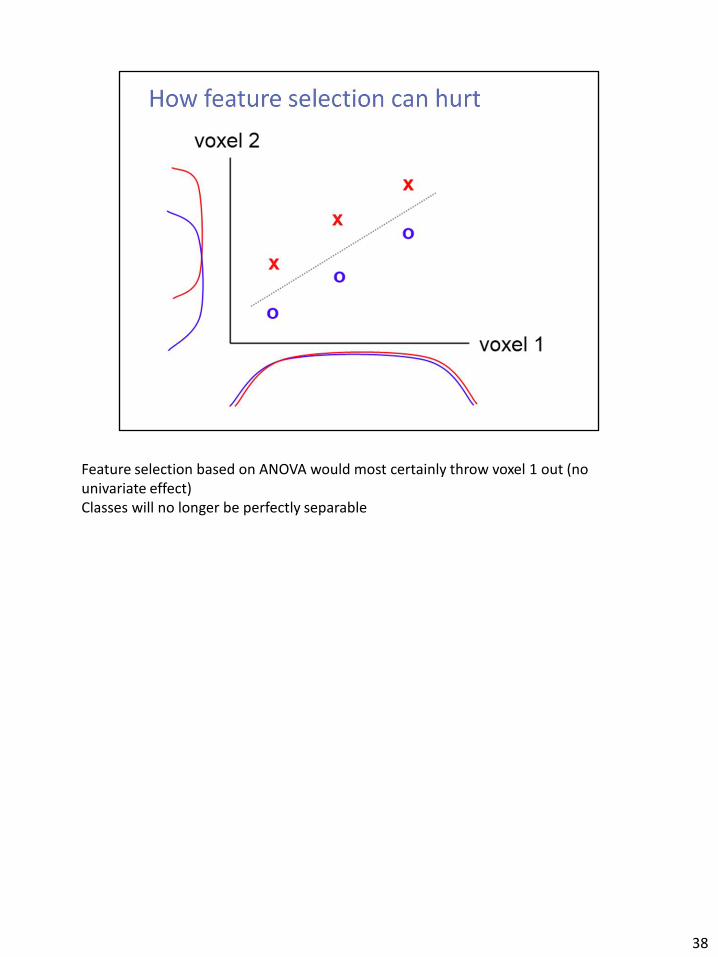
Feature selection based on ANOVA would most certainly throw voxel 1 out (no univariate effect) Classes will no longer be perfectly separable

38

39

40

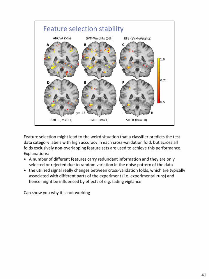
Feature selection might lead to the weird situation that a classifier predicts the test data category labels with high accuracy in each cross-validation fold, but across all folds exclusively non-overlapping feature sets are used to achieve this performance. Explanations: • A number of different features carry redundant information and they are only

selected or rejected due to random variation in the noise pattern of the data • the utilized signal really changes between cross-validation folds, which are typically

associated with different parts of the experiment (i.e. experimental runs) and hence might be influenced by effects of e.g. fading vigilance

Can show you why it is not working

41

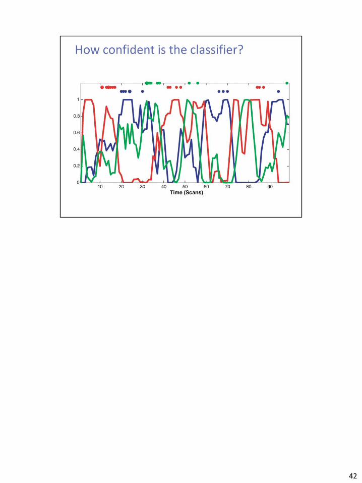
42

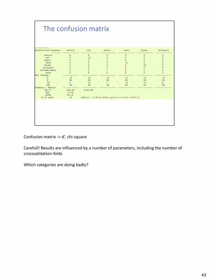
Confusion matrix -> d’, chi-square Carefull! Results are influenced by a number of parameters, including the number of crossvalidation-folds Which categories are doing badly?

43

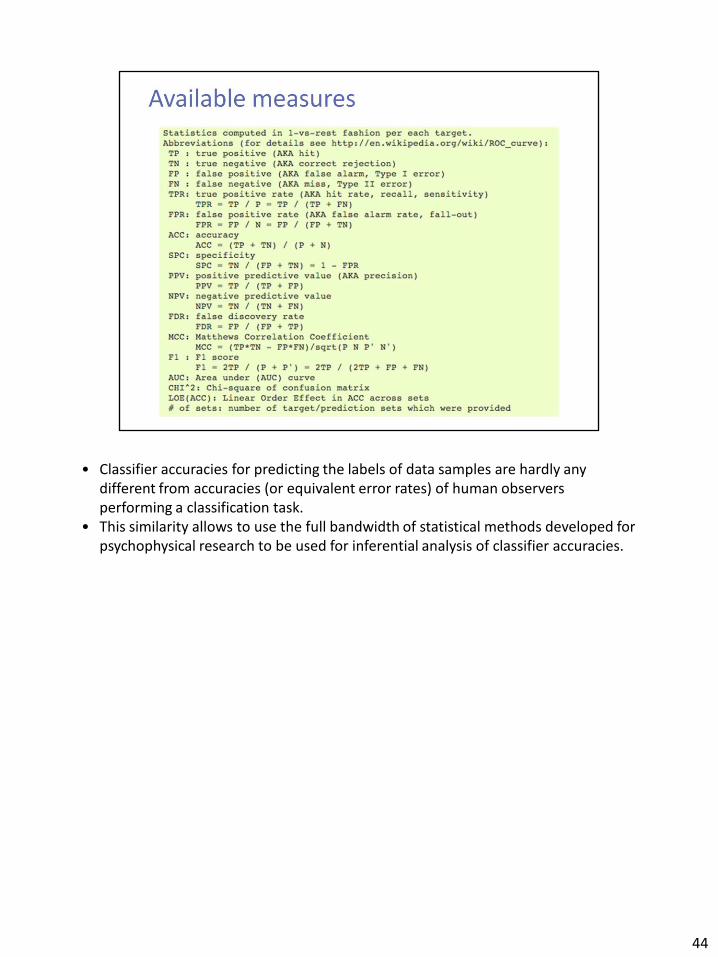
• Classifier accuracies for predicting the labels of data samples are hardly any different from accuracies (or equivalent error rates) of human observers performing a classification task.

• This similarity allows to use the full bandwidth of statistical methods developed for psychophysical research to be used for inferential analysis of classifier accuracies.

44

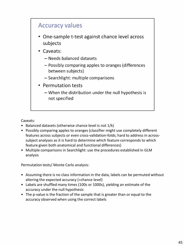
Caveats: • Balanced datasets (otherwise chance level is not 1/k) • Possibly comparing apples to oranges (classifier might use completely different

features across subjects or even cross-validation-folds; hard to address in across-subject analyses as it is hard to determine which feature corresponds to which feature given both anatomical and functional differences)

• Multiple comparisons in Searchlight: use the procedures established in GLM analysis

Permutation tests/ Monte Carlo analysis: • Assuming there is no class information in the data, labels can be permuted without

altering the expected accuracy (=chance level) • Labels are shuffled many times (100s or 1000s), yielding an estimate of the

accuracy under the null hypothesis • The p-value is the fraction of the sample that is greater than or equal to the

accuracy observed when using the correct labels

45

46

47

48

Include packages for stimulus generation, data acquisiton, data analysis, and visualization

49

Per Sederberg, Michael Hanke, Yaroslav Halchenko

50

51

52

Complete Documentation including a step-by-step tutorial can be found at pymvpa.org

53

54

55

56

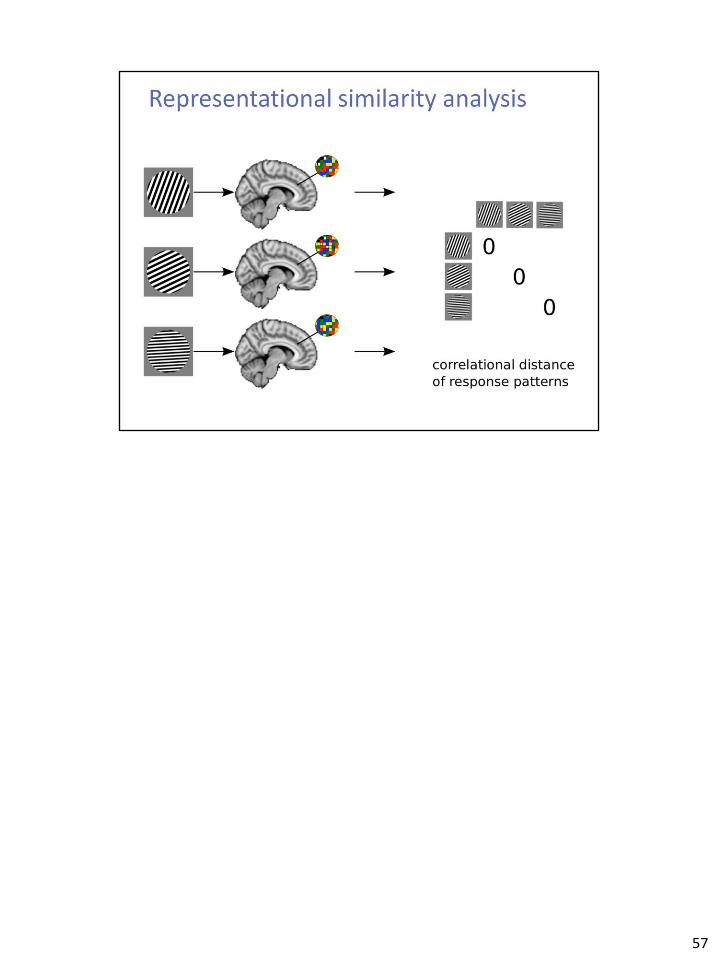
57

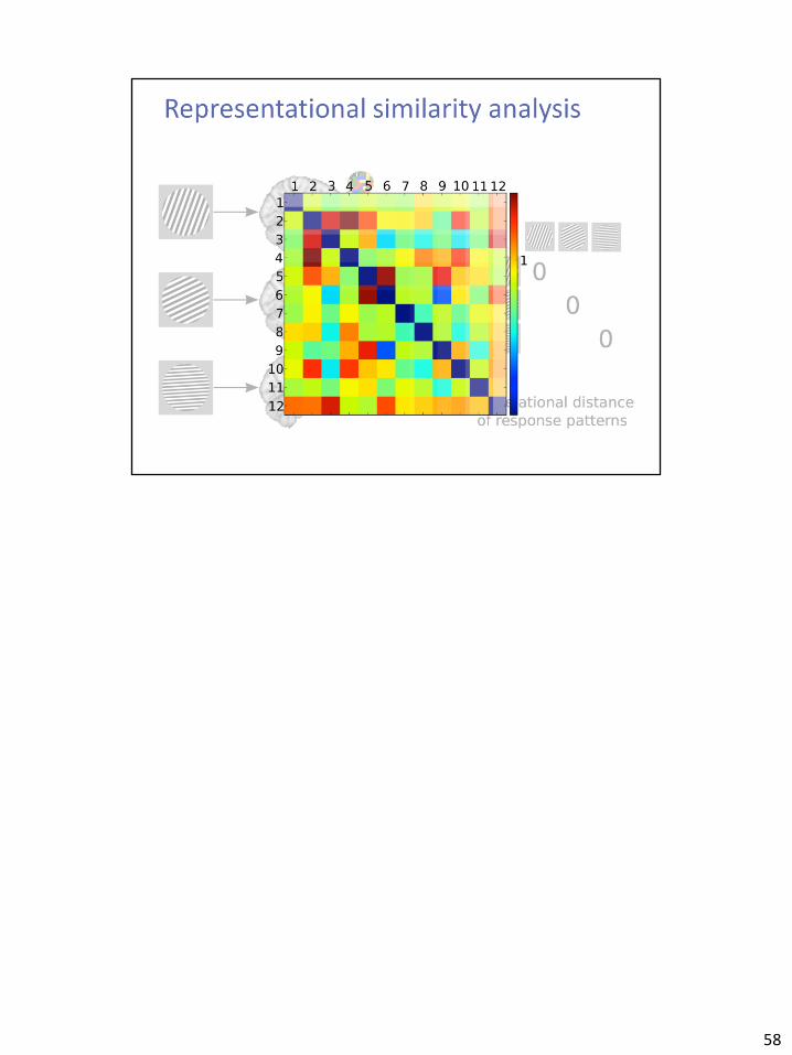
58

59

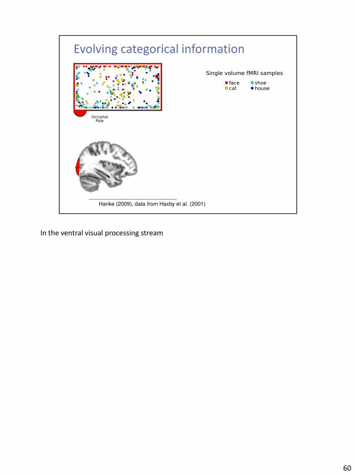
In the ventral visual processing stream

60

In the ventral visual processing stream

61

In the ventral visual processing stream

62

In the ventral visual processing stream

63

65