Embed Size (px)
Citation preview

Multivariate Regression
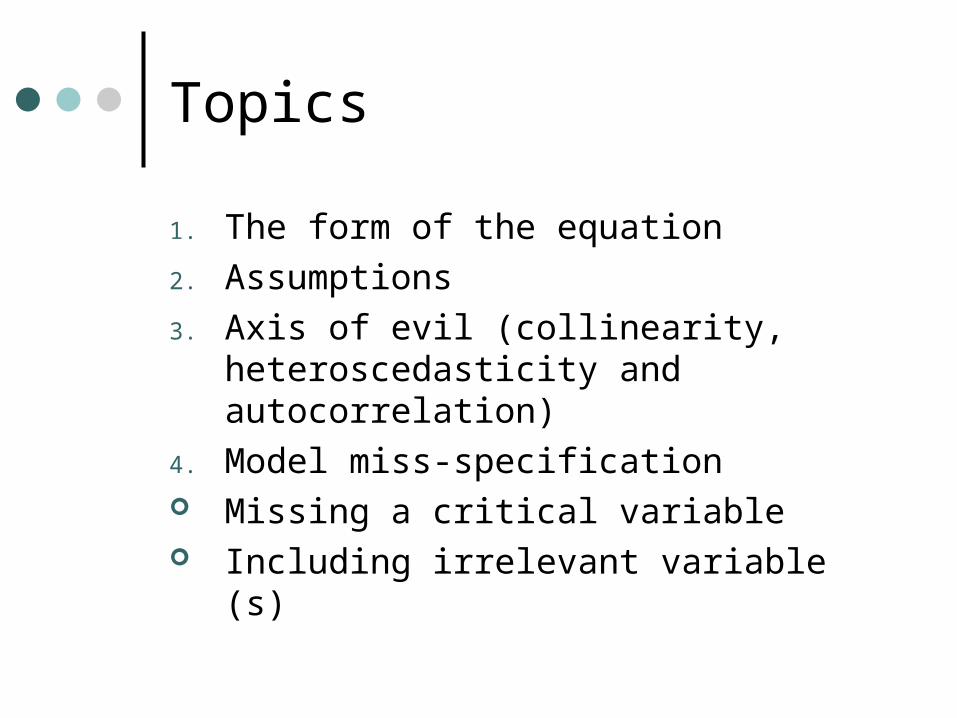
Topics
1. The form of the equation
2. Assumptions
3. Axis of evil (collinearity, heteroscedasticity and autocorrelation)
4. Model miss-specification Missing a critical variable Including irrelevant variable (s)
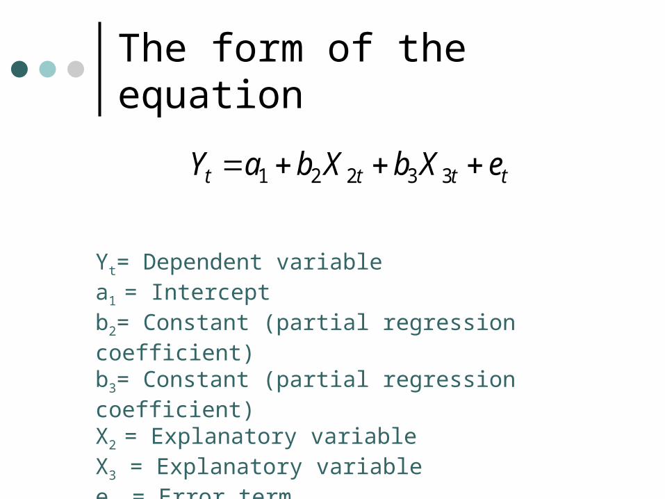
The form of the equation
tttt eXbXbaY 33221
Yt= Dependent variable a1 = Intercept b2= Constant (partial regression coefficient) b3= Constant (partial regression coefficient) X2 = Explanatory variableX3 = Explanatory variableet = Error term
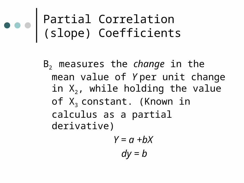
Partial Correlation (slope) Coefficients
B2 measures the change in the mean value of Y per unit change in X2, while holding the value of X3 constant. (Known in calculus as a partial derivative)
Y = a +bX
dy = b
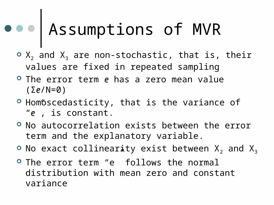
Assumptions of MVR
X2 and X3 are non-stochastic, that is, their values are fixed in repeated sampling
The error term ee has a zero mean value (Σee/N=0) Homoscedasticity, that is the variance of “ee”, is
constant. No autocorrelation exists between the error term
and the explanatory variable. No exact collinearity exist between X2 and X3
The error term “e” follows the normal distribution with mean zero and constant variance

Venn Diagram: Correlation & Coefficients of Determination (R2)
Y
X1 X2
No correlation exists betweenX1 and X2. Each variable explainsa portion of the variation of Y
Correlation exists betweenX1 and X2. There is a portion of thevariation of Y that can be attributed to either one
X1 X2
Y
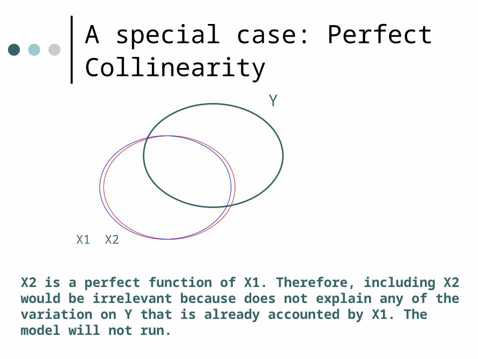
A special case: Perfect Collinearity
Y
X2 is a perfect function of X1. Therefore, including X2 would be irrelevant because does not explain any of the variation on Y that is already accounted by X1. The model will not run.
X1 X2
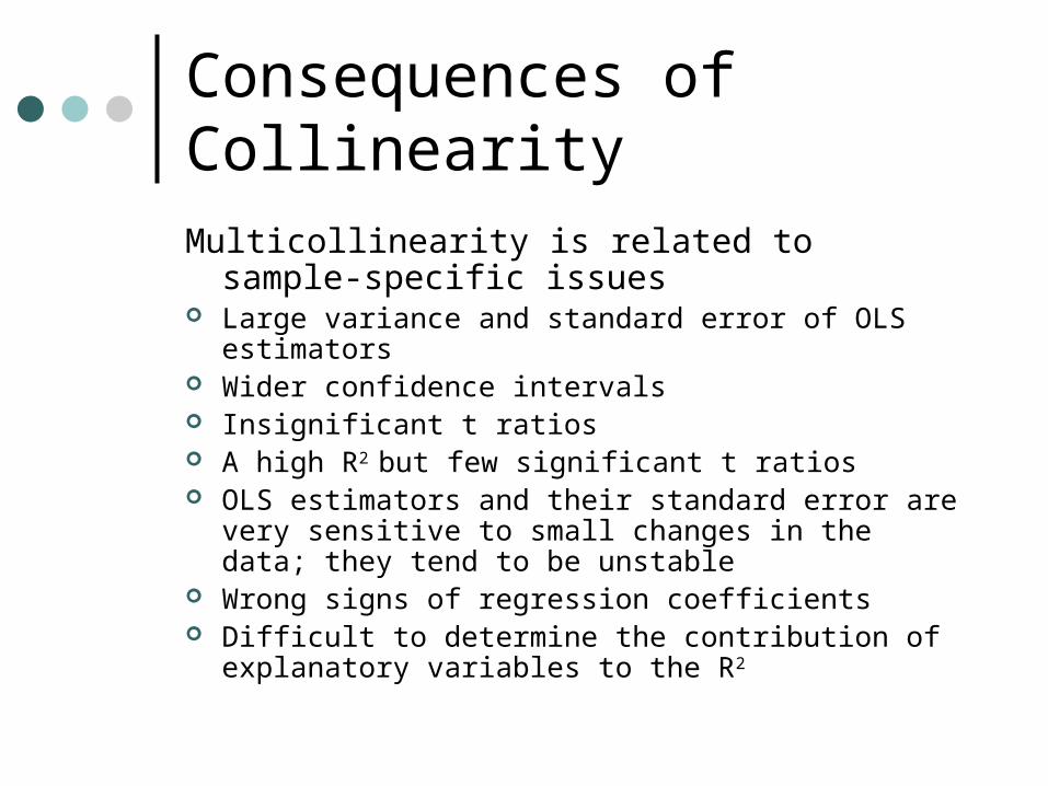
Consequences of CollinearityMulticollinearity is related to sample-specific
issues Large variance and standard error of OLS estimators Wider confidence intervals Insignificant t ratios A high R2 but few significant t ratios OLS estimators and their standard error are very
sensitive to small changes in the data; they tend to be unstable
Wrong signs of regression coefficients Difficult to determine the contribution of explanatory
variables to the R2
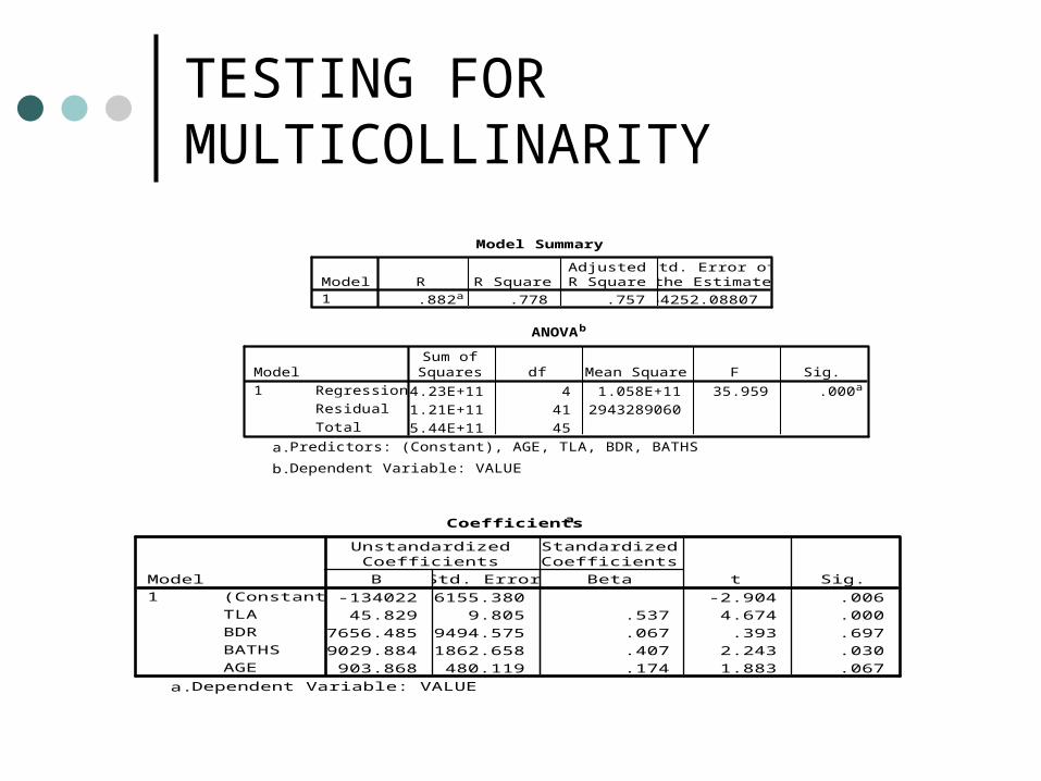
TESTING FOR MULTICOLLINARITY
Coefficientsa
-134022 46155.380 -2.904 .006
45.829 9.805 .537 4.674 .000
7656.485 19494.575 .067 .393 .697
49029.884 21862.658 .407 2.243 .030
903.868 480.119 .174 1.883 .067
(Constant)
TLA
BDR
BATHS
AGE
Model1
B Std. Error
UnstandardizedCoefficients
Beta
StandardizedCoefficients
t Sig.
Dependent Variable: VALUEa.
Model Summary
.882a .778 .757 54252.08807Model1
R R SquareAdjustedR Square
Std. Error ofthe Estimate
Predictors: (Constant), AGE, TLA, BDR, BATHSa. ANOVAb
4.23E+11 4 1.058E+11 35.959 .000a
1.21E+11 41 2943289060
5.44E+11 45
Regression
Residual
Total
Model1
Sum ofSquares df Mean Square F Sig.
Predictors: (Constant), AGE, TLA, BDR, BATHSa.
Dependent Variable: VALUEb.
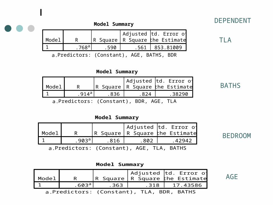
Model Summary
.768a .590 .561 853.81009Model1
R R SquareAdjustedR Square
Std. Error ofthe Estimate
Predictors: (Constant), AGE, BATHS, BDRa.
Model Summary
.914a .836 .824 .38290Model1
R R SquareAdjustedR Square
Std. Error ofthe Estimate
Predictors: (Constant), BDR, AGE, TLAa.
Model Summary
.903a .816 .802 .42942Model1
R R SquareAdjustedR Square
Std. Error ofthe Estimate
Predictors: (Constant), AGE, TLA, BATHSa.
Model Summary
.603a .363 .318 17.43586Model1
R R SquareAdjustedR Square
Std. Error ofthe Estimate
Predictors: (Constant), TLA, BDR, BATHSa.
TLA
BATHS
BEDROOM
AGE
DEPENDENT
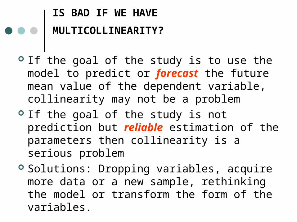
IS BAD IF WE HAVE MULTICOLLINEARITY?
If the goal of the study is to use the model to predict or forecast the future mean value of the dependent variable, collinearity may not be a problem
If the goal of the study is not prediction but reliable estimation of the parameters then collinearity is a serious problem
Solutions: Dropping variables, acquire more data or a new sample, rethinking the model or transform the form of the variables.
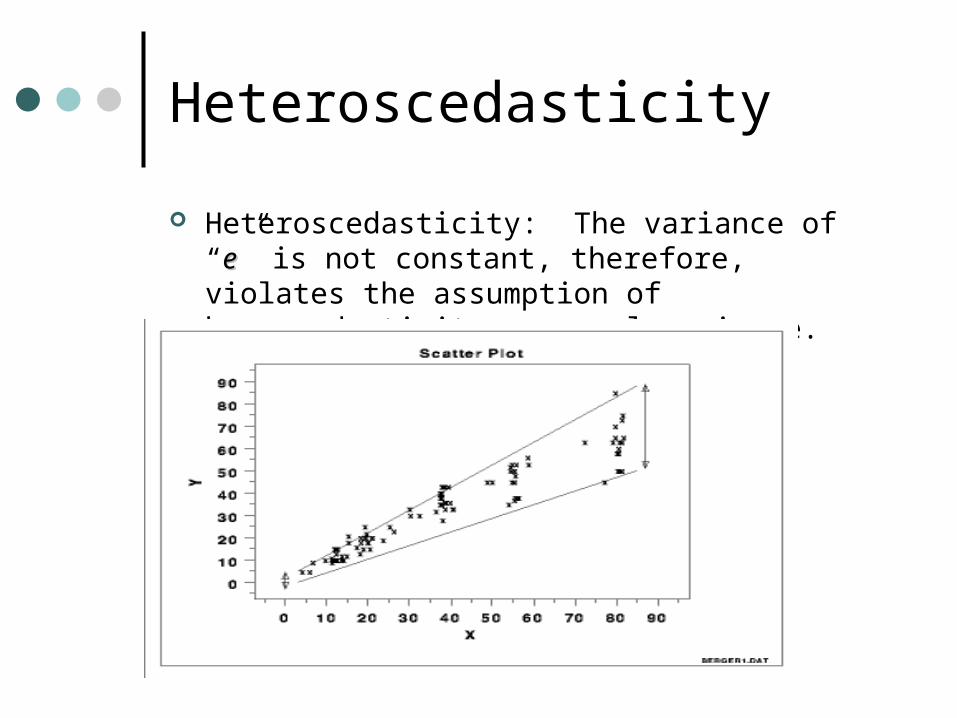
Heteroscedasticity
Heteroscedasticity: The variance of “ee” is not constant, therefore, violates the assumption of hemoscedasticity or equal variance.

Heteroscedasticity
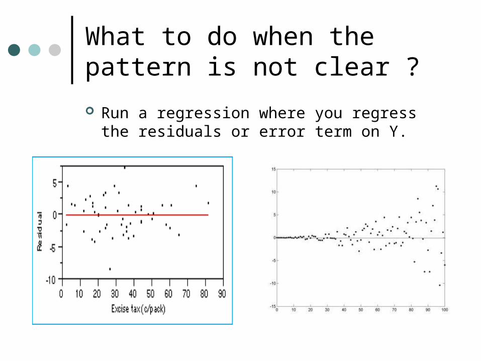
What to do when the pattern is not clear ?
Run a regression where you regress the residuals or error term on Y.
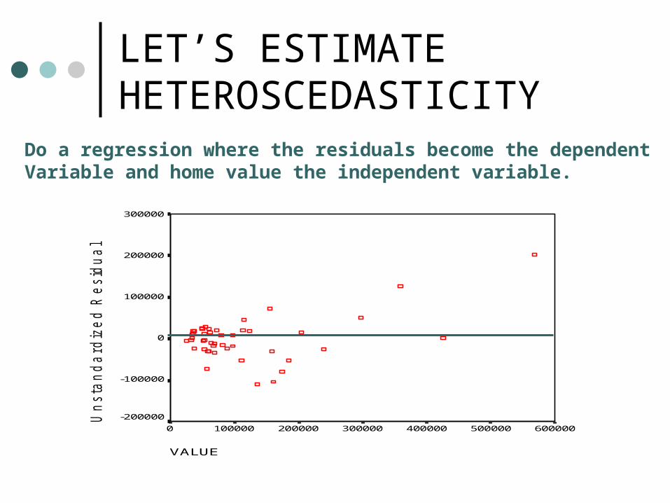
LET’S ESTIMATE HETEROSCEDASTICITY
VALUE
6000005000004000003000002000001000000
Un
sta
nd
ard
ize
d R
esid
ua
l
300000
200000
100000
0
-100000
-200000
Do a regression where the residuals become the dependentVariable and home value the independent variable.
Consequences of Heteroscedasticity
1. OLS estimators are still linear2. OLS estimators are still unbiased 3. But they no longer have minimum
variance. They are not longer BLUE4. Therefore we run the risk of drawing
wrong conclusions when doing hypothesis testing (Ho:b=0)
5. Solutions: variable transformation, develop a new model that takes into account no linearity (logarithmic function).

Testing for Heteroscedasticity
Unstandardized Predicted Value
5000004000003000002000001000000
LO
GR
ES
ID
11
10
9
8
7
6
Log e2
Let’s regress the predicted value (Y hat) on the log of the residual (log e2) to see the pattern of heteroscedasticity.
The above pattern shows that our relationships is best described as a Logarithmic function
Autocorrelation
Time-series correlation: The best predictor of sales for the present Christmas season is the previous Christmas season
Spatial correlation: The best predictor of a home’s value is the value of a home next door or in the same area or neighborhood.
The best predictor for a politician, to win an election as an incumbent, is the previous election (ceteris paribus)
Autocorrelation
Gujarati defines autocorrelation as “correlation between members of observations ordered in time [as time- series data] or space as [in cross-sectional data].
E (UiUj)=0 The product of two different error terms Ui and Uj is
zero. Autocorrelation is a model specification error
or the regression model is not specified correctly. A variable is missing or has the wrong functional form.
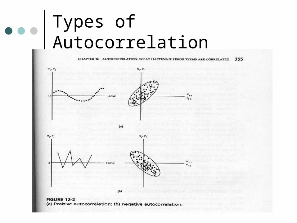
Types of Autocorrelation
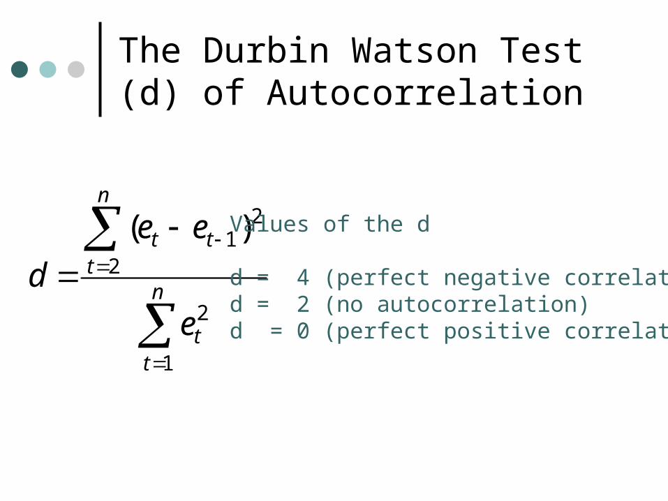
The Durbin Watson Test (d) of Autocorrelation
n
tt
t
n
tt
e
ee
d
1
2
21
2
)( Values of the d
d = 4 (perfect negative correlationd = 2 (no autocorrelation)d = 0 (perfect positive correlation)
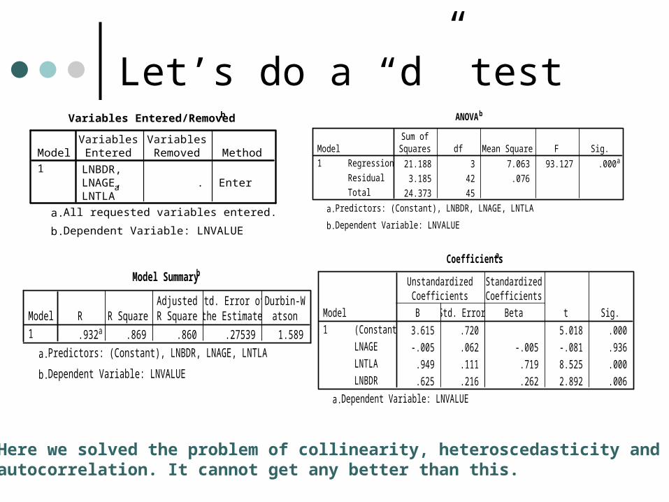
Let’s do a “d” test
Model Summaryb
.932a .869 .860 .27539 1.589Model1
R R SquareAdjustedR Square
Std. Error ofthe Estimate
Durbin-Watson
Predictors: (Constant), LNBDR, LNAGE, LNTLAa.
Dependent Variable: LNVALUEb.
ANOVAb
21.188 3 7.063 93.127 .000a
3.185 42 .076
24.373 45
Regression
Residual
Total
Model1
Sum ofSquares df Mean Square F Sig.
Predictors: (Constant), LNBDR, LNAGE, LNTLAa.
Dependent Variable: LNVALUEb.
Coefficientsa
3.615 .720 5.018 .000
-.005 .062 -.005 -.081 .936
.949 .111 .719 8.525 .000
.625 .216 .262 2.892 .006
(Constant)
LNAGE
LNTLA
LNBDR
Model1
B Std. Error
UnstandardizedCoefficients
Beta
StandardizedCoefficients
t Sig.
Dependent Variable: LNVALUEa.
Variables Entered/Removedb
LNBDR,LNAGE,LNTLA
a . Enter
Model1
VariablesEntered
VariablesRemoved Method
All requested variables entered.a.
Dependent Variable: LNVALUEb.
Here we solved the problem of collinearity, heteroscedasticity and autocorrelation. It cannot get any better than this.
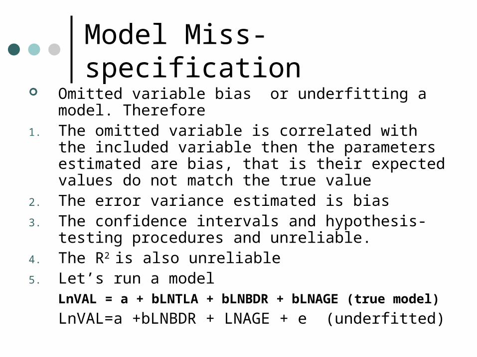
Model Miss-specification Omitted variable bias or underfitting a model.
Therefore1. The omitted variable is correlated with the included
variable then the parameters estimated are bias, that is their expected values do not match the true value
2. The error variance estimated is bias 3. The confidence intervals and hypothesis-testing
procedures and unreliable.4. The R2 is also unreliable 5. Let’s run a model
LnVAL = a + bLNTLA + bLNBDR + bLNAGE (true model)
LnVAL=a +bLNBDR + LNAGE + e (underfitted)
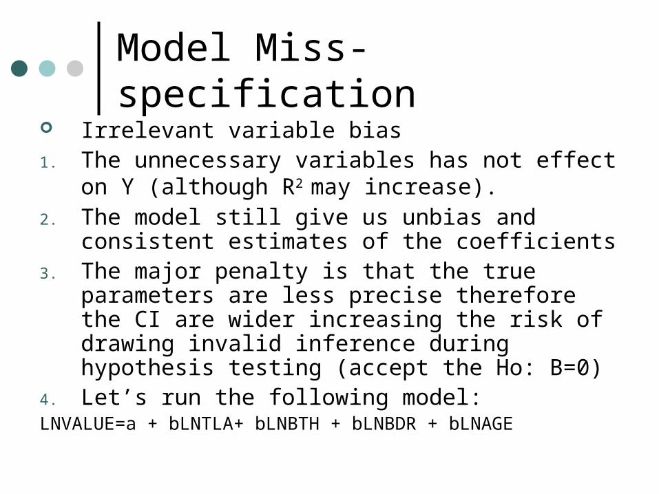
Model Miss-specification Irrelevant variable bias1. The unnecessary variables has not effect on Y
(although R2 may increase).
2. The model still give us unbias and consistent estimates of the coefficients
3. The major penalty is that the true parameters are less precise therefore the CI are wider increasing the risk of drawing invalid inference during hypothesis testing (accept the Ho: B=0)
4. Let’s run the following model:LNVALUE=a + bLNTLA+ bLNBTH + bLNBDR + bLNAGE