NeuroImage 56 (2011) 422–439

Contents lists available at ScienceDirect

NeuroImage

j ourna l homepage: www.e lsev ie r.com/ locate /yn img

Multivariate models of inter-subject anatomical variability

John Ashburner a,⁎, Stefan Klöppel b

a Wellcome Trust Centre for Neuroimaging, 12 Queen Square, London, WC1N 3BG, UKb Department of Psychiatry and Psychotherapy, Section of Gerontopsychiatry and Neuropsychology, Freiburg Brain Imaging, University Hospital Freiburg, Freiburg, Germany

⁎ Corresponding author. Fax: +44 20 78131420.

doi:10.1016/j.neuroimage.2010.03.0591053-8119 © 201 Elsevier Inc. Open access under CC BY0

a b s t r a c t

a r t i c l e i n f o

Article history:Received 30 October 2009Revised 22 January 2010Accepted 19 March 2010Available online 27 March 2010

This paper presents a very selective review of some of the approaches for multivariate modelling of inter-subject variability among brain images. It focusses on applying probabilistic kernel-based pattern recognitionapproaches to pre-processed anatomical MRI, with the aim of most accurately modelling the differencebetween populations of subjects. Some of the principles underlying the pattern recognition approaches ofGaussian process classification and regression are briefly described, although the reader is advised to lookelsewhere for full implementational details. Kernel pattern recognition methods require matrices thatencode the degree of similarity between the images of each pair of subjects. This review focusses onsimilarity measures derived from the relative shapes of the subjects' brains. Pre-processing is viewed asgenerative modelling of anatomical variability, and there is a special emphasis on the diffeomorphic imageregistration framework, which provides a very parsimonious representation of relative shapes. Although thereview is largely methodological, excessive mathematical notation is avoided as far as possible, as the paperattempts to convey a more intuitive understanding of various concepts. The paper should be of interest toreaders wishing to apply pattern recognition methods to MRI data, with the aim of clinical diagnosis orbiomarker development. It also tries to explain that the best models are those that most accurately predict,so similar approaches should also be relevant to basic science. Knowledge of some basic linear algebra andprobability theory should make the review easier to follow, although it may still have something to offer tothose readers whose mathematics may be more limited.

1 This was the maWant to See in Brain

license.

© 201 Elsevier Inc. Open access under CC BY license.0

Introduction

In recent years, the neuroimaging field has begun to see anincreasing popularity in the use of modelling approaches that aremultivariate over space. Rather than testing hypotheses aboutregionally specific effects using mass-univariate statistical models,such techniques attempt to combine all the data into the same model.Such an approach may be able to uncover unpredicted patterns thatcould otherwise be overlooked. The field of multivariate modelling isextremely large, so the current manuscript will be limited to a smallsubset of approaches for classification and regression. One particularstrategy for modelling inter-subject anatomical variability will also beemphasised. Practical real world applications of pattern recognitionmodels are obvious, but their contribution to our understanding ofneuroanatomical variability may be less clear, so a small section onvisualising differences is included.

Scientific research is usually dichotomised into the domains ofbasic (also known as fundamental or pure) and applied research. Morerecently, the concept of translational research has arisen withinbiomedical sciences, which is an alternative paradigm based upon amore seamless integration of the two traditionally separate domains

of basic and applied research. Many consider basic research as simply“not-yet-applied”, which broadly agrees with the mission statementsof the bodies that fund neuroimaging research.

When science is applied, it generally involves the use of models tomake predictions, where these predictions may inform some decisionmaking process. The ability to predict the behaviour of a systemshould enable interventions to be made that are more likely to causefavourable outcomes, where the favourability may be definedexplicitly according to some utility function. For example, in amedical situation the objective would be to treat the patient tooptimise life expectancy and quality of life measures, as well asfinancial and other considerations. Clinical intuition often conflictswith the optimal approach to decision making (Elstein and Schwarz,2002), although evidence based medicine prescribes the use of Bayestheorem in order to overcome the various cognitive biases. The abilityto predict is also useful for other translational areas such aspharmaceutical development, where decisions need to be made,such as those about which candidate drugs are most likely to succeed.One of the areas where brain imaging appears to offer the greatestpotential contribution to translation, is in the area of imagingbiomarkers.1 A useful imaging biomarker would have the ability to

in conclusion of the New York Academy of Sciences “What Do WeImaging?” meeting (London, UK. 3–4 December, 2007).

423J. Ashburner, S. Klöppel / NeuroImage 56 (2011) 422–439

predict the eventual outcome of treatment, before the final end pointcriterion is reached.

Biology is not an exact science, so ideally such predictions shouldbe probabilistic in order to encode the distribution of possible results.By predicting the probability over which events may occur, a model isalso saying which events ought not to occur, or are less probable.Model predictions are therefore needed to ensure that claims arefalsifiable. This paper will present a Bayesian perspective forvalidating claims, which involves comparing alternative models andselecting the one with the greatest evidence.

This journal is largely about basic neuroscience research, wherethe aim is to model the brain at the systems level. Having an accuratemodel of the system allows perturbations to be made to the model sothe effects of similar perturbations may be anticipated in the realworld. The usual aim of systems biology is to take a holistic view ofmodelling, which attempts to integrate data from a diverse range ofsources. The various “omics” techniques, form a key component ofsystems biology — along with the associated informatics and datamining procedures required for identifying hidden patterns in thedata (Kitano, 2002). Systems biology essentially involves an attemptto reverse engineer the system under study, where the end result is anaccurate and useful model (Markram, 2006). Typically, it takes severaldecades for basic research to become applied, and the development offully integrated models of the brain is still in the very tentative stages(Mazziotta et al., 2001; Oishi et al., 2008; Smith et al., 2009; Stephanet al., 2001). Every claim made by a scientist is in the context of somemodel or other, so findings pertaining to differences among popula-tions of subjects need to be interpreted within the context of a modelof inter-subject variability.

Many models can be thought of as generative models, as they allowsamples to be generated from the probability density they encode.Such samples may be considered as realisations of the data, assimulated by a Bayesian model. There are plenty of arguments infavour of adopting a Bayesian view of modelling. Through the use ofDutch Book arguments, Bruno de Finetti showed that the Bayesianprobabilistic framework provides the optimally coherent system forpredictive inference (see e.g. Jaynes and Bretthorst (2003)).Within deFinetti's framework, Bayesian models can be conceptualised as a wayof encoding probabilistic predictions about future observations, suchthat probabilities are represented over a whole range of possibleoutcomes. Probability densities learned by the models may be mademore “biologically plausible” by including realistic assumptions. Theseassumptions are largely derived empirically, but some aspects of goodmodels may be induced from first principles. For example, it is anecessary (but not sufficient) assumption that models should beformulated in a way that is internally consistent. Principles such assymmetry and invariance, which have played a large part in theinduction processes of physicists, may eventually become morecommonplace within other branches of science.

Currently, the scale of neuroimaging data is too large for acompletely coherent Bayesian generative model of inter-subjectvariability to be adopted. In practice, Bayesian modellers need tomake a number of assumptions in order to properly deal with theuncertainty with which parameters may be estimated. Even thesimplest of these approximations (the Laplace approximation) iscurrently too computationally expensive for the scale of modelneeded for anatomical MRI scans. However, such models are beingdeveloped for relatively small datasets (Allassonnière et al., 2007) andthe exponential growth in computer power may make them practicalwithin a few more years. Fully Bayesian generative models, such asDeep Belief Nets (Hinton et al., 2006), that currently work well withlots of two dimensional images of order 32×32,2 may eventuallybecome a reality for MRI data, which contain about 10,000 times as

2 See http://yann.lecun.com/exdb/mnist/ for the accuracy with which handwrittendigits can be recognized using various pattern recognition approaches.

many pixels. Until then though, a reasonable compromise is likely tobe from a feed-forward approach, where features are identified usingapproximate generative modelling strategies (i.e. not fully Bayesian),and these features are fed into a pattern recognition model.

There are several approaches that simply estimate the mostprobable values of model parameters, which are known asmaximum aposteriori (MAP) estimates. Although formulated from a generativemodelling perspective, they are not truly Bayesian because they donot properly consider the uncertainties of the parameter estimates.Modelling this uncertainty is necessary for making accurate probabi-listic predictions, or for making inferences about levels of significance.Currently, the most widely used data analysis strategy within theneuroimaging field involves using a series of models, such thatinformation derived from fitting a lower-level model is fed as inputinto the model at the next level. These models are colloquially knownas “tools”, and each application of a tool is a pre-processing step in ananalysis pipeline. The final step in the pipeline (the highest-levelmodel) is the one that answers the question posed by the investigator,which is often formulated within the SPM framework (Friston et al.,1994). In such approaches, information about the question of interestis not fed backwards into the pre-processing steps. For example, whenspatially normalising images prior to comparing a number ofpopulations of subjects, the scans would all be treated identicallyand aligned with the same template — irrespective of their groupmemberships. In principle, the effects that will later be modelled asconfounds in the general linear model could be fed back withoutbiasing the findings, but unless a fully Bayesian approach is adopted,including knowledge about effects of interest would lead to incorrectinferences.

Similar approaches will be described in this review, wherebyapproximate generative models are fitted to the original data in orderto capture useful lower-level features encoding inter-subject vari-ability. This is done without feedback from the top level, so there is noinfluence from information pertaining to the effects of interest.Features derived from this model are then entered into a completelyindependent pattern recognition scheme to characterise those aspectsof inter-subject variability that are of most interest to the investigator.

The paper is aimed at investigators who wish to model their data,but whose areas of expertise may lie elsewhere. Relatively littlemathematical notation is used, but appropriate references areprovided for those wishing to read further. Wherever possible, wehave attempted to explain the ideas in an intuitive way usinggraphical illustrations. The next section will describe some of theprinciples behind multivariate pattern recognition, but with anemphasis on probabilistic approaches. This will be followed by asection about some of the kinds of generative models that may beused for extracting features for use in multivariate modelling of inter-subject variability.

Multivariate pattern recognition

Many of the analyses of anatomical MRI data are carried out byclinical researchers, where the emphasis is often towards translationalor applied research. In many cases, the goal involves characterisingthe anatomical difference between two populations of subjects. Acommonly used approach is to localise volumetric differences ofparticular brain structures or tissue types, for example by using voxel-based morphometry (VBM) (Wright et al., 1995). Approaches such asthis allow the investigator to identify regions of significant differenceamong the pre-processed data. In the case of VBM, providing thetissue classification and inter-subject alignment models are suffi-ciently accurate, findings may be interpreted as regional volumetricdifferences (Ashburner and Friston, 2001).

Other ways of characterising differences exist (Petersson et al.,1999), which do not require the features to be discretely localised.Sometimes such characterisation may be formulated to answer

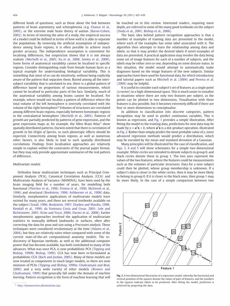
Fig. 1. A two dimensional illustration of a regression model, whereby the horizontal andvertical positions of the squares denote the values of pairs of features, and the numbers

424 J. Ashburner, S. Klöppel / NeuroImage 56 (2011) 422–439

different kinds of questions, such as those about the link betweenpatterns of brain asymmetry and schizophrenia (e.g. Chance et al.,2005), or the extreme male brain theory of autism (Baron-Cohen,2002). In terms of meeting the aims of a study, the empirical successof a model could be defined in terms of how well it is able to separatethe populations. By removing the artificial assumption of indepen-dence among brain regions, it is often possible to achieve muchgreater accuracy. The independence assumption is convenient forlocalising differences, but empiricism shows that it is not alwaysrealistic (Mechelli et al., 2005; Xu et al., 2008; Seeley et al., 2009).Some forms of anatomical variability cannot be localised to specificregions. Consider distinguishing male from female human faces as atypical example for understanding biological variability. This issomething that most of us can do intuitively, without being explicitlyaware of the pattern that separates them. Buried among all the inter-subject variability that is unrelated to sex, there is a global pattern ofdifference based on proportions of various measurements, whichcannot be localised to particular parts of the face. Similarly, much ofthe anatomical variability among brains cannot be localised. Forexample, where would one localise a pattern of difference where thetotal volume of the left hemisphere is inversely correlated with thevolume of the right hemisphere? Volumes of structures are correlatedamong different brain regions, especially between homotopic regionsin the contralateral hemisphere (Mechelli et al., 2005). Patterns ofgrowth are partially predicted by patterns of gene expression, and thegene expression maps at, for example, the Allen Brain Atlas3 showspatially distributed patterns. Darwin noted that there is correlation ofgrowth in his Origin of Species, so such pleiotropic effects should beexpected. Connectivity among brain regions, as well as numerousother factors, is also likely to lead to such spatially distributedcorrelations. Findings from localisation approaches are relativelysimple to explain within the constraints of the journal paper format,but they may only provide approximate summaries of the real patternof difference.

Multivariate models

Orthodox linear multivariate techniques such as Principal Com-ponent Analysis (PCA), Canonical Correlation Analysis (CCA) andMultivariate Analysis of Variance (MANOVA), have been used by thebrain imaging field for a number of years, for modelling bothfunctional (Fletcher et al., 1996; Friston et al., 1996; McIntosh et al.,1996) and structural (Bookstein, 1996; Ashburner et al., 1998) data.Similarly, morphometric applications of multivariate models haveexisted for many years, and there are several textbooks available onthe subject (Small, 1996; Bookstein, 1997; Dryden and Mardia, 1998;Kendall et al., 1999; da Fontoura Costa and Cesar, 2001; Lele andRichtsmeier, 2001; Krim and Yezzi, 2006; Davies et al., 2008). Earliermorphometric approaches involved the application of multivariatestatistics to manually defined landmarks or surfaces, often aftercorrecting the data for pose and size using a Procrustes analysis. Thesetechniques were considered revolutionary at the time (Adams et al.,2004), but they are relatively naïve when compared with some of thecurrent state-of-the-art computational anatomy models. The re-discovery of Bayesian methods, as well as the additional computerpower that has become available, has both contributed to many of theadvances. What was once PCA, is now probabilistic PCA (Tipping andBishop, 1999b; Bishop, 1999). CCA has now been re-formulated asprobabilistic CCA (Bach and Jordan, 2005). Many of these models arenow treated as components to much larger models, so there are nowmixtures of PCAs (Tipping and Bishop, 1999a; Ghahramani and Beal,2000) and a very wide variety of other models (Roweis andGhahramani, 1999) that generally fall under the domain of machinelearning. Pattern recognition is the form of machine learning that will

3 http://humancortex.alleninstitute.org/.

be touched on in this review. Interested readers, requiring moredepth, are referred to some of themany good textbooks on the subject(Duda et al., 2001; Bishop et al., 2006).

The basic idea behind pattern recognition approaches is that anumber of examples of training data are presented to the model,where each of the examples has some label associated with it. Thealgorithm then attempts to learn the relationship among data andlabels, so that it may predict the desired labels if novel examples ofdata are presented. A practical application may involve the data beingsome set of image features for each of a number of subjects, and thelabels may be either zero or one, depending on some disease status. Inthis situation, the model would attempt to automatically makediagnoses based on the image features of the new subjects. Similarapproaches have been used for functional data, for which introductoryand tutorial papers such as Mitchell et al. (2004) and Pereira et al.(2009) may be helpful.

It is useful to consider each subject's set of features as a single point(a vector) in a high-dimensional space. This is much easier to visualisein situations where there are only two features per subject, as thepoints can be plotted in two dimensions. Visualisation with threefeatures is also possible, but it becomes extremely difficult if there arefour or more dimensions to conceptualise.

In addition to classification into discrete categories, patternrecognition may be used to predict continuous variables. This isknown as regression, and Fig. 1 provides a simple illustration. Afterfitting the model to the training data, predictions for new data may bemade by y=aTx+b, where aTx is a dot-product operation, illustratedin Fig. 2. Rather than simply predict themost probable value of y, moreadvanced regression methods would predict a distribution, whichmay be encoded by the mean and standard deviation of a Gaussian.

Many principles will be illustrated for the case of classification, andFigs. 3, 4 and 5 will show schematics for a simple two dimensionalexample. White circles are intended to denote subjects in group 0, andblack circles denote those in group 1. The two axes represent thevalues of the two features, where the features could bemeasurementssuch as the volumes of particular structures. Data for a new subjectcould then be plotted, whose group membership is unknown. If asubject's data is closer to the white circles, then it may be more likelyto belong to group 0. If it is closer to the black ones, then group 1 maybe more likely. In the case of a simple comparison between two

in the squares indicate labels to be predicted. After fitting the model, prediction isachieved by projecting the data.

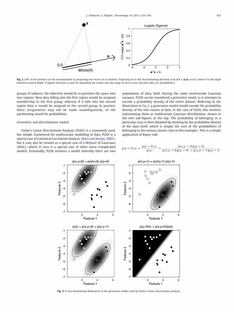
Fig. 2. Left: A dot-product can be conceptualised as projecting one vector on to another. Projecting on to the discriminating direction is by aTx=|a||x| cos(θ), where θ is the anglebetween a and x. Right: A logistic function is used for squashing the results into the range of zero to one (because they are probabilities).

425J. Ashburner, S. Klöppel / NeuroImage 56 (2011) 422–439

groups of subjects, the objective would be to partition the space intotwo regions. New data falling into the first region would be assignedmembership to the first group, whereas if it falls into the secondregion then it would be assigned to the second group. In practice,these assignments may not be made unambiguously, so thepartitioning would be probabilistic.

Generative and discriminative models

Fisher's Linear Discriminant Analysis (FLDA) is a commonly used,but simple, framework for multivariate modelling of data. FLDA is aspecial case of Canonical Correlation Analysis (Bach and Jordan, 2005),but it may also be viewed as a special case of a Mixture of Gaussians(MoG), which in turn is a special case of other more complicatedmodels. Essentially, FLDA involves a model whereby there are two

Fig. 3. A two dimensional illustration of the generative m

populations of data, both sharing the same multivariate Gaussianvariance. FLDA can be considered a generative model, as it attempts toencode a probability density of the entire dataset. Referring to theillustration in Fig 3, a generative model would encode the probabilitydensity of the two classes of data. In the case of FLDA, this involvesrepresenting them as multivariate Gaussian distributions, shown inthe two sub-figures at the top. The probability of belonging to aparticular class is then obtained by dividing by the probability densityof the data itself, which is simply the sum of the probabilities ofbelonging to the various classes (two in this example). This is a simpleapplication of Bayes rule:

p y = 0 jxð Þ = p y = 0;xð Þp xð Þ =

p x jy = 0ð Þp y = 0ð Þp x jy = 0ð Þp y = 0ð Þ + p x jy = 1ð Þp y = 1ð Þ :

odel used by Fisher's linear discriminant analysis.

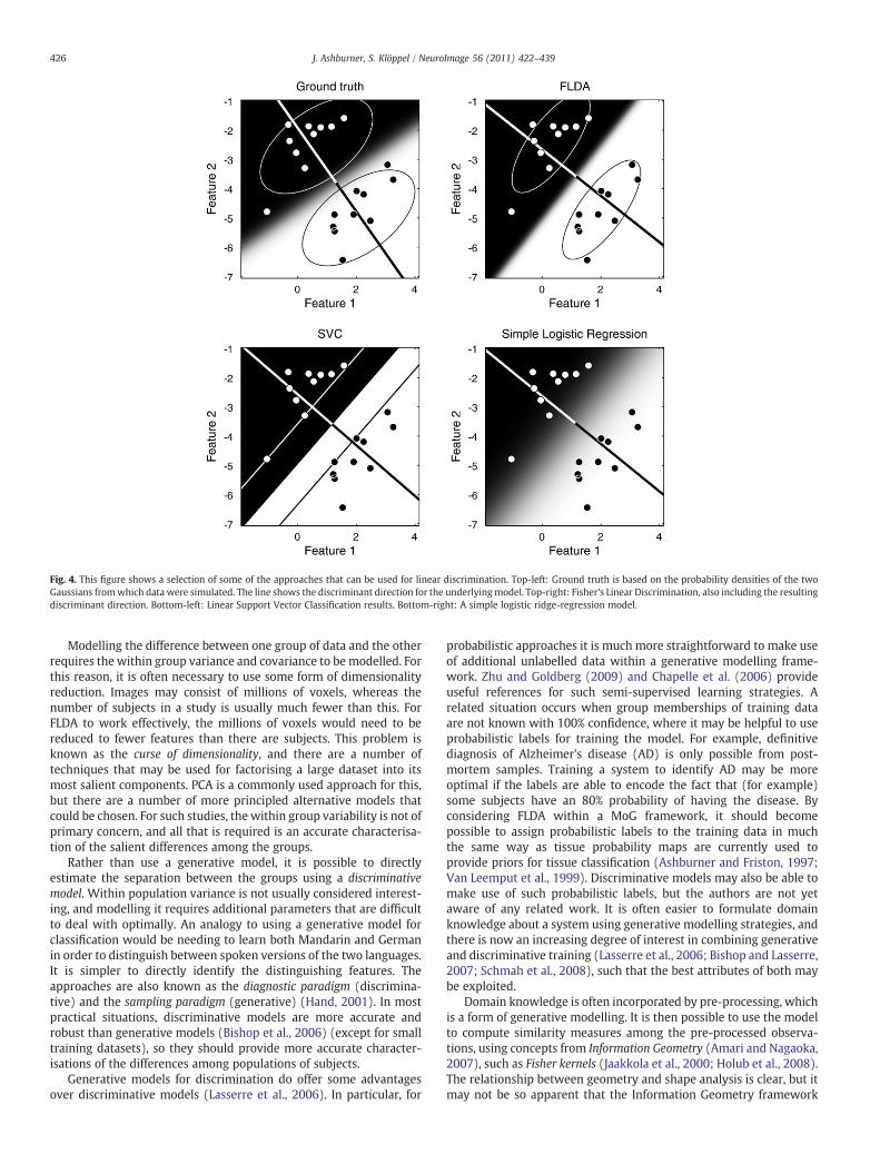
Fig. 4. This figure shows a selection of some of the approaches that can be used for linear discrimination. Top-left: Ground truth is based on the probability densities of the twoGaussians fromwhich data were simulated. The line shows the discriminant direction for the underlying model. Top-right: Fisher's Linear Discrimination, also including the resultingdiscriminant direction. Bottom-left: Linear Support Vector Classification results. Bottom-right: A simple logistic ridge-regression model.

426 J. Ashburner, S. Klöppel / NeuroImage 56 (2011) 422–439

Modelling the difference between one group of data and the otherrequires the within group variance and covariance to be modelled. Forthis reason, it is often necessary to use some form of dimensionalityreduction. Images may consist of millions of voxels, whereas thenumber of subjects in a study is usually much fewer than this. ForFLDA to work effectively, the millions of voxels would need to bereduced to fewer features than there are subjects. This problem isknown as the curse of dimensionality, and there are a number oftechniques that may be used for factorising a large dataset into itsmost salient components. PCA is a commonly used approach for this,but there are a number of more principled alternative models thatcould be chosen. For such studies, the within group variability is not ofprimary concern, and all that is required is an accurate characterisa-tion of the salient differences among the groups.

Rather than use a generative model, it is possible to directlyestimate the separation between the groups using a discriminativemodel. Within population variance is not usually considered interest-ing, and modelling it requires additional parameters that are difficultto deal with optimally. An analogy to using a generative model forclassification would be needing to learn both Mandarin and Germanin order to distinguish between spoken versions of the two languages.It is simpler to directly identify the distinguishing features. Theapproaches are also known as the diagnostic paradigm (discrimina-tive) and the sampling paradigm (generative) (Hand, 2001). In mostpractical situations, discriminative models are more accurate androbust than generative models (Bishop et al., 2006) (except for smalltraining datasets), so they should provide more accurate character-isations of the differences among populations of subjects.

Generative models for discrimination do offer some advantagesover discriminative models (Lasserre et al., 2006). In particular, for

probabilistic approaches it is much more straightforward to make useof additional unlabelled data within a generative modelling frame-work. Zhu and Goldberg (2009) and Chapelle et al. (2006) provideuseful references for such semi-supervised learning strategies. Arelated situation occurs when group memberships of training dataare not known with 100% confidence, where it may be helpful to useprobabilistic labels for training the model. For example, definitivediagnosis of Alzheimer's disease (AD) is only possible from post-mortem samples. Training a system to identify AD may be moreoptimal if the labels are able to encode the fact that (for example)some subjects have an 80% probability of having the disease. Byconsidering FLDA within a MoG framework, it should becomepossible to assign probabilistic labels to the training data in muchthe same way as tissue probability maps are currently used toprovide priors for tissue classification (Ashburner and Friston, 1997;Van Leemput et al., 1999). Discriminative models may also be able tomake use of such probabilistic labels, but the authors are not yetaware of any related work. It is often easier to formulate domainknowledge about a system using generative modelling strategies, andthere is now an increasing degree of interest in combining generativeand discriminative training (Lasserre et al., 2006; Bishop and Lasserre,2007; Schmah et al., 2008), such that the best attributes of both maybe exploited.

Domain knowledge is often incorporated by pre-processing, whichis a form of generative modelling. It is then possible to use the modelto compute similarity measures among the pre-processed observa-tions, using concepts from Information Geometry (Amari and Nagaoka,2007), such as Fisher kernels (Jaakkola et al., 2000; Holub et al., 2008).The relationship between geometry and shape analysis is clear, but itmay not be so apparent that the Information Geometry framework

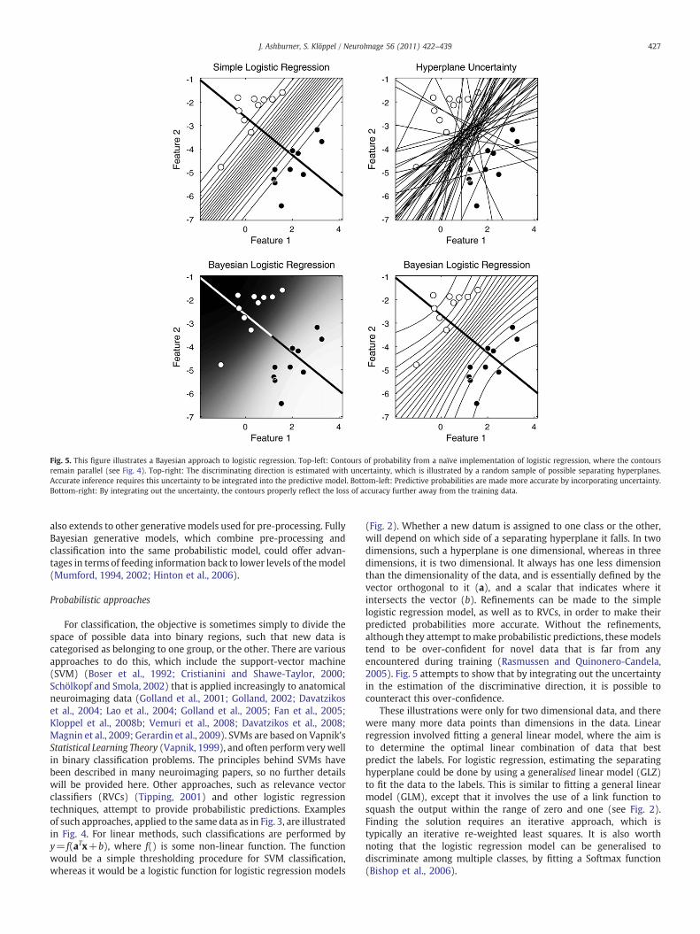
Fig. 5. This figure illustrates a Bayesian approach to logistic regression. Top-left: Contours of probability from a naïve implementation of logistic regression, where the contoursremain parallel (see Fig. 4). Top-right: The discriminating direction is estimated with uncertainty, which is illustrated by a random sample of possible separating hyperplanes.Accurate inference requires this uncertainty to be integrated into the predictive model. Bottom-left: Predictive probabilities are made more accurate by incorporating uncertainty.Bottom-right: By integrating out the uncertainty, the contours properly reflect the loss of accuracy further away from the training data.

427J. Ashburner, S. Klöppel / NeuroImage 56 (2011) 422–439

also extends to other generative models used for pre-processing. FullyBayesian generative models, which combine pre-processing andclassification into the same probabilistic model, could offer advan-tages in terms of feeding information back to lower levels of themodel(Mumford, 1994, 2002; Hinton et al., 2006).

Probabilistic approaches

For classification, the objective is sometimes simply to divide thespace of possible data into binary regions, such that new data iscategorised as belonging to one group, or the other. There are variousapproaches to do this, which include the support-vector machine(SVM) (Boser et al., 1992; Cristianini and Shawe-Taylor, 2000;Schölkopf and Smola, 2002) that is applied increasingly to anatomicalneuroimaging data (Golland et al., 2001; Golland, 2002; Davatzikoset al., 2004; Lao et al., 2004; Golland et al., 2005; Fan et al., 2005;Kloppel et al., 2008b; Vemuri et al., 2008; Davatzikos et al., 2008;Magnin et al., 2009; Gerardin et al., 2009). SVMs are based on Vapnik'sStatistical Learning Theory (Vapnik, 1999), and often perform verywellin binary classification problems. The principles behind SVMs havebeen described in many neuroimaging papers, so no further detailswill be provided here. Other approaches, such as relevance vectorclassifiers (RVCs) (Tipping, 2001) and other logistic regressiontechniques, attempt to provide probabilistic predictions. Examplesof such approaches, applied to the same data as in Fig. 3, are illustratedin Fig. 4. For linear methods, such classifications are performed byy= f(aTx+b), where f() is some non-linear function. The functionwould be a simple thresholding procedure for SVM classification,whereas it would be a logistic function for logistic regression models

(Fig. 2). Whether a new datum is assigned to one class or the other,will depend on which side of a separating hyperplane it falls. In twodimensions, such a hyperplane is one dimensional, whereas in threedimensions, it is two dimensional. It always has one less dimensionthan the dimensionality of the data, and is essentially defined by thevector orthogonal to it (a), and a scalar that indicates where itintersects the vector (b). Refinements can be made to the simplelogistic regression model, as well as to RVCs, in order to make theirpredicted probabilities more accurate. Without the refinements,although they attempt tomake probabilistic predictions, thesemodelstend to be over-confident for novel data that is far from anyencountered during training (Rasmussen and Quinonero-Candela,2005). Fig. 5 attempts to show that by integrating out the uncertaintyin the estimation of the discriminative direction, it is possible tocounteract this over-confidence.

These illustrations were only for two dimensional data, and therewere many more data points than dimensions in the data. Linearregression involved fitting a general linear model, where the aim isto determine the optimal linear combination of data that bestpredict the labels. For logistic regression, estimating the separatinghyperplane could be done by using a generalised linear model (GLZ)to fit the data to the labels. This is similar to fitting a general linearmodel (GLM), except that it involves the use of a link function tosquash the output within the range of zero and one (see Fig. 2).Finding the solution requires an iterative approach, which istypically an iterative re-weighted least squares. It is also worthnoting that the logistic regression model can be generalised todiscriminate among multiple classes, by fitting a Softmax function(Bishop et al., 2006).

428 J. Ashburner, S. Klöppel / NeuroImage 56 (2011) 422–439

Gaussian process models

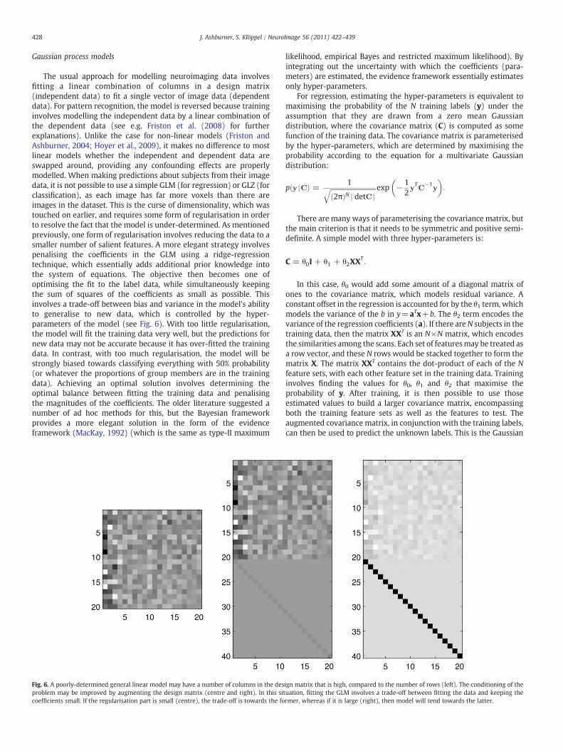
The usual approach for modelling neuroimaging data involvesfitting a linear combination of columns in a design matrix(independent data) to fit a single vector of image data (dependentdata). For pattern recognition, the model is reversed because traininginvolves modelling the independent data by a linear combination ofthe dependent data (see e.g. Friston et al. (2008) for furtherexplanations). Unlike the case for non-linear models (Friston andAshburner, 2004; Hoyer et al., 2009), it makes no difference to mostlinear models whether the independent and dependent data areswapped around, providing any confounding effects are properlymodelled. When making predictions about subjects from their imagedata, it is not possible to use a simple GLM (for regression) or GLZ (forclassification), as each image has far more voxels than there areimages in the dataset. This is the curse of dimensionality, which wastouched on earlier, and requires some form of regularisation in orderto resolve the fact that the model is under-determined. As mentionedpreviously, one form of regularisation involves reducing the data to asmaller number of salient features. A more elegant strategy involvespenalising the coefficients in the GLM using a ridge-regressiontechnique, which essentially adds additional prior knowledge intothe system of equations. The objective then becomes one ofoptimising the fit to the label data, while simultaneously keepingthe sum of squares of the coefficients as small as possible. Thisinvolves a trade-off between bias and variance in the model's abilityto generalise to new data, which is controlled by the hyper-parameters of the model (see Fig. 6). With too little regularisation,the model will fit the training data very well, but the predictions fornew data may not be accurate because it has over-fitted the trainingdata. In contrast, with too much regularisation, the model will bestrongly biased towards classifying everything with 50% probability(or whatever the proportions of group members are in the trainingdata). Achieving an optimal solution involves determining theoptimal balance between fitting the training data and penalisingthe magnitudes of the coefficients. The older literature suggested anumber of ad hoc methods for this, but the Bayesian frameworkprovides a more elegant solution in the form of the evidenceframework (MacKay, 1992) (which is the same as type-II maximum

Fig. 6. A poorly-determined general linear model may have a number of columns in the desproblem may be improved by augmenting the design matrix (centre and right). In this sicoefficients small. If the regularisation part is small (centre), the trade-off is towards the fo

likelihood, empirical Bayes and restricted maximum likelihood). Byintegrating out the uncertainty with which the coefficients (para-meters) are estimated, the evidence framework essentially estimatesonly hyper-parameters.

For regression, estimating the hyper-parameters is equivalent tomaximising the probability of the N training labels (y) under theassumption that they are drawn from a zero mean Gaussiandistribution, where the covariance matrix (C) is computed as somefunction of the training data. The covariance matrix is parameterisedby the hyper-parameters, which are determined by maximising theprobability according to the equation for a multivariate Gaussiandistribution:

p y jCð Þ = 1ffiffiffiffiffiffiffiffiffiffiffiffiffiffiffiffiffiffiffiffiffiffiffiffiffiffiffiffiffi2πð ÞN j detC j

q exp −12yTC

−1y

� �:

There are many ways of parameterising the covariance matrix, butthe main criterion is that it needs to be symmetric and positive semi-definite. A simple model with three hyper-parameters is:

C = θ0I + θ1 + θ2XXT:

In this case, θ0 would add some amount of a diagonal matrix ofones to the covariance matrix, which models residual variance. Aconstant offset in the regression is accounted for by the θ1 term, whichmodels the variance of the b in y=aTx+b. The θ2 term encodes thevariance of the regression coefficients (a). If there are N subjects in thetraining data, then the matrix XXT is an N×N matrix, which encodesthe similarities among the scans. Each set of featuresmay be treated asa row vector, and these N rows would be stacked together to form thematrix X. The matrix XXT contains the dot-product of each of the Nfeature sets, with each other feature set in the training data. Traininginvolves finding the values for θ0, θ1 and θ2 that maximise theprobability of y. After training, it is then possible to use thoseestimated values to build a larger covariance matrix, encompassingboth the training feature sets as well as the features to test. Theaugmented covariance matrix, in conjunction with the training labels,can then be used to predict the unknown labels. This is the Gaussian

ign matrix that is high, compared to the number of rows (left). The conditioning of thetuation, fitting the GLM involves a trade-off between fitting the data and keeping thermer, whereas if it is large (right), then model will tend towards the latter.

429J. Ashburner, S. Klöppel / NeuroImage 56 (2011) 422–439

process regression framework (Williams and Rasmussen, 1996), andis nicely described in textbooks such as MacKay (2003),4 Rasmussenand Williams (2006)5 or Bishop et al. (2006). There is also a relatedframework for classification (Williams and Barber, 1998), althoughpractical implementation is not so straightforward, and often involvesa number of approximations.6 The important point here, is thatGaussian process classification also requires a covariance matrix,which is formulated in the same way as that for regression.

Feature selectionIf some features of the data are known to be less informative than

others, then it is possible to down-weight their importance. Similarly,if it is known, a priori, that a sparse set of features are likely toprovide the most accurate predictions, then the pattern recognitionalgorithm may be modified such that it is more likely to select asparse set of features. A number of authors have devised featureselection procedures for applying pattern recognition to imagingdata. The objective of feature selection is to ignore, or down-weight,those features that provide relatively less discriminatory signal.Within the Gaussian process framework, this would be analogous toignoring the contribution made, by those features, to the matrix ofdot-products.

This kind of naïve feature selection may be formulated using adiagonal matrix, W, which is a function of several, non-negative,hyper-parameters (θ2, θ3, etc). The limiting case of this frameworkwould be the situation where each element on the diagonal of W wasone of the hyper-parameters. This is known as automatic relevancedetermination, and usually results in sparse solutions as some of thehyper-parameters fall to zero. Solutions obtained from this model areequivalent to those described in Friston et al. (2008). For this kind ofmodel, the covariance matrix would be given by:

C = θ0I + θ1 + XW θ2; θ3…ð ÞXT: ð1Þ

Sparsity may be over space, but this need not be the case. It ispossible that pre-processing models, such as independent componentanalysis (Bell and Sejnowski, 1995), could transform the data into thekind of features whereby selecting a sparse subset would addbiological plausibility to the discrimination. Similarly, there areother factorisation models that could prove useful for defining thekinds of features where sparsity would be advantageous. One suchexample may be non-negative matrix factorisation (Lee and Seung,1999).

There is no reason why W should be limited to the diagonal case.For example, if the features consist of image data that have been pre-processed in some way, then W could encode a convolution function,such that the algorithm may determine the optimal degree of spatialblurring. It is often the case that low spatial frequencies containproportionally more informative signal than do the higher frequen-cies, so more accurate predictions may be obtained by blurring thedata by some optimal amount.

Later, the paper will explain a possible framework for this type ofapproach, whereby a similar Wmatrix may be used to obtain a trade-off between information pertaining to shape, and informationpertaining to image intensity.

Going non-linearSometimes, it is not possible to achieve accurate predictions using

a linear separation method, in which case non-linear methods may berequired. For example, a particular disorder may be characterised by a

4 This book is freely available at http://www.inference.phy.cam.ac.uk/mackay/itila/.5 This book is freely available at http://www.gaussianprocess.org/gpml/chapters/.6 See http://www.gaussianprocess.org/ for some implementations, and other useful

information.

number of alternative types of variability. A simple example would bea disorder that either causes atrophy in the left or in the righthemisphere. A linear model would only be able to encode onemode ofvariability, whereas a non-linear model may be able to capture bothmodes.

Non-linear models work by projecting the data into a highernumber of dimensions, where they can be fitted using a linear model(see e.g., Cristianini and Shawe-Taylor (2000), Bishop et al. (2006)).This is similar to the use of polynomial expansions for simple non-linear fitting of data. There is a class of methods, known as kernelmethods, that is ideally suited to this approach. These methods use thekernel trick, which involves replacing the matrix of dot-products(XXT) by some other symmetric and positive semi-definite matrix,which is a function of the data. One of the most widely used forms forthis matrix is one based on radial basis functions (RBF), whichrequires distances between all pairs of feature vectors. It is possible toderive distances from matrices of dot-products because (x1−x2)2=x12+x2

2−2x1x2. Each element of the matrix would then be replaced byexp −θ

2d2mn

� �, where d is the distance between feature set m and

feature set n, and θ is a hyper-parameter controlling the width of thekernel.

Rather than use simple Euclidean distances between each pair offeature sets, it is also possible to use othermeasures of distancewithinthe RBF framework. The only requirement is that the measures mustsatisfy the requirements for being a metric, which are:

1. They must be greater than or equal to zero.2. They may only be equal to zero if the features are identical.3. The distance between xm and xn must be equal to the distance

between xn and xm.4. The distance between xm and xn must not be greater than the sum

of those between xm and xk, and between xk and xn.

A strategy for deriving metrics between shapes will be describedlater. Many pattern recognition procedures can be formulated askernel methods, but several other algorithms can also be kernelised.

Non-linear methods allow more complicated separations to beachieved, but they also make it easier for the model to over-fit thetraining data. As in the case of the previous examples, the hyper-parameter(s) controlling the degree of non-linearity may be auto-matically determined using the evidence framework. Also, interpret-ing the mechanism by which separation is achieved is much moredifficult when non-linear methods are used (Golland, 2002). Ideally,linear methods would be used whenever possible, but this mayrequire representing the features in a form that allows easierseparation using a linear method.

Real data often falls in manifold-like patterns within the high-dimensional space (see e.g. Baloch and Davatzikos (2009)), but thecareful use of generative models may allow much of this pattern to bemodelled. A simple example would be an image of a brain that isrigidly transformed by various amounts. There are six parameterscontrolling the rigid transform, so the transformed versions of theimage would fall as points on a six-dimensional manifold. Rigid-bodyalignment could be used to bring all the points on themanifold back toa single point. Similarly, inter-subject registration methods are able tomodel out some of the manifold-like patterns within MRI data. Unlikethe rigid-body alignment case, the way that the spatial transformationis encoded is also of interest because it describes the shape of thebrain. To be as powerful as possible, pattern recognition for studies ofinter-subject variability should be formulated to work both withshape descriptors, and also with the variability that cannot bemodelled out by alignment.

Measuring empirical success

Many classification methods are able to fully separate the trainingdata, whereas they may generalise poorly to novel data. Often, cross-

430 J. Ashburner, S. Klöppel / NeuroImage 56 (2011) 422–439

validation is used to assess how accurately the characterisationseparates the populations.7 This may involve fitting the model to allsubjects' data except for one, and then assessing the accuracy of theprediction about the subject that was left out. The procedurewould berepeated by leaving out the next subject's data, and so on. Reports ofsensitivity and specificity, using measures such as the area under thereceiver operating characteristic (ROC) curve (see e.g. Zou et al.(2007)), can be compared with those of human experts. Humanexpertise is still considered to be the gold standard to beat for mostmodels encoding image understanding (Kloppel et al., 2008a). Thissituation may change over the next few years, as computing powerwill probably continue to grow exponentially (“Moore's Law”), thusallowing new levels of algorithmic sophistication.

In other situations, the comparisons tend to be among computermodels, and cross-validation is less likely to be used. Measures, suchas the Bayesian model evidence, minimum description length (MDL),Bayesian information criterion (BIC) and the Akaike informationcriterion (AIC), may be used for assessing how well models encodeprobability densities, thus allowing the evidence for different modelsto be compared, so that the best model for each particular datasetmay be selected. Real Bayesian modellers do not use cross-validation,and the neuroimaging field is seeing the increasing use of evidencemeasures for choosing among models (Penny et al., 2004; Beckmannand Smith, 2004; Friston et al., 2007; Behrens et al., 2007; Fristonet al., 2008; Kiebel et al., 2008). Providing all the model assumptionsare met, Bayesian strategies for model selection are more efficient –both in terms of computational complexity, and in terms of theavailable degrees of freedom (Rasmussen and Williams, 2006) – thancross-validation for selecting the optimal model from a number ofcandidates.

Cross-validation is often used for optimising feature selection, orfor adjusting other settings in the model. If there are not too manysettings to adjust, then a grid search strategy can be used, where arange of settings are tried, and the most successful is chosen.However, within the Bayesian modelling framework, this type ofapproach can be greatly streamlined. The best model is the one withthe highest model evidence, and the model fitting procedures aregeared towards searching over the space of possible hyper-para-meters in order to maximise this measure.

Large datasets

Some investigators object to the Bayesian view of modellingbecause it involves the use of prior knowledge. Other approaches,such as orthodox statistical techniques, also involve some form ofsubjectivity — but this subjectivity is usually hidden. For example,what is so special about a value of 0.05 when assessing thesignificance of a p value? Should a correction formultiple comparisonsbe used when interpreting findings from multiple studies? ForBayesian methods, the relative effect of the priors becomes lessimportant for large datasets, so findings become less subjective asmore data are modelled.

Bayesian model selection strategies try to identify the mostappropriate model for the data, and the optimal choice relates tothe quantity and quality of data. As more becomes available, thecomplexity of the optimal model will continue to increase until itreaches that of the system under study. In the case of biologicalsystems, this complexity is likely to exceed that of typical datasets. Forthis reason (and others), the sharing and re-utilisation of valuable andwell characterised data is likely to become increasingly important forthe integrative models that are required for research in both systemsbiology and for translational work (Van Horn and Toga, 2009).

7 Cross-validation is exactly analogous to the hypothesis testing approach that iscommonly accepted within the field, except that the hypotheses have been learned bya pattern recognition algorithm.

Relatively few investigators build on primary data from previous fMRIstudies because of the subjectivity of the stimuli used, and thedifficulties inherent in attempting to organise the experiments intoany useful structure. In contrast, as demonstrated by ADNI (Muelleret al., 2005; Butcher, 2007) and other similar projects (Marcus et al.,2007), the primary data required for studies of anatomical variabilitytend to be re-used and built on extensively. Just as data generated bythe Human Genome Project would be relatively worthless if only oneinvestigator had access to it, the same may be true of primary datafrom large studies of neuroanatomical variability. If data is ofsufficiently high quality and relevant, then others will wish to use it.Measures such as the h-index are becoming increasingly important asmeasures of productivity (rather than simply the numbers ofpublications) (Hirsch, 2007). Not only would data-sharing increasetransparency and reproducibility of the scientific process, but it is alsoa way to helpmaximise the impact of work. Many funding bodies nowrequire some sharing of primary data, and terms such as “mega-analysis” are beginning to enter the vocabularies of neuroimagers(Salimi-Khorshidi et al., 2009). Inevitably, some researchers willobject to mixing data from different scanners, sequences etc, claimingthat models of data collected on one scanner cannot be generalised todata from another. This is not an argument against pooling data, but isinstead a quite different one.

Given the exponentially increasing ease with which genes can besequenced (and the exponentially decreasing cost), sharing primarydata is likely to become especially important for future studiesattempting to link genotype with phenotype. A search throughhundreds of thousands, or even millions, of single nucleotidepolymorphisms (or – within a few years – entire genomes) presentsa colossal multiple comparisons problem. For this type of work, theaim would be to find those alleles that have the greatest measurableeffect (any effect) on brain anatomy (or function). Identifying thosegenetic associations that best predict neuroanatomical variability willrequire multivariate modelling of very large datasets. Anotherapproach to finding further clues about the causes of various disorderswould be to generate a multivariate characterisation of the typicalpattern of deviation from a control population. This pattern may beexpressed to various degrees in the healthy population, which leads tothe possibility of probing for the pattern in a large population ofgenetically characterised subjects.8

Generative modelling

Data are usually pre-processed by modelling them generatively inorder to derive useful features, which are subsequently fed into thediscriminative framework. This section deals with certain aspects ofPattern Theory, which is a generative modelling framework thatbegins with the premise that real world patterns are complex, andthat encoding this complexity should be allowed (Mumford, 1996;Mumford, 2002; Grenander and Miller, 2007). Simplifying organisa-tional principles may emerge from such complex models, but thesewould not be discovered unless the data is modelled in all itscomplexity. Currently, much of Pattern Theory concerns shapemodelling, although it is an area of research that is likely to expandand subsume a wider variety of probabilistic models. In principle,Pattern Theory is not really so different from other reputableBayesian modelling strategies, but its ambitions may be greater inthat it was formulated to deal with the kind of complexityencountered in biological systems. The ideas proposed within thisreview differ from the Pattern Theory perspective in that thegenerative modelling is treated as a pre-curser to a discriminativemodelling step. Pattern Theory would involve a single unifyinggenerative model for everything.

8 Geoffrey Tan, personal communication.

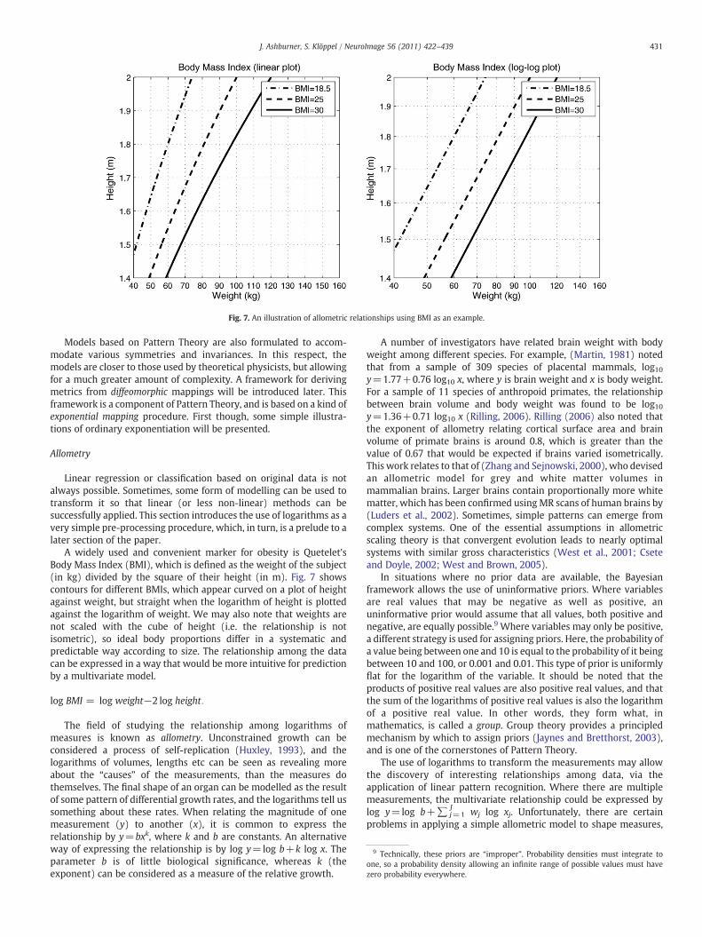
Fig. 7. An illustration of allometric relationships using BMI as an example.

9 Technically, these priors are “improper”. Probability densities must integrate toone, so a probability density allowing an infinite range of possible values must havezero probability everywhere.

431J. Ashburner, S. Klöppel / NeuroImage 56 (2011) 422–439

Models based on Pattern Theory are also formulated to accom-modate various symmetries and invariances. In this respect, themodels are closer to those used by theoretical physicists, but allowingfor a much greater amount of complexity. A framework for derivingmetrics from diffeomorphic mappings will be introduced later. Thisframework is a component of Pattern Theory, and is based on a kind ofexponential mapping procedure. First though, some simple illustra-tions of ordinary exponentiation will be presented.

Allometry

Linear regression or classification based on original data is notalways possible. Sometimes, some form of modelling can be used totransform it so that linear (or less non-linear) methods can besuccessfully applied. This section introduces the use of logarithms as avery simple pre-processing procedure, which, in turn, is a prelude to alater section of the paper.

A widely used and convenient marker for obesity is Quetelet'sBody Mass Index (BMI), which is defined as the weight of the subject(in kg) divided by the square of their height (in m). Fig. 7 showscontours for different BMIs, which appear curved on a plot of heightagainst weight, but straight when the logarithm of height is plottedagainst the logarithm of weight. We may also note that weights arenot scaled with the cube of height (i.e. the relationship is notisometric), so ideal body proportions differ in a systematic andpredictable way according to size. The relationship among the datacan be expressed in a way that would be more intuitive for predictionby a multivariate model.

log BMI = log weight−2 log height:

The field of studying the relationship among logarithms ofmeasures is known as allometry. Unconstrained growth can beconsidered a process of self-replication (Huxley, 1993), and thelogarithms of volumes, lengths etc can be seen as revealing moreabout the “causes” of the measurements, than the measures dothemselves. The final shape of an organ can be modelled as the resultof some pattern of differential growth rates, and the logarithms tell ussomething about these rates. When relating the magnitude of onemeasurement (y) to another (x), it is common to express therelationship by y=bxk, where k and b are constants. An alternativeway of expressing the relationship is by log y=log b+k log x. Theparameter b is of little biological significance, whereas k (theexponent) can be considered as a measure of the relative growth.

A number of investigators have related brain weight with bodyweight among different species. For example, (Martin, 1981) notedthat from a sample of 309 species of placental mammals, log10y=1.77+0.76 log10 x, where y is brain weight and x is body weight.For a sample of 11 species of anthropoid primates, the relationshipbetween brain volume and body weight was found to be log10y=1.36+0.71 log10 x (Rilling, 2006). Rilling (2006) also noted thatthe exponent of allometry relating cortical surface area and brainvolume of primate brains is around 0.8, which is greater than thevalue of 0.67 that would be expected if brains varied isometrically.This work relates to that of (Zhang and Sejnowski, 2000), who devisedan allometric model for grey and white matter volumes inmammalian brains. Larger brains contain proportionally more whitematter, which has been confirmed using MR scans of human brains by(Luders et al., 2002). Sometimes, simple patterns can emerge fromcomplex systems. One of the essential assumptions in allometricscaling theory is that convergent evolution leads to nearly optimalsystems with similar gross characteristics (West et al., 2001; Cseteand Doyle, 2002; West and Brown, 2005).

In situations where no prior data are available, the Bayesianframework allows the use of uninformative priors. Where variablesare real values that may be negative as well as positive, anuninformative prior would assume that all values, both positive andnegative, are equally possible.9 Where variables may only be positive,a different strategy is used for assigning priors. Here, the probability ofa value being between one and 10 is equal to the probability of it beingbetween 10 and 100, or 0.001 and 0.01. This type of prior is uniformlyflat for the logarithm of the variable. It should be noted that theproducts of positive real values are also positive real values, and thatthe sum of the logarithms of positive real values is also the logarithmof a positive real value. In other words, they form what, inmathematics, is called a group. Group theory provides a principledmechanism by which to assign priors (Jaynes and Bretthorst, 2003),and is one of the cornerstones of Pattern Theory.

The use of logarithms to transform the measurements may allowthe discovery of interesting relationships among data, via theapplication of linear pattern recognition. Where there are multiplemeasurements, the multivariate relationship could be expressed bylog y=log b+∑ j=1

Jwj log xj. Unfortunately, there are certain

problems in applying a simple allometric model to shape measures,

432 J. Ashburner, S. Klöppel / NeuroImage 56 (2011) 422–439

which occur because growth is not unconstrained, and neighbouringor overlapping structures need to grow together. Huxley (1993)pointed out that the logarithm of the volume/mass of a structureshould be related to the volume/mass of the whole organism minusthat of the structure. Similar concerns were identified by (Zhang andSejnowski, 2000), who related grey matter volume to white mattervolume, and also grey matter volume to the sum of grey and whitematter volume. If the relationship that log y=log b+k log x holds,then it is not possible for log y=log b′+k′log(x+y) also to hold.Resolving this inconsistency requires a different model to account forsuch correlations. That model may be the one based on the group ofdiffeomorphisms.

Identical functions of very different coordinate systems

Merriam-Webster's Medical Dictionary defines morphometry asthe quantitative measurement of the form especially of living systemsor their parts, where form means the shape and structure ofsomething as distinguished from its material. The study of form islargely derived from the generative model of D'Arcy Thompson(Thompson and Bonner, 1942), who stated that ‘diverse anddissimilar fish [brains] can be referred as a whole to identicalfunctions of very different coordinate systems, this fact will of itselfconstitute a proof that a comprehensive “law of growth” has pervadedthe whole structure in its integrity, and that some more or less simpleand recognizable system of forces has been at work’.

Conventionally, the neuroimaging field treats inter-subject vari-ability as different functions of near-identical coordinate systems.fMRI studies, involving comparisons among populations of subjects,usually attribute their findings to what may be referred to as“functional variability”, whereas many of the results could equallybe attributable to variability of the underlying anatomy. Interpreta-tions of exactly what is meant by functional variability may includevariability of the magnitude of activations, or activations occurringwithin non-homologous structures. Unfortunately, the very definitionof what constitutes a homology is unclear, which makes it difficult todraw any sharp distinction between “functional” and “anatomical”variability.

Literal adherence to Thompson's model would have implicationsfor how functional data should be used to further our understandingof inter-subject variability. Such a model would require that fMRI beused as a way of labeling the various regions of functionalspecialization, thereby allowing image registration procedures tobring these labeled regions into alignment (Saxe et al., 2006; Sabuncuet al., 2009). Studies of inter-subject variability could then be basedupon the relative shapes of the brains, as estimated by registrationalgorithms.

Similarly, diffusion weighted MRI could provide information thatallows more accurate measurement of relative shape (Behrens et al.,2003, 2006; Klein et al., 2007; Johansen-Berg et al., 2005). Under anassumption that brains all have the same pattern of major tracts, itwould appear reasonable to align the brains based on their tracts andsimply compare the resulting shapes. A number of approaches arealready being developed to align brains using diffusion data(Alexander et al., 1999; Guimond et al., 2002; Ruiz-Alzola, 2002;Park et al., 2003; Zhang et al., 2006). It is common for investigators towant to compare the positions of tracts among spatially normalisedimages, but findings from such an analysis would essentially be aboutmis-registration. This is useful for evaluating image registrationmodels, but would not necessarily be considered interesting from aphysiological perspective.

In reality, the pure D'Arcy Thompson model may over-exaggeratethe importance of form to our understanding of variability. Languagelateralization provides a clear example of where such a model wouldfail, as it involves patterns of functional specialization that couldclearly not be modelled by shape differences alone. Because the term

“homologous” is only vaguely defined, future advances to ourunderstanding of variability may be more likely to arise from modelsthat have the potential to combine form-like and function-likevariance, in an elegant and parsimonious manner.

Shapemodels are an important component of the feature sets usedfor pattern recognition (Golland et al., 2001, 2005), but features basedon residual differences after registration are also of potentialimportance (Makrogiannis et al., 2007), particularly if informationfrom fMRI or diffusion imaging is to be included within themodel. It ispossible that increased power may be achieved by using a moresophisticated model for these patterns of residual variability (Trouvéand Younes, 2005). There is much that could be said on the subject oftemplatemodels of the brain and how they relate to this pattern, but itwould be beyond the scope of this review. In the next sections, wewilltry to explain how the residual differences after registration canactually be used to encode deformations (Younes, 2007). Theregistration model that is needed for achieving this goal appearsrather more complicated than most, but it may have the potential tosimplify the feature sets used for multivariate analysis.

Diffeomorphic shape models

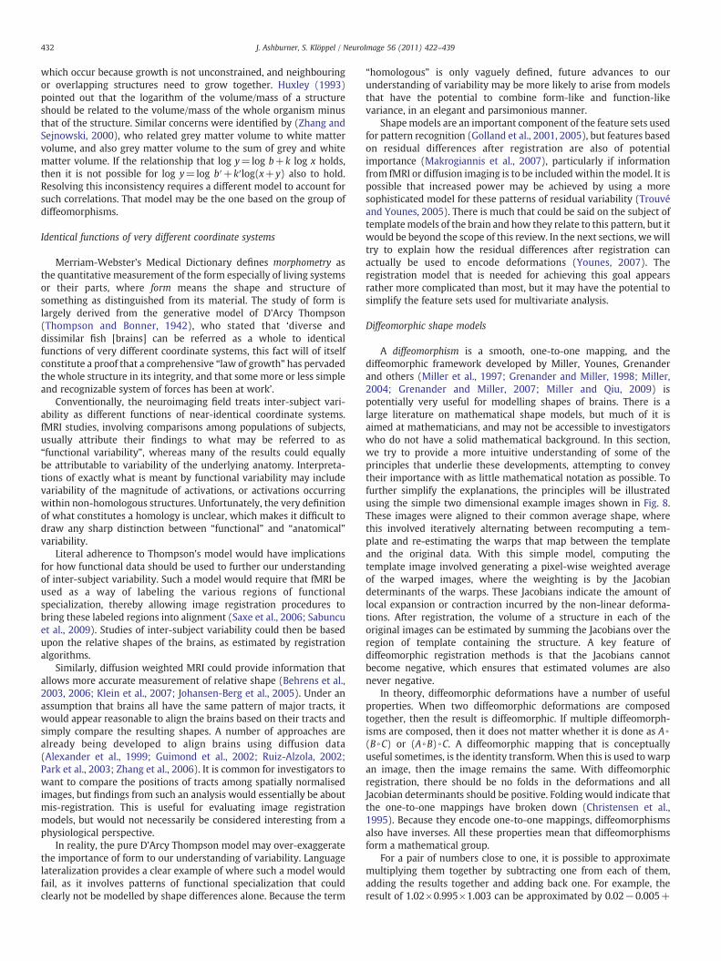
A diffeomorphism is a smooth, one-to-one mapping, and thediffeomorphic framework developed by Miller, Younes, Grenanderand others (Miller et al., 1997; Grenander and Miller, 1998; Miller,2004; Grenander and Miller, 2007; Miller and Qiu, 2009) ispotentially very useful for modelling shapes of brains. There is alarge literature on mathematical shape models, but much of it isaimed at mathematicians, and may not be accessible to investigatorswho do not have a solid mathematical background. In this section,we try to provide a more intuitive understanding of some of theprinciples that underlie these developments, attempting to conveytheir importance with as little mathematical notation as possible. Tofurther simplify the explanations, the principles will be illustratedusing the simple two dimensional example images shown in Fig. 8.These images were aligned to their common average shape, wherethis involved iteratively alternating between recomputing a tem-plate and re-estimating the warps that map between the templateand the original data. With this simple model, computing thetemplate image involved generating a pixel-wise weighted averageof the warped images, where the weighting is by the Jacobiandeterminants of the warps. These Jacobians indicate the amount oflocal expansion or contraction incurred by the non-linear deforma-tions. After registration, the volume of a structure in each of theoriginal images can be estimated by summing the Jacobians over theregion of template containing the structure. A key feature ofdiffeomorphic registration methods is that the Jacobians cannotbecome negative, which ensures that estimated volumes are alsonever negative.

In theory, diffeomorphic deformations have a number of usefulproperties. When two diffeomorphic deformations are composedtogether, then the result is diffeomorphic. If multiple diffeomorph-isms are composed, then it does not matter whether it is done as A ∘(B ∘C) or (A ∘B) ∘C. A diffeomorphic mapping that is conceptuallyuseful sometimes, is the identity transform.When this is used to warpan image, then the image remains the same. With diffeomorphicregistration, there should be no folds in the deformations and allJacobian determinants should be positive. Folding would indicate thatthe one-to-one mappings have broken down (Christensen et al.,1995). Because they encode one-to-one mappings, diffeomorphismsalso have inverses. All these properties mean that diffeomorphismsform a mathematical group.

For a pair of numbers close to one, it is possible to approximatemultiplying them together by subtracting one from each of them,adding the results together and adding back one. For example, theresult of 1.02×0.995×1.003 can be approximated by 0.02−0.005+

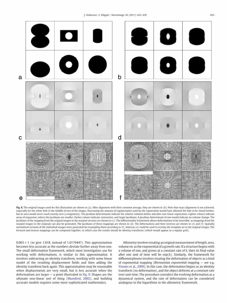
Fig. 8. The original images used for this illustration are shown in (a). After alignment with their common average, they are shown in (b). Note that exact alignment is not achieved,especially for the white hole in the middle of two of the images. Decreasing the amount of regularisation used by the registration would have allowed the hole to be closed further,but its area would never reach exactly zero (a singularity). The Jacobian determinants indicate the relative volumes before and after non-linear registration. Lighter colours indicateareas of expansion, where the Jacobians are smaller. Darker colours indicate contraction, and larger Jacobians. A Jacobian determinant of one would indicate no volume change. TheJacobians of themapping from the original images to thewarped versions are shown in (c). The diffeomorphic framework allows deformations to be invertible, somappings from thewarped images to the originals can also be generated. The Jacobians of these mappings are shown in (d). The deformations and their inverses are shown in (e) and (f). Spatiallynormalised versions of the individual images were generated by resampling them according to (f), whereas (e) could be used to overlay the template on to the original images. Theforward and inverse mappings can be composed together, in which case the results should be identity transforms (which would appear as a regular grid).

433J. Ashburner, S. Klöppel / NeuroImage 56 (2011) 422–439

0.003+1 (to give 1.018, instead of 1.0179447). This approximationbecomes less accurate as the numbers deviate further away from one.The small deformation framework, which most investigators use forworking with deformations, is similar to this approximation. Itinvolves subtracting an identity transform, working with some linearmodel of the resulting displacement fields and then adding theidentity transform back again. This approximation may be reasonablewhen displacements are very small, but is less accurate when thedeformations are larger — a point illustrated in Fig. 9. Shapes are theultimate non-linear sort of thing (Mumford, 2002), and buildingaccurate models requires some more sophisticated mathematics.

Allometry involves treating anoriginalmeasurement of length, area,volumeetc as the exponential of a growth rate. If a structure beginswitha volume of one, and grows at a constant rate of k, then its final valueafter one unit of time will be exp(k). Similarly, the framework fordiffeomorphisms involves treating the deformation of objects as a kindof exponential mapping (Riemannian exponential mapping — see e.g.Younes et al., 2009). In this case, the deformation begins as an identitytransform (no deformation), and the object deforms at a constant rateover unit time. The procedure considers the evolving deformation as adynamical system, and the rate of deformation can be consideredanalogous to the logarithms in the allometric framework.

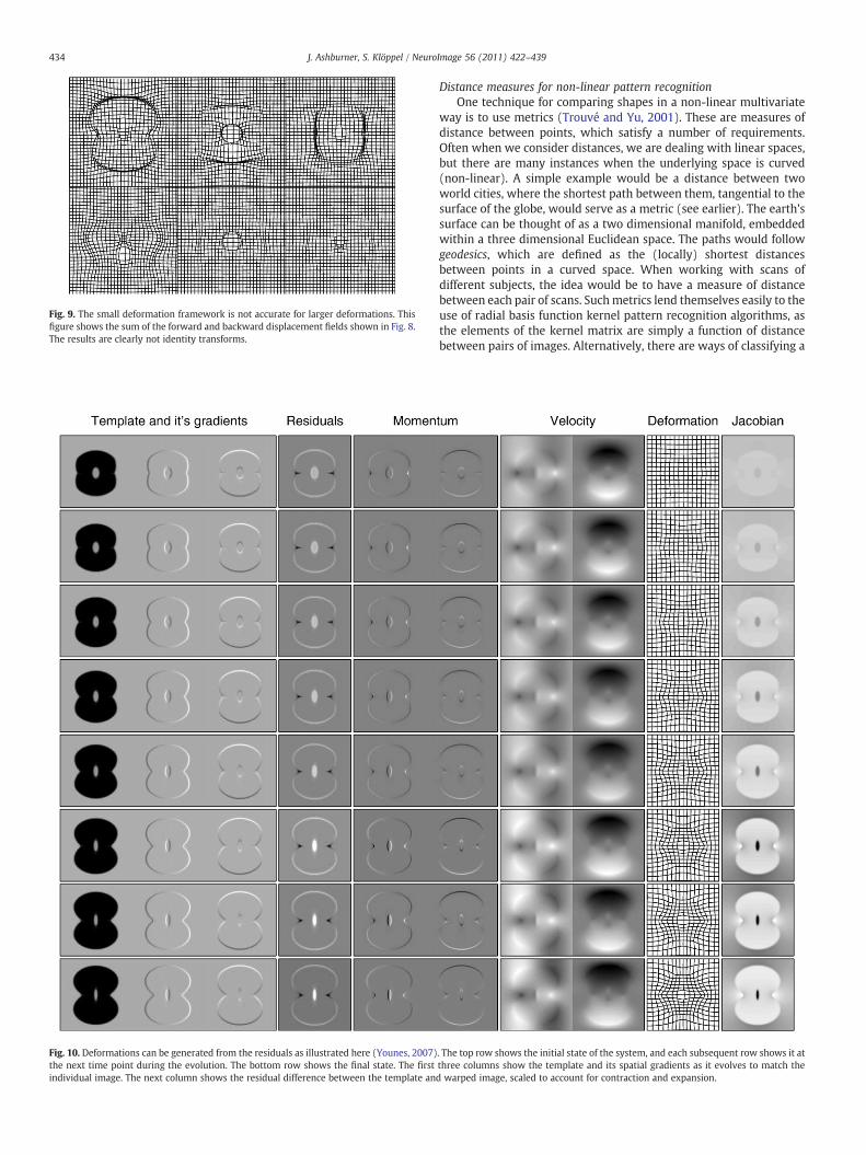
Fig. 9. The small deformation framework is not accurate for larger deformations. Thisfigure shows the sum of the forward and backward displacement fields shown in Fig. 8.The results are clearly not identity transforms.

Fig. 10. Deformations can be generated from the residuals as illustrated here (Younes, 2007)the next time point during the evolution. The bottom row shows the final state. The firstindividual image. The next column shows the residual difference between the template an

434 J. Ashburner, S. Klöppel / NeuroImage 56 (2011) 422–439

Distance measures for non-linear pattern recognitionOne technique for comparing shapes in a non-linear multivariate

way is to use metrics (Trouvé and Yu, 2001). These are measures ofdistance between points, which satisfy a number of requirements.Often when we consider distances, we are dealing with linear spaces,but there are many instances when the underlying space is curved(non-linear). A simple example would be a distance between twoworld cities, where the shortest path between them, tangential to thesurface of the globe, would serve as a metric (see earlier). The earth'ssurface can be thought of as a two dimensional manifold, embeddedwithin a three dimensional Euclidean space. The paths would followgeodesics, which are defined as the (locally) shortest distancesbetween points in a curved space. When working with scans ofdifferent subjects, the idea would be to have a measure of distancebetween each pair of scans. Suchmetrics lend themselves easily to theuse of radial basis function kernel pattern recognition algorithms, asthe elements of the kernel matrix are simply a function of distancebetween pairs of images. Alternatively, there are ways of classifying a

. The top row shows the initial state of the system, and each subsequent row shows it atthree columns show the template and its spatial gradients as it evolves to match thed warped image, scaled to account for contraction and expansion.

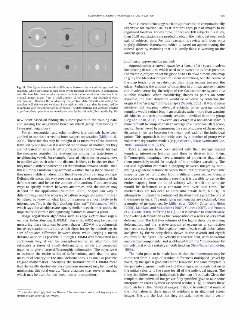
Fig. 11. This figure shows residual differences between the warped images and thetemplate, which are scaled at each point by the Jacobian determinant. In conjunctionwith the template, these residuals encode the information needed to reconstruct theoriginal images (apart from a small amount of information lost through inexactinterpolation). Dividing the residuals by the Jacobian determinants and adding thetemplate will give warped versions of the originals, which can then be unwarped byresampling with the appropriate deformation. The deformations and Jacobians neededto perform these operations are actually encoded by the residuals (illustrated in Fig. 10).

435J. Ashburner, S. Klöppel / NeuroImage 56 (2011) 422–439

new point based on finding the closest points in the training data,and making the assignment based on which group they belong to(K-nearest neighbour).

Pattern recognition and other multivariate methods have beenapplied to metrics derived by inter-subject registration (Miller et al.,2008). These metrics may be thought of as measures of the distancetravelled by one brain as it is warped to the shape of another, but theyare not based on simple lengths of trajectories of the voxels. Instead,the measures consider the relationships among the trajectories ofneighbouring voxels. For example, if a set of neighbouring voxelsmovein parallel with each other, the distance is likely to be shorter than iftheymove in different directions. If theirmotion remains parallel, thenthis is simply a uniform displacement— rather than a shape change. Iftheymove in different directions, then this results in a change of shape.Defining distances this way provides a measure of smoothness of thedeformations, and hence the amount of distortion. There are manyways to specify metrics between anatomies, and the choice maydepend on the application (Mumford, 2005). Shapes can vary indifferent ways, and the accuracy of pattern recognition algorithms canbe helped by knowing what kind of measures are most likely to beinformative. This is the Ugly Duckling Theorem10 (Watanabe, 1969),which says that all objects are equally similar to each other, unless theimportance of certain distinguishing features is known a priori.

Image registration algorithms such as Large Deformation Diffeo-morphic Metric Mapping (LDDMM) (Beg et al., 2005) may be used formeasuring these distances between shapes. LDDMM is a volumetricimage registration procedure, which aligns images by minimising thesum of squares difference between them, while keeping a metricdistance as short as possible. Although LDDMM was formulated in acontinuous way, it can be conceptualised as an algorithm thatestimates a series of small deformations, which are composedtogether to give a large diffeomorphic deformation. The objective isto estimate the entire series of deformations, such that the totalmeasure of “energy” in the small deformations is as small as possible.Elegant mathematics underlying the formulation of LDDMM meanthat the locally shortest distance (geodesic distance) may be found byminimising this total energy. These distances may serve as metrics,which may be used for non-linear pattern recognition.

10 It is called the “Ugly Duckling Theorem” because a swan and a duckling are just assimilar to each other as two swans.

With current technology, such an approach is too computationallyexpensive for routine use, as it requires each pair of images to beregistered together. For example, if there are 100 subjects in a study,then 5050 registrations are needed to obtain the metric between eachpair of subjects' data. For this reason, this review will focus on aslightly different framework, which is based on approximating thecurved space by assuming that it is locally flat (i.e. working on thetangent space).

Local linear approximation methodsApproximating a curved space by a linear (flat) space involves

introducing distortions, which need to be overcome as far as possible.For example, projections of the globe on to a flat two dimensional map(e.g. by the Mercator projection) incur distortions, but the centre ofthe map tends to be less distorted than those regions towards theedges. Reducing the amount of distortion in a linear approximationcan involve centering the origin of the flat coordinate system at asuitable location. When considering shapes as points on somemanifold, the least distortion would be achieved by centering theorigin at the “average” of those shapes (Woods, 2003). It would seemintuitive that warping individual subjects to an average shapedtemplate would reduce bias in an analysis, rather more than warpingall subjects to match a randomly selected individual from the group(Beg and Khan, 2006). However, an average in a non-linear space ismore difficult to compute than an average in a Euclidean (flat) space,and can be achieved by minimising the sum of squares of the geodesicdistances (metrics) between the mean, and each of the individualpoints. This approach is implicitly used by a number of group-wisevolumetric registration models (e.g. Joshi et al., 2004; Avants and Gee,2004; Lorenzen et al., 2005).

Once all images have been aligned with their average shapedtemplate, interesting features may then be derived from them.Diffeomorphic mappings have a number of properties that makesthem potentially useful for analysis of inter-subject variability. TheLDDMM algorithm estimates a mapping between images by mini-mising a geodesic distance between them, but estimating the samemapping can be formulated from a different perspective. Using aprocedure is known as geodesic shooting, it is possible to derive theentire mapping from the initial velocity with which the templatewould be deformed at a constant rate over unit time. Themathematics are too deep to enter into details here, but Fig. 10attempts to illustrate the evolution of the dynamical system for one ofthe images in Fig. 8. The underlying mathematics are explained, froma number of perspectives, by Miller et al. (2006), Cotter and Holm(2006), Marsland and McLachlan (2007), Younes (2007), and Youneset al. (2008, 2009). Referring to Fig. 10, it is possible to conceptualisethe evolving deformation as the composition of a series of very smalldeformations. The last two columns of the figure show the evolvingdeformation, and the relative amount of expansion or contractionincurred at each point. The displacements of each small deformationare given by the velocity fields shown in the seventh and eighthcolumns of the figure. The velocity is a vector field, with horizontaland vertical components, and is obtained from the “momentum” byconvolving it with a suitably smooth function (Bro-Nielsen and Cotin,1996).

The main point to be made here, is that the momentum may becomputed from a map of residual differences multiplied (voxel byvoxel) by the spatial gradients of the template. The same template iswarped into alignment with each of the images, so its contribution tothe initial velocity is the same for all of the individual images. Thething that differs among individuals is the map of residuals. Given thetemplate, the individual images are fully specified (give or take someinterpolation error) by their associated residuals. Fig. 11 shows theseresiduals for all the individual images. It should be noted that much ofthe information in these maps of residuals is in alignment acrossimages. This and the fact that they are scalar rather than a vector

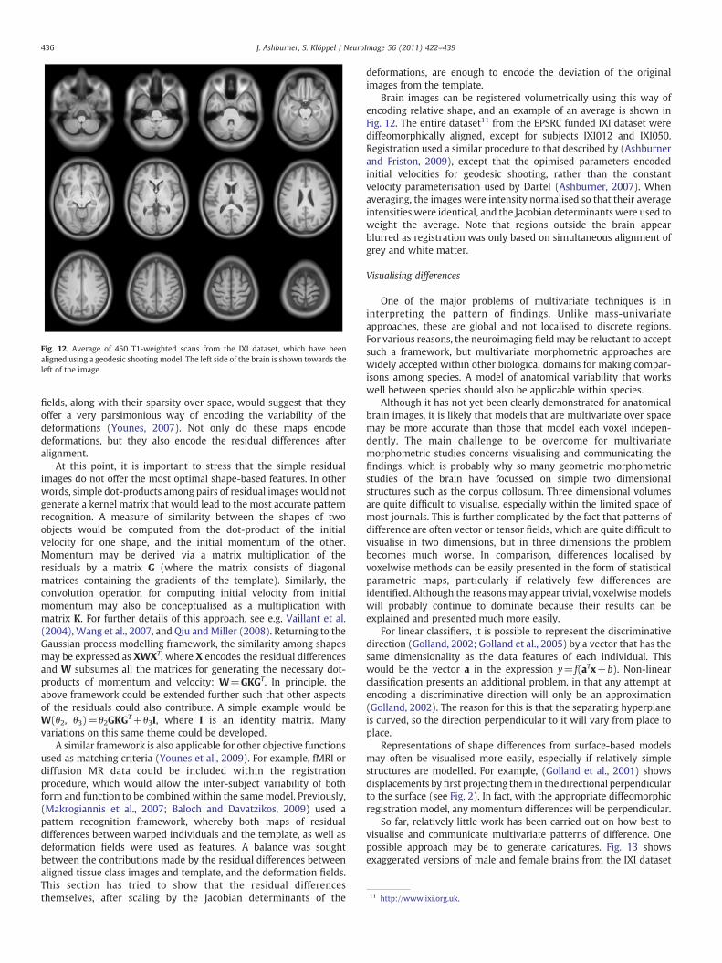
Fig. 12. Average of 450 T1-weighted scans from the IXI dataset, which have beenaligned using a geodesic shooting model. The left side of the brain is shown towards theleft of the image.

11 http://www.ixi.org.uk.

436 J. Ashburner, S. Klöppel / NeuroImage 56 (2011) 422–439

fields, along with their sparsity over space, would suggest that theyoffer a very parsimonious way of encoding the variability of thedeformations (Younes, 2007). Not only do these maps encodedeformations, but they also encode the residual differences afteralignment.

At this point, it is important to stress that the simple residualimages do not offer the most optimal shape-based features. In otherwords, simple dot-products among pairs of residual images would notgenerate a kernel matrix that would lead to the most accurate patternrecognition. A measure of similarity between the shapes of twoobjects would be computed from the dot-product of the initialvelocity for one shape, and the initial momentum of the other.Momentum may be derived via a matrix multiplication of theresiduals by a matrix G (where the matrix consists of diagonalmatrices containing the gradients of the template). Similarly, theconvolution operation for computing initial velocity from initialmomentum may also be conceptualised as a multiplication withmatrix K. For further details of this approach, see e.g. Vaillant et al.(2004), Wang et al., 2007, and Qiu andMiller (2008). Returning to theGaussian process modelling framework, the similarity among shapesmay be expressed as XWXT, where X encodes the residual differencesand W subsumes all the matrices for generating the necessary dot-products of momentum and velocity: W=GKGT. In principle, theabove framework could be extended further such that other aspectsof the residuals could also contribute. A simple example would beW(θ2, θ3)=θ2GKGT+θ3I, where I is an identity matrix. Manyvariations on this same theme could be developed.

A similar framework is also applicable for other objective functionsused as matching criteria (Younes et al., 2009). For example, fMRI ordiffusion MR data could be included within the registrationprocedure, which would allow the inter-subject variability of bothform and function to be combined within the samemodel. Previously,(Makrogiannis et al., 2007; Baloch and Davatzikos, 2009) used apattern recognition framework, whereby both maps of residualdifferences between warped individuals and the template, as well asdeformation fields were used as features. A balance was soughtbetween the contributions made by the residual differences betweenaligned tissue class images and template, and the deformation fields.This section has tried to show that the residual differencesthemselves, after scaling by the Jacobian determinants of the

deformations, are enough to encode the deviation of the originalimages from the template.

Brain images can be registered volumetrically using this way ofencoding relative shape, and an example of an average is shown inFig. 12. The entire dataset11 from the EPSRC funded IXI dataset werediffeomorphically aligned, except for subjects IXI012 and IXI050.Registration used a similar procedure to that described by (Ashburnerand Friston, 2009), except that the opimised parameters encodedinitial velocities for geodesic shooting, rather than the constantvelocity parameterisation used by Dartel (Ashburner, 2007). Whenaveraging, the images were intensity normalised so that their averageintensities were identical, and the Jacobian determinants were used toweight the average. Note that regions outside the brain appearblurred as registration was only based on simultaneous alignment ofgrey and white matter.

Visualising differences

One of the major problems of multivariate techniques is ininterpreting the pattern of findings. Unlike mass-univariateapproaches, these are global and not localised to discrete regions.For various reasons, the neuroimaging fieldmay be reluctant to acceptsuch a framework, but multivariate morphometric approaches arewidely accepted within other biological domains for making compar-isons among species. A model of anatomical variability that workswell between species should also be applicable within species.

Although it has not yet been clearly demonstrated for anatomicalbrain images, it is likely that models that are multivariate over spacemay be more accurate than those that model each voxel indepen-dently. The main challenge to be overcome for multivariatemorphometric studies concerns visualising and communicating thefindings, which is probably why so many geometric morphometricstudies of the brain have focussed on simple two dimensionalstructures such as the corpus collosum. Three dimensional volumesare quite difficult to visualise, especially within the limited space ofmost journals. This is further complicated by the fact that patterns ofdifference are often vector or tensor fields, which are quite difficult tovisualise in two dimensions, but in three dimensions the problembecomes much worse. In comparison, differences localised byvoxelwise methods can be easily presented in the form of statisticalparametric maps, particularly if relatively few differences areidentified. Although the reasons may appear trivial, voxelwise modelswill probably continue to dominate because their results can beexplained and presented much more easily.

For linear classifiers, it is possible to represent the discriminativedirection (Golland, 2002; Golland et al., 2005) by a vector that has thesame dimensionality as the data features of each individual. Thiswould be the vector a in the expression y= f(aTx+b). Non-linearclassification presents an additional problem, in that any attempt atencoding a discriminative direction will only be an approximation(Golland, 2002). The reason for this is that the separating hyperplaneis curved, so the direction perpendicular to it will vary from place toplace.

Representations of shape differences from surface-based modelsmay often be visualised more easily, especially if relatively simplestructures are modelled. For example, (Golland et al., 2001) showsdisplacements byfirst projecting them in the directional perpendicularto the surface (see Fig. 2). In fact, with the appropriate diffeomorphicregistration model, any momentum differences will be perpendicular.

So far, relatively little work has been carried out on how best tovisualise and communicate multivariate patterns of difference. Onepossible approach may be to generate caricatures. Fig. 13 showsexaggerated versions of male and female brains from the IXI dataset

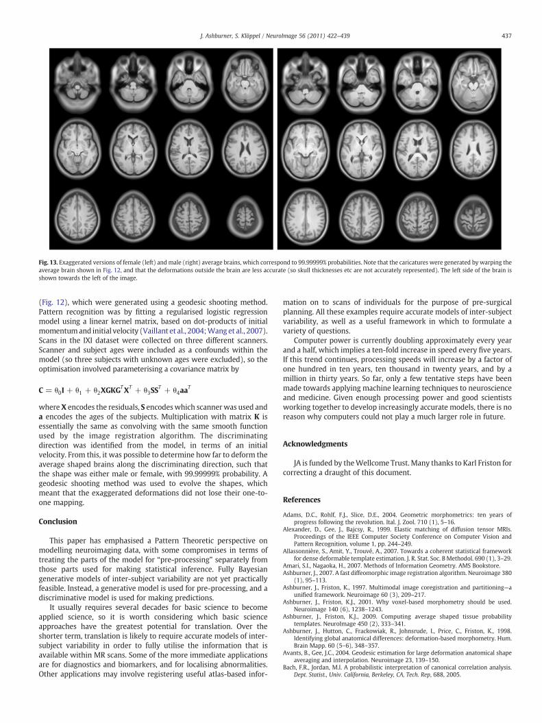
Fig. 13. Exaggerated versions of female (left) and male (right) average brains, which correspond to 99.99999% probabilities. Note that the caricatures were generated by warping theaverage brain shown in Fig. 12, and that the deformations outside the brain are less accurate (so skull thicknesses etc are not accurately represented). The left side of the brain isshown towards the left of the image.

437J. Ashburner, S. Klöppel / NeuroImage 56 (2011) 422–439

(Fig. 12), which were generated using a geodesic shooting method.Pattern recognition was by fitting a regularised logistic regressionmodel using a linear kernel matrix, based on dot-products of initialmomentumand initial velocity (Vaillant et al., 2004;Wang et al., 2007).Scans in the IXI dataset were collected on three different scanners.Scanner and subject ages were included as a confounds within themodel (so three subjects with unknown ages were excluded), so theoptimisation involved parameterising a covariance matrix by

C = θ0I + θ1 + θ2XGKGTXT + θ3SS

T + θ4aaT

whereX encodes the residuals, S encodeswhich scannerwas used anda encodes the ages of the subjects. Multiplication with matrix K isessentially the same as convolving with the same smooth functionused by the image registration algorithm. The discriminatingdirection was identified from the model, in terms of an initialvelocity. From this, it was possible to determine how far to deform theaverage shaped brains along the discriminating direction, such thatthe shape was either male or female, with 99.99999% probability. Ageodesic shooting method was used to evolve the shapes, whichmeant that the exaggerated deformations did not lose their one-to-one mapping.

Conclusion

This paper has emphasised a Pattern Theoretic perspective onmodelling neuroimaging data, with some compromises in terms oftreating the parts of the model for “pre-processing” separately fromthose parts used for making statistical inference. Fully Bayesiangenerative models of inter-subject variability are not yet practicallyfeasible. Instead, a generative model is used for pre-processing, and adiscriminative model is used for making predictions.

It usually requires several decades for basic science to becomeapplied science, so it is worth considering which basic scienceapproaches have the greatest potential for translation. Over theshorter term, translation is likely to require accurate models of inter-subject variability in order to fully utilise the information that isavailable within MR scans. Some of the more immediate applicationsare for diagnostics and biomarkers, and for localising abnormalities.Other applications may involve registering useful atlas-based infor-

mation on to scans of individuals for the purpose of pre-surgicalplanning. All these examples require accurate models of inter-subjectvariability, as well as a useful framework in which to formulate avariety of questions.

Computer power is currently doubling approximately every yearand a half, which implies a ten-fold increase in speed every five years.If this trend continues, processing speeds will increase by a factor ofone hundred in ten years, ten thousand in twenty years, and by amillion in thirty years. So far, only a few tentative steps have beenmade towards applying machine learning techniques to neuroscienceand medicine. Given enough processing power and good scientistsworking together to develop increasingly accurate models, there is noreason why computers could not play a much larger role in future.

Acknowledgments

JA is funded by theWellcome Trust. Many thanks to Karl Friston forcorrecting a draught of this document.

References

Adams, D.C., Rohlf, F.J., Slice, D.E., 2004. Geometric morphometrics: ten years ofprogress following the revolution. Ital. J. Zool. 710 (1), 5–16.

Alexander, D., Gee, J., Bajcsy, R., 1999. Elastic matching of diffusion tensor MRIs.Proceedings of the IEEE Computer Society Conference on Computer Vision andPattern Recognition, volume 1, pp. 244–249.

Allassonnière, S., Amit, Y., Trouvé, A., 2007. Towards a coherent statistical frameworkfor dense deformable template estimation. J. R. Stat. Soc. B Methodol. 690 (1), 3–29.

Amari, S.I., Nagaoka, H., 2007. Methods of Information Geometry. AMS Bookstore.Ashburner, J., 2007. A fast diffeomorphic image registration algorithm. Neuroimage 380

(1), 95–113.Ashburner, J., Friston, K., 1997. Multimodal image coregistration and partitioning—a

unified framework. Neuroimage 60 (3), 209–217.Ashburner, J., Friston, K.J., 2001. Why voxel-based morphometry should be used.

Neuroimage 140 (6), 1238–1243.Ashburner, J., Friston, K.J., 2009. Computing average shaped tissue probability

templates. NeuroImage 450 (2), 333–341.Ashburner, J., Hutton, C., Frackowiak, R., Johnsrude, I., Price, C., Friston, K., 1998.

Identifying global anatomical differences: deformation-based morphometry. Hum.Brain Mapp. 60 (5–6), 348–357.

Avants, B., Gee, J.C., 2004. Geodesic estimation for large deformation anatomical shapeaveraging and interpolation. Neuroimage 23, 139–150.

Bach, F.R., Jordan, M.I. A probabilistic interpretation of canonical correlation analysis.Dept. Statist., Univ. California, Berkeley, CA, Tech. Rep, 688, 2005.

438 J. Ashburner, S. Klöppel / NeuroImage 56 (2011) 422–439

Baloch, S., Davatzikos, C., 2009. Morphological appearance manifolds in computationalanatomy: groupwise registration and morphological analysis. Neuroimage 450(1S1), 73–85.

Baron-Cohen, S., 2002. The extreme male brain theory of autism. Trends Cogn. Sci. 60(6), 248–254.

Beckmann, C.F., Smith, S.M., 2004. Probabilistic independent component analysis forfunctionalmagnetic resonance imaging. IEEE Trans.Med. Imaging 230 (2), 137–152.

Beg, M.F., Khan, A., 2006. Computing an average anatomical atlas using LDDMM andgeodesic shooting. 3rd IEEE International Symposium on Biomedical Imaging: Nanoto Macro, pp. 1116–1119.

Beg, M.F., Miller, M.I., Trouvé, A., Younes, L., 2005. Computing large deformation metricmappings via geodesic flows of diffeomorphisms. Int. J. Comput. Vis. 610 (2),139–157.

Behrens, T.E.J., Johansen-Berg, H., Woolrich, M.W., Smith, S.M., Wheeler-Kingshott, C.A.M., Boulby, P.A., Barker, G.J., Sillery, E.L., Sheehan, K., Ciccarelli, O., et al., 2003. Non-invasive mapping of connections between human thalamus and cortex usingdiffusion imaging. Nat. Neurosci. 60 (7), 750–757.

Behrens, T.E.J., Jenkinson, M., Robson, M.D., Smith, S.M., Johansen-Berg, H., 2006. Aconsistent relationship between local white matter architecture and functionalspecialisation in medial frontal cortex. Neuroimage 300 (1), 220–227.

Behrens, T.E.J., Berg, H.J., Jbabdi, S., Rushworth, M.F.S., Woolrich, M.W., 2007.Probabilistic diffusion tractography with multiple fibre orientations: what can wegain? Neuroimage 340 (1), 144–155.

Bell, A.J., Sejnowski, T.J., 1995. An information-maximization approach to blindseparation and blind deconvolution. Neural Comput. 70 (6), 1129–1159.

Bishop, C.M., 1999. Variational principal components. Artificial Neural Networks.ICANN 99. Ninth International Conference on (Conf. Publ. No. 470), volume 1.

Bishop, C.M., Lasserre, J., 2007. Generative or discriminative? Getting the best of bothworlds. Bayesian Stat. 8, 3–24.

Bishop, C.M., et al., 2006. Pattern Recognition and Machine Learning. New York,Springer.

Bookstein, F.L., 1996. Biometrics and brain maps: the promise of the morphometricsynthesis. Neuroinformatics: an Overview of the Human Brain Project.

Bookstein, F.L., 1997. Morphometric Tools for Landmark Data: Geometry and Biology.Cambridge Univ. Pr.

Boser, B.E., Guyon, I.M., Vapnik, V.N., 1992. A training algorithm for optimal marginclassifiers. Proceedings of the Fifth Annual Workshop on Computational LearningTheory. ACM New York, NY, USA, pp. 144–152.

Bro-Nielsen, M., Cotin, S., 1996. Real-time volumetric deformable models for surgerysimulation using finite elements and condensation. Computer Graphics Forum,volume 15, pp. 57–66.

Butcher, J., 2007. Alzheimer's researchers open the doors to data sharing. Lancet Neurol.60 (6), 480–481.

Chance, S.A., Esiri, M.M., Crow, T.J., 2005. Macroscopic brain asymmetry is changedalong the antero-posterior axis in schizophrenia. Schizophr. Res. 740 (2–3),163–170.

Chapelle, O., Schölkopf, B., Zien, A., 2006. Semi-Supervised Learning.Christensen, G.E., Rabbitt, R.D., Miller, M.I., Joshi, S.C., Grenander, U., Coogan, T.A., Van

Essen, D.C., 1995. Topological properties of smooth anatomic maps. Informationprocessing in medical imaging, pp. 101–112.

Cotter, C.J., Holm, D.D., Singular solutions, momentummaps and computational anatomy.Arxiv preprint nlin.SI/0605020, 2006.

Cristianini, N., Shawe-Taylor, J., 2000. An Introduction to Support Vector Machines: andOther Kernel-Based Learning Methods. Cambridge Univ Pr.

Csete, M.E., Doyle, J.C., 2002. Reverse Engineering of Biological Complexity.da Fontoura Costa, L., Cesar, R.M., 2001. Shape Analysis and Classification: Theory and

Practice. CRC.Davatzikos, C., Shen, D., Lao, Z., Xue, Z., Karacali, B., 2004. Morphological classification of

medical images using nonlinear support vector machines. IEEE InternationalSymposium on Biomedical Imaging: Nano to Macro, pp. 587–590.

Davatzikos, C., Fan, Y., Wu, X., Shen, D., Resnick, S.M., 2008. Detection of prodromalAlzheimer's disease via pattern classification of magnetic resonance imaging.Neurobiol. Aging 290 (4), 514–523.

Davies, R., Twining, C., Taylor, C., 2008. Statistical Models of Shape: Optimisation andEvaluation. Springer-Verlag New York Inc.

Dryden, I.L., Mardia, K.V., 1998. Statistical Shape Analysis. Wiley, New York.Duda, R.O., Hart, P.E., Stork, D.G., 2001. Pattern Classification. Wiley, New York.Elstein, A.S., Schwarz, A., 2002. Clinical Problem Solving and Diagnostic Decision

Making: Selective Review of the Cognitive Literature.Fan, Y., Shen, D., Davatzikos, C., 2005. Classification of structural images via high-

dimensional image warping, robust feature extraction, and SVM: Lect. NotesComput. Sci., 3749, p. 1.

Fletcher, P.C., Dolan, R.J., Shallice, T., Frith, C.D., Frackowiak, R.S.J., Friston, K.J., 1996. Ismultivariate analysis of PET data more revealing than the univariate approach?Evidence from a study of episodic memory retrieval. NeuroImage 30 (3), 209–215.

Friston, K., Mattout, J., Trujillo-Barreto, N., Ashburner, J., Penny, W., 2007. Variationalfree energy and the Laplace approximation. NeuroImage 340 (1), 220–234.

Friston, K., Chu, C., Mourão-Miranda, J., Hulme, O., Rees, G., Penny, W., Ashburner, J.,2008. Bayesian decoding of brain images. Neuroimage 390 (1), 181–205.

Friston, K.J., Ashburner, J., 2004. Generative and recognition models for neuroanatomy.NeuroImage 230 (1), 21–24.

Friston, K.J., Holmes, A.P., Worsley, K.J., Poline, J.P., Frith, C.D., Frackowiak, R.S.J., et al.,1994. Statistical parametric maps in functional imaging: a general linear approach.Hum. Brain Mapp. 20 (4), 189–210.

Friston, K.J., Poline, J.B., Holmes, A.P., Frith, C.D., Frackowiak, R.S.J., 1996. A multivariateanalysis of PET activation studies. Hum. Brain Mapp. 40 (2).

Gerardin, E., Chételat, G., Chupin, M., Cuingnet, R., Desgranges, B., Kim, H.S.,Niethammer, M., Dubois, B., Lehéricy, S., Garnero, L., et al., 2009. Multidimensionalclassification of hippocampal shape features discriminates Alzheimer's disease andmild cognitive impairment from normal aging. Neuroimage.

Ghahramani, Z., Beal, M.J., 2000. Variational inference for Bayesian mixtures of factoranalysers: Adv. Neural. Inf. Process. Syst., 12, pp. 449–455.

Golland, P., 2002. Discriminative direction for kernel classifiers. Adv. Neural Inf. Proces.Syst. 1, 745–752.

Golland, P., Grimson, W.E.L., Shenton, M.E., Kikinis, R., 2001. Deformation analysis forshape based classification. Lect. Notes Comput. Sci. 517–530.

Golland, P., Grimson, W.E.L., Shenton, M.E., Kikinis, R., 2005. Detection and analysis ofstatistical differences in anatomical shape. Med. Image Anal. 90 (1), 69–86.

Grenander, U., Miller, M., 2007. Pattern Theory: from Representation to Inference.Oxford University Press, USA.

Grenander, U., Miller, M.I., 1998. Computational anatomy: an emerging discipline.Q. Appl. Math. 560 (4), 617–694.

Guimond, A., Guttmann, C.R.G.,Warfield, S.K.,Westin, C.F., 2002. Deformable registrationof DT-MRI data based on transformation invariant tensor characteristics. Proc. ISBI,volume 2.

Hand, D.J., 2001. Measuring diagnostic accuracy of statistical prediction rules. Stat.Neerl. 550 (1), 3–16.

Hinton, G.E., Osindero, S., Teh, Y.W., 2006. A fast learning algorithm for deep belief nets.Neural Comput. 180 (7), 1527–1554.

Hirsch, J.E., 2007. Does the h index have predictive power? Proc. Natl Acad. Sci. U. S. A.1040 (49), 19193.

Holub, A.D., Welling, M., Perona, P., 2008. Hybrid generative-discriminative visualcategorization. Int. J. Comput. Vis. 770 (1), 239–258.

Hoyer, P.O., Janzing, D., Mooij, J., Peters, J., Scholkopf, B., 2009. Nonlinear causaldiscovery with additive noise models. Adv. Neural. Inf. Process. Syst. 21, 689–696.

Huxley, J., 1993. Problems of Relative Growth. Johns Hopkins University Press.Jaakkola, T., Diekhans, M., Haussler, D., 2000. A discriminative framework for detecting

remote protein homologies. J. Comput. Biol. 70 (1–2), 95–114.Jaynes, E.T., Bretthorst, G.L., 2003. Probability Theory: the Logic of Science. Cambridge

University Press, Cambridge UK.Johansen-Berg, H., Behrens, T.E.J., Sillery, E., Ciccarelli, O., Thompson, A.J., Smith, S.M.,

Matthews, P.M., 2005. Functional–anatomical validation and individual variation ofdiffusion tractography-based segmentation of the human thalamus. Cereb. Cortex150 (1), 31–39.

Joshi, S., Davis, B., Jomier, M., Gerig, G., 2004. Unbiased diffeomorphic atlas constructionfor computational anatomy. NeuroImage 23, 151–160.

Kendall, D.G., Barden, D., Carne, T.K., Le, H., 1999. Shape and Shape Theory. Wiley.Kiebel, S.J., Daunizeau, J., Phillips, C., Friston, K.J., 2008. Variational Bayesian inversion of

the equivalent current dipole model in EEG/MEG. NeuroImage 390 (2), 728–741.Kitano, H., 2002. Computational systems biology. Nature 4200 (6912), 206–210.Klein, J.C., Behrens, T.E.J., Robson, M.D., Mackay, C.E., Higham, D.J., Johansen-Berg, H.,

2007. Connectivity-based parcellation of human cortex using diffusion MRI:establishing reproducibility, validity and observer independence in BA 44/45 andSMA/pre-SMA. Neuroimage 340 (1), 204–211.

Kloppel, S., Stonnington, C.M., Barnes, J., Chen, F., Chu, C., Good, C.D., Mader, I., AnneMitchell, L., Patel, A.C., Roberts, C.C., et al., 2008a. Accuracy of dementia diagnosis—adirect comparison between radiologists and a computerized method. Brain.

Kloppel, S., Stonnington, C.M., Chu, C., Draganski, B., Scahill, R.I., Rohrer, J.D., Fox, N.C.,Jack, C.R., Ashburner, J., Frackowiak, R.S.J., 2008b. Automatic classification of MRscans in Alzheimer's disease. Brain 681 (3).

Krim, H., Yezzi, A.J., 2006. Statistics and Analysis of Shapes. Birkhauser.Lao, Z., Shen, D., Xue, Z., Karacali, B., Resnick, S.M., Davatzikos, C., 2004. Morphological

classification of brains via high-dimensional shape transformations and machinelearning methods. Neuroimage 210 (1), 46–57.

Lasserre, J.A., Bishop, C.M., Minka, T.P., 2006. Principled hybrids of generative anddiscriminative models. 2006 IEEE Computer Society Conference on ComputerVision and Pattern Recognition, volume 1.

Lee, D.D., Seung, H.S., 1999. Learning the parts of objects by non-negative matrixfactorization. Nature 4010 (6755), 788–791.

Lele, S., Richtsmeier, J.T., 2001. An invariant Approach to Statistical Analysis of Shapes.CRC Pr I Llc.

Lorenzen, P., Davis, B., Joshi, S., 2005. Unbiased atlas formation via large deformationsmetric mapping. Lect. Notes Comput. Sci. 3750, 411.

Luders, E., Steinmetz, H., Jancke, L., 2002. Brain size and grey matter volume in thehealthy human brain. Neuroreport 130 (17), 2371.

MacKay, D.J.C., 1992. The evidence framework applied to classification networks.Neural Comput. 40 (5), 720–736.

MacKay, D.J.C., 2003. Information Theory, Inference, and Learning Algorithms.Cambridge Univ Pr.

Magnin, B., Mesrob, L., Kinkingnéhun, S., Pélégrini-Issac, M., Colliot, O., Sarazin, M.,Dubois, B., Lehéricy, S., Benali, H., 2009. Support vector machine-based classifica-tion of Alzheimer's disease from whole-brain anatomical MRI. Neuroradiology 510(2), 73–83.

Makrogiannis, S., Verma, R., Karacali, B., Davatzikos, C., 2007. Anatomical equivalenceclass: a morphological analysis framework using a lossless shape descriptor. IEEETrans. Med. Imaging 26 (4), 619–631.

Marcus, D.S., Wang, T.H., Parker, J., Csernansky, J.G., Morris, J.C., Buckner, R.L., 2007. OpenAccess Series of Imaging Studies (OASIS): cross-sectional MRI data in young, middleaged, nondemented, and demented older adults. J. Cogn. Neurosci. 190 (9), 1498–1507.

Markram, H., 2006. The blue brain project. Nat. Rev. Neurosci. 70 (2), 153–160.Marsland, S., McLachlan, R., 2007. A Hamiltonian particle method for diffeomorphic

image registration. Lect. Notes Comput. Sci. 4584, 396.

439J. Ashburner, S. Klöppel / NeuroImage 56 (2011) 422–439

Martin, R.D., 1981. Relative brain size and basal metabolic rate in terrestrial vertebrates.Nature 293, 57–60.

Mazziotta, J., Toga, A., Evans, A., Fox, P., Lancaster, J., Zilles, K., Woods, R., Paus, T.,Simpson, G., Pike, B., et al., 2001. A probabilistic atlas and reference system for thehuman brain: International Consortium for Brain Mapping (ICBM). Philos. Trans. R.Soc. Lond. B Biol. Sci. 3560, 1293.

McIntosh, A.R., Bookstein, F.L., Haxby, J.V., Grady, C.L., 1996. Spatial pattern analysis offunctional brain images using partial least squares. Neuroimage 30 (3), 143–157.

Mechelli, A., Friston, K.J., Frackowiak, R.S., Price, C.J., 2005. Structural covariance in thehuman cortex. J. Neurosci. 250 (36), 8303–8310.

Miller, M., Banerjee, A., Christensen, G., Joshi, S., Khaneja, N., Grenander, U., Matejic, L.,1997. Statistical methods in computational anatomy. Stat. Meth. Med. Res. 60 (3),267.

Miller, M.I., 2004. Computational anatomy: shape, growth, and atrophy comparison viadiffeomorphisms. NeuroImage 23, 19–33.

Miller, M.I., Qiu, A., 2009. The emerging discipline of Computational FunctionalAnatomy. Neuroimage 450 (1S1), 16–39.

Miller, M.I., Trouvé, A., Younes, L., 2006. Geodesic shooting for computational anatomy.J. Math. Imaging Vis. 240 (2), 209–228.

Miller, M.I., Priebe, C.E., Qiu, A., Fischl, B., Kolasny, A., Brown, T., Park, Y., Ratnanather,J.T., Busa, E., Jovicich, J., et al., 2008. Collaborative computational anatomy: an MRImorphometry study of the human brain via diffeomorphic metric mapping. Hum.Brain Mapp. 300 (7), 2132–2141.

Mitchell, T.M., Hutchinson, R., Niculescu, R.S., Pereira, F., Wang, X., Just, M., Newman, S.,2004. Learning to decode cognitive states from brain images. Mach. Learn. 570 (1),145–175.

Mueller, S.G., Weiner, M.W., Thal, L.J., Petersen, R.C., Jack, C.R., Jagust, W., Trojanowski,J.Q., Toga, A.W., Beckett, L., 2005. Ways toward an early diagnosis in Alzheimer'sdisease: the Alzheimer's Disease Neuroimaging Initiative (ADNI). AlzheimersDement. J. Alzheimer's Assoc. 10 (1), 55–66.

Mumford, D., 1994. Neuronal architectures for pattern-theoretic problems. Large-scaleneuronal theories of the brain, pp. 125–152.

Mumford, D., 1996. Pattern theory: a unifying perspective. Perception as Bayesianinference, pp. 25–62.

Mumford, D., 2002. Pattern theory: the mathematics of perception. Proceedings of theInternational Congress of Mathematicians, volume 3.

Mumford, D., 2005. Empirical statistics and stochastic models for visual signals. NewDirections in Statistical Signal Processing: From Systems to Brain.

Oishi, K., Zilles,K., Amunts,K., Faria,A., Jiang,H., Li, X., Akhter,K.,Hua,K.,Woods,R., Toga,A.W.,et al., 2008. Human brain white matter atlas: identification and assignment of commonanatomical structures in superficial white matter. Neuroimage 430 (3), 447–457.

Park, H.J., Kubicki, M., Shenton, M.E., Guimond, A., McCarley, R.W., Maier, S.E., Kikinis, R.,Jolesz, F.A., Westin, C.F., 2003. Spatial normalization of diffusion tensor MRI usingmultiple channels. Neuroimage 200 (4), 1995–2009.

Penny, W.D., Stephan, K.E., Mechelli, A., Friston, K.J., 2004. Comparing dynamic causalmodels. NeuroImage 220 (3), 1157–1172.

Pereira, F., Mitchell, T., Botvinick, M., 2009. Machine learning classifiers and fMRI: atutorial overview. Neuroimage 450 (1S1), 199–209.

Petersson, K.M., Nichols, T.E., Poline, J.B., Holmes, A.P., 1999. Statistical limitations infunctional neuroimaging. I. Non-inferential methods and statistical models. Philos.Trans. R. Soc. Biol. Sci. 3540 (1387), 1239–1260.

Qiu, A., Miller, M.I., 2008. Multi-structure network shape analysis via normal surfacemomentum maps. Neuroimage 420 (4), 1430–1438.

Rasmussen, C.E., Quinonero-Candela, J., 2005. Healing the relevance vector machinethrough augmentation.Machine Learning-InternationalWorkshopThenConference,volume 22, p. 689.

Rasmussen, C.E., Williams, C.K.I., 2006. Gaussian Processes for Machine Learning.Springer.

Rilling, J.K., 2006. Human and nonhuman primate brains: are they allometrically scaledversions of the same design? Evol. Anthropol.: Issues News Rev. 150 (2).

Roweis, S., Ghahramani, Z., 1999. A unifying review of linear Gaussian models. NeuralComput. 110 (2), 305–345.

Ruiz-Alzola, J., Westin, C.F., Warfield, S.K., Alberola, C., Maier, S., Kikinis, R., 2002.Nonrigid registration of 3D tensor medical data. Med. Image Anal. 60 (2), 143–161.

Sabuncu, M.R., Singer, B.D., Conroy, B., Bryan, R.E., Ramadge, P.J., Haxby, J.V., 2010.Function-based intersubject alignment of human cortical anatomy. Cereb. Cortex20, 130–140.

Salimi-Khorshidi, G., Smith, S.M., Keltner, J.R., Wager, T.D., Nichols, T.E., 2009. Meta-analysis of neuroimaging data: a comparison of image-based and coordinate-basedpooling of studies. Neuroimage 450 (3), 810–823.

Saxe, R., Brett, M., Kanwisher, N., 2006. Divide and conquer: a defense of functionallocalizers. Neuroimage 300 (4), 1088–1096.

Schmah, T., Hinton, G.E., Zemel, R.S., Small, S.L., Strother, S., 2008. Generative versusdiscriminative training of RBMs for classification of fMRI images. NIPS.

Schölkopf, B., Smola, A.J., 2002. Learning with Kernels: Support Vector Machines,Regularization, Optimization, and Beyond. the MIT Press.

Seeley, W.W., Crawford, R.K., Zhou, J., Miller, B.L., Greicius, M.D., 2009. Neurodegen-erative diseases target large-scale human brain networks. Neuron 620 (1), 42–52.

Small, C.G., 1996. The Statistical Theory of Shape. Springer Verlag.Smith, S.M., Fox, P.T., Miller, K.L., Glahn, D.C., Fox, P.M., Mackay, C.E., Filippini, N.,

Watkins, K.E., Toro, R., Laird, A.R., et al., 2009. Correspondence of the brain'sfunctional architecture during activation and rest. Proc. Natl Acad. Sci. U. S. A. 1060(31), 13040.

Stephan, K.E., Kamper, L., Bozkurt, A., Burns, G., Young, M.P., Kotter, R., 2001. Advanceddatabase methodology for the Collation of Connectivity data on the Macaque brain(CoCoMac). Philos. Trans. R. Soc. Lond. B Biol. Sci. 356, 1159–1186.

Thompson, D., Bonner, J.T., 1942. On Growth and Form. Cambridge University Press,Cambridge.

Tipping, M.E., 2001. Sparse Bayesian learning and the relevance vector machine. Journalof Machine Learning Research 1, 211–244.

Tipping, M.E., Bishop, C.M., 1999a. Mixtures of probabilistic principal componentanalyzers. Neural Comput. 110 (2), 443–482.

Tipping, M.E., Bishop, C.M., 1999b. Probabilistic principal component analysis. J. R. Stat.Soc. B Stat. Methodol. 611–622.

Trouvé, A., Younes, L., 2005. Metamorphoses through lie group action. Found. Comput.Math. 50 (2), 173–198.

Trouvé, A., Yu, Y., 2001. Metric similarities learning through examples: an application toshape retrieval. Lect. Notes Comput. Sci. 50–62.

Vaillant, M., Miller, M.I., Younes, L., Trouvé, A., 2004. Statistics on diffeomorphisms viatangent space representations. NeuroImage 23, 161–169.

Van Horn, J.D., Toga, A.W., 2009. Is it time to re-prioritize neuroimaging databases anddigital repositories? Neuroimage.

Van Leemput, K., Maes, F., Vandermeulen, D., Suetens, P., 1999. Automated model-based tissue classification of MR images of the brain. IEEE Trans. Med. Imaging 180(10), 897–908.

Vapnik, V.N., 1999. An overview of statistical learning theory. IEEE Transact. NeuralNetw. 100 (5), 988–999.

Vemuri, P., Gunter, J.L., Senjem, M.L., Whitwell, J.L., Kantarci, K., Knopman, D.S., Boeve,B.F., Petersen, R.C., Jack, C.R., 2008. Alzheimer's disease diagnosis in individualsubjects using structural MR images: validation studies. Neuroimage 390 (3),1186–1197.

Wang, L., Beg, F., Ratnanather, T., Ceritoglu, C., Younes, L., Morris, J.C., Csernansky, J.G.,Miller, M.I., 2007. Large deformation diffeomorphism and momentum basedhippocampal shape discrimination in dementia of the Alzheimer type. IEEE Trans.Med. Imaging 260 (4), 462–470.

Watanabe, S., 1969. Knowing and Guessing: a Quantitative Study of Inference andInformation. John Wiley & Sons.

West, G.B., Brown, J.H., 2005. The Origin of Allometric Scaling Laws in Biology fromGenomes to Ecosystems: Towards a Quantitative Unifying Theory of Biologicalstructure and Organization.

West, G.B., Brown, J.H., Enquist, B.J., 2001. A general model for ontogenetic growth.Nature 4130 (6856), 628–631.

Williams, C.K.I., Barber, D., 1998. Bayesian classification with Gaussian processes. IEEETrans. Pattern Anal. Mach. Intell. 200 (12), 1342–1351.

Williams, C.K.I., Rasmussen, C.E., 1996. Gaussian processes for regression. Adv. Neural.Inf. Process. Syst. 8.

Woods, R.P., 2003. Characterizing volume and surface deformations in an atlasframework: theory, applications, and implementation. NeuroImage 180 (3),769–788.

Wright, I.C., McGuire, P.K., Poline, J.B., Travere, J.M., Murray, R.M., Frith, C.D.,Frackowiak, R.S.J., Friston, K.J., 1995. A voxel-based method for the statisticalanalysis of gray and white matter density applied to schizophrenia. Neuroimage 20(4), 244–252.

Xu, L., Liu, J., Adali, T., Calhoun, V.D., 2008. Source based morphometry using structuralMRI phase images to identify sources of gray matter and white matter relativedifferences in schizophrenia versus controls. IEEE International Conference onAcoustics, Speech and Signal Processing, 2008: ICASSP 2008, pp. 533–536.

Younes, L., 2007. Jacobi fields in groups of diffeomorphisms and applications. Q. Appl.Math. 650 (1), 113–134.

Younes, L., Qiu, A., Winslow, R.L., Miller, M.I., 2008. Transport of relational structures ingroups of diffeomorphisms. J. Math. Imaging Vis. 320 (1), 41–56.

Younes, L., Arrate, F., Miller, M.I., 2009. Evolutions equations in computational anatomy.Neuroimage 450 (1S1), 40–50.

Zhang, H., Yushkevich, P.A., Alexander, D.C., Gee, J.C., 2006. Deformable registration ofdiffusion tensor MR images with explicit orientation optimization. Med. ImageAnal. 100 (5), 764–785.

Zhang, K., Sejnowski, T.J., 2000. A universal scaling law between gray matter and whitematter of cerebral cortex. Proc. Natl Acad. Sci. U. S. A. 970 (10), 5621–5626.

Zhu, X., Goldberg, A.B., 2009. Introduction to Semi-Supervised Learning. Synth. Lect.Artif. Intell. Mach. Learn. 30 (1), 1–130.

Zou, K.H., O'Malley, A.J., Mauri, L., 2007. Receiver-operating characteristic analysis forevaluating diagnostic tests and predictive models. Circulation 1150 (5), 654.