Embed Size (px)
Citation preview
Multivariate Dynamic Tobit Model
Yin LiaoSchool of Economics and Finance
Queensland University of TechnologyAustralia
Heather M. Anderson and Farshid VahidDepartment of Econometrics and Business Statistics
Monash UniversityAustralia ∗
March 2014
Abstract
This paper studies a generalization of a Tobit model for modelling multiple time series
that are mixed discrete and continuous. We propose an estimation method for this model
based on a modified Kalman filter. We use this model for modelling the contribution of
price jumps to realized volatility in three Chinese pharmaceutical stocks. Out of sample
forecast analysis shows that separate multivariate factor models for the two volatility
components outperform a single multivariate factor model of realized volatility.
Keywords: Multivariate Dynamic Tobit, Common Factors, Forecasting, Realized Volatil-ity, Jumps.
JEL classification: C13, C32, C52, C53, G17, G32
∗E-mail: [email protected], [email protected], [email protected]

1 Introduction
We often encounter variables that are mixed discrete and continuous, in the sense that by
definition they cannot be lower (or higher) than a certain threshold, and we observe a pile
up at the threshold. For example, rainfall can only be zero or positive, but it has a positive
probability at zero, wage of a working age person can only be zero or positive, with a positive
probability mass at zero. Stock prices are subject to occasional jumps, and although these
jumps are not predictable, their squares that contribute to the volatility of stock returns, may
be predictable. These squared jumps are random variables that are either zero or positive,
with a positive mass at zero. The question that this paper investigates is time series models
for multiple mixed discrete-continuous variable of this kind.
An appropriate modelling framework for mixed discrete-continuous random variables is
the tobit model proposed by Tobin (1958), in which the observed variables is linked to an
underlying continuous random variable, whose conditional distribution given a set of indepen-
dent variables is Gaussian. In this model, the observed variable is equal to the underlying
variable whenever the latter is positive, and is zero otherwise. The dynamic version of the
tobit model has been studied in Zeger and Brookmeyer (1986) and Mxxxx .... Mxxx assumes a
finite autoregressive model for the underlying variable, and evaluates the likelihood separately
depending on the sequence of zero and non-zero observations in the likelihood function. Zeger
and Brookmeyer (1986) suggest a pseudo-likelihood approach that amounts to recursively re-
placing all censored observations with their expectation given that they are in the censoring
region (above or below a threshold as the case may be), and then fitting an autoregressive
model to the resulting time series. This method is computationally quite convenient, but, as
we show later, it does not provide consistent estimates of the true parameters. In this paper,
we provide an alternative that can be easily generalized to a multivariate setting.
The generalization of dynamic tobit model to the multivariate case involves several compli-
cations. Firstly, the derivations of mean and variance of truncated multivariate normal random
vectors are more complicated than the univariate case, but these derivations are available in
print (see, for example, McGill (1992)). Secondly, to stay practically relevant, we must allow
some elements of the vector to be censored while other are not. Moreover, since in all practical
applications we want to allow for correlation among the elements of the random vector, the
non-censored elements carry information about the censored elements. Hence, we will need
to compute mean and variance of the subvector of censored elements conditional on the other
elements of a multivariate normal distribution with a given correlation structure. Finally,
when we consider observing such vector of variables over time, the censored subvector changes
at each time period, and the computer code must be clever enough to apply the appropri-
ate formulae effi ciently. In presenting our generalization, we pay particular attention to the
programming aspect as well.
With the advances in information technology, we increasingly have access to time series
2
of interdependent censored variables, and it is quite conceivable that modelling the dynamics
of such variables jointly could provide better forecasts than univariate dynamic models. For
non-censored time series, a convenient multivariate dynamic model is a vector autoregressive
(VAR) model (see, e.g. Lütkepohl (1993)). However, as the number of variables that are
modelled jointly increases, the number of parameters in a VAR increases sharply and its
benefit as a forecasting device deteriorates. In such situations, reduced rank VARs or dynamic
factor models, which relate the dynamics of multiple time series to a small number of common
factors, show an advantage over unrestricted VARs for forecasting, see, among others, Velu
et al. (1986), Ahn and Reinsel (1988), Vahid and Issler (2002) and Anderson and Vahid (2007).
In multivariate modelling of time series with similar dynamics, factor models have been
shown to be an effective way of dealing with proliferation of parameters in an unrestricted
time series model such as a vector autoregressive model. In economics and in finance, such
models have some theoretical justifications Merton (1976), and they have also shown to lead
to reasonable success in providing better forecasts than alternative time series models ??.It is reasonable to expect that such dynamic models could be appropriate for modelling the
dynamics of continuous variables that underlie a multivariate tobit model.
2 The statistical model and the proposed estimator
In the remainder of the paper, all scalar random variables are denoted by lower case letters,
all vectors by boldface lower case letters and all matrices by upper case letters.
Let yt = (y1t, y2t, . . . , ynt)′ be a vector of n observed time series. We assume that each
element of yt is related to the corresponding element of an underlying vector of continuous
random variables y∗t = (y∗1t, y∗2t, . . . , y
∗nt)′ using the tobit mechanism, i.e.,
yit =
y∗it if y∗it > 0
0 otherwise, for i = 1, ..., n. (1)
The censoring threshold is assumed to be zero here for the ease of notation and without loss of
generality. The dynamics of the vector of random variables y∗t are represented in state space
form with a measurement equation given by
y∗t = µ+Hst + ut (2)
and a state transition equation given by
st = F st−1 + vt, (3)
where µ is an n × 1 vector, H is an n × k matrix and F is an k × k matrix of constants,and ut and vt are n × 1 and k × 1 vectors of random variables with E (ut) = 0, E (vt) = 0,
E(utv
′t−j
)= 0 for all j, E
(utu
′t−j
)= Ω for j = 0 and zero otherwise, and E
(vtv
′t−j
)= Q
3
for j = 0 and zero otherwise. Some elements of ut and vt can be zero. We further assume that
random elements of ut and vt are normally distributed, which together with the assumptions
on covariances imply statistical independence. This formulation is rich enough to encompass
VAR and dynamic factor dynamics for the random vector y∗t . The dimension of the state
vector, the free parameters in µ, H and F and the structure of the error vectors are determined
by our assumptions about a reasonable dynamic model for y∗t . For example, if we assume that
the underlying dynamic model for y∗t is a stationary VAR of order 2
y∗t = c+A1y∗t−1 +A2y
∗t−2 + εt,
then:
st =
(y∗ty∗t−1
), H = (In, 0n×n) , ut = 0,
F =
(A1 A2
In 0n×n
), and vt =
(εt
0
).
Another useful example is when all elements of y∗t are assumed to share a common dynamic
factor ft besides each having their idiosyncratic dynamic components, which for ease of nota-
tion assumed to be autoregressive of order 1:
y∗t = µ+
α1
...
αn
ft +
η1t...
ηnt
ft = ρft−1 + ζt
ηit = φiηit−1 + ξit, i = 1, . . . , n,
in which case
st =
(ft
ηt
), H = (α,In) , ut = 0,
F =
(ρ 01×n
0n×1 diag (φ1, . . . , φn)
), and vt =
(ζt
ξt
).
If y∗t , t = 1, . . . , T were observed, the quasi-maximum likelihood estimator for the parame-
ters of the model could be estimated by maximizing the Gaussian likelihood with the help of
the standard Kalman filter, or in the VAR case by ordinary least squares regression equation
by equation. However, the elements of y∗t are only observed when they are positive, so we
have to modify the standard estimation procedure to accommodate the information behind
the censoring mechanism.
4
2.1 The log-likelihood function
Consider the random vector yt with joint density denoted by D (yt) . Consider any arbitrary
partition of yt into y1t and y2t. Then by Bayes theorem we have:
D (yt) = D (y1t | y2t)×D (y2t) = D (y2t | y1t)×D (y1t)
where D (A | B) denotes the conditional density of A given B. We denote joint, marginal and
conditional density functions with the letter D, although each may have a different number
of arguments and may belong to a different family of distributions. The likelihood function is
the joint density evaluated at the observed realization of yt, and this can be evaluated either
by evaluating the joint density D (yt) , or by using either of the formulations D (y1t | y2t) ×D (y2t) or D (y2t | y1t) ×D (y1t) . These facts are well-known and are often used in practice
because we can then use univariate densities rather than multivariate densities when evaluating
the likelihood. We note that one can choose which formulation to use after observing the
realization yt. For example, one could place all non-positive elements of yt in y1t and the
rest in y2t. This means that for a different realization, the partition might be different, but
the likelihood would still be calculated correctly. This type of partitioning does not have any
computational advantage when dealing with continuous random variables, but it will simplify
computations of the likelihood when working with tobit type random variables generated by
(1).
The log-likelihood function for yt, t = 1, . . . , T is
lnL (θ | yT ,yT−1, . . . ,y1) = lnD (yT ,yT−1, . . . ,y1; θ)
=
T∑t=1
lnD (yt | It−1; θ) ,
whereD (.) is the joint probability density function, D (. | It−1) is the conditional density given
the observed information at time t − 1 and θ is the vector of model parameters. For each t,
some of the elements of yt can be exactly zero, and the rest will be strictly positive. Using the
argument stated above, it is convenient for us to partition the elements in the vector yt ex-
post into two smaller vectors y0t and y
+t , that contain the zero and strictly positive elements
of yt respectively.1 Then, for computational convenience we calculate the log-likelihood of
observation t using
lnD (yt | It−1) = lnD(y0t | y+
t , It−1
)+ lnD
(y+t | It−1
).
Recalling that the realization yt (and hence y0t and y
+t ) is determined by the realization of the
underlying continuous random vector y∗t , we partition y∗t ex-post into subvectors that we will
1We do not partition if elements of yt happen to be all positive, or all zero. These cases are discussed in
further detail below.
5
call y∗≤0t and y∗+t that have an exact correspondence to the partition of yt into y0
t and y+t . It
is clear that D(y+t | It−1
)= D
(y∗+t | It−1
). Further, although y∗≤0
t is not observed, the tobit
structure implies thatD(y0t | y+
t , It−1
)=∫ 0−∞D
(y∗≤0t | y∗+t , It−1
)dy∗≤0
t = Pr(y∗≤0t ≤ 0 | y∗+t , It−1
),
where the integral sign here is a multiple integral that depends on the dimension of y∗≤0t . Thus,
we can compute the log-likelihood of observation t as
lnD (yt | It−1) = ln Pr(y∗≤0t ≤ 0 | y∗+t , It−1
)+ lnD
(y∗+t | It−1
). (4)
We emphasize that the partition of y∗t into y∗≤0t and y∗+t is done ex-post and it is completely
determined by the realization of yt. Although the size of these vectors and their constituent
elements will change with t, (4) offers computational convenience, and this will allow us to
evaluate the log-likelihood contribution of each observation in turn, for t = 1, . . . , T.
While the structure of the model implies thatD(y∗t | y∗t−1,y
∗t−2, . . .
)is normal,D (y∗t | It−1) =
D (y∗t | yt−1,yt−2, . . .) , will not be normal. Our estimation strategy is to determine the mean
and variance of D (y∗t | It−1) via a modified Kalman filter, and approximate D (y∗t | It−1) with
a normal distribution. To explain the mechanics of this, we need to introduce additional no-
tation. This additional notation is particularly useful for readers who would want to write
computer code to use our model, and it simply rearranges the vector of observations into
partitions that change with every observation and allows us to track the relevant conditional
means and variances as the filter works through the data.
Let w0t and w+t denote the sets of indices for elements of yt that are observed to be zero
and positive respectively, i.e. w0t = i : y∗it ≤ 0 and w+t = i : y∗it > 0 , and let n0t and
n+t denote the cardinality of w0t and w+t. Either of these sets (but not both) can be empty
and their intersection is empty, but w0t ∪ w+t = 1, 2, . . . , n , implying that n0t + n+t = n.
We take n0t rows of the n × n identity matrix corresponding to the indices in w0t and stack
them into a matrix X0t and then we stack the other n+t rows of the identity matrix into a
matrix X+t. This ensures that X0ty∗t selects the n0t subvector of y∗t whose elements are all
non-positive and X+ty∗t selects all n+t strictly positive elements of y∗t . It is important to note
that X0t and X+t are simply selection matrices that are completely determined ex-post by
the realization of yt, and that they do not introduce another source of randomness into the
analysis. Indeed, X0ty∗t is equivalent to y
∗≤0t and X+ty
∗t is equivalent to y
∗+t . With this new
notation, we can rewrite (4) as
lnD (yt | It−1) = ln Pr (X0ty∗t ≤ 0 | X+ty
∗t , It−1) + lnD (X+ty
∗t | It−1) .
We use the notation y∗t|t−1 and Gt|t−1 to denote the mean and variance of y∗t | It−1, and
then the means of X0ty∗t | It−1 and X+ty
∗t | It−1 will be X0ty
∗t|t−1 and X+ty
∗t|t−1, their
variances will be X0tGt|t−1X′0t and X+tGt|t−1X
′+t, and their covariance will be X0tGt|t−1X
′+t.
If we now treatD (y∗t | It−1) as normally distributed, then the densityD (X0ty∗t | X+ty
∗t , It−1)
6
will have a conditional mean and variance given by
E (X0ty∗t | X+ty
∗t , It−1) = X0ty
∗t|t−1 (5)
+X0tGt|t−1X′+t
(X+tGt|t−1X
′+t
)−1(X+ty
∗t −X+ty
∗t|t−1
)and
V ar (X0ty∗t | X+ty
∗t , It−1) = X0tGt|t−1X
′0t (6)
−X0tGt|t−1X′+t
(X+tGt|t−1X
′+t
)−1X+tGt|t−1X
′0t.
We use these latter expressions to estimate Pr (X0ty∗t ≤ 0 | X+ty
∗t , It−1) . The second piece
of the likelihood, i.e. D (X+ty∗t | It−1) is the PDF of an n+t dimensional normally distributed
random variable with mean X+ty∗t|t−1 and variance X+tGt|t−1X
′+t, evaluated at X+tyt. The
quantities y∗t|t−1 and Gt|t−1 are conditional on the structure of the model and the data, and are
computed recursively using a slight modification of the Kalman filter that we explain below.
2.1.1 Kalman filter modification
We initiate the Kalman filter by using the unconditional mean and variance of the state vector
implied by the model, i.e. s0|0 = 0 and vec(P0|0) = (I − F ⊗ F )−1vec(Q) in the state space
model outlined in sub-section ??. The prediction step of the Kalman filter does not need anymodification because for any t, given st−1|t−1 and Pt−1|t−1 the structure of the model implies
what st|t−1, Pt|t−1, y∗t|t−1 and Gt|t−1 should be. However, at time t we observe a yt that is
generated by the tobit mechanism in equation (1) and this might contain some zeros. Treating
the zeros as missing values and using a multivariate version of the Kalman filter algorithm
suggested for irregularly observed time series (see Brockwell and Davis, 1991, section 12.3)
would not be appropriate because the zeros are not independent of positive observations.
Moreover, a zero carries the information that this element of y∗t is negative, whereas for an
irregularly observed time series a missing value is treated as if it could have any value, positive
or negative. Treating zeros at face value and using standard Kalman recursions would produce
quasi-maximum likelihood estimates of the parameters of the closest linear dynamic model that
approximates the tobit model. However, that model can produce negative predictions for yt.
Moreover, it will not be able to produce estimates of the conditional probability of non-zero
elements of yt separately from their expected size (e.g. predicting probability of rain separately
from the amount of rainfall if it rains). Here, we note that the zeros provide the information
that the corresponding elements of y∗t are negative, so we use that to obtain y∗t+1|t.
In each period t, three cases may happen. All element of yt can be positive; all elements of
yt can be zero; or some elements of yt can be zero while the rest are positive. We separately
consider the updating step of the Kalman filter for each of these cases below.
7
Case 1 - All elements of yt are positive: In this case, each element of y∗t is observed. Hence,
the vector of prediction errors et|t−1 can be calculated as the difference between the observed
value of yt and the value of y∗t|t−1 predicted at time t− 1. The rest of the updating procedure
is the same as the standard one and is
st|t = st|t−1 +Ktet|t−1,
Pt|t = Pt|t−1 −KtGt|t−1K′t
where Kt = Pt|t−1H′G−1t|t−1 is the “Kalman gain”.
Case 2 - All elements of yt are zero: In this case, all of the n elements in y∗t are censored
and not observed. The only new information from the zeros is that all elements of y∗t are less
than or equal to zero. Based on our derivations of the mean and variance of a random vector
conditional on another vector being less than or equal to zero in Section C.1 of the Appendix,
we update the estimate of the state vector and its covariance matrix given the information
that all elements of y∗t are less than or equal to zero using
st|t = E(st|y∗t ≤ 0, It−1)
= st|t−1 +Kt(E(y∗t |y∗t ≤ 0, It−1)− y∗t|t−1), (7)
Pt|t = V ar(st|y∗t ≤ 0, It−1)
= Pt|t−1 −Kt(Gt|t−1 − V ar(y∗t |y∗t ≤ 0, It−1))K ′t (8)
where Kt = Pt|t−1H′G−1t|t−1 is the usual Kalman gain, E(y∗t |y∗t ≤ 0, It−1) is the truncated
conditional mean of the vector y∗t , and V ar(y∗t |y∗t ≤ 0, It−1) is the truncated conditional
variance of the vector y∗t . The mean and variance of multivariate truncated normal random
variables are derived in Section B of the Appendix.
Case 3 - Some elements of yt are positive, but the rest of them are zero: As in Section 2.1,
we extract two submatrices X0t and X+t from the identity matrix, which respectively select
all zero elements and non-zero elements of yt, to partition the vector yt into two subvectors
X0tyt and X+tyt. Also, let Xt =(X0tX+t
), and note that X−1
t = X ′t, which means that after
updating the mean and variance of X0ty∗t and X+ty
∗t , X
′t can be used to rearrange these
updated components into their original order. Adapting the derivations in Section C.2 to
the updating of the state vector and its variance conditional on observing X+ty∗t and the
information that X0ty∗t≤0, we obtain
8
st|t = E(st|X0ty∗t≤0, X+ty
∗t , It−1)
= st|t−1 +KtX′t
(E(X0ty
∗t | X0ty
∗t≤0, X+ty
∗t , It−1)−X0ty
∗t|t−1
X+ty∗t −X+ty
∗t|t−1
),
Pt|t = V ar(st|X0ty∗t ≤0, X+ty
∗t , It−1)
= Pt|t−1 −KtX′tG
Mt|t−1XtK
′t where
GMt|t−1 =
(X0tGt|t−1X
′0t − V ar(X0ty
∗t | X0ty
∗t ≤0, X+ty
∗t , It−1) X0tGt|t−1X
′+t
X0tGt|t−1X′+t X+tGt|t−1X
′+t
).
Here again Kt = Pt|t−1H′G−1t|t−1 is the Kalman gain, and E(X0ty
∗t | X0ty
∗t≤0, X+ty
∗t , It−1)
and V ar(X0ty∗t | X0ty
∗t≤0, X+ty
∗t , It−1) are easily obtained by substituting (5) and (6) into
the formulae for the mean and variance of multivariate truncated normal random variables
derived in the Appendix.
Comparing the updating formulae of case 2 and case 3 with the usual updating formulae as
in case 1, one can see that they only differ in the innovation vector that is used for updating the
mean of the state vector, and the matrix that is sandwiched betweenKt andK ′t when updating
the variance of the state vector. While the algebraic derivations are somewhat involved as
shown in the Appendix, the coding of this modification is straightforward and only requires
writing a procedure to compute the mean and variance of a multivariate truncated normal
distribution.
The modified Kalman filter would deliver exact maximum likelihood estimates of the pa-
rameters if the state equation was
st = F st−1|t−1 + vt
and the non-zero elements of vt were normally distributed. The departure from exactness oc-
curs because even though the model implies that y∗t and st are jointly normal, when some or
all elements of y∗t are censored, the distribution of st conditional on X0ty∗t≤0, X+ty
∗t , It−1
is no longer normal. Nevertheless, the modified Kalman filter produces the correct value of
E (st | X0ty∗t≤0, X+ty
∗t , It−1) and V ar (st | X0ty
∗t≤0, X+ty
∗t , It−1) . In this sense, the mod-
ified Kalman filter is what Harvey et al. (1992) call a quasi-optimal filter, and it can be used
to compute the objective function that delivers quasi-maximum likelihood estimates of the
parameters.
2.2 The statistical properties of the estimator
Zeger and Brookmeyer (1986) study the exact MLE of a univariate autoregressive of order p
tobit model. They write down the exact likelihood by dividing the sample of observations into
9

time periods in which the observations at that time and the previous p periods are not censored,
and the rest. The likelihood expression for the first group of observations is standard, but for
the second group it needs to be derived from multivariate normal density with some censored
ordinates. Acknowledging the complexity of the exact likelihood in particular when the order
of autoregression increases or when the proportion of censored observations is high, Zeger
and Brookmeyer (1986) also suggest a pseudo-likelihood approach. In the pseudo-likelihood
approach, starting from period 1 and an initial value for the unknown parameters, an “pseudo”
time series is generated which is the same as the observed series but the censored observations
are recursively replaced by their expected value given previous values of the “pseudo” time
series.
The exact MLE for the multivariate dynamic tobit model is obviously more complicated.
When the number of series that are modelled jointly increases, only a very small proportion
of the sample may have a sequence of non-censored observations in all variables. The pseudo-
likelihood approach of Zeger and Brookmeyer (1986) is also not useful. Firstly, the recursive
procedure that Zeger and Brookmeyer (1986) suggest only discusses the estimation of the mean
parameters. However, the mean of the censored observations depends on the scale parameter
in the univariate case (and on error covariance matrix in the multivariate case). Zeger and
Brookmeyer (1986) do not discuss how the scale parameter is updated in each iteration. The
score of the likelihood function with respect to the scale parameter does not lend itself to an
easy updating equation Any easy approximation to the scale, such as standard deviation of
the pseudo-series, will result in pseudo-likelihood estimators that have a probability limit and
their deviation from their probability limit properly scaled will be asymptotically normal, but
the probability limit of the estimators will not be the true parameters. A simple simulation
exercise (not reported here, but available upon request) can prove this point. The modified
Kalman filter proposed here can be seen as a correction for the pseudolikelihood approach of
Zeger and Brookmeyer (1986) that makes it generalizable to multivariate models and dynamic
models that are more general than finite autoregressive models.
For the univariate dynamic tobit model, Lee (1999) suggests a simulation based estimator.
While it may be straightforward to generalize this to a multivariate case conceptually, the
amount of computation needed for its application appears to us to make it infeasible.
2.2.1 Simulation study
We undertake a small simulation study to investigate the performance of our estimator in
samples that are of the same size as the sample in our empirical study. We also observe the
behavior of our estimator as the sample size increases.
10
To do this, we generate a simple bivariate common factor model based on
yit =
y∗it y∗it > 0
0 y∗it ≤ 0for i = 1, 2, (9)(
y∗1ty∗2t
)=
(1
α2
)ft +
(u1t
u2t
), (10) ft
u1t
u2t
=
b100
+
b2 0 0
0 ρ1 0
0 0 ρ2
ft−1
u1t−1
u2t−1
+
vt
ε1t
ε2t
(11)
vt
ε1t
ε2t
∼ i.i.d.N
0
0
0
,σ
2v 0 0
0 σ21 0
0 0 σ22
. (12)
The structure has one AR(1) common factor ft, and its idiosyncratic factors u1t and u2t are
also AR(1) processes. We have formulated this data generating process (DGP) with a constant
(b1) in the common factor equation so that we can control the number of zeros in y1t and y2t
by changing the value of this single parameter. The DGP can be equivalently written as one
with no constants in the transition equation (11) but with two constants b11−b2 and
α2b11−b2 for y
∗1t
and y∗2t in equation (10). The parameters are set to (α2 = 0.5, b1 = 0.1, b2 = 0.95, ρ1 = 0.12,
ρ2 = 0.08, σ2v = 0.25, σ2
1 = 9, σ22 = 4) so that this DGP produces time series with roughly
the same characteristics as two of the series that we study in Section 3 below. One notable
characteristic of this DGP is that the common factor is considerably more persistent than the
idiosyncratic factors. Another notable but more subtle characteristic of this DGP is that the
bulk (78% and 86%) of the total variation in y∗1t and y∗2t is determined by the idiosyncratic
factors, making it hard to observe common movements by simply looking at the positive parts
of the observed series. Hence the potential gains obtained by imposing a common factor
structure on these series are not obvious, a priori.
We generate 10000 samples of size 1000, 5000 and 10000 from this DGP with the initial
values of the common and idiosyncratic factors drawn from the corresponding unconditional
distributions implied by the model. For each sample, we estimate the parameters of the model
by maximizing the likelihood function evaluated using the modified Kalman filter described
in Section 2.1.1. It is important to note that even though the latent variables y∗1t and y∗2t in
this DGP are jointly normal, our estimator is only an M(maximum likelihood type)-estimator
and not the exact maximum likelihood estimator, as discussed in the previous sub-section.
However, the simulation results in Panel A of Table 1 show that its performance in a sample
of 1000 observations (which is typical for the financial time series that we use in our empirical
application) is quite good. This panel shows the mean and standard deviation (in parentheses)
of the estimator for each parameter computed from 10000 replications for sample sizes 1000,
5000 and 10000. There are no notable biases in any of the parameters and the standard
11

deviations decline as expected with the sample size.
To investigate how this performance changes as the number of observed zeros change, we
repeat the simulation exercise by changing the value of b1 from 0.1 to 0.03, and then changing
it again to 0.3, keeping all else the same. There are about 30% zeros in each series when
b1 = 0.1. Setting b1 to 0.03 produces series that have more than 40% zeros, and setting it to
0.3 produces series that have less than 10% zeros. The results of these two sets of simulations
are reported in Panel B and Panel C of Table 1 respectively. While the mean squared errors
(which can be calculated from the reported means and standard deviations) are smaller in
Panel C (when there are very small number of zeros), the performance of the estimator is still
quite good even when there are more than 40% zeros in each series.
The right hand side of each panel in Table 1 reports the mean estimates of the parameters
of a linear state space model in which the censoring is ignored and the likelihood function is
computed with a standard Kalman filter. As discussed above, this yields consistent estimates
of the parameters of the closest approximate linear factor model for y1t and y2t with the zeros
taken as actual realizations. Obviously the parameters of this approximate model will not
be the same as the parameters of the true DGP, and in particular, the variance parameters
will be smaller than those corresponding to the latent y∗1t and y∗2t. In the three panels we
have reported the average and the standard deviation (in parentheses) of the estimates for
each parameter in 10000 simulations. It is apparent that the estimator is converging to a
constant value as T increases. In fact if we use the mean values for T = 10000 to compute the
unconditional mean and variance of y1t and y2t implied by the linear model, we obtain values
very close to the true mean and variance implied by the true DGP. This confirms that the
standard Kalman filter delivers the minimum mean squared linear predictors for the observed
time series. However, the true DGP is non-linear, and the dynamic Tobit model avoids the
approximation error.
We next assess the potential of the modified filter with respect to forecasting. Our sim-
ulations are based on the same DGP as above with b1 = 0.1. We consider the use of two
standard forecasting models, i.e. an AR model and a VAR model with lag lengths chosen by
BIC, and then the use of factor models, firstly estimated via the standard Kalman filter and
then re-estimated using the modified filter. We allow for unrestricted constants in equation
(10) and no constant in equations (11). This avoids giving an unfair advantage to the factor
models by including information about an extra restriction in the DGP that goes beyond the
usual restrictions of standard factor models. The AR model accounts for dynamics but takes
no account of the other variable in the system, while the VAR accounts for both of these con-
siderations but ignores the presence of a factor structure. When we use the standard Kalman
filter to estimate a factor model, we are allowing for dynamics and a factor structure, but we
are ignoring the limited variation of the observed series.
We simulate 10000 samples of 1000 observations, assess one period ahead and five period
12
ahead forecasts for each of the forecasting strategies, and report bias and mean squared error
of forecasts in Table 2. Table 2 also reports the average percentage increase in MSE (relative
to the dynamic Tobit model) when the forecasting model is incorrect. Not surprisingly, we
see that for both variables at both horizons, the forecasts of the dynamic Tobit model have
smallest mean squared errors. Use of the standard filter rather than the modified filter leads to
a small deterioration in forecasts for both variables at both horizons. Forecasts based on VARs
or ARs lead to a deterioration in MSE of 3% to 6%. The stronger performance of the factor
models relative to the VARs shows that accounting for the factor structure rather than simply
accounting for the multivariate nature of the data is useful. Overall, we see that there are
considerable effi ciency gains associated with imposing the factor structure on the forecasting
model, and modest improvements when the forecasting model appropriately accounts for the
zeros.
It is not possible to draw general conclusions from Monte Carlo simulations. For this par-
ticular data generating process the use of our modified Kalman filter leads to small forecasting
gains relative to the standard Kalman filter, according to the MSE measure. However, since
it is easy to incorporate the limited dependent variable nature of the jump contribution into
estimation using our proposed modification of the Kalman filter, there is no reason to ignore
this characteristic. Further, the dynamic Tobit model is capable of producing separate fore-
casts for the probability of a non-zero observation and the size of it. We apply our modified
filter to estimate and forecast from some common factor models for squared jumps in realized
volatility series in the next section.
3 Empirical Application
Recent literature on the second moment of an asset’s price has focussed on realized volatility
as a measure of volatility in returns. Increased interest in this measure of volatility is due to
new advances in theory that show that realized volatility can provide a consistent estimate
of integrated volatility in a standard continuous time diffusion model of (the logarithm of)
an asset’s price. Further, the fact that realized volatility is particularly easy to calculate has
also contributed to its rise in popularity. Given the need for frequent and timely volatility
forecasts when pricing and managing the risks associated with holding portfolios, there is now
a large and growing literature that attempts to model and then forecast realized volatility.
With the growth of this literature has come recognition of the role that jumps can play
in the price processes for assets, and their consequent role in the forecasting of volatility.
Appendix D provides a brief explanation of different components of realized volatility and
their measurement. From now on, when the context is clear, we will use the term "jumps"
when we are referring to the contribution of price jumps to realized volatility.
Applications of continuous-time jump diffusion models to returns processes often incor-
13
porate an assumption that jumps follow a compound Poisson process with an unpredictable
jump size (see Andersen et al., 2002 or Eraker et al., 2003), and empirical work based on the
Barndorff-Nielsen and Shephard (2004) decomposition of realized volatility into continuous
and jump components often delivers serially uncorrelated jump components. In such cases, it
is appropriate to remove the jump components and then use models of the continuous compo-
nent to forecast realized volatility. However, Andersen et al. (2007); Lanne (2007); Corsi et al.
(2010); Busch et al. (2011) and Andersen et al. (2011) have found persistence in series of sta-
tistically significant jump observations2, and they have also shown that volatility forecasting
can benefit from extracting and separately modeling the resulting jump size variables.
The above cited work develops forecasting models that are useful in univariate settings, and
extensions that can forecast volatility in multivariate settings are potentially useful, especially
since financial phenomena are inherently multivariate. Dynamic factor models (Geweke, 1977,
and Engle and Watson, 1981) have proven to be more successful in multivariate forecasting
of similar time series than unrestricted time series models such as vector autoregressions.
Moreover, factor models are theoretically quite appealing, especially in areas such as finance.
The computation of the Gaussian likelihood of dynamic factor models via the Kalman filter
is straightforward for continuous variables such as realized bipower variation, and forecasting
from such models using the maximum likelihood parameter estimates is also straightforward3.
The Kalman filter delivers the best linear projections of the unobserved factors given past
observations, and then uses these to produce the best linear forecast of the variables given the
model. Even when the errors are not Gaussian, as is quite likely for components of realized
variance, the parameter estimates that maximize the Gaussian likelihood function will be
quasi-maximum likelihood estimates, and they will be consistent for the model parameters,
provided that the usual identification and regularity conditions are satisfied (see Hamilton,
1994, chapter 13). In such situations, a consistent model selection criterion such as the
Schwarz (1978) criterion (BIC) can be used to determine the number of common factors and
the time series specification of each factor. This is exactly what we do when we build a
dynamic factor model of the realized bipower variations.
Recent work by Anderson and Vahid (2007) and Marcucci (2008) shows that factor models
can be useful for modeling and forecasting the continuous components of volatility in large sets
of stock returns. Further, there is now a developing literature due to Bollerslev et al. (2008);
Jacod and Todorov (2009); Liao and Anderson (2011) and others, who test for and find
evidence of co-jumps. This suggests that factor models of jumps have empirical relevance, and
lays open the possibility that they might have forecasting potential. Here, we explicitly model
2These series are calculated by performing jump tests on each observation in the jump series obtained
from the Barndorff-Nielsen and Shephard (2004) decomposition of realized volatility, and then setting the
insignificant observations equal to zero.3We provide an outline of the Kalman recursions and their use in evaluating the likelihood function of a
Gaussian model in Appendix A.
14

the volatility arising from the jump component in a multivariate framework, and examine
whether a factor model of this component can contribute to forecasts of realized volatility.
We use the multivariate dynamic Tobit model to forecast the contribution of price jumps to
realized volatility. We are motivated by earlier work on the volatility characteristics of stocks
traded on the Chinese market (see Liao, 2011). Relative to the widely studied S&P500 futures
index, the volatility due to jumps in this data set constitutes a larger proportion of realized
volatility. Further, the serial correlation in the series that measure the jump contribution
to volatility is strong and robust to the way in which this contribution is defined. As we
demonstrate below, our Tobit factor modeling of the jump contribution in this setting leads
to improved forecasts of realized volatility.
3.1 Data
Our empirical analysis is based on intraday data relating to three Chinese mainland pharma-
ceutical stocks4, and it complements existing literature on realized volatility in China that
is mostly based on market indices5 (see Xu and Zhang, 2006, and Wang et al., 2008). The
raw transaction prices (together with trading times and volumes) were obtained from the
China Stock Market & Accounting Research (CSMAR) database provided by the ShenZhen
GuoTaiAn Information and Technology Firm (GTA).
Trading in the Chinese Stock Exchange is conducted through the electronic consolidated
open limit order book (COLOB), and it is carried out in two sessions with a lunch break.
The morning session is from 9:30am to 11:30am and the afternoon session is from 1:00pm to
3:00pm. Both exchanges are in the same time zone. Before the morning session, there is a
10-minute open call auction session from 9:15am to 9:25am to determine the opening price.
The afternoon session starts from continuous trading without a call auction. The closing price
of the active trading day is generated by taking a weighted average of the trading prices of
the final minute. The market is closed on Saturdays and Sundays and other public holidays.
4There are two offi cial stock exchanges in the Chinese mainland, i.e. the Shanghai Stock Exchange (SSE) and
the Shenzhen Stock Exchange (SZSE), which were established in December 1990 and July 1991 respectively. The
stocks that we study are JINGLIN PHARMECEUTICAL CO. LTD, (code SZ000919 sold on SZSE), BEIJING
TONGRENTANG CO., LTD, (code SH600085 sold on SSE) and SHANXI YABAO PHARMECEUTICAL
(GROUP) CO., LTD, (code SH600351 sold on SSE), and from now on we refer to them as X, Y and Z
respectively. We choose these stocks for analysis because they have a long history of both operation (established
in 1954) and listing (IPO dates back to 1997), and they are extensively traded. The three stocks are all A-share
stocks - see http://www.sse.com.cn for further details relating to the three firms.5There are three main market indices in the Chinese stock market including the China Securities Index (CSI
300) which is a market capitalization weighted index that measures the performance of the 300 of the most
highly liquid A shares on both the Shanghai and the Shenzhen Stock Exchanges, the Shanghai composite index
(SSE Composite Index) which is an index of all stocks (A shares and B shares) that are traded at the Shanghai
Stock Exchange and the Shenzhen Component Index (SZSE Component Index) which is an index of 40 stocks
that are traded at the Shenzhen Stock Exchange.
15

There are three main differences between Chinese mainland stock markets and more devel-
oped Western stock markets when comparing them with respect to institutional setting and
trading rules. First, there is a five minute break between the periodic auction for the opening
price and the normal morning session of continuous trading. In addition, there is a lunch
break in the middle of the day between the morning and afternoon sessions, as in other Asian
stock markets. Second, the market is an order-driven market that is entirely based on elec-
tronic trading, and it functions without market makers. Floor trading among member brokers
and short selling are strictly prohibited6. A further difference lies in a relatively immature
infrastructure that embodies inadequate disclosure, and the coexistence of an inexperienced
regulator with a limited number of informed investors and an enormous number of uninformed
investors.
Our data set relates to trade from January 2, 2003 to December 27, 2007 (i.e. about
232 trading days per year, since markets are closed during weekends, public holidays, and
sometimes for firm-specific reasons7). We use the previous-tick method to calculate time-
specific prices, and then calculate returns as the first difference of the logarithms of prices.
We provide preliminary statistics relating to daily data in Table 3, which shows turnover for the
three stocks, as well as properties of daily returns. On average, well over 1.5 million shares in
each company are traded per day, although the average number of transactions per (four hour)
day for these stocks is low relative to many US stocks.8 Our daily analysis relates to trading
between 9.45am and 3.00pm, omitting the periods between 9.30am to 9.45am and 1.00pm to
1.05pm to avoid market opening effects. The standard deviation of the daily return (taken
over 9.45am to 3.00pm) is about twice that of the "overnight" period relating to 3.00pm to
9.45am, and most of the latter standard deviation can be attributed to the first fifteen minutes
of electronic trading in the morning.
We provide some statistics on the microstructure of our data in Table 4, since the trade-
off between the bias induced by market microstructure noise and estimation effi ciency is an
important consideration in high frequency settings.9 The average transaction rate for trading
between 9.45am and 3.00pm is about two to three transactions per minute, and about half
of these transactions result in a price change. The first order autocorrelation coeffi cient in
transaction returns is in the vicinity of -0.3 to -0.5, but it drops dramatically for each stock if
the sampling frequency is decreased to once every few minutes. We anticipate microstructure
effects on estimates of realized volatility based on (25) if the sampling frequency is high, and we
provide volatility signature plots (Andersen et al., 2000) in Figure 1 to illustrate these effects.
6Short selling was prohibited in China over our sample period, but this restriction was removed for some
firms in March 2010.7We have also deleted a few very inactive days that had only a few transactions.8See Table 1 in Hansen and Lunde (2006) for relevant data.9Treatments of this issue can be found in Ait-Sahalia et al. (2005); Bandi and Russell (2008); Hansen and
Lunde (2006); Huang and Tauchen (2005) and Zhang et al. (2005).
16
Given the short trading hours for Chinese markets, we work with a five minute sampling
frequency that allows forty five measurements per day. This avoids a severe compromise on
the effi ciency of daily estimates. The plots indicate that sampling at this frequency removes
much of the bias associated with microstructure noise, although there is room for refinements
that might further attenuate this bias.
We use (25) to construct realized volatility with M = 45 and ∆ = 1M = 0.022, scaling up
the variance measure based on available 5-minute returns for those days that involve less than
45 intraday observations. We also use 5-minute returns to calculate the two scale realized
volatility estimates proposed by Zhang et al. (2005), using five equidistant grids that are
spread one minute apart, as well as the transaction returns. This latter estimator corrects
for microstructure bias, and offers effi ciency gains relative to the standard realized volatility
estimator. We call the two resulting realized volatility series RVA and RVB respectively.
We also construct two estimates of the continuous component of realized variance. The first
is based on (26) and five minute returns, but it uses the product of staggered absolute returns
(i.e. |rt+j∆||rt+(j−2)∆|) instead of the product of adjacent absolute returns and renormalizesthe sum to account for the lost observation. This estimator was suggested by Huang and
Tauchen (2005) and Andersen et al. (2007) to improve the estimation of the jump component
of realized volatility. The underlying rationale is that the serial correlation in returns due to
microstructure noise induces additional bias in (26) relative to (25), and the staggering offers
some immunity to this bias. Our second estimator for integrated variance applies the threshold
technique developed in Corsi et al. (2010) to the staggered bipower estimator. Here, the sparse
sampling and staggering removes much of the microstructure bias, while the thresholds account
for the possibility that a jump might occur during an intraday interval and cause the bipower
estimator to overestimate the continuous contribution.10 We call the two estimates of the
continuous component BPA and BPB respectively.
We use our two set of measures to construct two measures of the jump contribution to
volatility by using (RV A−BPA) and (RV B −BPB) in (28) to obtain series called JA and
JB, and then we substitute these into equation (29) to obtain the continuous components CA
and CB11. Hence we obtain two decompositions of volatility, in which the first has dealt with
microstructure effects in a rather standard way, while the second has dealt with these effects
more carefully. We use the second of these for our modeling exercises and forecast comparison,
retaining the first for some comparison and sensitivity analysis.
We report descriptive statistics for each series in Table 5, and provide plots associated with
the second decomposition in Figure 2. The two decompositions are roughly in line with each
10The staggering and the thresholds also ameliorate upward bias in bipower variation arising from consecutive
or near consecutive jumps in intraday intervals.11We do not use jump tests to further adjust our jump series. Although our dynamic Tobit model could
be applied to the resulting jump series because it will contain zeros and positive observations, the truncation
mechanism in the jump test case creates an artificial discontinuity between zero and non-zero jumps.
17

other, with averages in RV, C and J all somewhat lower in the second case, reflecting lower
levels of microstructure noise effects. Important characteristics from our perspective are that
regardless of how volatility has been decomposed, jumps contribute around 25 - 33% of the
variation in realized variation and they are very strongly serially correlated. Ljung Box tests
for up to 10th and 20th order serial correlation (LB(10) and LB(20)) have p-values of zero.
Overall, we see that jumps play a relatively important role in the Chinese pharmaceutical
market and they exhibit strong predictability. Ma and Wang (2009) also found these patterns
in jumps in the Shanghai Composite Index, and attributed them to market design or investor
behavior. Here, we aim to build a dynamic jump factor model that exploits this predictability,
but we want to account for the zeros in an appropriate way. Table 5 indicates that about 10%
of each jump series takes the value of zero in our first decomposition, and about 20% in our
second.
We provide some statistics on three well known US stocks (Boeing Company, Citigroup
and the IBM) in the third panel of Table 5 for contrast. The series are constructed using our
first decomposition and relate to the same period as our Chinese data. The jump contribution
to volatility for these US stocks differs, depending on the specific stock. It is quite low (10%)
for IBM but very high (43%) for Citigroup. Although the proportion of zeros in the jump
series seems to be higher in the US setting, the serial correlation in two of them is almost
non-existent. This weak evidence of persistence, which has also been documented in numerous
studies of jump behavior in S&P futures and US T-Bills, possibly explains why the literature
has not yet paid much attention to predictability in jumps. Nevertheless, the predictability
that we see in the IBM data and in our Chinese context shows that we cannot dismiss the
existence of predictability in jumps in other settings, thus making it useful to study the Chinese
case at hand in detail.
3.2 Results
We restrict attention to 1103 days for which observations on all three stocks are available,
and work with measures of realized volatility, continuous components and jumps based on
two scale realized volatility and threshold bi-power variation (denoted by RV B and BV B in
Section 3). From now on, unless otherwise stated, we denote these measures by RV , C and
J .
We are particularly interested in whether the use of our dynamic Tobit factor model
for jumps (together with the use of a factor model for the continuous component) improves
forecasts for realized volatility, relative to the sole use of a factor model for realized volatility,
but we have other goals as well. Specifically, we want to assess whether factor models are
more useful for forecasting realized volatility than other simpler models that use only past
information from the same stock. Further, we want to address the issue of whether the
separate treatment of jumps and the continuous component leads to forecasting gains within
18
each of these multivariate and univariate settings.
We build four types of models to address these questions. Two of these models focus on
individual stocks and use past information from the same stock for forecasting, while the other
two use a factor structure based on past history from all stocks. Each pair of models provides
a contrast between an approach that simply uses past realized volatility as a predictor, and
an approach that allows the continuous and jump components to have separate effects.
We use the first 875 days of the sample from January 2 2003 to December 30 2006 for
model development, and then use the last 228 days of the sample from January 4, 2007 to
December 27, 2007 for out-of-sample forecast analysis. Once we have developed our models
using data up to the end of 2006, we keep their specifications constant but use an expanding
window to re-estimate their parameters and construct out-of-sample forecasts that incorporate
information as it becomes available. We use our models to calculate both one-step ahead and
five-step ahead forecasts of the natural logarithm of realized volatility, and then convert these
forecasts back to levels using the exponential transformation.12 The following two subsections
outline the model specifications, and the third subsection analyzes the forecast results. A
fourth subsection briefly discusses some robustness issues.
3.2.1 Single Stock HAR and HARCJ Models
We include two single equation models of realized volatility in our set of forecasting models,
which are the heterogenous autoregressive (HAR) model proposed by Corsi (2009), and an
extension of this called the HARCJ model proposed by Andersen et al. (2007). Both models
focus on volatility associated with a single asset, and capture its persistence by working with a
lag structure that incorporates past week and past month moving averages as predictors. The
difference between the two specifications is that HAR models simply include predictors based
on past realized volatility, whereas the HARCJ models include past week and past month
bipower variation and jumps moving averages as predictors. The HAR model is
ln (RV t+1) = β0+βD ln (RV t−1,t) + βW ln (RV t−5,t) + βM ln (RV t−22,t) + εt+1, (13)
where RVt,t+h = h−1[RVt+1 + RVt+2 + ..... + RVt+h], for h = 5 and h = 22, and the HARCJ
model is
ln (RV t+1) = β0+βCD ln (Ct−1,t) + βCW ln (Ct−5,t) + βCM ln (Ct−22,t)+
βJD ln (J t−1,t+1) + βJW ln (J t−5,t+1) + βJM ln (J t−22,t+1)
+εt+1, (14)
where Ct,t+h = h−1[Ct+1 +Ct+2 + .....+Ct+h] and J t,t+h = h−1[J t+1 + J t+2 + .....+ J t+h] for
h = 5 and h = 22. These models provide single equation baselines for evaluating the factor12Our data are not consistent with an assumption that the logarithms of realized volatility and its components
are normally distributed, so we do not perform the usual adjustments that rely on this assumption.
19
models that we study below.
We estimate (13) and (14), and since we also want to undertake some five-step ahead fore-
cast analysis, we estimate second versions of (13) and (14) in which all explanatory variables
have been lagged by four days. The regression results are presented in Tables 6a and 6b, and
they provide quite mixed evidence on whether the decomposition of realized volatility into
continuous and jump components will deliver any gains. Most of the HAR models fit the data
better than the corresponding HARCJ models13 (as measured by R2), indicating that separate
treatment of the continuous and jump components might not be helpful. The same is true for
the squared correlations between the actual RV data and the models’predictions (converted
back to levels), and root mean squared errors (also presented in terms of levels). However, if we
test at the 5% level of significance, there are statistically significant jump variables in each of
the one-step ahead HARCJ models, suggesting that one might be able to exploit predictability
in the jump component to make forecasting gains. The jump variables in the five-step ahead
equation of stock X are all statistically significant as well, but none of the jump variables in
the five-step ahead equations for stocks Y and Z make statistically significant contributions
to the relevant HARCJ regressions. We use the models in Table 6 in the forecast analysis
reported below, but we have also examined the forecasting performance of the same models
after removing statistically insignificant variables, and the results are essentially the same.
3.2.2 Factor Models
We consider the use of factor models for forecasting realized volatility. Models for continuous
variables i.e. the three log realized volatilities and the three log bipower variation series take
the general form
yt(3×1) = µ(3×1) + Λ(3×r)ft(r×1) + ut(3×1) where (15)
Φ(L)(r×r)ft(r×1) = Θ(L)(r×r)vt(r×1), (16)
ut(3×1) = diag (ρ1, ρ2, ρ3)ut−1 + εt(3×1),
vt(r×1) ∼ i.i.d.N(0(r×1), diag(σ2f1, ..., σ
2fr)(r×r)) and
εt(3×1) ∼ i.i.d.N(0(3×1), diag(σ21, σ
22, σ
23)(3×3)), (17)
where r < 3 denotes the number of common factors, and Φ(L) and Θ(L) are diagonal matrices
containing polynomials in the lag operator. Normalization restrictions are needed on either
the factor loadings or the variance of factor innovations to ensure unique identification. We
use the notation SSP(RV) and SSP(C) when we refer to these factor models for realized
volatility and the continuous variation. The model for jumps14 (which we denote by SSP(J))
13The fit of the HAR models in equation (13) were very similar to those of ARMA(1,1) specifications in each
case.14We transform the jump series using 10000ln(Jt + 1) prior to estimation. Note that since (Jt = 0) ⇐⇒
(ln(Jt + 1) = 0) the transformed series are also truncated at zero.
20

is the dynamic Tobit factor model in which the dynamics of the underlying continuous latent
variables are determined by a factor model as above, but a Tobit mechanism relates these
underlying continuous variables to the observed time series of jumps as in (1). All SSP
models are estimated by maximizing the Gaussian likelihood; the SSP(RV) and SSP(C) models
are estimated using the standard Kalman filter, whereas the SSP(J) is estimated using our
modified Kalman filter.
We impose AR(1) structures for the idiosyncratic components, but choose the number of
common factors and their lag structures using BIC.15 The specification of the idiosyncratic
components as AR(1) processes simplifies the model selection process, but this can be relaxed.
We estimate two factor and one factor models with varying lag structures for each vector
of dependent variables, and use BIC to choose between them. This leads to a choice of
models with a single AR(1) factor for each of realized volatility, bi-power variation, the jump
component. Although the common and idiosyncratic components are all AR(1), the model
implies ARMA(2,1) dynamics for each variable, which translate into an infinite autoregressive
lag structure.
We present the estimated models for RV, C and J in columns 2 to 4 in Table 7. The common
factor is very persistent in each case, whereas the persistence in the idiosyncratic components
is much lower. The factor loadings for realized volatility and the continuous components
indicate that stock Z, which is the least heavily traded of the three stocks depends on the
factor most strongly. This is also true for the jump model, although in this case the loading
for stock X is almost as strong, whereas the loading for the most heavily traded stock (stock
Y) is relatively small.
The last column in Table 7 reports estimates for the jump component model, when es-
timation is undertaken using a standard Kalman filter, without giving the zeros any special
treatment. We call this model the SSP(J’) model, where the J’indicates that estimation treats
the zero observations as true zeros. The estimated jump factor in the SSP(J’) model has about
the same persistence as that in the SSP(J) model, and the factor loadings are in about the same
proportion. However, the persistence and innovation variance of the idiosyncratic components
are smaller, for the reasons explained in Section 2.2.1.
We use the SSP(RV) model directly for forecasting realized volatility, and we also construct
forecasts of realized volatility by adding (transformed) predictions of the continuous compo-
nents from the SSP(C) model and (transformed) predictions from the SSP(J) (or SSP(J’))
models. We call the associated modeling strategies SSP(C+J) and SSP(C+J’) models. The
bottom section of Table 7 provides some measures of how well these models fit (levels of)
realized volatility, in sample. These measures are similar to those reported for the other mod-
els in Table 6, with the correlation between actual and one-step predictions ranging between
.14 and .30. The bottom section of Table 7 also reports in sample values of the root mean
15The dynamic specifications considered for factors were AR(1), AR(2), ARMA(1,1) and ARMA(2,1).
21

squared error (RMSE) associated each model’s prediction of (levels of) realized volatility.
Here, the SSP(C+J) model that relies on our dynamic Tobit factor specification of volatility
contributions due to jumps has smaller RMSE for each of the three stocks than SSP(C+J’).
Both the SSP(C+J) and SSP(C+J’) models have lower in-sample RMSE than the SSP(RV)
model. Perhaps this is not surprising given that they have a larger number of parameters,
but the estimates of these parameters were not chosen to maximize the fit to the level of real-
ized volatility. Out-of-sample forecasts provide a more meaningful comparison of the models’
ability to capture the dynamics of realized volatility.
3.2.3 Out-of-Sample Forecast Comparison
We keep the model specifications developed in the previous subsections, and re-estimate their
parameters over a sequence of expanding windows to generate sequences of one-step ahead and
five-step ahead forecasts of realized volatility that relate to the out-of sample forecast period.
As above, predictions that are originally in terms of logarithms are directly transformed to
levels, without any adjustments.
Table 8 reports the root mean squared one-step ahead and five-step ahead forecast errors
for all models of realized volatility. A noticeable feature of these results is that the SSP(C+J)
models forecast well for two of the stocks (X and Z), while single stock models forecast better
for stock Y. Also, the use of a dynamic Tobit factor model for jumps coupled with a stan-
dard factor model for the continuous component leads to lower RMSEs than standard factor
models for realized volatility, for all three stocks over both forecast horizons. We use Diebold
and Mariano (1995) tests (conducted at the 5% level of significance) to examine two specific
questions of interest. First, we want to know whether the use of the dynamic Tobit specifi-
cation for jumps leads to forecasts that are statistically superior to those obtained from the
SSP(C+J’) model. We find evidence for this in four out of six cases studied here. These are
indicated by superscript (a) in Table 8. Next, we want to determine whether separate treat-
ment of jumps and the continuous component in a factor context leads to forecasts that are
superior to forecasts derived from the SSP(RV) models. We see that in the factor setting, the
separate treatment of jumps and the continuous components leads to improvements in forecast
performance in all cases and the majority of these are statistically significant. These cases are
indicated by superscript (b) in Table 8. While the RMSEs of the single stock HARCJ mod-
els are larger than corresponding HAR models in four out of six cases, the factor SSP(C+J)
models outperform the single stock models for two of the three stocks.
We also explore the ability of our models to predict quantiles of the return distribution
(Value-at-Risk (VaR)), which has been used in risk management as a downside risk measure.
We calculate VaR at level α by substituting realized volatility forecasts obtained from our mod-
els into the expression V aRαt|t−1 = µ+√σ2RVt|t−1Qα(z) in which µ, σ2 and the parameters of
22
the distribution of z are obtained from estimating the return equation rt = µ+√σ2RVt|t−1zt.
16
We use the Angelidis and Degiannakis (2007) VaR backtesting procedure17 to assess the risk
predictive ability of our models. This procedure computes the mean squared error loss condi-
tional on the return at time t+h falling below the V aRαt+h|t that is based on RVt+h|t generated
from each model. Specifically, this loss function in our case is
1
228
T0+228∑t=T0
(rt+h − Et
(rt+h | rt+h < V aRαt+h|t
))2× 1
[rt+h < V aRαt+h|t
], (18)
where T0 is the end of the estimation sample, and 1 [A] is the indicator function of the event
A. We report the square root of this loss for all the models with respect to one-step ahead andfive-step ahead VaR predictions at the 1st, 5th and 10th percentiles in Table 9. These results
accord with the point forecasts, in that for stocks X and Z the SSP(C+J) model performs
well, but the results for stock Y are mixed. We expect that models that treat jumps explicitly
might help with respect to capturing tail behavior, but we would need a much larger evaluation
sample than we have here to find statistically significant differences.
3.2.4 Robustness
Our HAR and HARCJ models employ a long lag structure to capture persistence in realized
volatility, whereas our SSP models capture persistence by working with AR(1) structures for
both the factor and idiosyncratic components (which collectively imply an ARMA structure
for the dependent variable), and strong persistence in the factor itself. Given that the single
stock and multiple stock equations employ different dynamic structures, it is useful to put
both classes of model on an equal footing to check whether the forecasting gains obtained
by the factor structure can be attributed to its dynamic specification. We assess this by
estimating a HAR factor model for realized volatility, and then comparing the RMSEs for
one-step ahead and five-step ahead out-of sample forecasts from this HAR factor model with
our SSP(RV) factor model. Although differences are not statistically significant, the SSP(RV)
model has lower RMSE in five out of the six cases considered, with the HAR factor model
achieving better forecasts only for the five-step ahead forecasts for realized volatility in stock
Y. This suggests that one might be able to improve the univariate forecasts by using ARMA
specifications rather than HAR specifications, but we did not pursue this here.
16We assume that the mean (µ) of the return distribution is constant and we set this equal to our in-sample
mean. Further, we assume that zt has a t distribution, and we estimate the associated degrees of freedom for
each model using our estimation sample.17The unconditional coverage test (Kupiec, 1995) and the independence test (Christoffersen, 1998) are em-
ployed in a first stage to monitor the statistical adequacy of the VaR forecasts. These tests examine whether the
average number of violations is statistically equal to the expected coverage rate and whether these violations
are independently distributed. None of the models are rejected at the 5% level of significance. The loss function
reported in the text is calculated in the second stage.
23
Another issue of interest is whether our factor models (and especially our SSP(C+J) model)
would offer forecasting gains if they were used on our more noisy measures of realized volatility
and its components. We used this more noisy data (i.e. RVA, CA and JA defined in Section 3)
to re-estimate the set of models outlined in Sections 4.1 and 4.2 and calculate one and five-step
ahead forecasts. We do not report details here, but will mention that the estimated equations
had very similar characteristics to those in our Tables 6 and 7, and the out-of-sample forecast
rankings were very similar. In particular, the SSP(C+J) models provided the best one-step
ahead and five-step ahead forecasts for realized volatility for stocks X and Z as before.
4 Conclusion
How should one develop forecasts of realized volatility of multiple stocks in the same industrial
sector, when the jump contributions are both substantial and serially correlated? This paper
proposes a multivariate Tobit factor model for modeling the jump contributions because these
contributions are mixed discrete-continuous random variables, and a dynamic Tobit specifica-
tion can account for this property as well as facilitate forecasts. We show that quasi-maximum
likelihood estimates of the parameters of this model can be computed with the aid of a mod-
ified Kalman filter that we derive in this paper. While the construction of this modified filter
involves complicated derivations of means and variances of a multivariate truncated normal
distribution, its implementation is relatively straightforward. The modified filter is applicable
to multivariate dynamic Tobit models in general. Thus, it is a useful device for modeling the
dynamics of multiple time series of mixed discrete-continuous random variables, and it has
many potential applications beyond the modeling and forecasting of jump contributions to
realized volatility.
Previous applications of dynamic factor models to forecast realized volatility of multiple
stocks consider only the continuous component of realized volatility, and they use econometric
methods that rely on the use of a large cross-section. However, when we focus on a single
sector, the number of firms with highly traded stocks can be small. For instance, there might
be four large banks in an economy, six major oil companies, or three major pharmaceutical
companies as in the example that we study in this paper. In such cases, there are compelling
reasons for expecting a factor structure, but model selection and estimation strategies for
factors that rely on the cross section dimension approaching infinity are not applicable. In
this paper, we advocate the use of a linear dynamic factor model for the continuous component
and a Tobit dynamic factor model for the jump component of realized volatility. We use quasi-
maximum likelihood estimation for estimating the parameters of these factor models, and we
suggest the use of a consistent model selection criterion such as the Schwarz criterion, for
selecting the number of factors and their dynamic structures. These estimation and model
selection strategies are valid for finite N, and they rely only on the time series dimension
24

approaching infinity.
We apply this methodology to model and forecast realized volatility of three Chinese
pharmaceutical stocks. Our forecast analysis finds that the separate use of factor models for
the continuous and jump components of realized volatility offers forecasting gains relative to
the use of a single factor model of realized volatility. The gains are seen with respect to both
one-step ahead and five-step ahead forecasts.
25
Appendices
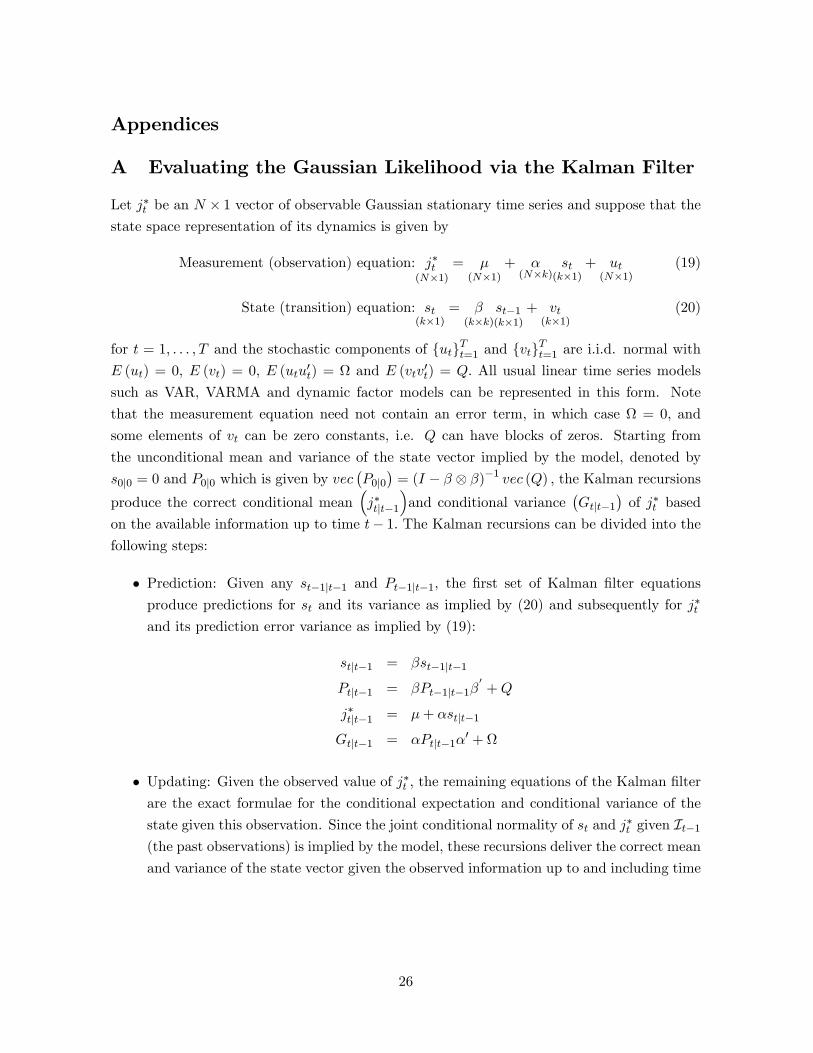
A Evaluating the Gaussian Likelihood via the Kalman Filter
Let j∗t be an N × 1 vector of observable Gaussian stationary time series and suppose that the
state space representation of its dynamics is given by
Measurement (observation) equation: j∗t(N×1)
= µ(N×1)
+ α(N×k)
st(k×1)
+ ut(N×1)
(19)
State (transition) equation: st(k×1)
= β(k×k)
st−1(k×1)
+ vt(k×1)
(20)
for t = 1, . . . , T and the stochastic components of utTt=1 and vtTt=1 are i.i.d. normal with
E (ut) = 0, E (vt) = 0, E (utu′t) = Ω and E (vtv
′t) = Q. All usual linear time series models
such as VAR, VARMA and dynamic factor models can be represented in this form. Note
that the measurement equation need not contain an error term, in which case Ω = 0, and
some elements of vt can be zero constants, i.e. Q can have blocks of zeros. Starting from
the unconditional mean and variance of the state vector implied by the model, denoted by
s0|0 = 0 and P0|0 which is given by vec(P0|0
)= (I − β ⊗ β)−1 vec (Q) , the Kalman recursions
produce the correct conditional mean(j∗t|t−1
)and conditional variance
(Gt|t−1
)of j∗t based
on the available information up to time t− 1. The Kalman recursions can be divided into the
following steps:
• Prediction: Given any st−1|t−1 and Pt−1|t−1, the first set of Kalman filter equations
produce predictions for st and its variance as implied by (20) and subsequently for j∗tand its prediction error variance as implied by (19):
st|t−1 = βst−1|t−1
Pt|t−1 = βPt−1|t−1β′+Q
j∗t|t−1 = µ+ αst|t−1
Gt|t−1 = αPt|t−1α′ + Ω
• Updating: Given the observed value of j∗t , the remaining equations of the Kalman filterare the exact formulae for the conditional expectation and conditional variance of the
state given this observation. Since the joint conditional normality of st and j∗t given It−1
(the past observations) is implied by the model, these recursions deliver the correct mean
and variance of the state vector given the observed information up to and including time
26
t. These are
st|t = st|t−1 + Cov(st, j∗t | It−1)V ar(j∗t | It−1)−1
(j∗t − j∗t|t−1
)= st|t−1 + Pt|t−1α
′G−1t|t−1et|t−1
Pt|t = V ar(st | It−1)− Cov(st, j∗t | It−1)V ar(j∗t | It−1)−1Cov(st, j
∗t | It−1)′
= Pt|t−1 − Pt|t−1α′G−1t|t−1αPt|t−1.
The updating equations can be more succinctly written in terms of the Kalman gain Kt,
which is defined by Kt = Pt|t−1α′G−1t|t−1, to obtain
st|t = st|t−1 +Ktet|t−1
Pt|t = Pt|t−1 −KtGt|t−1K′t.
• By sequential conditioning, the likelihood function can be written as the product ofthe likelihood of each observation given the past, and the Kalman filter recursively
produces all ingredients needed for the calculation of these conditional likelihoods. The
log-likelihood function is then simply computed using
lnL = −NT2
ln (2π)− 1
2
T∑t=1
ln |Gt|t−1| −1
2
T∑t=1
e′t|t−1G
−1t|t−1et|t−1,
and the parameters can be estimated by maximizing this function.
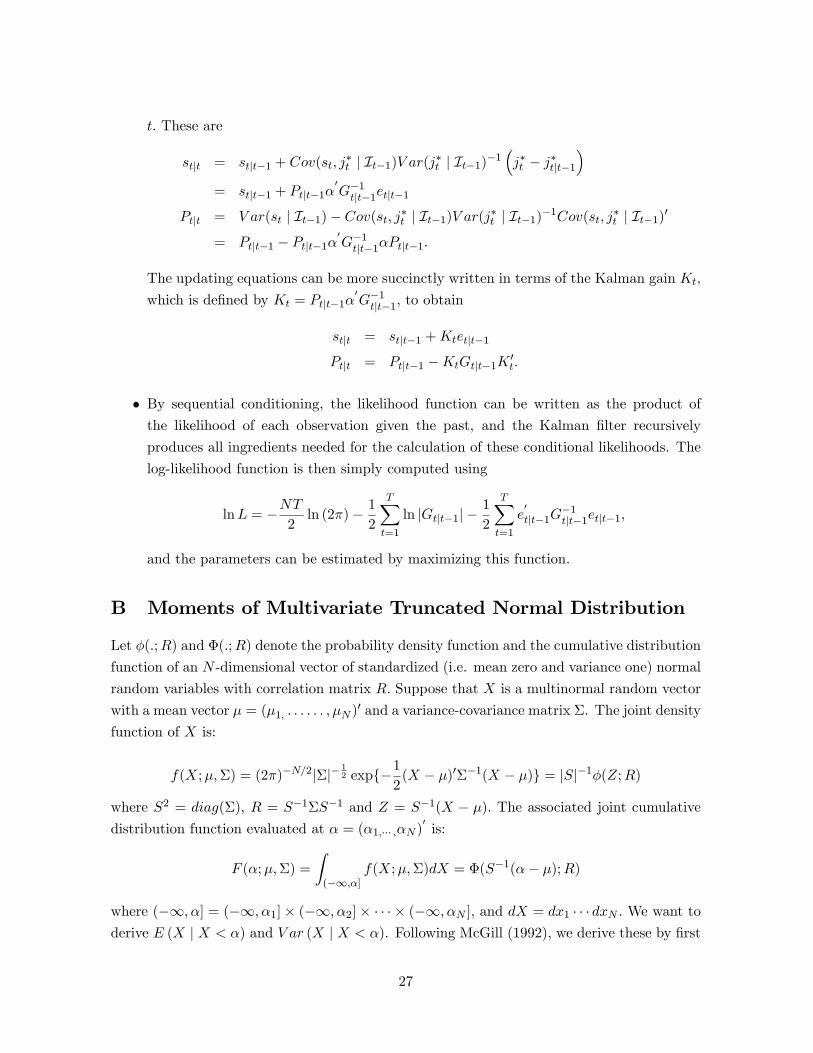
B Moments of Multivariate Truncated Normal Distribution
Let φ(.;R) and Φ(.;R) denote the probability density function and the cumulative distribution
function of an N -dimensional vector of standardized (i.e. mean zero and variance one) normal
random variables with correlation matrix R. Suppose that X is a multinormal random vector
with a mean vector µ = (µ1, . . . . . . , µN )′ and a variance-covariance matrix Σ. The joint density
function of X is:
f(X;µ,Σ) = (2π)−N/2|Σ|−12 exp−1
2(X − µ)′Σ−1(X − µ) = |S|−1φ(Z;R)
where S2 = diag(Σ), R = S−1ΣS−1 and Z = S−1(X − µ). The associated joint cumulative
distribution function evaluated at α = (α1,··· ,αN )′is:
F (α;µ,Σ) =
∫(−∞,α]
f(X;µ,Σ)dX = Φ(S−1(α− µ);R)
where (−∞, α] = (−∞, α1]× (−∞, α2]× · · · × (−∞, αN ], and dX = dx1 · · · dxN . We want toderive E (X | X < α) and V ar (X | X < α). Following McGill (1992), we derive these by first
27
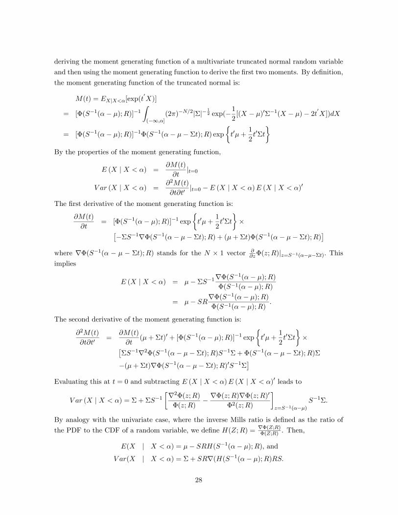
deriving the moment generating function of a multivariate truncated normal random variable
and then using the moment generating function to derive the first two moments. By definition,
the moment generating function of the truncated normal is:
M(t) = EX|X<α[exp(t′X)]
= [Φ(S−1(α− µ);R)]−1
∫(−∞,α]
(2π)−N/2|Σ|−12 exp(−1
2[(X − µ)′Σ−1(X − µ)− 2t
′X])dX
= [Φ(S−1(α− µ);R)]−1Φ(S−1(α− µ− Σt);R) exp
t′µ+
1
2t′Σt
By the properties of the moment generating function,
E (X | X < α) =∂M(t)
∂t|t=0
V ar (X | X < α) =∂2M(t)
∂t∂t′|t=0 − E (X | X < α)E (X | X < α)′
The first derivative of the moment generating function is:
∂M(t)
∂t= [Φ(S−1(α− µ);R)]−1 exp
t′µ+
1
2t′Σt
×[
−ΣS−1∇Φ(S−1(α− µ− Σt);R) + (µ+ Σt)Φ(S−1(α− µ− Σt);R)]
where ∇Φ(S−1(α − µ − Σt);R) stands for the N × 1 vector ∂∂zΦ(z;R)|z=S−1(α−µ−Σt). This
implies
E (X | X < α) = µ− ΣS−1∇Φ(S−1(α− µ);R)
Φ(S−1(α− µ);R)
= µ− SR∇Φ(S−1(α− µ);R)
Φ(S−1(α− µ);R).
The second derivative of the moment generating function is:
∂2M(t)
∂t∂t′=
∂M(t)
∂t(µ+ Σt)′ + [Φ(S−1(α− µ);R)]−1 exp
t′µ+
1
2t′Σt
×[
ΣS−1∇2Φ(S−1(α− µ− Σt);R)S−1Σ + Φ(S−1(α− µ− Σt);R)Σ
−(µ+ Σt)∇Φ(S−1(α− µ− Σt);R)′S−1Σ]
Evaluating this at t = 0 and subtracting E (X | X < α)E (X | X < α)′ leads to
V ar (X | X < α) = Σ + ΣS−1
[∇2Φ(z;R)
Φ(z;R)− ∇Φ(z;R)∇Φ(z;R)′
Φ2(z;R)
]z=S−1(α−µ)
S−1Σ.
By analogy with the univariate case, where the inverse Mills ratio is defined as the ratio of
the PDF to the CDF of a random variable, we define H(Z;R) = ∇Φ(Z;R)Φ(Z;R) . Then,
E(X | X < α) = µ− SRH(S−1(α− µ);R), and
V ar(X | X < α) = Σ + SR∇(H(S−1(α− µ);R)RS.
28
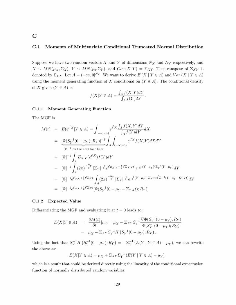
C
C.1 Moments of Multivariate Conditional Truncated Normal Distribution
Suppose we have two random vectors X and Y of dimensions NX and NY respectively, and
X ∼ MN(µX ,ΣX), Y ∼ MN(µY,ΣY ), and Cov (X,Y ) = ΣXY . The transpose of ΣXY is
denoted by ΣY X . Let A = (−∞, 0]NY .We want to derive E (X | Y ∈ A) and V ar (X | Y ∈ A)
using the moment generating function of X conditional on (Y ∈ A) . The conditional density
of X given (Y ∈ A) is:
f(X|Y ∈ A) =
∫A f(X,Y )dY∫A f(Y )dY
.
C.1.1 Moment Generating Function
The MGF is
M(t) = E(et′X |Y ∈ A) =
∫(−∞,∞)
et′X
∫A f(X,Y )dY∫A f(Y )dY
dX
= [Φ(S−1Y (0− µY );RY )]−1︸ ︷︷ ︸
[Φ]−1 on the next four lines
∫A
∫(−∞,∞)
et′Xf(X,Y )dXdY
= [Φ]−1
∫AEX|Y (et
′X)f(Y )dY
= [Φ]−1
∫A
(2π)−NY2 |ΣY |
−12 et
′µX|Y + 12t′ΣX|Y t.e
−12
(Y−µY )′Σ−1Y (Y−µY )dY
= [Φ]−1et′µX+ 1
2t′ΣX t
∫A
(2π)−NY2 |ΣY |
−12 e−12
(Y−µY −ΣYX t)′Σ−1(Y−µY −ΣYX t)dY
= [Φ]−1et′µX+ 1
2t′ΣX t[Φ(S−1
Y (0− µY − ΣY Xt);RY )]
C.1.2 Expected Value
Differentiating the MGF and evaluating it at t = 0 leads to:
E(X|Y ∈ A) =∂M(t)
∂t|t=0 = µX − ΣXY S
−1Y
∇Φ(S−1Y (0− µY );RY )
Φ(S−1Y (0− µY );RY )
= µX − ΣXY S−1Y H
(S−1Y (0− µY );RY
).
Using the fact that S−1Y H
(S−1Y (0− µY );RY
)= −Σ−1
Y (E(Y | Y ∈ A)− µY ), we can rewrite
the above as:
E(X|Y ∈ A) = µX + ΣXY Σ−1Y (E(Y | Y ∈ A)− µY ) ,
which is a result that could be derived directly using the linearity of the conditional expectation
function of normally distributed random variables.
29
C.1.3 Variance
We know that:
V ar(X|Y ∈ A) = E(XX ′|Y ∈ A)− E(X|Y ∈ A)E(X|Y ∈ A)′
=∂2M(t)
∂t∂t′|t=0 − E(X|Y ∈ A)E(X|Y ∈ A)′
and
E(XX ′|Y ∈ A) =∂2M(t)
∂t∂t′|t=0 = ΣX + µXµ
′X −
2µX∇Φ(S−1
Y (0− µY );RY )′
Φ(S−1Y (0− µY );RY )
S−1Y ΣY X + ΣXY S
−1Y [∇2Φ(S−1
Y (0− µY );RY )
Φ(S−1Y (0− µY );RY )
]S−1Y ΣY X .
These lead to
V ar(X|Y ∈ A) = ΣX + ΣXY S−1Y ∇[H(S−1
Y (0− µY );RY ]S−1Y ΣY X .
Since ∇(H(S−1Y (0− µY );RY ) = −(SYRY )−1(ΣY − V ar(Y |Y ∈ A))(RY SY )−1,18 the variance
expression can be transformed to:
V ar(X|Y ∈ A) = ΣX − ΣXY Σ−1Y (ΣY − V ar(Y |Y ∈ A))Σ−1
Y ΣY X
C.2 Moments of Multivariate Conditional Mixed Truncated Normal andNormal Distribution
Suppose we have three normally distributed vectors X, Y and Z of dimensions NX , NY and
NZ , where X ∼MN(µX,ΣX) , Y ∼MN(µY,ΣY ), and Z ∼MN(µZ,ΣZ), and let ΣUV denote
covariance between random vectors U and V with ΣV U = Σ′UV . Let A = (−∞, 0]NY . We want
to derive the E (X|Y ∈ A,Z) and V ar (X|Y ∈ A,Z) using the moment generating function of
X conditional on (Y ∈ A,Z) . The conditional density of X given (Y ∈ A,Z) is:
f(X|Y ∈ A,Z) =
∫A f(X,Y |Z)dY∫A f(Y |Z)dY
.
18See Appendix B for mathematical proof.
30
C.2.1 Moment Generating Function
The MGF is
M(t) = E(et′X |Y ∈ A,Z) =
∫(−∞,∞)
∫(−∞,0] e
t′Xf(X,Y |Z)dY∫
(−∞,0] f(Y |Z)dYdX
= [Φ(S−1Y |Z(0− µY |Z);RY |Z)]−1︸ ︷︷ ︸
[Φ]−1 on the next three lines
∫(−∞,0]
(
∫(−∞,∞)
et′Xf(X|Y,Z)dX).f(Y |Z)dY
= [Φ]−1
∫(−∞,0]
EX|Y,Z(et′X).f(Y |Z)dY
= [Φ]−1 1
|ΣY |Z |(2π)
−NY2
∫(−∞,0]
et′uX|Y,Z+ 1
2t′ΣX|Y,Zt · e
−12
(Y−uY |Z)′Σ−1Y |Z(Y−uY |Z)
dY
= [Φ]−1et′µX|Z+ 1
2t′ΣX|Zt[Φ(S−1
Y |Z(0− µY |Z − ΣXY |Zt);RY |Z)].
C.2.2 Expected Value
By definition:
E(X|Y ∈ A,Z) =∂M(t)
∂t|t=0 = µX|Z − ΣXY |ZS
−1Y |Z
∇Φ(S−1Y |Z(0− µY |Z);RY |Z)
Φ(S−1Y |Z(0− µY |Z);RY |Z)
Since
E(X|Y ∈ A,Z) = µX|Z + ΣXY |ZS−1Y |Z(SY |ZRY |Z)−1(E(Y |Y ∈ A,Z)− µY |Z)
= µX|Z + ΣXY |ZΣ−1Y |Z(E(Y |Y ∈ A,Z)− µY |Z)
= µX + ΣX,(Y,Z)Σ−1(Y,Z)
(E(Y |Y ∈ A,Z)− µY
Z − µZ
)(21)
where ΣX(Y,Z) is the covariance between X and the vector (Y ′, Z ′)′ , Σ(Y,Z) is the variance
matrix of (Y ′, Z ′)′.
C.2.3 Variance
By definition,
E(XX ′|Y ∈ A) =∂2M(t)
∂t∂t′|t=0
= ΣX|Z + µX|Zµ′X|Z − 2µX|Z
∇Φ(S−1Y |Z(0− µY |Z);RY |Z)
Φ(S−1Y |Z(0− µY |Z);RY |Z)
S−1Y |ZΣY X|Z
+ΣXY |ZS−1Y |Z [∇2Φ(S−1
Y |Z(0− µY |Z);RY |Z)
Φ(S−1Y |Z(0− µY |Z);RY |Z)
]S−1Y |ZΣY X|Z .
31
Hence,
V ar(X|Y ∈ A,Z) = E(XX ′|Y ∈ A,Z)− E(X|Y ∈ A,Z)E(X|Y ∈ A,Z)′
= ΣX|Z − ΣXY |ZS−1Y |Z∇H
((S−1Y |Z(0− µY |Z);RY |Z
)S−1Y |ZΣY X|Z
Since
∇H(S−1Y |Z(0− µY |Z);RY |Z
)= (SY |ZRY |Z)−1(ΣY |Z − V ar(Y |Y ∈ A,Z))(RY |ZSY |Z)−1,
the variance expression can be transformed to:
V ar(X|Y ∈ A,Z) = ΣX|Z − ΣXY |ZΣ−1Y |Z(ΣY |Z − V ar(Y |Y ∈ A,Z))Σ−1
Y |ZΣY X|Z
= ΣX − ΣX(Y,Z)Σ−1(Y,Z)Σ
M(Y,Z)Σ
−1(Y,Z)Σ(Y,Z)X (22)
where
ΣM(Y,Z) =
[ΣY − V ar(Y |Y ∈ A,Z) ΣY Z
ΣY Z ΣZ
]. The significance of formulating the condi-
tional mean and variance as in equations (21) and (22) is that it shows that the only differ-
ence between updating the mean and variance of X when both Y and Z are fully observed
and the case where Z is observed but Y is only known to be in A is that the innovation in
Y is E(Y |Y ∈ A,Z) − µY instead of Y − µY and the middle matrix sandwiched between
ΣX(Y,Z)Σ−1(Y,Z) and Σ−1
(Y,Z)Σ(Y,Z)X is ΣM(Y,Z) instead of Σ(Y,Z).
D Realized Volatility, its Components and their Measurement
We assume that the logarithm of the asset price within the active part of the trading day
evolves in continuous time as a standard jump-diffusion process given by
dp(t) = u(t)dt+ σ(t)dw(t) + κ(t)dq(t), (23)
where u(t) denotes the drift term that has continuous and locally bounded variation, σ(t) is a
strictly positive spot volatility process and w(t) is a standard Brownian motion. The κ(t)dq(t)
term refers to a pure jump component, where k(t) is the size of jump and dq(t) = 1 if there
is a jump at time t (and 0 otherwise). The corresponding discrete-time within-day geometric
returns are
rt+j4 = p(t+ j/M)− p(t+ (j − 1)/M), j = 1, 2, ....M, (24)
where M refers to the number of intraday equally spaced returns over the trading day t, and
∆ = 1/M denotes the sampling interval. As such, the daily return for the active part of the
trading day equals rt+1 =∑M
j=1 rt+j4.
32
The quadratic variation of the process in (23) is typically estimated by realized volatility
(RV ), which is defined as the sum of the intraday squared returns, i.e.
RVt+1(∆) ≡M∑j=1
r2t+j∆, (25)
whereas the integrated variance in (23) is typically estimated using realized bi-power variation
defined by
RBVt+1(∆) ≡ π
2(
M
M − 1)M∑j=2
|rt+j∆||rt+(j−1)∆| (26)
(see Andersen and Bollerslev, 1998, Andersen et al., 2003, and Barndorff-Nielsen and Shep-
hard, 2002a,b for further discussion of (3) and Barndorff-Nielsen and Shephard, 2004, 2006
for further discussion of (4)). Given appropriate regularity conditions, the latter papers show
that
plimM→∞
RVt+1(∆) =
∫ t+1
tσ2(s)ds+
∑t<s<t+1
κ2(s) and (27)
plimM→∞
RBVt+1(∆) =
∫ t+1
tσ2(s)ds,
so that the above estimators are consistent estimators for quadratic variation and integrated
variance respectively. This motivated Barndorff-Nielsen and Shephard (2004) and Andersen
et al. (2007) to suggest the use of
Jt+1(∆) = maxRVt+1(∆)−RBVt+1(∆), 0 (28)
as a consistent measure of the jump contribution to realized volatility, where the truncation
at zero ensures that all daily measures of this contribution are non-negative. The continuous
component is then measured by
Ct+1(∆) = minRVt+1(∆), RBVt+1(∆) (29)
to ensure that the continuous and jump components add to realized volatility.
In practice, the measurement of realized volatility and its components is often complicated
by microstructure issues. When microstructure noise is present, equations (25) and (26)
provide biased estimates of the quadratic variation and integrated volatility associated with
the fundamental price. Further, the finite size of the sampling interval (∆) allows additional
contamination to affect estimates of integrated volatility based on (26). See Zhang et al.
(2005), Huang and Tauchen (2005) and Andersen et al. (2011) for detailed discussion on the
effects of (i.i.d.) microstructure noise, and Andersen et al. (2010) and Corsi et al. (2010)
for discussion on finite sampling size effects. Many authors including those mentioned here
have suggested alternative estimators of integrated quarticity and integrated variance that can
improve estimation, depending on the data at hand and the purpose of estimation.
33
References
Ahn, S. K. and G. C. Reinsel (1988). Nested reduced-rank autoregressive models for multiple
time series. Journal of the American Statistical Association 83, 849—856.
Ait-Sahalia, Y., P. A. Mykland, and L. Zhang (2005). How often to sample a continuous-time
process in the presence of market microstructure noise. Review of Financial Studies 18,
351—416.
Andersen, T. G., L. Benzoni, and J. Lund (2002). An empirical investigation of continuous-
time equity return models. Journal of Finance 57 (3), 1239—1284.
Andersen, T. G. and T. Bollerslev (1998). Answering the skeptics: Yes, standard volatility
models do provide accurate forecasts. International Economic Review 39, 885—905.
Andersen, T. G., T. Bollerslev, and F. X. Diebold (2007). Roughing it up: Including jump
components in measuring, modeling and forecasting return volatility. The Review of Eco-
nomics and Statistics 89, 701—720.
Andersen, T. G., T. Bollerslev, F. X. Diebold, and P. Labys (2000). Great realizations. Risk 13,
105—108.
Andersen, T. G., T. Bollerslev, F. X. Diebold, and P. Labys (2003). Modeling and forecasting
realized volatility. Econometrica 71, 579—625.
Andersen, T. G., T. Bollerslev, and X. Huang (2011). A reduced form framework for modeling
volatility of speculative prices based on realized variation measures. Journal of Economet-
rics 160, 176—189.
Andersen, T. G., D. Dobrev, and E. Schaumburg (2010). Jump-robust volatility estimation
using nearest neighbor truncation. Federal Reserve Bank of New York, Staff Reports.
Anderson, H. M. and F. Vahid (2007). Forecasting the volatility of Australian stock returns:
Do common factors help? Journal of Business and Economic Statistics 25, 76—90.
Angelidis, T. and S. Degiannakis (2007). Backtesting VaR models: A two-stage procedure.
The Journal of Risk Model Validation 1, 27—48.
Bandi, F. and J. R. Russell (2008). Microstructure noise, realized volatility, and optimal
sampling. The Review of Economics Studies 75, 339—369.
Barndorff-Nielsen, O. E. and N. Shephard (2002a). Econometric analysis of realized volatil-
ity and its use in estimating stochastic volatility models. Journal of the Royal Statistical
Society 64, 253—280.
34
Barndorff-Nielsen, O. E. and N. Shephard (2002b). Estimating quadratic variation using
realized variance. Journal of Applied Econometrics 17, 457—478.
Barndorff-Nielsen, O. E. and N. Shephard (2004). Power and bipower variation with stochastic
volatility and jumps. Journal of Financial Econometrics 2, 1—37.
Barndorff-Nielsen, O. E. and N. Shephard (2006). Econometrics of testing for jumps in financial
economics using bipower variation. Journal of Financial Econometrics 4, 1—30.
Bollerslev, T., T. H. Law, and G. Tauchen (2008). Risk, jumps and diversification. Journal
of Econometrics 144, 234—256.
Brockwell, P. J. and R. A. Davis (1991). Time Series: Theory and Methods (Second ed.).
Springer.
Busch, T., B. J. Christensen, and M. O. Nielsen (2011). The role of implied volatility in
forecasting future realized volatility and jumps in foreign exchange, stock, and bond markets.
Journal of Econometrics 160 (1), 48—57.
Christoffersen, P. (1998). Evaluating interval forecasts. International Economic Review 39,
841—862.
Corsi, F. (2009). A simple approximate long-memory model of realized volatility. Journal of
Financial Econometrics 7, 174—196.
Corsi, F., D. R. Pirino, and R. Reno (2010). Threshold bipower variation and the impact of
jumps on volatility forecasting. Journal of Econometrics 159, 276—288.
Diebold, F. X. and R. S. Mariano (1995). Comparing predictive accuracy. Journal of Business
and Economic Statistics 13, 253—263.
Engle, R. and M. W. Watson (1981). A one-factor multivariate time series model of metropol-
itan wage rates. Journal of the American Statistical Association 76, 774—781.
Eraker, B., M. Johannes, and N. Polson (2003). The impact of jumps in volatility and returns.
Journal of Finance 58 (3), 1269—1300.
Geweke, J. (1977). The dynamic factor analysis of economic time-series models. In D. J. Aigner
and A. S. Goldberger (Eds.), Latent Variables in Socio-Economic Models. North-Holland.
Hamilton, J. D. (1994). Time Series Analysis. Princeton University Press.
Hansen, P. R. and A. Lunde (2006). Realized variance and market microstructure noise.
Journal of Business and Economic Statistics 24 (2), 127—161.
35
Harvey, A. C., E. Ruiz, and E. Sentana (1992). Unobserved component time series models
with ARCH disturbances. Journal of Econometrics 52, 129—157.
Huang, X. and G. Tauchen (2005). The relative contribution of jumps to total price variance.
Journal of Financial Econometrics 3, 456—499.
Jacod, J. and V. Todorov (2009). Testing for common arrivals of jumps for discretely observed
multi-dimentional process. Annuals of Statistics 37, 1792—1838.
Kupiec, P. H. (1995). Techniques for verifying the accuracy of risk measurement models. The
Journal of Derivatives 3, 73—84.
Lanne, M. (2007). Forecasting realized exchange rate volatility by decomposition. Interna-
tional Journal of Forecasting 23, 307—320.
Lee, L. F. (1999). Estimation of dynamic and ARCH Tobit models. Journal of Economet-
rics 92, 355—390.
Liao, Y. (2011). Does Decomposing Realized Volatility Help in Risk Prediction: Evidence
from the Chinese Mainland Stock Market. Ph. D. thesis, Research School of Economics,
Australian National University.
Liao, Y. and H. M. Anderson (2011). Testing for co-jumps in high-frequency financial data:
An approach based on first-high-low-last prices. Monash University Working Paper No.
9/11 .
Lütkepohl, H. (1993). Introduction to Multiple Time Series Analysis (2nd ed.). Springer-
Verlag, Berlin-Heidelberg.
Ma, C. and X. Wang (2009). The jump behavior of China’s stock market prices: A non-
parametric analysis with the high frequency data of the SSE composite index. Working
paper, Xiamen University, 2009.
Marcucci, J. (2008). Are common factors useful in forecasting international stock market real-
ized variances? "Factor Structures for Panel and Multivariate Time Series Data" Conference
paper, 2008.
McGill, J. I. (1992). The multivariate hazard gradient and moments of the truncated multi-
normal distribution. Communications in Statistics—Theory and Methods 21, 3053—3060.
Merton, R. C. (1976). Option pricing when underlying stock returns are continuous. Journal
of Financial Economics 3, 125—144.
Schwarz, G. (1978). Estimating the dimension of a model. Annals of Statistics 6 (2), 461—464.
36

Tobin, J. (1958). Estimation of relationships for limited dependent variables. Econometrica 26,
24—36.
Vahid, F. and J. V. Issler (2002). The importance of common cyclical features in VAR analysis:
A Monte-Carlo study. Journal of Econometrics 109, 341—363.
Velu, R., G. Reinsel, and D. Wickern (1986). Reduced rank models for multiple time series.
Biometrika 73, 105—118.
Wang, C. F., N. Yao, Z. M. Fang, and Y. Li (2008). An empirical research on jump behavior
of realized volatility in Chinese stock markets. System Engineering 26.
Xu, Z. G. and S. Y. Zhang (2006). Research on the modelling of realized volatility based on
multivariate high-frequency data. Journal of System Engineering 21.
Zeger, S. L. and R. Brookmeyer (1986). Regression analysis with censored autocorrelated
data. Journal of the American Statistical Association 81, 722—729.
Zhang, L., P. A. Mykland, and Y. Ait-Sahalia (2005). A tale of two time scales: Determining
integrated volatility with noisy high-frequency data. Journal of the American Statistical
Association 100, 1394—1411.
37
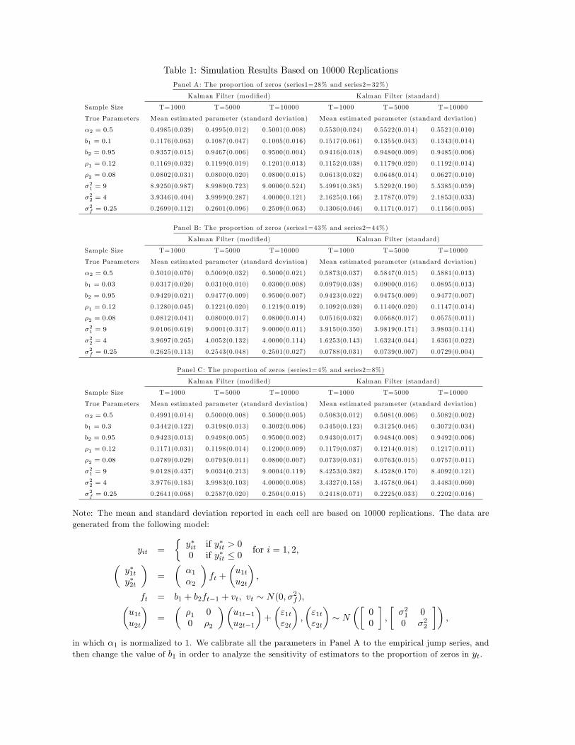
Table 1: Simulation Results Based on 10000 Replications
Panel A: The proportion of zeros (series1=28% and series2=32%)
Kalman Filter (modied) Kalman Filter (standard)
Sample Size T=1000 T=5000 T=10000 T=1000 T=5000 T=10000
True Parameters Mean estimated parameter (standard deviation) Mean estimated parameter (standard deviation)
2 = 0:5 0.4985(0.039) 0.4995(0.012) 0.5001(0.008) 0.5530(0.024) 0.5522(0.014) 0.5521(0.010)
b1 = 0:1 0.1176(0.063) 0.1087(0.047) 0.1005(0.016) 0.1517(0.061) 0.1355(0.043) 0.1343(0.014)
b2 = 0:95 0.9357(0.015) 0.9467(0.006) 0.9500(0.004) 0.9416(0.018) 0.9480(0.009) 0.9485(0.006)
1 = 0:12 0.1169(0.032) 0.1199(0.019) 0.1201(0.013) 0.1152(0.038) 0.1179(0.020) 0.1192(0.014)
2 = 0:08 0.0802(0.031) 0.0800(0.020) 0.0800(0.015) 0.0613(0.032) 0.0648(0.014) 0.0627(0.010)
21 = 9 8.9250(0.987) 8.9989(0.723) 9.0000(0.524) 5.4991(0.385) 5.5292(0.190) 5.5385(0.059)
22 = 4 3.9346(0.404) 3.9999(0.287) 4.0000(0.121) 2.1625(0.166) 2.1787(0.079) 2.1853(0.033)
2f = 0:25 0.2699(0.112) 0.2601(0.096) 0.2509(0.063) 0.1306(0.046) 0.1171(0.017) 0.1156(0.005)
Panel B: The proportion of zeros (series1=43% and series2=44%)
Kalman Filter (modied) Kalman Filter (standard)
Sample Size T=1000 T=5000 T=10000 T=1000 T=5000 T=10000
True Parameters Mean estimated parameter (standard deviation) Mean estimated parameter (standard deviation)
2 = 0:5 0.5010(0.070) 0.5009(0.032) 0.5000(0.021) 0.5873(0.037) 0.5847(0.015) 0.5881(0.013)
b1 = 0:03 0.0317(0.020) 0.0310(0.010) 0.0300(0.008) 0.0979(0.038) 0.0900(0.016) 0.0895(0.013)
b2 = 0:95 0.9429(0.021) 0.9477(0.009) 0.9500(0.007) 0.9423(0.022) 0.9475(0.009) 0.9477(0.007)
1 = 0:12 0.1280(0.045) 0.1221(0.020) 0.1219(0.019) 0.1092(0.039) 0.1140(0.020) 0.1147(0.014)
2 = 0:08 0.0812(0.041) 0.0800(0.017) 0.0800(0.014) 0.0516(0.032) 0.0568(0.017) 0.0575(0.011)
21 = 9 9.0106(0.619) 9.0001(0.317) 9.0000(0.011) 3.9150(0.350) 3.9819(0.171) 3.9803(0.114)
22 = 4 3.9697(0.265) 4.0052(0.132) 4.0000(0.114) 1.6253(0.143) 1.6324(0.044) 1.6361(0.022)
2f = 0:25 0.2625(0.113) 0.2543(0.048) 0.2501(0.027) 0.0788(0.031) 0.0739(0.007) 0.0729(0.004)
Panel C: The proportion of zeros (series1=4% and series2=8%)
Kalman Filter (modied) Kalman Filter (standard)
Sample Size T=1000 T=5000 T=10000 T=1000 T=5000 T=10000
True Parameters Mean estimated parameter (standard deviation) Mean estimated parameter (standard deviation)
2 = 0:5 0.4991(0.014) 0.5000(0.008) 0.5000(0.005) 0.5083(0.012) 0.5081(0.006) 0.5082(0.002)
b1 = 0:3 0.3442(0.122) 0.3198(0.013) 0.3002(0.006) 0.3450(0.123) 0.3125(0.046) 0.3072(0.034)
b2 = 0:95 0.9423(0.013) 0.9498(0.005) 0.9500(0.002) 0.9430(0.017) 0.9484(0.008) 0.9492(0.006)
1 = 0:12 0.1171(0.031) 0.1198(0.014) 0.1200(0.009) 0.1179(0.037) 0.1214(0.018) 0.1217(0.011)
2 = 0:08 0.0789(0.029) 0.0793(0.011) 0.0800(0.007) 0.0739(0.031) 0.0763(0.015) 0.0757(0.011)
21 = 9 9.0128(0.437) 9.0034(0.213) 9.0004(0.119) 8.4253(0.382) 8.4528(0.170) 8.4092(0.121)
22 = 4 3.9776(0.183) 3.9983(0.103) 4.0000(0.008) 3.4327(0.158) 3.4578(0.064) 3.4483(0.060)
2f = 0:25 0.2641(0.068) 0.2587(0.020) 0.2504(0.015) 0.2418(0.071) 0.2225(0.033) 0.2202(0.016)
Note: The mean and standard deviation reported in each cell are based on 10000 replications. The data aregenerated from the following model:
yit =
yit if yit > 00 if yit 0
for i = 1; 2;y1ty2t
=
12
ft +
u1tu2t
;
ft = b1 + b2ft1 + vt; vt N(0; 2f );u1tu2t
=
1 00 2
u1t1u2t1
+
"1t"2t
;
"1t"2t
N
00
;
21 00 22
;
in which 1 is normalized to 1. We calibrate all the parameters in Panel A to the empirical jump series, andthen change the value of b1 in order to analyze the sensitivity of estimators to the proportion of zeros in yt.
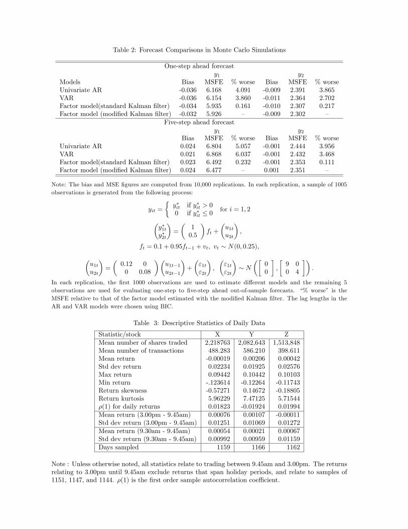
Table 2: Forecast Comparisons in Monte Carlo Simulations
One-step ahead forecasty1 y2
Models Bias MSFE % worse Bias MSFE % worseUnivariate AR -0.036 6.168 4.091 -0.009 2.391 3.865VAR -0.036 6.154 3.860 -0.011 2.364 2.702Factor model(standard Kalman lter) -0.034 5.935 0.161 -0.010 2.307 0.217Factor model (modied Kalman lter) -0.032 5.926 -0.009 2.302
Five-step ahead forecasty1 y2
Bias MSFE % worse Bias MSFE % worseUnivariate AR 0.024 6.804 5.057 -0.001 2.444 3.956VAR 0.021 6.868 6.037 -0.001 2.432 3.468Factor model(standard Kalman lter) 0.023 6.492 0.232 -0.001 2.353 0.111Factor model (modied Kalman lter) 0.024 6.477 0.001 2.351
Note: The bias and MSE gures are computed from 10,000 replications. In each replication, a sample of 1005observations is generated from the following process:
yit =
yit if yit > 00 if yit 0
for i = 1; 2
y1ty2t
=
10:5
ft +
u1tu2t
;
ft = 0:1 + 0:95ft1 + vt; vt N(0; 0:25);u1tu2t
=
0:12 00 0:08
u1t1u2t1
+
"1t"2t
;
"1t"2t
N
00
;
9 00 4
:
In each replication, the rst 1000 observations are used to estimate di¤erent models and the remaining 5observations are used for evaluating one-step to ve-step ahead out-of-sample forecasts. % worse is theMSFE relative to that of the factor model estimated with the modied Kalman lter. The lag lengths in theAR and VAR models were chosen using BIC.
Table 3: Descriptive Statistics of Daily Data
Statistic/stock X Y ZMean number of shares traded 2,218763 2,082,643 1,513,848Mean number of transactions 488.283 586.210 398.611Mean return -0.00019 0.00206 0.00042Std dev return 0.02234 0.01925 0.02576Max return 0.09442 0.10442 0.10103Min return -.123614 -0.12264 -0.11743Return skewness -0.57271 0.14672 -0.18805Return kurtosis 5.96229 7.47125 5.71544(1) for daily returns 0.01823 -0.01924 0.01994Mean return (3.00pm - 9.45am) 0.00076 0.00107 -0.00011Std dev return (3.00pm - 9.45am) 0.01251 0.01069 0.01272Mean return (9.30am - 9.45am) 0.00054 0.00021 0.00067Std dev return (9.30am - 9.45am) 0.00992 0.00959 0.01159Days sampled 1159 1166 1162
Note : Unless otherwise noted, all statistics relate to trading between 9.45am and 3.00pm. The returnsrelating to 3.00pm until 9.45am exclude returns that span holiday periods, and relate to samples of1151, 1147, and 1144. (1) is the rst order sample autocorrelation coe¢ cient.
Table 4: Descriptive Statistics Relating to Microstructure
Statistic/Stock X Y ZMean transactions/min 2.2195 2.6663 1.8118(1) transactions returns -0.3351 -0.5314 -0.3901(1) 1 min returns -0.0269 -0.0574 -0.0882(1) 2 min returns 0.0095 -0.0017 -0.0593(1) 5 min returns -0.1175 -0.0682 -0.1063% zero transaction returns 54.65 51.03 54.12% zero 1 min returns 64.10 57.26 63.50% zero 5 min returns 32.66 27.41 31.28% 1 min obs with no trade 34.68 29.60 33.97% 5 min obs with no trade 9.11 8.11 9.11
Note: (1) is the rst order sample autocorrelation coe¢ cient.
Table 5: Descriptive Statistics Relating to Volatility Components
Decomposition A Decomposition B Some US StocksStatistic/Stock X Y Z X Y Z BA Citi IBMMean RV .00073 .00051 .00099 .00067 .00047 .00090 .00024 .00023 .00010Std Dev RV .00076 .00065 .00099 .00007 .00059 .00088 .00247 .00015 .00008Mean C .00051 .00038 .00072 .00041 .00033 .00064 .00014 .00011 .00008Std Dev C .00060 .00056 .00080 .00044 .00050 .00071 .00030 .00013 .00007Mean J .00022 .00013 .00027 .00026 .00013 .00027 .00008 .00011 .00001Std Dev J .00033 .00021 .00042 .00042 .00021 .00045 .00232 .00006 .00002p-val LB(10) J .0000 .0000 .0000 .0000 .0000 .0000 1.0000 .1350 0.0320p-val LB(20) J .0000 .0000 .0000 .0000 .0000 .0000 1.0000 .5100 0.0000% of zeros in J 11.8 10.3 9.5 20.2 18.0 18.2 26.8 26.3 27.8Days sampled 1159 1166 1162 1159 1166 1162 1256 1253 1250
BA, Citi and IBM denote Boeing Company, Citigroup, and International Business Machines. The US data isfrom the Wharton data base, relates to 2003 - 2007, and measures of RV, C, and J are based on ve minutesampling from 9.30am to 16.00pm. Statistics reported for the US stocks are directly comparable with thosereported for Decomposition A.LB(10) and LB(20) are Ljung-Box tests of the null hypothesis of no serial correlation (against alternatives ofup to 10th or up to 20th order serial correlation).
Table 6a: HAR and HARCJ One-step Ahead Forecasting Models
HAR HARCJCoef X Y Z X Y Z0 -2.261(0.465) -2.059(0.434) -1.177(0.318) -4.547(0.583) -3.927(0.468) -2.623(0.378)D 0.245(0.058) 0.222(0.044) 0.128(0.044)W 0.223(0.080) 0.320(0.078) 0.536(0.078)M 0.254(0.090) 0.222(0.069) 0.192(0.070)CD 0.123(0.041) 0.081(0.034) 0.033(0.033)CW 0.196(0.067) 0.277(0.071) 0.378(0.070)CM 0.110(0.087) 0.167(0.073) 0.232(0.075)JD 0.033(0.087) 0.040(0.016) 0.013(0.006)JW 0.012(0.019) 0.041(0.045) 0.043(0.016)JM 0.079(0.023) 0.078(0.055) 0.010(0.014)R2 0.206 0.249 0.388 0.194 0.222 0.371
R2
0.203 0.246 0.386 0.188 0.218 0.367RMSE 0.502 0.342 0.678 0.508 0.345 0.6972(RV; dRV ) 0.163 0.203 0.271 0.133 0.184 0.221
Table 6b: HAR and HARCJ Five-step Ahead Forecasting Models
HAR HARCJCoef X Y Z X Y Z0 -3.772(0.703) -3.965(0.672) -2.122(0.523) -5.935(0.834) -4.969(0.606) -3.326(0.550)D 0.040(0.045) 0.073(0.048) 0.090(0.045)W 0.187(0.111) 0.270(0.112) 0.348(0.114)M 0.301(0.135) 0.190(0.118) 0.290(0.132)CD 0.039(0.039) 0.022(0.030) 0.041(0.036)CW 0.042(0.099) 0.241(0.096) 0.303(0.109)CM 0.178(0.120) 0.131(0.107) 0.204(0.115)JD -0.024(0.010) 0.009(0.019) 0.003(0.006)JW 0.053(0.021) 0.038(0.517) 0.021(0.021)JM 0.083(0.031) 0.032(0.063) 0.031(0.025)R2 0.083 0.108 0.261 0.095 0.109 0.259
R2
0.080 0.105 0.258 0.089 0.103 0.254RMSE 0.532 0.367 0.734 0.527 0.366 0.7382(RV; dRV ) 0.068 0.089 0.150 0.082 0.090 0.138
The regressions are ln (RV t+1) = 0+D ln (RV t1;t) + W ln (RV t5;t) + M ln (RV t22;t) + "t+1 forHAR and ln (RV t+1) = 0+CD ln (Ct) + CW ln (Ct5;t) + CM ln (Ct22;t) + JD ln (J t+1)+
JW ln (J t5;t+1) + JM ln (J t22;t+1) + "t+1 for HARCJ, whereRV t;t+h= h1[RV t+1+RV t+2+:::::+RV t+h];
Ct;t+h= h1[Ct+1+Ct+2+:::::+ Ct+h] and J t;t+h= h
1[J t+1+J t+2+:::::+ J t+h] for h = 5 and h = 22:The variable ln (J t+1) has been scaled by 10000. We report HAC standard errors in parentheses. The e¤ectivesample size is 853 observations for one-step ahead models and 849 observations for ve-step ahead models. Thesecond last line reports the root mean squared error associated with predicting the levels of RV (scaled by10000) and the last line reports the squared correlation between the levels of RV and predicted levels of RV.
Table 7: Estimated Factor Models
Parameters RV C J J1 -7.774 (0.097) -8.419 (0.131) 3.805 (0.855) 2.263 (0.379)2 -8.292(0.097) -8.976(0.170) 1.965(0.371) 1.251(0.165)3 -7.468(0.140) -8.048(0.191) 4.492(0.932) 2.726(0.439)1 0.114(0.016) 0.125(0.019) 0.527(0.135) 0.431(0.159)2 0.111(0.017) 0.163(0.024) 0.223(0.059) 0.183(0.056)3 0.174(0.022) 0.191(0.027) 0.560(0.148) 0.501(0.280)b1 0.958(0.013) 0.966(0.012) 0.966(0.017) 0.960(0.021)1 0.228(0.042) 0.259(0.048) 0.022(0.043) 0.018(0.043)2 0.299(0.036) 0.212(0.050) 0.097(0.045) 0.091(0.059)3 0.038(0.055) 0.050(0.067) 0.106(0.046) 0.076(0.095)21 0.507(0.035) 0.908(0.062) 13.355(2.055) 10.397(1.453)22 0.508(0.029) 1.181(0.086) 3.613(0.608) 2.791(0.420)23 0.334(0.024) 0.661(0.056) 21.017(3.773) 16.629(2.601)LL -2788.54 3684.7917 -4693.26 6502.40
Measures of in-sample tCorrelation/SSP Model SSP(RV) SSP(C+J) SSP(C+J)RMSE(dRV (Xt+1) 0.506 0.487 0.497RMSE(dRV (Yt+1) 0.348 0.344 0.349RMSE(dRV (Zt+1) 0.667 0.664 0.6722(RV (Xt+1);dRV (Xt+1)) 0.139 0.155 0.1532(RV (Yt+1);dRV (Yt+1)) 0.172 0.158 0.1592(RV (Zt+1);dRV (Zt+1)) 0.296 0.284 0.289
Note : The table reports estimated coe¢ cients for the state space models of realized volatility, the continuouscomponent and jumps, when the variance of the innovation to the factor has been normalized at one. Thejump variables have been transformed to 10000*ln(jumps+1), and the column marked J reports estimates forthe dynamic Tobit factor model while the column marked Jreports estimates when the zeros are not treatedas censored variables. The numbers in parentheses report (quasi-maximum likelihood) standard errors of theparameter estimates. The e¤ective sample size is 874 observations. The reported root mean squared errorsrelate to predicting the levels of RV and they have been scaled by 10000, and the reported squared correlationsrelate to correlations between the levels of RV and predicted levels of RV.
Table 8a: Out-of-sample Forecast Performance: RMSE for 1-step Ahead Forecasts of RV
Stock/Model HAR HARCJ SSP(RV) SSP(C+J) SSP(C+J)X 0.978 1.280 0.961 0.938b 0.931a;b
Y 0.874 0.909 0.936 0.932 0.927a;b
Z 1.124 1.141 1.084 1.077 1.079
Table 8b: Out-of-sample Forecast Performance: RMSE for 5-step Ahead Forecasts of RV
Stock/Model HAR HARCJ SSP(RV) SSP(C+J) SSP(C+J)X 1.108 1.119 1.106 1.084b 1.072a;b
Y 1.037 1.027 1.091 1.057b 1.045a;b
Z 1.245 1.237 1.241 1.218b 1.210
The out-of sample forecast comparison is based on 228 observations from 01/04/2007 to 12/27/2007. Thedash on the J indicates that zeros in the jump series have been treated as actual observations, whereas the Jindicates that zeros have been treated as censored observations. All gures in the table have been multipliedby 104: The superscript indicates that Diebold-Mariano (1995) tests of the null that forecasts are equal isrejected at the 5% level of signicance. The alternatives are : a) RMSE( SSP(C+J))<RMSE(SSP(C+J); andb) RMSE(factor model that treats C and J separately) < RMSE(SSP(RV)).
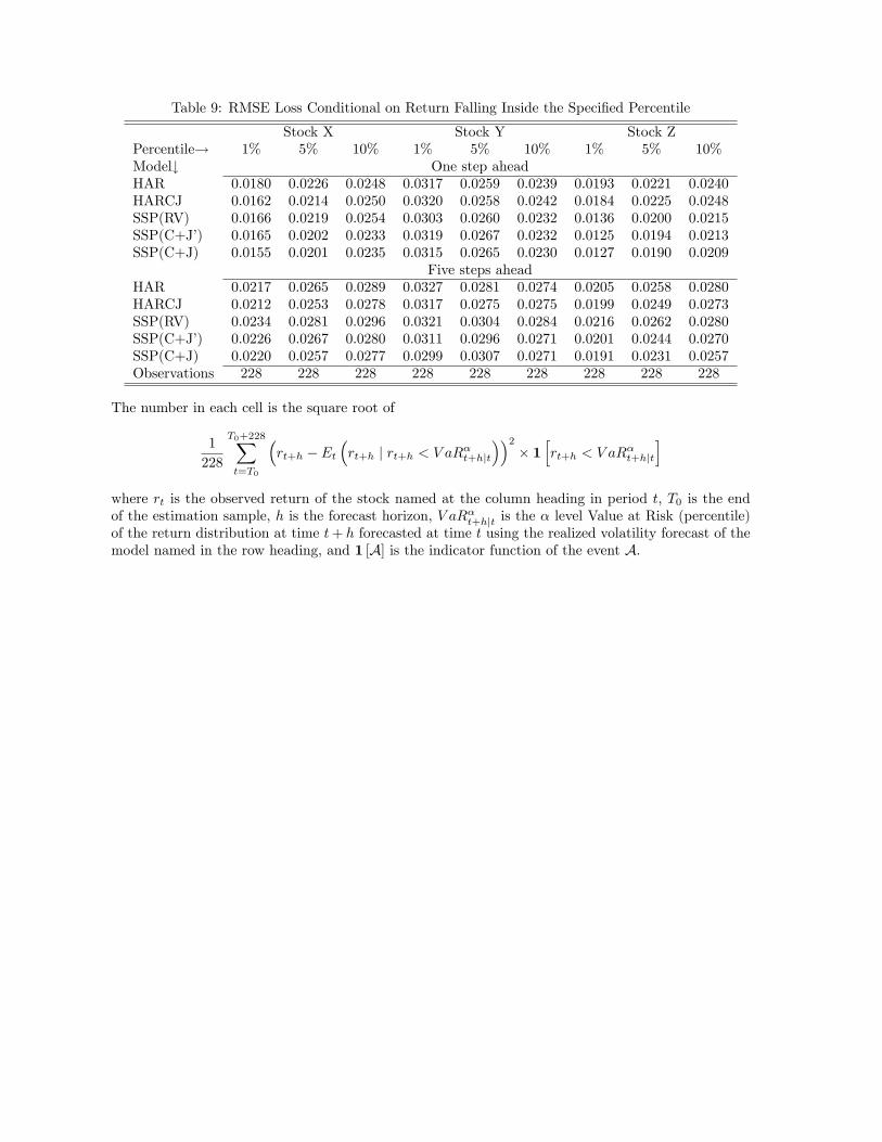
Table 9: RMSE Loss Conditional on Return Falling Inside the Specied Percentile
Stock X Stock Y Stock ZPercentile! 1% 5% 10% 1% 5% 10% 1% 5% 10%Model# One step aheadHAR 0:0180 0:0226 0:0248 0:0317 0:0259 0:0239 0:0193 0:0221 0:0240HARCJ 0:0162 0:0214 0:0250 0:0320 0:0258 0:0242 0:0184 0:0225 0:0248SSP(RV) 0:0166 0:0219 0:0254 0:0303 0:0260 0:0232 0:0136 0:0200 0:0215SSP(C+J) 0:0165 0:0202 0:0233 0:0319 0:0267 0:0232 0:0125 0:0194 0:0213SSP(C+J) 0:0155 0:0201 0:0235 0:0315 0:0265 0:0230 0:0127 0:0190 0:0209
Five steps aheadHAR 0:0217 0:0265 0:0289 0:0327 0:0281 0:0274 0:0205 0:0258 0:0280HARCJ 0:0212 0:0253 0:0278 0:0317 0:0275 0:0275 0:0199 0:0249 0:0273SSP(RV) 0:0234 0:0281 0:0296 0:0321 0:0304 0:0284 0:0216 0:0262 0:0280SSP(C+J) 0:0226 0:0267 0:0280 0:0311 0:0296 0:0271 0:0201 0:0244 0:0270SSP(C+J) 0:0220 0:0257 0:0277 0:0299 0:0307 0:0271 0:0191 0:0231 0:0257Observations 228 228 228 228 228 228 228 228 228
The number in each cell is the square root of
1
228
T0+228Xt=T0
rt+h Et
rt+h j rt+h < V aRt+hjt
2 1
hrt+h < V aR
t+hjt
iwhere rt is the observed return of the stock named at the column heading in period t; T0 is the endof the estimation sample, h is the forecast horizon, V aRt+hjt is the level Value at Risk (percentile)of the return distribution at time t+ h forecasted at time t using the realized volatility forecast of themodel named in the row heading, and 1 [A] is the indicator function of the event A.
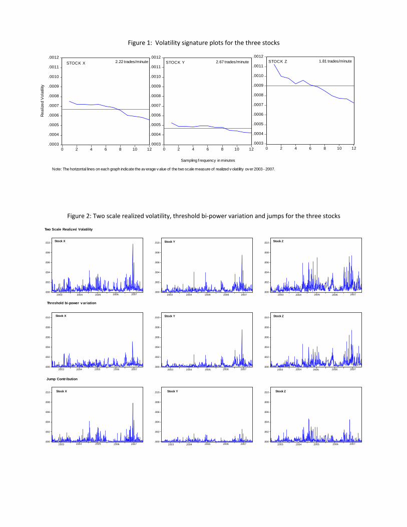
Figure 1: Volatility signature plots for the three stocks
.0003
.0004
.0005
.0006
.0007
.0008
.0009
.0010
.0011
.0012
0 2 4 6 8 10 12.0003
.0004
.0005
.0006
.0007
.0008
.0009
.0010
.0011
.0012
0 2 4 6 8 10 12.0003
.0004
.0005
.0006
.0007
.0008
.0009
.0010
.0011
.0012
0 2 4 6 8 10 12
2.22 trades/minute 2.67 trades/minute 1.81 trades/minuteSTOCK X STOCK Y STOCK Z
Sampling f requency in minutes
Rea
lized
Vol
atili
ty
Note: The horizontal lines on each graph indicate the av erage v alue of the two scale measure of realized v olatility ov er 2003 - 2007.
Figure 2: Two scale realized volatility, threshold bi‐power variation and jumps for the three stocks
.000
.002
.004
.006
.008
.010
2003 2004 2005 2006 2007.000
.002
.004
.006
.008
.010
2003 2004 2005 2006 2007
Stock Y
.000
.002
.004
.006
.008
.010
2003 2004 2005 2006 2007
Stock Z
.000
.002
.004
.006
.008
.010
2003 2004 2005 2006 2007
Stock X
.000
.002
.004
.006
.008
.010
2003 2004 2005 2006 2007
Stock Y
.000
.002
.004
.006
.008
.010 Stock Z
2003 2004 2005 2006 2007
.000
.002
.004
.006
.008
.010
2003 2004 2005 2006 2007
Stock X
.000
.002
.004
.006
.008
.010
2003 2004 2005 2006 2007
Stock Y
.000
.002
.004
.006
.008
.010 Stock Z
2003 2004 2005 2006 2007
Stock X
Two Scale Realized Volatility
Threshold bi-power v ariation
Jump Contribution