Embed Size (px)
Citation preview
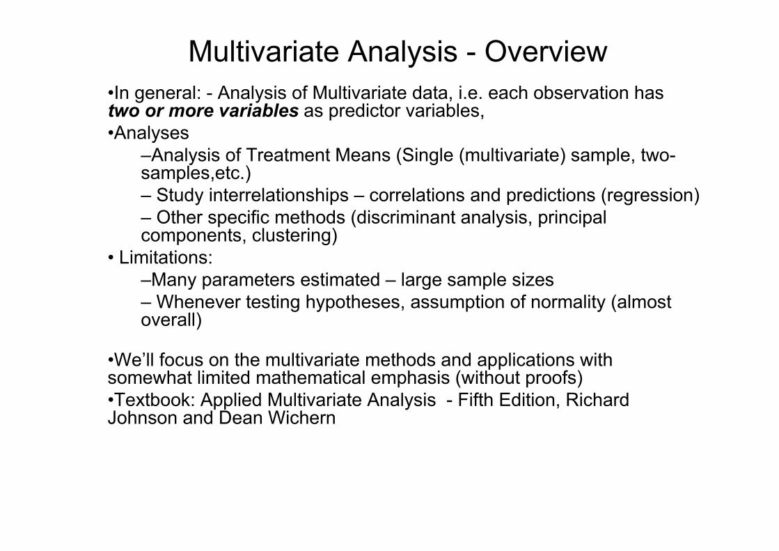
Multivariate Analysis - Overview
•In general: - Analysis of Multivariate data, i.e. each observation has two or more variables as predictor variables,
•Analyses
–Analysis of Treatment Means (Single (multivariate) sample, two-samples,etc.)
– Study interrelationships – correlations and predictions (regression)
– Other specific methods (discriminant analysis, principal components, clustering)
• Limitations:
–Many parameters estimated – large sample sizes
– Whenever testing hypotheses, assumption of normality (almost overall)
•We’ll focus on the multivariate methods and applications with somewhat limited mathematical emphasis (without proofs)
•Textbook: Applied Multivariate Analysis - Fifth Edition, Richard Johnson and Dean Wichern
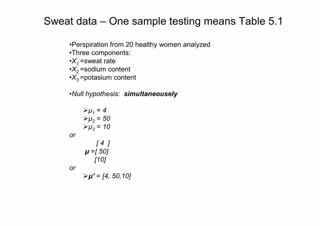
Sweat data – One sample testing means Table 5.1
•Perspiration from 20 healthy women analyzed
•Three components:
•X1 =sweat rate
•X2 =sodium content
•X3 =potasium content
•Null hypothesis: simultaneousely
�µ1 = 4
�µ2 = 50
�µ3 = 10
or
[ 4 ]
µ =[ 50]
[10]
or
�µ’ = [4, 50,10]
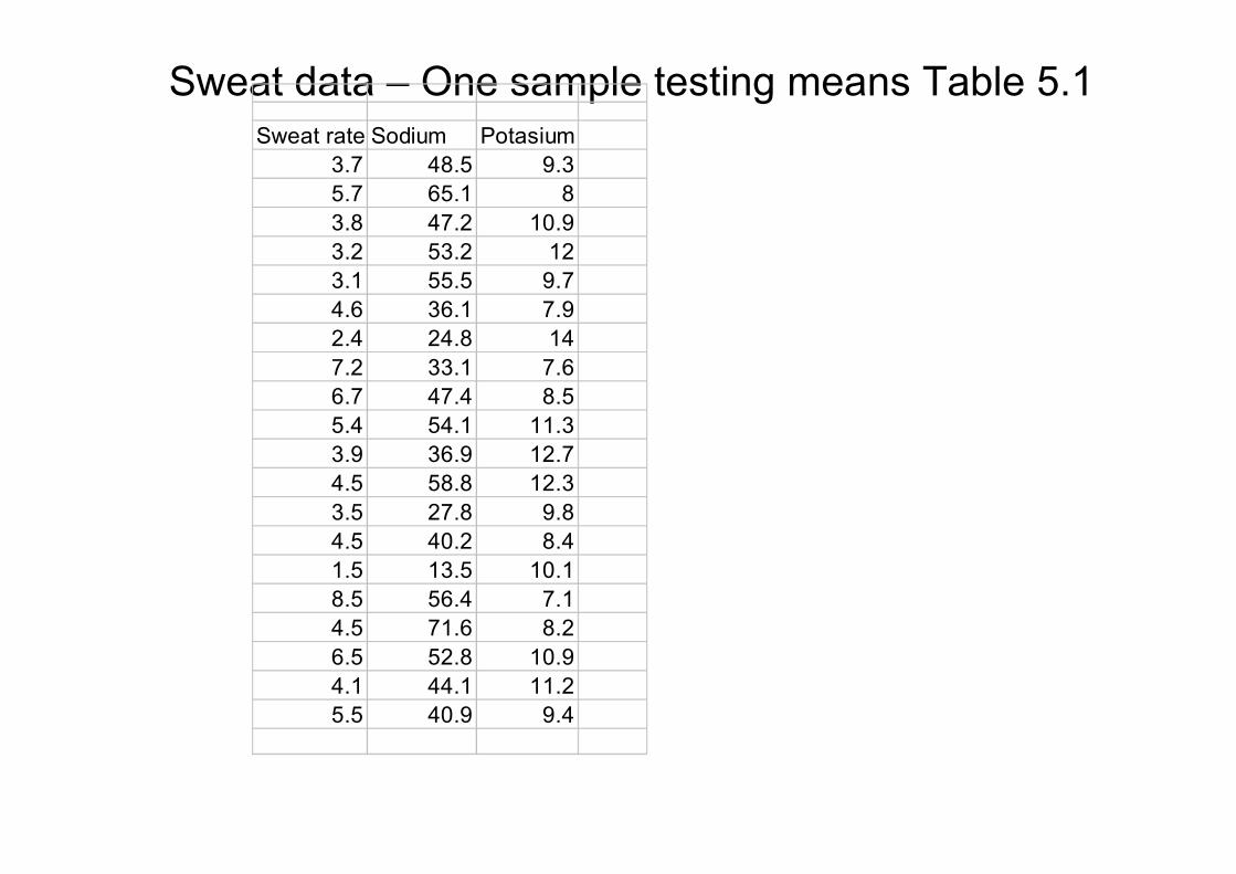
Sweat data – One sample testing means Table 5.1Sweat rate Sodium Potasium
3.7 48.5 9.3
5.7 65.1 8
3.8 47.2 10.9
3.2 53.2 12
3.1 55.5 9.7
4.6 36.1 7.9
2.4 24.8 14
7.2 33.1 7.6
6.7 47.4 8.5
5.4 54.1 11.3
3.9 36.9 12.7
4.5 58.8 12.3
3.5 27.8 9.8
4.5 40.2 8.4
1.5 13.5 10.1
8.5 56.4 7.1
4.5 71.6 8.2
6.5 52.8 10.9
4.1 44.1 11.2
5.5 40.9 9.4
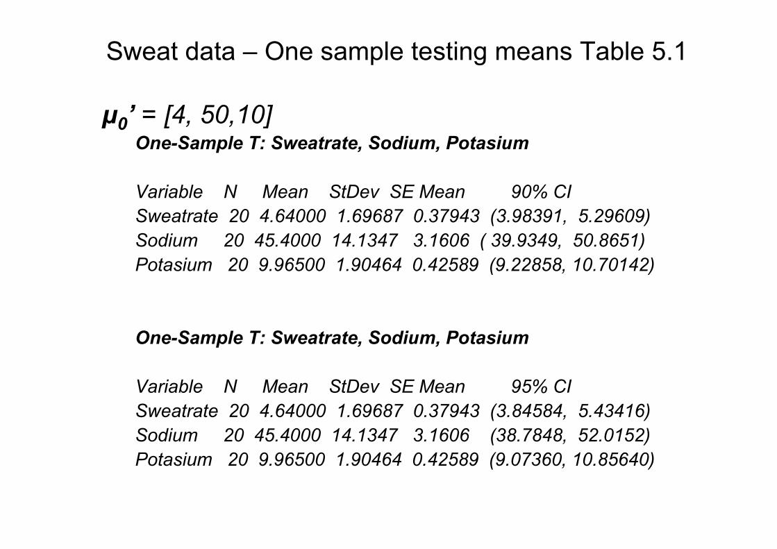
Sweat data – One sample testing means Table 5.1
µ0’ = [4, 50,10]One-Sample T: Sweatrate, Sodium, Potasium
Variable N Mean StDev SE Mean 90% CI
Sweatrate 20 4.64000 1.69687 0.37943 (3.98391, 5.29609)
Sodium 20 45.4000 14.1347 3.1606 ( 39.9349, 50.8651)
Potasium 20 9.96500 1.90464 0.42589 (9.22858, 10.70142)
One-Sample T: Sweatrate, Sodium, Potasium
Variable N Mean StDev SE Mean 95% CI
Sweatrate 20 4.64000 1.69687 0.37943 (3.84584, 5.43416)
Sodium 20 45.4000 14.1347 3.1606 (38.7848, 52.0152)
Potasium 20 9.96500 1.90464 0.42589 (9.07360, 10.85640)

Sweat data – One sample testing means Table 5.1
µ0’ = [4, 50,10]
0.401847 -0.001580.257969Potasium
=20*.487=9.74(Xbar-Miu0)’S(-1)n*(Xbar-Miu0)’
F(3,17,.9)=3.20F(3,17,.9)=2.44=2.905F=(n-p)/[(n-1)*p]*T2
-0.001580.006067-0.02209Sodium
0.257969-0.022090.586155Sweat rate
PotasiumSodiumSweat rateS-matrix(-1)
3.627658-5.64-1.80905Potasium
-5.64199.788410.01Sodium
-1.8090510.012.879368Sweat rate
PotasiumSodiumSweat rateS-matrix
Xbar-Miu0-0.035-4.60.64
Miu010504
Means9.96545.44.64
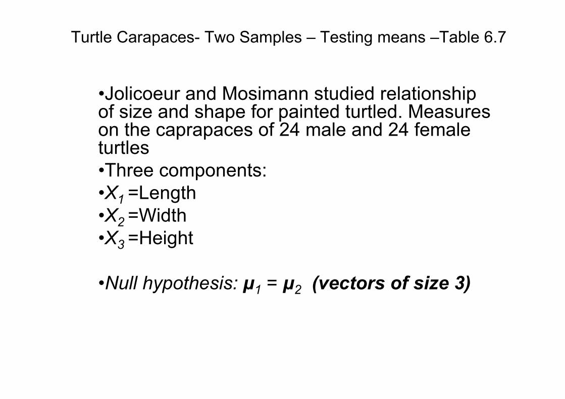
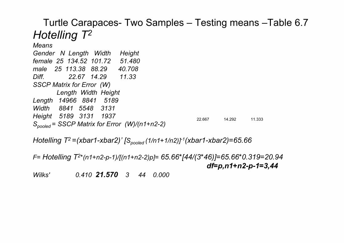
Turtle Carapaces- Two Samples – Testing means –Table 6.7
•Jolicoeur and Mosimann studied relationship of size and shape for painted turtled. Measures on the caprapaces of 24 male and 24 female turtles
•Three components:
•X1 =Length
•X2 =Width
•X3 =Height
•Null hypothesis: µ1 = µ2 (vectors of size 3)
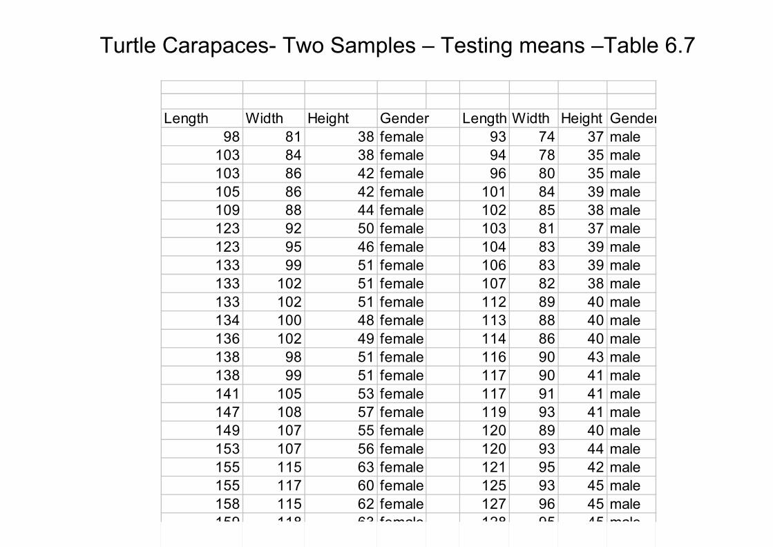
Turtle Carapaces- Two Samples – Testing means –Table 6.7
Length Width Height Gender Length Width Height Gender
98 81 38 female 93 74 37 male
103 84 38 female 94 78 35 male
103 86 42 female 96 80 35 male
105 86 42 female 101 84 39 male
109 88 44 female 102 85 38 male
123 92 50 female 103 81 37 male
123 95 46 female 104 83 39 male
133 99 51 female 106 83 39 male
133 102 51 female 107 82 38 male
133 102 51 female 112 89 40 male
134 100 48 female 113 88 40 male
136 102 49 female 114 86 40 male
138 98 51 female 116 90 43 male
138 99 51 female 117 90 41 male
141 105 53 female 117 91 41 male
147 108 57 female 119 93 41 male
149 107 55 female 120 89 40 male
153 107 56 female 120 93 44 male
155 115 63 female 121 95 42 male
155 117 60 female 125 93 45 male
158 115 62 female 127 96 45 male
159 118 63 female 128 95 45 male
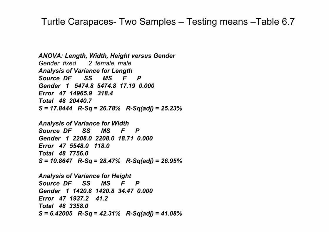
Turtle Carapaces- Two Samples – Testing means –Table 6.7
ANOVA: Length, Width, Height versus Gender
Gender fixed 2 female, male
Analysis of Variance for Length
Source DF SS MS F P
Gender 1 5474.8 5474.8 17.19 0.000
Error 47 14965.9 318.4
Total 48 20440.7
S = 17.8444 R-Sq = 26.78% R-Sq(adj) = 25.23%
Analysis of Variance for Width
Source DF SS MS F P
Gender 1 2208.0 2208.0 18.71 0.000
Error 47 5548.0 118.0
Total 48 7756.0
S = 10.8647 R-Sq = 28.47% R-Sq(adj) = 26.95%
Analysis of Variance for Height
Source DF SS MS F P
Gender 1 1420.8 1420.8 34.47 0.000
Error 47 1937.2 41.2
Total 48 3358.0
S = 6.42005 R-Sq = 42.31% R-Sq(adj) = 41.08%
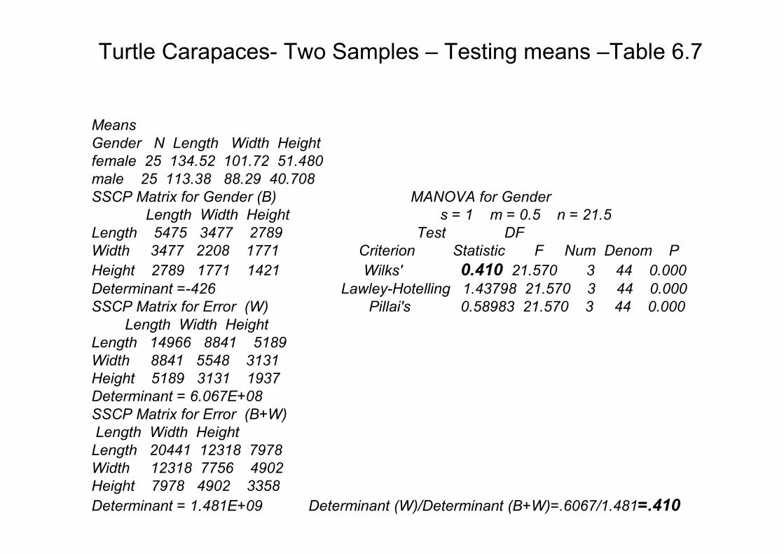
Turtle Carapaces- Two Samples – Testing means –Table 6.7
Means
Gender N Length Width Height
female 25 134.52 101.72 51.480
male 25 113.38 88.29 40.708
SSCP Matrix for Gender (B) MANOVA for Gender
Length Width Height s = 1 m = 0.5 n = 21.5
Length 5475 3477 2789 Test DF
Width 3477 2208 1771 Criterion Statistic F Num Denom P
Height 2789 1771 1421 Wilks' 0.410 21.570 3 44 0.000
Determinant =-426 Lawley-Hotelling 1.43798 21.570 3 44 0.000
SSCP Matrix for Error (W) Pillai's 0.58983 21.570 3 44 0.000
Length Width Height
Length 14966 8841 5189
Width 8841 5548 3131
Height 5189 3131 1937
Determinant = 6.067E+08
SSCP Matrix for Error (B+W)
Length Width Height
Length 20441 12318 7978
Width 12318 7756 4902
Height 7978 4902 3358
Determinant = 1.481E+09 Determinant (W)/Determinant (B+W)=.6067/1.481=.410

Notations for MANOVA-
Exact F-distributions for Wilk’s Lambda
~ )( )( : 2 )
~ )( )( : 2 )
~ )( )( : 1)
~ )( )( : 1)
)1,min(way}-One {),min(
way)-Onein ( E of
way)-Onein 1-( (H) Hypothesis of
MANOVAin Denote
)1(2,2
11
)1(2,211
1,
11
,1
pvpp
pv
vqqv
pvpp
pv
vqqv
FFqd
FFpc
FF qb
FF pa
gpInqps
N-gdfv
gdfq
−+
−+
Λ
Λ−
−
−
Λ
Λ−
−+
−+
Λ
Λ−
Λ
Λ−
==
==
==
==
−==
=
=
Turtle Carapaces- Two Samples – Testing means –Table 6.7
Hotelling T2Means
Gender N Length Width Height
female 25 134.52 101.72 51.480
male 25 113.38 88.29 40.708
Diff. 22.67 14.29 11.33
SSCP Matrix for Error (W)
Length Width Height
Length 14966 8841 5189
Width 8841 5548 3131
Height 5189 3131 1937
Spooled = SSCP Matrix for Error (W)/(n1+n2-2)
Hotelling T2 =(xbar1-xbar2)’ [Spooled (1/n1+1/n2)]-1(xbar1-xbar2)=65.66
F= Hotelling T2*(n1+n2-p-1)/[(n1+n2-2)p]= 65.66*[44/(3*46)]=65.66*0.319=20.94
df=p,n1+n2-p-1=3,44
Wilks' 0.410 21.570 3 44 0.000
11.333 14.292 22.667

Amitriptyline Data –Multivariate Regression Analysis - Table7.6
•Amitriptyline – drug for depression. Several side effects: irregular heartbeat, abnormal BP, etc. Data on 17 patients admited after amitriptyline overdose Two dependent variables and 5 predictor variables:
•Y1 =Total TCAD plasma level (TOT)
•Y2 =Amount of amitriptyline in TCAD plasma level (AMI)
•z1 =Gender 1=female, 0=male
•z2 =Amount of amitriptyline taken at time of overdose(AMT)
•z3 =PR wave measurements (PR)
•z4 =Diastolic blood pressure (DIAP)
•z5 =QRS wave measurements (QRS)
•Analysis: Model to predict Y1 and Y2 from the predictor variables
•Multivariate Linear Regression Models
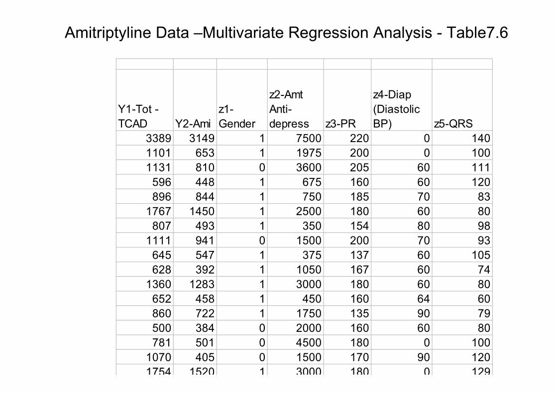
Amitriptyline Data –Multivariate Regression Analysis - Table7.6
Y1-Tot -
TCAD Y2-Ami
z1-
Gender
z2-Amt
Anti-
depress z3-PR
z4-Diap
(Diastolic
BP) z5-QRS
3389 3149 1 7500 220 0 140
1101 653 1 1975 200 0 100
1131 810 0 3600 205 60 111
596 448 1 675 160 60 120
896 844 1 750 185 70 83
1767 1450 1 2500 180 60 80
807 493 1 350 154 80 98
1111 941 0 1500 200 70 93
645 547 1 375 137 60 105
628 392 1 1050 167 60 74
1360 1283 1 3000 180 60 80
652 458 1 450 160 64 60
860 722 1 1750 135 90 79
500 384 0 2000 160 60 80
781 501 0 4500 180 0 100
1070 405 0 1500 170 90 120
1754 1520 1 3000 180 0 129

Amitriptyline Data –Multivariate Regression Analysis - Table7.6
•Multivariate Linear Regression ModelsRegression Analysis: Y1 versus Z1, Z2, Z3, Z4, Z5
The regression equation is
Y1 = - 2879 + 676 Z1 + 0.285 Z2 + 10.3 Z3 + 7.25 Z4 + 7.60 Z5
Predictor Coef SE Coef T P
Constant -2879.5 893.3 -3.22 0.008
Z1 675.7 162.1 4.17 0.002
Z2 0.28485 0.06091 4.68 0.001
Z3 10.272 4.255 2.41 0.034
Z4 7.251 3.225 2.25 0.046
Z5 7.598 3.849 1.97 0.074
S = 281.232 R-Sq = 88.7% R-Sq(adj) = 83.6%
Analysis of Variance
Source DF SS MS F P
Regression 5 6835932 1367186 17.29 0.000
Residual Error 11 870008 79092
Total 16 7705940

Amitriptyline Data –Multivariate Regression Analysis - Table7.6
•Multivariate Linear Regression ModelsRegression Analysis: Y2 versus Z1, Z2, Z3, Z4, Z5
The regression equation is
Y2 = - 2729 + 763 Z1 + 0.306 Z2 + 8.90 Z3 + 7.21 Z4 + 4.99 Z5
Predictor Coef SE Coef T P
Constant -2728.7 928.8 -2.94 0.014
Z1 763.0 168.5 4.53 0.001
Z2 0.30637 0.06334 4.84 0.001
Z3 8.896 4.424 2.01 0.070
Z4 7.206 3.354 2.15 0.055
Z5 4.987 4.002 1.25 0.239
Analysis of Variance
Source DF SS MS F P
Regression 5 6669669 1333934 15.60 0.000
Residual Error 11 940709 85519
Total 16 7610378
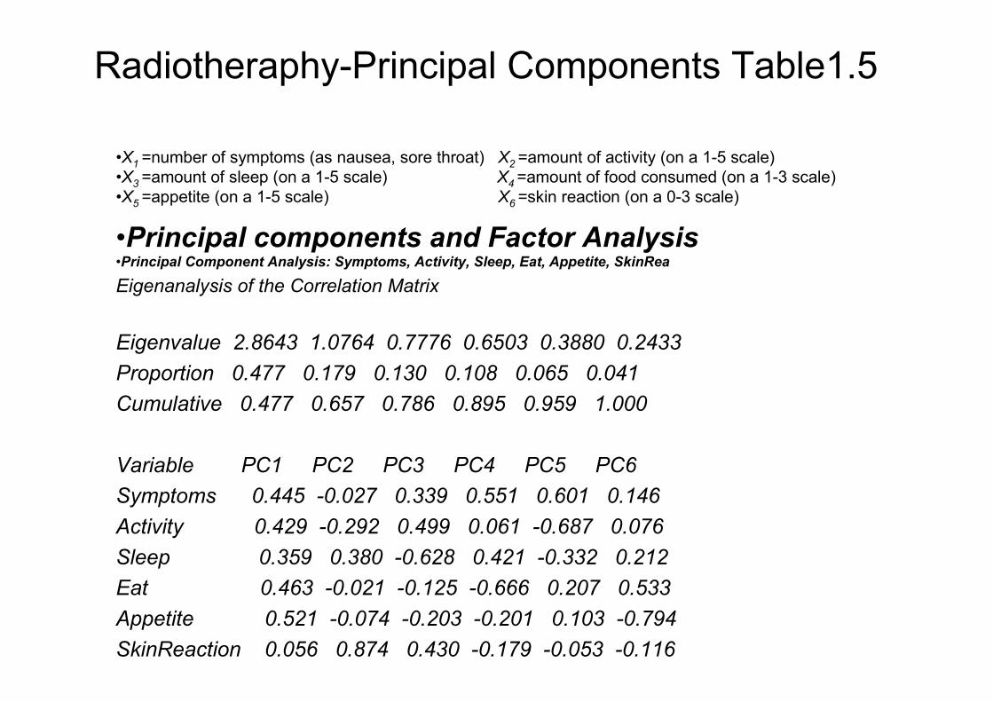
Radiotheraphy-Principal Components Table1.5
•Data of the 98 average ratings over the course of the treatment for 98 patients undergoing radiotherapy. Six components:
•X1 =number of symptoms (as nausea, sore throat)
•X2 =amount of activity (on a 1-5 scale)
•X3 =amount of sleep (on a 1-5 scale)
•X4 =amount of food consumed (on a 1-3 scale)
•X5 =appetite (on a 1-5 scale)
•X6 =skin reaction (on a 0-3 scale)
•Analysis: Finding a single (or several) measures – linear combinations of the 6 components, to represent patients’response to therapy.
•Principal components
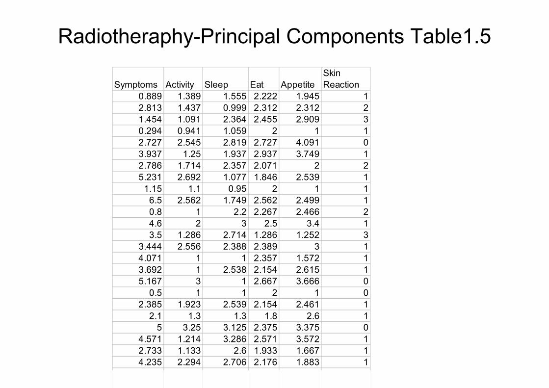
Radiotheraphy-Principal Components Table1.5
Symptoms Activity Sleep Eat Appetite
Skin
Reaction
0.889 1.389 1.555 2.222 1.945 1
2.813 1.437 0.999 2.312 2.312 2
1.454 1.091 2.364 2.455 2.909 3
0.294 0.941 1.059 2 1 1
2.727 2.545 2.819 2.727 4.091 0
3.937 1.25 1.937 2.937 3.749 1
2.786 1.714 2.357 2.071 2 2
5.231 2.692 1.077 1.846 2.539 1
1.15 1.1 0.95 2 1 1
6.5 2.562 1.749 2.562 2.499 1
0.8 1 2.2 2.267 2.466 2
4.6 2 3 2.5 3.4 1
3.5 1.286 2.714 1.286 1.252 3
3.444 2.556 2.388 2.389 3 1
4.071 1 1 2.357 1.572 1
3.692 1 2.538 2.154 2.615 1
5.167 3 1 2.667 3.666 0
0.5 1 1 2 1 0
2.385 1.923 2.539 2.154 2.461 1
2.1 1.3 1.3 1.8 2.6 1
5 3.25 3.125 2.375 3.375 0
4.571 1.214 3.286 2.571 3.572 1
2.733 1.133 2.6 1.933 1.667 1
4.235 2.294 2.706 2.176 1.883 1
0 1 1.941 2 2 0
Radiotheraphy-Principal Components Table1.5
•X1 =number of symptoms (as nausea, sore throat) X2 =amount of activity (on a 1-5 scale)
•X3 =amount of sleep (on a 1-5 scale) X4 =amount of food consumed (on a 1-3 scale)
•X5 =appetite (on a 1-5 scale) X6 =skin reaction (on a 0-3 scale)
•Principal components and Factor Analysis•Principal Component Analysis: Symptoms, Activity, Sleep, Eat, Appetite, SkinRea
Eigenanalysis of the Correlation Matrix
Eigenvalue 2.8643 1.0764 0.7776 0.6503 0.3880 0.2433
Proportion 0.477 0.179 0.130 0.108 0.065 0.041
Cumulative 0.477 0.657 0.786 0.895 0.959 1.000
Variable PC1 PC2 PC3 PC4 PC5 PC6
Symptoms 0.445 -0.027 0.339 0.551 0.601 0.146
Activity 0.429 -0.292 0.499 0.061 -0.687 0.076
Sleep 0.359 0.380 -0.628 0.421 -0.332 0.212
Eat 0.463 -0.021 -0.125 -0.666 0.207 0.533
Appetite 0.521 -0.074 -0.203 -0.201 0.103 -0.794
SkinReaction 0.056 0.874 0.430 -0.179 -0.053 -0.116
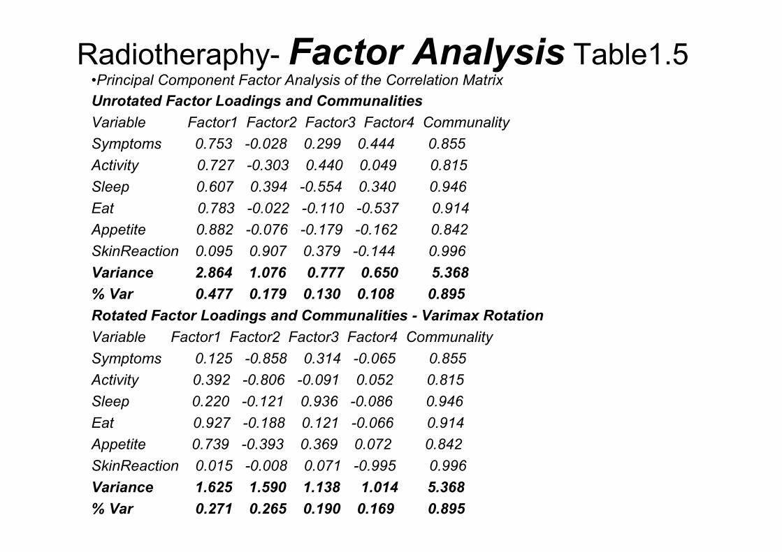
Radiotheraphy- Factor Analysis Table1.5•Principal Component Factor Analysis of the Correlation Matrix
Unrotated Factor Loadings and Communalities
Variable Factor1 Factor2 Factor3 Factor4 Communality
Symptoms 0.753 -0.028 0.299 0.444 0.855
Activity 0.727 -0.303 0.440 0.049 0.815
Sleep 0.607 0.394 -0.554 0.340 0.946
Eat 0.783 -0.022 -0.110 -0.537 0.914
Appetite 0.882 -0.076 -0.179 -0.162 0.842
SkinReaction 0.095 0.907 0.379 -0.144 0.996
Variance 2.864 1.076 0.777 0.650 5.368
% Var 0.477 0.179 0.130 0.108 0.895
Rotated Factor Loadings and Communalities - Varimax Rotation
Variable Factor1 Factor2 Factor3 Factor4 Communality
Symptoms 0.125 -0.858 0.314 -0.065 0.855
Activity 0.392 -0.806 -0.091 0.052 0.815
Sleep 0.220 -0.121 0.936 -0.086 0.946
Eat 0.927 -0.188 0.121 -0.066 0.914
Appetite 0.739 -0.393 0.369 0.072 0.842
SkinReaction 0.015 -0.008 0.071 -0.995 0.996
Variance 1.625 1.590 1.138 1.014 5.368
% Var 0.271 0.265 0.190 0.169 0.895
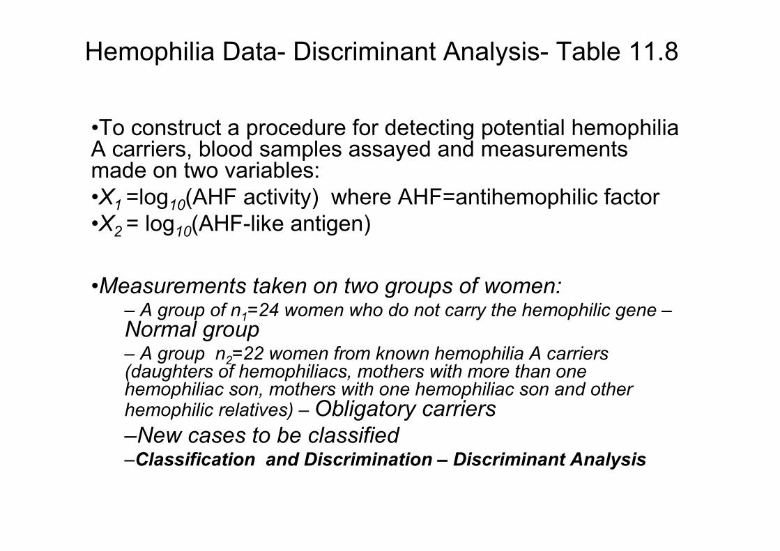
Hemophilia Data- Discriminant Analysis- Table 11.8
•To construct a procedure for detecting potential hemophilia A carriers, blood samples assayed and measurements made on two variables:
•X1 =log10(AHF activity) where AHF=antihemophilic factor
•X2 = log10(AHF-like antigen)
•Measurements taken on two groups of women:– A group of n1=24 women who do not carry the hemophilic gene –Normal group– A group n2=22 women from known hemophilia A carriers (daughters of hemophiliacs, mothers with more than one hemophiliac son, mothers with one hemophiliac son and other hemophilic relatives) –Obligatory carriers
–New cases to be classified–Classification and Discrimination – Discriminant Analysis

Hemophilia Data- Discriminant Analysis- Table 11.8
Noncarriers Obligatory Carriers New cases Requiring Classification
Group
log(AHF
activity)
log(AHF
antigen) Group
log(AHF
activity)
log(AHF
antigen) Group
log(AHF
activity)
log(AHF
antigen)
1 -0.0056 -0.1657 2 -0.3478 0.1151 3 -0.112 -0.279
1 -0.1698 -0.1585 2 -0.3618 -0.2008 3 -0.059 -0.068
1 -0.3469 -0.1879 2 -0.4986 -0.086 3 0.064 0.012
1 -0.0894 0.0064 2 -0.5015 -0.2984 3 -0.043 -0.052
1 -0.1679 0.0713 2 -0.1326 0.0097 3 -0.05 -0.098
1 -0.0836 0.0106 2 -0.6911 -0.339 3 -0.094 -0.113
1 -0.1979 -0.0005 2 -0.3608 0.1237 3 -0.123 -0.143
1 -0.0762 0.0392 2 -0.4535 -0.1682 3 -0.011 -0.037
1 -0.1913 -0.2123 2 -0.3479 -0.1721 3 -0.21 -0.09
1 -0.1092 -0.119 2 -0.3539 0.0722 3 -0.126 -0.019
1 -0.5268 -0.4773 2 -0.4719 -0.1079
1 -0.0842 0.0248 2 -0.361 -0.0399
1 -0.0225 -0.058 2 -0.3226 0.167
1 0.0084 0.0782 2 -0.4319 -0.0687
1 -0.1827 -0.1138 2 -0.2734 -0.002
1 0.1237 0.214 2 -0.5573 0.0548
1 -0.4702 -0.3099 2 -0.3755 -0.1865
1 -0.1519 -0.0686 2 -0.495 -0.0153
1 0.0006 -0.1153 2 -0.5107 -0.2483
1 -0.2015 -0.0498 2 -0.1652 0.2132
1 -0.1932 -0.2293 2 -0.2447 -0.0407
1 0.1507 0.0933 2 -0.4232 -0.0998
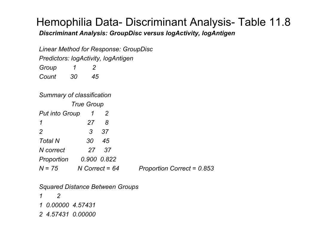
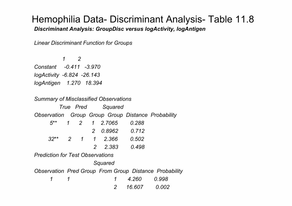
Hemophilia Data- Discriminant Analysis- Table 11.8Discriminant Analysis: GroupDisc versus logActivity, logAntigen
Linear Method for Response: GroupDisc
Predictors: logActivity, logAntigen
Group 1 2
Count 30 45
Summary of classification
True Group
Put into Group 1 2
1 27 8
2 3 37
Total N 30 45
N correct 27 37
Proportion 0.900 0.822
N = 75 N Correct = 64 Proportion Correct = 0.853
Squared Distance Between Groups
1 2
1 0.00000 4.57431
2 4.57431 0.00000
Hemophilia Data- Discriminant Analysis- Table 11.8Discriminant Analysis: GroupDisc versus logActivity, logAntigen
Linear Discriminant Function for Groups
1 2
Constant -0.411 -3.970
logActivity -6.824 -26.143
logAntigen 1.270 18.394
Summary of Misclassified Observations
True Pred Squared
Observation Group Group Group Distance Probability
5** 1 2 1 2.7065 0.288
2 0.8962 0.712
32** 2 1 1 2.366 0.502
2 2.383 0.498
Prediction for Test Observations
Squared
Observation Pred Group From Group Distance Probability
1 1 1 4.260 0.998
2 16.607 0.002

Hemophilia Data- Discriminant Analysis- Table 11.8Discriminant Analysis: -Minitab
Distance and discriminant functions
Squared distance: The squared distance (also called the Mahalanobisdistance) of observation x to the center (mean) of group i is given by the general form:
di2 (x) = (x - mi)' Sp
-1 (x - mi) where: x = p-column vector with the values of this observation
mi = column vector of length p containing the means of the predictors calculated from the data in group i;
Sp = pooled covariance matrix, used in linear discriminant analysis;
The linear discriminant function =mi' Sp-1x - 0.5mi'Sp
-1mi + ln p where:
x = column vector of length p containing the values of the predictors for this observation (note, this column vector is stored as one row)
mi = column vector of length p containing the means of the predictors calculated from the data in group i
Sp = pooled covariance matrix
ln p = natural log of the prior probability
For a given x, the group with the smallest squared distance has the largest linear discriminant function.
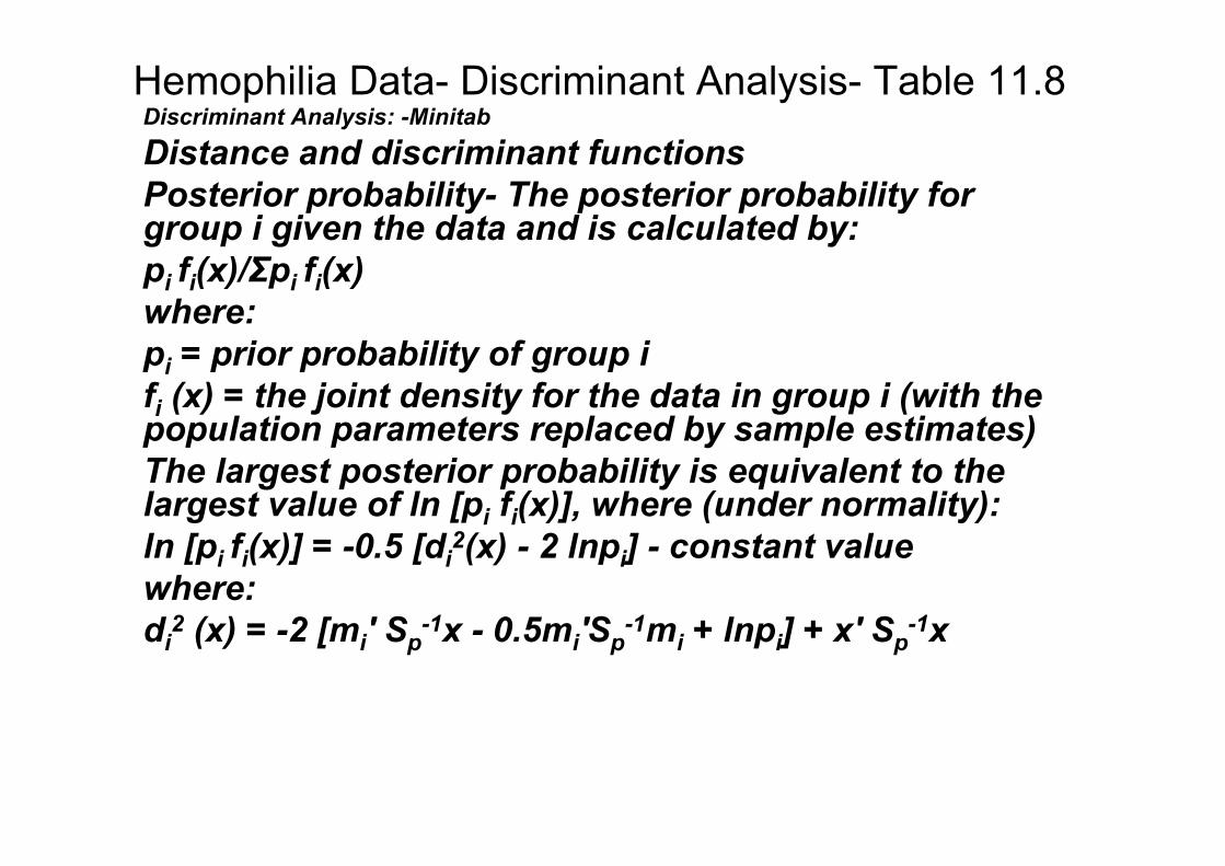
Hemophilia Data- Discriminant Analysis- Table 11.8Discriminant Analysis: -Minitab
Distance and discriminant functions
Posterior probability- The posterior probability for group i given the data and is calculated by:
pi fi(x)/Σpi fi(x)
where:
pi = prior probability of group i
fi (x) = the joint density for the data in group i (with the population parameters replaced by sample estimates)
The largest posterior probability is equivalent to the largest value of ln [pi fi(x)], where (under normality):
ln [pi fi(x)] = -0.5 [di2(x) - 2 lnpi] - constant value
where:
di2 (x) = -2 [mi' Sp
-1x - 0.5mi'Sp-1mi + lnpi] + x' Sp
-1x

Bone and Skull - White leghorn fowls –
Canonical Correlation- Ex10.4
•To assess correlation between two sets of variables
•Head Measurements (X(1) )–X(1)1 =Skull length
–X(1)2 =Skull breadth
•Leg Measurements (X(1) )–X(2)1 =Femur length
–X(2)2 =Tibia length
–Create new variables which represent the most of the correlations between the two sets of variables –
–Cannonical Correlation
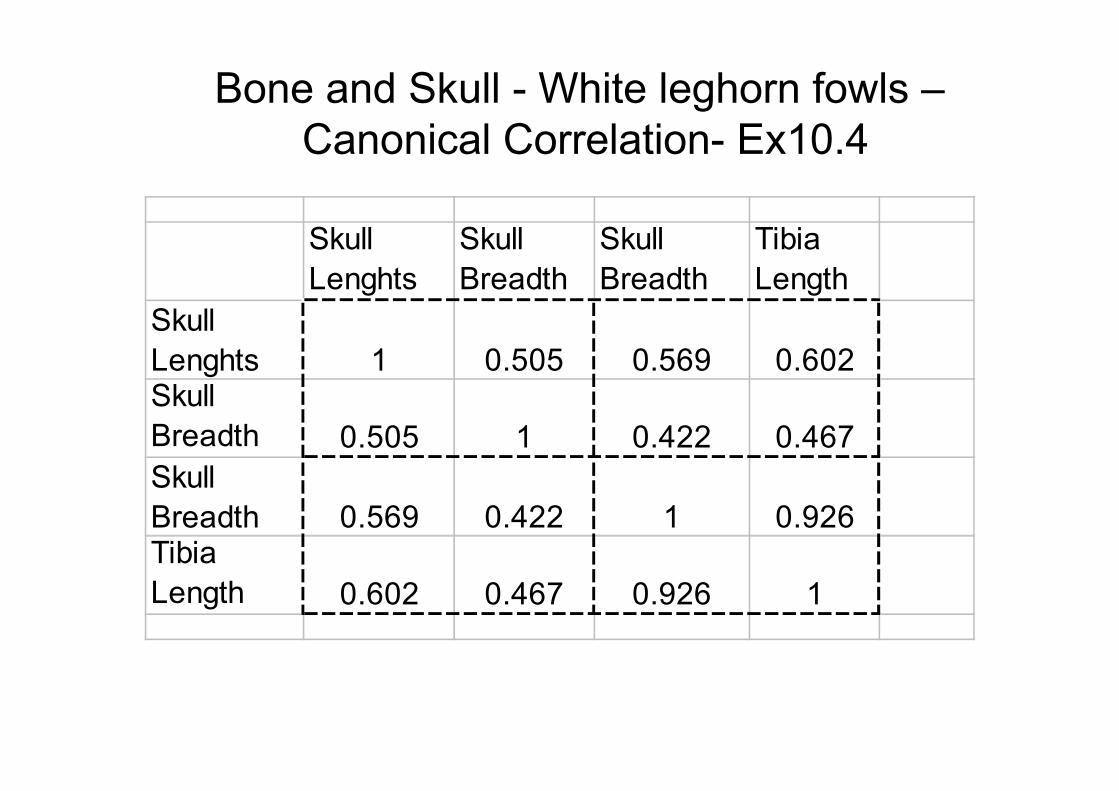
Bone and Skull - White leghorn fowls –
Canonical Correlation- Ex10.4
Skull
Lenghts
Skull
Breadth
Skull
Breadth
Tibia
Length
Skull
Lenghts 1 0.505 0.569 0.602Skull
Breadth 0.505 1 0.422 0.467
Skull
Breadth 0.569 0.422 1 0.926Tibia
Length 0.602 0.467 0.926 1
Universities – Cluster Analysis-Table 12-9
•Data on certain universities for certain variables used to compare or rank major universities. The variables:
•X1 =Average SAT for new freshmen
•X2 = Percent new freshmen in top 10% of high school class
•X3 =Percent of applicants accepted
•X4 =Student faculty ratio
•X5 =Estimated annual expenses
•X6 =Graduation rate (%)
•Analysis: Clustering observations (universities) based on linear combinations of variables (or specific variables). Definition of distances
•Cluster Analysis, Distance Methods and Ordination

Universities – Cluster Analysis-Table 12-9# SAT Top10 Accept SFRatio Expenses
1 Harvard 14.00 91 14 11 39.525
2 Princeton 13.75 91 14 8 30.220
3 Yale 13.75 95 19 11 43.514
4 Stanford 13.60 90 20 12 36.450
5 MIT 13.80 94 30 10 34.870
6 Duke 13.15 90 30 12 31.585
7 CalTech 14.15 100 25 6 63.575
8 Dartmouth 13.40 89 23 10 32.162
9 Brown 13.10 89 22 13 22.704
10 JohnsHopkins 13.05 75 44 7 58.691
11 Uchicago 12.90 75 50 13 38.380
12 UPenn 12.85 80 36 11 27.553
13 Cornell 12.80 83 33 13 21.860
14 Northwestern 12.60 85 39 11 28.052
15 Columbia 13.10 76 24 12 31.510
16 NotreDame 12.55 81 42 13 15.122
17 UVir 12.25 77 44 14 13.349
18 Georgetown 12.55 74 24 12 20.126
19 CarnegieMellon 12.60 62 59 9 25.026
20 Umichigan 11.80 65 68 16 15.470
21 UCBerkeley 12.40 95 40 17 15.140
22 Uwisconsin 10.85 40 69 15 11.857
23 PennState 10.81 38 54 18 10.180
24 Purdue 10.05 28 90 19 9.066
25 TexasA&M 10.75 49 67 25 8.704
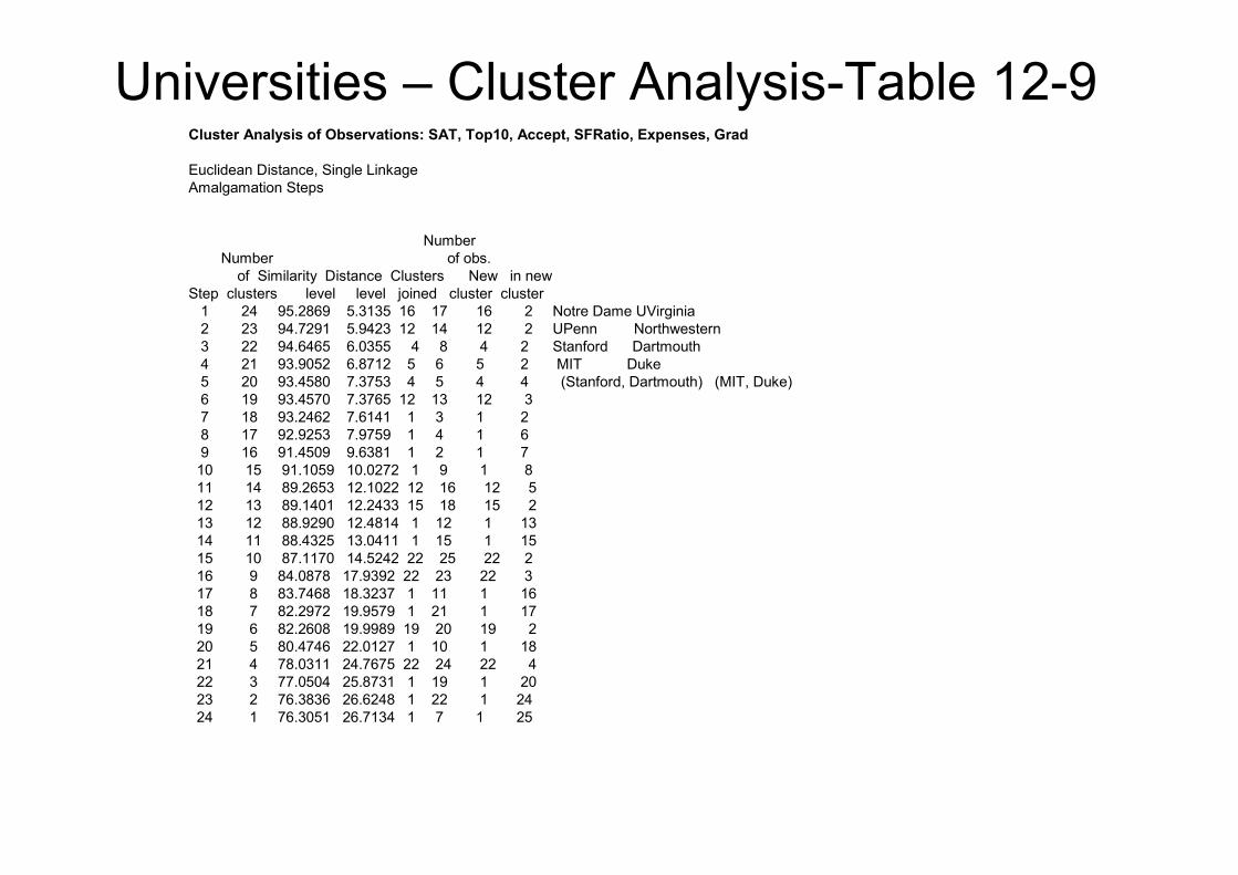
Universities – Cluster Analysis-Table 12-9Cluster Analysis of Observations: SAT, Top10, Accept, SFRatio, Expenses, Grad
Euclidean Distance, Single Linkage
Amalgamation Steps
Number
Number of obs.
of Similarity Distance Clusters New in new
Step clusters level level joined cluster cluster
1 24 95.2869 5.3135 16 17 16 2 Notre Dame UVirginia
2 23 94.7291 5.9423 12 14 12 2 UPenn Northwestern
3 22 94.6465 6.0355 4 8 4 2 Stanford Dartmouth
4 21 93.9052 6.8712 5 6 5 2 MIT Duke
5 20 93.4580 7.3753 4 5 4 4 (Stanford, Dartmouth) (MIT, Duke)
6 19 93.4570 7.3765 12 13 12 3
7 18 93.2462 7.6141 1 3 1 2
8 17 92.9253 7.9759 1 4 1 6
9 16 91.4509 9.6381 1 2 1 7
10 15 91.1059 10.0272 1 9 1 8
11 14 89.2653 12.1022 12 16 12 5
12 13 89.1401 12.2433 15 18 15 2
13 12 88.9290 12.4814 1 12 1 13
14 11 88.4325 13.0411 1 15 1 15
15 10 87.1170 14.5242 22 25 22 2
16 9 84.0878 17.9392 22 23 22 3
17 8 83.7468 18.3237 1 11 1 16
18 7 82.2972 19.9579 1 21 1 17
19 6 82.2608 19.9989 19 20 19 2
20 5 80.4746 22.0127 1 10 1 18
21 4 78.0311 24.7675 22 24 22 4
22 3 77.0504 25.8731 1 19 1 20
23 2 76.3836 26.6248 1 22 1 24
24 1 76.3051 26.7134 1 7 1 25
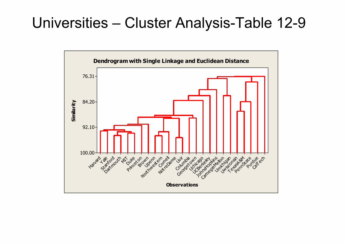
Universities – Cluster Analysis-Table 12-9
Observations
Similarity
CalTech
Purdue
PennState
TexasA&M
Uwisconsin
Umichigan
CarnegieMellon
JohnsHopkins
UCBerkeley
Uchicago
Georgetown
Columbia
Uvir
NotreDame
Cornell
Northwestern
Upenn
Brown
Princeton
Duke
MIT
Dartmouth
Stanford
Yale
Harvard
76.31
84.20
92.10
100.00
Dendrogram with Single Linkage and Euclidean Distance
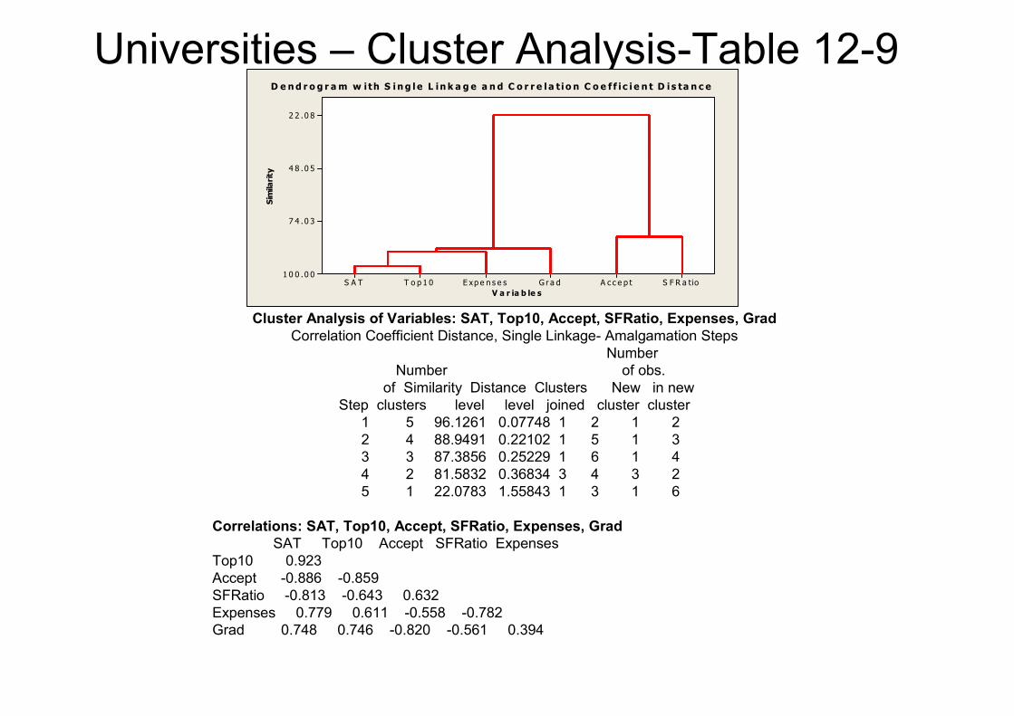
Universities – Cluster Analysis-Table 12-9
Cluster Analysis of Variables: SAT, Top10, Accept, SFRatio, Expenses, Grad
Correlation Coefficient Distance, Single Linkage- Amalgamation Steps
Number
Number of obs.
of Similarity Distance Clusters New in new
Step clusters level level joined cluster cluster
1 5 96.1261 0.07748 1 2 1 2
2 4 88.9491 0.22102 1 5 1 3
3 3 87.3856 0.25229 1 6 1 4
4 2 81.5832 0.36834 3 4 3 2
5 1 22.0783 1.55843 1 3 1 6
Correlations: SAT, Top10, Accept, SFRatio, Expenses, Grad
SAT Top10 Accept SFRatio Expenses
Top10 0.923
Accept -0.886 -0.859
SFRatio -0.813 -0.643 0.632
Expenses 0.779 0.611 -0.558 -0.782
Grad 0.748 0.746 -0.820 -0.561 0.394
V a r ia b le s
Similarity
S F R a tioA c c e p tG r a dE xp e n s e sT o p 1 0S A T
2 2 .0 8
4 8 .0 5
7 4 .0 3
1 0 0 .0 0
D e nd r o g r am w i th S i n g l e L in k a g e a n d C o r r e l a t i o n C o e f f i c i e n t D i s ta n c e
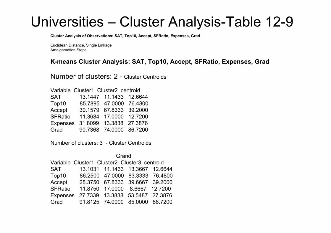
Universities – Cluster Analysis-Table 12-9Cluster Analysis of Observations: SAT, Top10, Accept, SFRatio, Expenses, Grad
Euclidean Distance, Single Linkage
Amalgamation Steps
K-means Cluster Analysis: SAT, Top10, Accept, SFRatio, Expenses, Grad
Number of clusters: 2 - Cluster Centroids
Variable Cluster1 Cluster2 centroid
SAT 13.1447 11.1433 12.6644
Top10 85.7895 47.0000 76.4800
Accept 30.1579 67.8333 39.2000
SFRatio 11.3684 17.0000 12.7200
Expenses 31.8099 13.3838 27.3876
Grad 90.7368 74.0000 86.7200
Number of clusters: 3 - Cluster Centroids
Grand
Variable Cluster1 Cluster2 Cluster3 centroid
SAT 13.1031 11.1433 13.3667 12.6644
Top10 86.2500 47.0000 83.3333 76.4800
Accept 28.3750 67.8333 39.6667 39.2000
SFRatio 11.8750 17.0000 8.6667 12.7200
Expenses 27.7339 13.3838 53.5487 27.3876
Grad 91.8125 74.0000 85.0000 86.7200