Multivariable control of an industrial boiler-turbine unit with ...scientiairanica.sharif.edu/article_3406_f2afd3e6735ec841c70e77... · controllers based on LQG/LQR theory cannot

Scientia Iranica B (2013) 20(5), 1485{1498

Sharif University of TechnologyScientia Iranica

Transactions B: Mechanical Engineeringwww.scientiairanica.com

Multivariable control of an industrial boiler-turbineunit with nonlinear model: A comparison between gainscheduling and feedback linearization approaches

H. Moradia;�, A. Alastya, M. Sa�ar-Avvalb and F. Bakhtiari-Nejadb

a. Centre of Excellence in Design, Robotics & Automation, School of Mechanical Engineering, Sharif University of Technology,Tehran, P.O. Box 11155-9567, Iran.

b. Department of Mechanical Engineering, Amirkabir University of Technology, Tehran, Iran.

Received 20 February 2012; received in revised form 1 January 2013; accepted 25 May 2013

KEYWORDSBoiler-turbine;Nonlinear model;Multivariable control;Gain scheduling;Feedbacklinearization.

Abstract. Due to demands for the economical operations of power plants and envi-ronmental awareness, performance control of a boiler-turbine unit is of great importance.In this paper, a nonlinear Multi Input-Multi Output model (MIMO) of a utility boiler-turbine unit is considered. Drum pressure, generator electric output and drum water level(as the output variables) are controlled by manipulation of valves position for fuel, feed-water and steam ows. After state space representation of the problem, two controllers,based on gain scheduling and feedback linearization, are designed. Tracking performanceof the system is investigated and discussed for three cases of `near', `far' and `so far' set-points. According to the results obtained, using feedback linearization approach leadsto more quick time responses with a bit more overshoots (in comparison with the gainscheduling method). In addition, in feedback linearization strategy, input control signals(valves position) are actuated in less time with less oscillations. It is observed that in thepresence of an arbitrary random uncertainty in model parameters, the controller designedbased on feedback linearization is more robust. Finally, according to the phase portraits ofthe problem, as the desired speed of tracking process is increased, dynamic system tendsto demonstrate a chaotic behaviour.© 2013 Sharif University of Technology. All rights reserved.

1. Introduction

Industrial boiler-turbine units are extensively usedfor steam generation as a source of power or forachieving heating capabilities in thermal plants. Dueto dynamic interaction between various components,such as furnace, evaporator, super-heaters, economizer,attemperator and drum, these units are inherentlynonlinear systems. For the electricity generation,two con�gurations can be realized [1]. In the �rst

*. Corresponding author. Tel.: (+98) 21 66165694,Fax: (+98) 21 66000021E-mail address: [email protected] (H. Moradi)

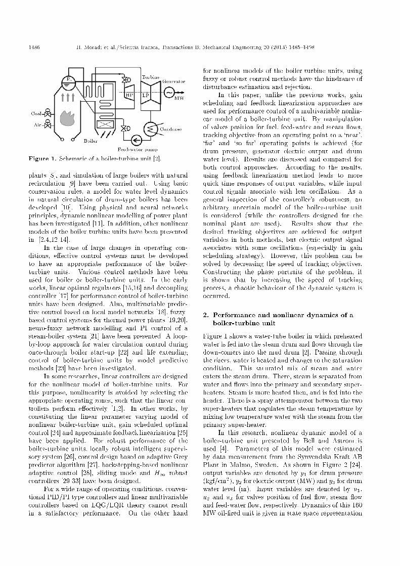
con�guration, as called boiler-turbine unit, the steamis produced by a single boiler and is fed to a singleturbine, as shown in Figure 1 [2]. In the second one,several boilers generate total steam conducted to acollector and then distributed to several turbines. Sincethe boiler-turbine units show quick responses for theelectricity demand from a power network, they arepreferred to collector type systems.

Several dynamic models of the boiler system havebeen developed. In early works, dynamic modellingof a boiler-turbine unit based on data logs, parameterestimation [3-5], system identi�cation [6] and simpli-�cation of nonlinear models [7] has been done. Also,several simulation packages such as SYNSIM for steam

1486 H. Moradi et al./Scientia Iranica, Transactions B: Mechanical Engineering 20 (2013) 1485{1498

Figure 1. Schematic of a boiler-turbine unit [2].

plants [8], and simulation of large boilers with naturalrecirculation [9] have been carried out. Using basicconservation rules, a model for water level dynamicsin natural circulation of drum-type boilers has beendeveloped [10]. Using physical and neural networksprinciples, dynamic nonlinear modelling of power planthas been investigated [11]. In addition, other nonlinearmodels of the boiler-turbine units have been presentedin [2,4,12-14].

In the case of large changes in operating con-ditions, e�ective control systems must be developedto have an appropriate performance of the boiler-turbine units. Various control methods have beenused for boiler or boiler-turbine units. In the earlyworks, linear optimal regulators [15,16] and decouplingcontroller [17] for performance control of boiler-turbineunits have been designed. Also, multivariable predic-tive control based on local model networks [18], fuzzy-based control systems for thermal power plants [19,20],neuro-fuzzy network modelling and PI control of asteam-boiler system [21] have been presented. A loop-by-loop approach for water circulation control duringonce-through boiler start-up [22] and life extendingcontrol of boiler-turbine units by model predictivemethods [23] have been investigated.

In some researches, linear controllers are designedfor the nonlinear model of boiler-turbine units. Forthis purpose, nonlinearity is avoided by selecting theappropriate operating zones, such that the linear con-trollers perform e�ectively [1,2]. In other works, byconstituting the linear parameter varying model ofnonlinear boiler-turbine unit, gain scheduled optimalcontrol [24] and approximate feedback linearization [25]have been applied. For robust performance of theboiler-turbine units, locally robust intelligent supervi-sory system [26], control design based on adaptive Greypredictor algorithm [27], backstepping-based nonlinearadaptive control [28], sliding mode and H1 robustcontrollers [29-33] have been designed.

For a wide range of operating conditions, conven-tional PID/PI type controllers and linear multivariablecontrollers based on LQG/LQR theory cannot resultin a satisfactory performance. On the other hand

for nonlinear models of the boiler-turbine units, usingfuzzy or robust control methods have the hindrance ofdisturbance estimation and rejection.

In this paper, unlike the previous works, gainscheduling and feedback linearization approaches areused for performance control of a multivariable nonlin-ear model of a boiler-turbine unit. By manipulationof valves position for fuel, feed-water and steam ows,tracking objective from an operating point to a `near',`far' and `so far' operating points is achieved (fordrum pressure, generator electric output and drumwater level). Results are discussed and compared forboth control approaches. According to the results,using feedback linearization method leads to morequick time responses of output variables, while inputcontrol signals associate with less oscillation. As ageneral inspection of the controller's robustness, anarbitrary uncertain model of the boiler-turbine unitis considered (while the controllers designed for thenominal plant are used). Results show that thedesired tracking objectives are achieved for outputvariables in both methods, but electric output signalassociates with some oscillations (especially in gainscheduling strategy). However, this problem can besolved by decreasing the speed of tracking objectives.Constructing the phase portraits of the problem, itis shown that by increasing the speed of trackingprocess, a chaotic behaviour of the dynamic system isoccurred.

2. Performance and nonlinear dynamics of aboiler-turbine unit

Figure 1 shows a water-tube boiler in which preheatedwater is fed into the steam drum and ows through thedown-comers into the mud drum [2]. Passing throughthe risers, water is heated and changes to the saturationcondition. This saturated mix of steam and waterenters the steam drum. There, steam is separated fromwater and ows into the primary and secondary super-heaters. Steam is more heated then, and is fed into theheader. There is a spray attemperator between the twosuper-heaters that regulates the steam temperature bymixing low temperature water with the steam from theprimary super-heater.

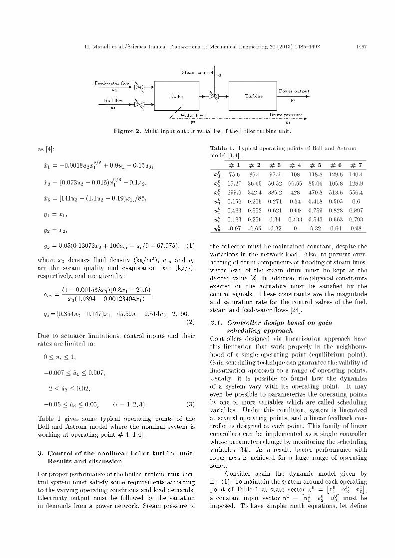
In this research, nonlinear dynamic model of aboiler-turbine unit presented by Bell and Astrom isused [4]. Parameters of this model were estimatedby data measurement from the Synvendska Kraft ABPlant in Malmo, Sweden. As shown in Figure 2 [24],output variables are denoted by y1 for drum pressure(kgf/cm2), y2 for electric output (MW) and y3 for drumwater level (m). Input variables are denoted by u1,u2 and u3 for valves position of fuel ow, steam owand feed-water ow, respectively. Dynamics of this 160MW oil-�red unit is given in state space representation

H. Moradi et al./Scientia Iranica, Transactions B: Mechanical Engineering 20 (2013) 1485{1498 1487

Figure 2. Multi input-output variables of the boiler-turbine unit.

as [4]:

_x1 = �0:0018u2x9=81 + 0:9u1 � 0:15u3;

_x2 = (0:073u2 � 0:016)x9=81 � 0:1x2;

_x3 = [141u3 � (1:1u2 � 0:19)x1]=85;

y1 = x1;

y2 = x2;

y3 = 0:05(0:13073x3 + 100acs + qe=9� 67:975); (1)

where x3 denotes uid density (kg/m3), acs and qeare the steam quality and evaporation rate (kg/s),respectively, and are given by:

acs =(1� 0:001538x3)(0:8x1 � 25:6)x3(1:0394� 0:00123404x1)

;

qe=(0:854u2�0:147)x1+45:59u1�2:514u3�2:096:(2)

Due to actuator limitations, control inputs and theirrates are limited to:

0 � ui � 1;

�0:007 � _u1 � 0:007;

�2 � _u2 � 0:02;

�0:05 � _u3 � 0:05; (i = 1; 2; 3): (3)

Table 1 gives some typical operating points of theBell and Astrom model where the nominal system isworking at operating point # 4 [1,4].

3. Control of the nonlinear boiler-turbine unit:Results and discussion

For proper performance of the boiler- turbine unit, con-trol system must satisfy some requirements accordingto the varying operating conditions and load demands.Electricity output must be followed by the variationin demands from a power network. Steam pressure of

Table 1. Typical operating points of Bell and Astrommodel [1,4].

# 1 # 2 # 3 # 4 # 5 # 6 # 7x0

1 75.6 86.4 97.2 108 118.8 129.6 140.4x0

2 15.27 36.65 50.52 66.65 85.06 105.8 128.9x0

3 299.6 342.4 385.2 428 470.8 513.6 556.4u0

1 0.156 0.209 0.271 0.34 0.418 0.505 0.6u0

2 0.483 0.552 0.621 0.69 0.759 0.828 0.897u0

3 0.183 0.256 0.34 0.433 0.543 0.663 0.793y0

3 -0.97 -0.65 -0.32 0 0.32 0.64 0.98

the collector must be maintained constant, despite thevariations in the network load. Also, to prevent over-heating of drum components or ooding of steam lines,water level of the steam drum must be kept at thedesired value [2]. In addition, the physical constraintsexerted on the actuators must be satis�ed by thecontrol signals. These constraints are the magnitudeand saturation rate for the control valves of the fuel,steam and feed-water ows [24].

3.1. Controller design based on gainscheduling approach

Controllers designed via linearization approach havethis limitation that work properly in the neighbour-hood of a single operating point (equilibrium point).Gain scheduling technique can guarantee the validity oflinearization approach to a range of operating points.Usually, it is possible to found how the dynamicsof a system vary with its operating point. It mayeven be possible to parameterize the operating pointsby one or more variables which are called schedulingvariables. Under this condition, system is linearizedat several operating points, and a linear feedback con-troller is designed at each point. This family of linearcontrollers can be implemented as a single controllerwhose parameters change by monitoring the schedulingvariables [34]. As a result, better performance withrobustness is achieved for a large range of operatingzones.

Consider again the dynamic model given byEq. (1). To maintain the system around each operatingpoint of Table 1 at state vector �x0 =

�x0

1 x02 x0

3�,

a constant input vector �u0 =�u0

1 u02 u0

3�

must beimposed. To have simpler math equations, let de�ne


the new variables as:

'1 = x01; '2 = x0

2; '3 = x03;

1 = u01; 2 = u0

2; 3 = u03: (4)

Linearizing Eq. (1) around any operating points ofTable 1, yields:

_�x� = A('i; i)�x� +B('i; i)�u�; i = 1; 2; 3;

�x� = �x� �x0; �u� = �u� �u0; (5)

where:

A('i; i)=

264 �0:00202 2'1=81 0 0

1:125(0:073 2�0:016)'1=81 �0:1 0

� 185 (1:1 2 � 0:19) 0 0

375 ;B('i; i) =

2640:9 �0:0018'9=81 �0:15

0 0:073'9=81 0

0 � 1:185 '1

14185

375 : (6)

In state feedback control scheme, to achieve the desiredlocations of closed-loop control system and conse-quently the desired performance of the system, thecontrol vector ,�u�, is constructed as:

�u� = �K('i; i)�e;

�e = �x� � �r�; �r� = �yR � �y0; (7)

where K('i; i) is the variable gain matrix adjustedaccording to the monitored scheduling variables; �e isthe error vector, �yR is the command vector signal thatmust be tracked, and �y0 =

�y0

1 y02 y0

3�

is the outputvector de�ned in terms of state variables by Eq. (1) ateach operating point of Table 1. Substituting Eqs. (6)and (7) in �rst derivative of Eq. (5), yields:

_�x� =[A('i; i)�B('i; i)K('i; i)]�x�

+B('i; i)K('i; i)�r�: (8)

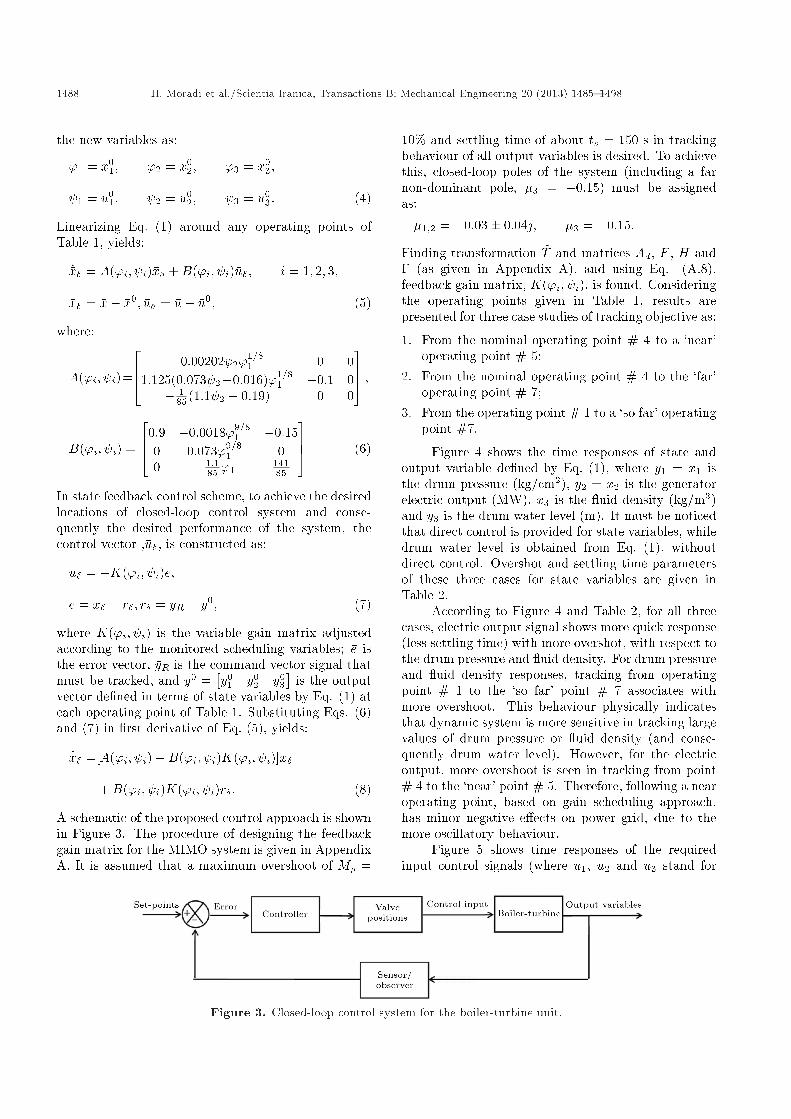
A schematic of the proposed control approach is shownin Figure 3. The procedure of designing the feedbackgain matrix for the MIMO system is given in AppendixA. It is assumed that a maximum overshoot of Mp =

10% and settling time of about ts = 150 s in trackingbehaviour of all output variables is desired. To achievethis, closed-loop poles of the system (including a farnon-dominant pole, �3 = �0:15) must be assignedas:

�1;2 = �0:03� 0:04j; �3 = �0:15:

Finding transformation ~T and matrices Ad, F , H and� (as given in Appendix A), and using Eq. (A.8),feedback gain matrix, K('i; i), is found. Consideringthe operating points given in Table 1, results arepresented for three case studies of tracking objective as:

1. From the nominal operating point # 4 to a `near'operating point # 5;

2. From the nominal operating point # 4 to the `far'operating point # 7;

3. From the operating point # 1 to a `so far' operatingpoint #7.

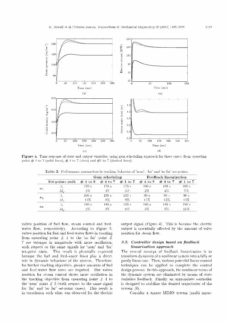
Figure 4 shows the time responses of state andoutput variable de�ned by Eq. (1), where y1 = x1 isthe drum pressure (kg/cm2), y2 = x2 is the generatorelectric output (MW), x3 is the uid density (kg/m3)and y3 is the drum water level (m). It must be noticedthat direct control is provided for state variables, whiledrum water level is obtained from Eq. (1), withoutdirect control. Overshot and settling time parametersof these three cases for state variables are given inTable 2.

According to Figure 4 and Table 2, for all threecases, electric output signal shows more quick response(less settling time) with more overshot, with respect tothe drum pressure and uid density. For drum pressureand uid density responses, tracking from operatingpoint # 1 to the `so far' point # 7 associates withmore overshoot. This behaviour physically indicatesthat dynamic system is more sensitive in tracking largevalues of drum pressure or uid density (and conse-quently drum water level). However, for the electricoutput, more overshoot is seen in tracking from point# 4 to the `near' point # 5. Therefore, following a nearoperating point, based on gain scheduling approach,has minor negative e�ects on power grid, due to themore oscillatory behaviour.

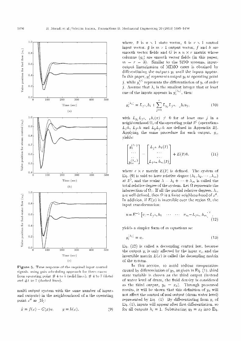
Figure 5 shows time responses of the requiredinput control signals (where u1, u2 and u3 stand for

Figure 3. Closed-loop control system for the boiler-turbine unit.


Figure 4. Time response of state and output variables, using gain scheduling approach for three cases: from operatingpoint # 4 to 5 (solid lines), # 4 to 7 (dots) and #1 to 7 (dashed lines).

Table 2. Performance parameters in tracking behavior of `near', `far' and `so far' set-points.

Gain scheduling Feedback linearizationSet-points path # 4 to 5 # 4 to 7 # 1 to 7 # 4 to 5 # 4 to 7 # 1 to 7

x1ts 170 s 170 s 170 s 100 s 100 s 100 sMp 2% 3% 5% 2% 4% 7%

x2ts 100 s 100 s 100 s 90 s 90 s 90 sMp 15% 8% 9% 17% 13% 15%

x3ts 180 s 180 s 180 s 180 s 180 s 180 sMp 2% 3% 6% 3% 5% 11%

valves position of fuel ow, steam control and feed-water ow, respectively). According to Figure 5,valves position for fuel and feed-water ows in trackingfrom operating point # 1 to the `so far' point #7 are stronger in magnitude with more oscillation,with respect to the same signals for `near' and `far'set-point cases. This result is physically expectedbecause the fuel and feed-water ows play a directrole in dynamic behaviour of the system. Therefore,for further tracking objectives, greater amounts of fueland feed-water ow rates are required. But valvesposition for steam control shows more oscillation inthe tracking objective from operating point # 4 tothe `near' point # 5 (with respect to the same signalfor `far' and `so far' set-point cases). This result isin correlation with what was observed for the electric

output signal (Figure 4). This is because the electricoutput is essentially a�ected by the amount of valveposition for steam ow.

3.2. Controller design based on feedbacklinearization approach

The central concept of feedback linearization is totransform dynamics of a nonlinear system into a fully orpartly linear one. Then, various powerful linear controltechniques can be applied to complete the controldesign process. In this approach, the nonlinear terms ofthe dynamic system are eliminated by means of statevariables feedback. Finally, an appropriate controlleris designed to stabilize the desired trajectories of thesystem [35].

Consider a square MIMO system (multi input-


Figure 5. Time response of the required input controlsignals, using gain scheduling approach for three cases:from operating point # 4 to 5 (solid lines), # 4 to 7 (dots)and #1 to 7 (dashed lines).

multi output system with the same number of inputsand outputs) in the neighbourhood of a the operatingpoint �x0 as [35]:

_�x = f(�x) +G(�x)�n; �y = h(�x); (9)

where, �x is n � 1 state vector, �u is r � 1 controlinput vector, �y is m � 1 output vector, f and h aresmooth vector �elds and G is a n � r matrix whosecolumns (gi) are smooth vector �elds (in this paper,m = r = 3). Similar to the SISO systems, input-output linearization of MIMO cases is obtained bydi�erentiating the outputs yi until the inputs appear.In this paper, yji represents output yi at operating pointj, while y(j)

i represents the di�erentiation of yi of orderj. Assume that �i is the smallest integer that at leastone of the inputs appears in y(�i)

i , then:

y(�i)i = Lf�ihi +

rXj=1

LgjLf�i�1hiuj ; (10)

with LgjLf�i�1hi(x) 6= 0 for at least one j in aneighbourhood i of the operating point �x0 (operationsLfh, Lfih and LgLfih are de�ned in Appendix B).Applying the same procedure for each output, yi,yields:2664y

(�1)1: : :: : :y(�m)m

3775 =

2664 Lf�1h1(�x): : :: : :

Lf�mhm(�x)

3775+ E(�x)�u; (11)

where r � r matrix E(�x) is de�ned. The system ofEq. (9) is said to have relative degree (�1; �2; � � � ; �m)at �x0, and the scalar � = �1 + � � � + �m is called thetotal relative degree of the system. Let represents theintersection of i. If all the partial relative degrees, �i,are well de�ned, then is a �nite neighbourhood of �x0.In addition, if E(�x) is invertible over the region , theinput transformation:

�u=E�1 �v1�Lf�1h1 � � � � � � vm�Lf�mhm�T ;(12)

yields a simpler form of m equations as:

y(�i)i = vi: (13)

Eq. (12) is called a decoupling control law, becausethe output yi is only a�ected by the input vi, and theinvertible matrix E(�x) is called the decoupling matrixof the system.

In this section, to avoid tedious computationcaused by di�erentiation of y3, as given in Eq. (1), thirdstate variable is chosen as the third output (insteadof water level of drum, the uid density is consideredas the third output, y3 = x3). Through presentedresults, it will be shown that this de�nition of y3 willnot a�ect the control of real output (drum water level)represented by Eq. (1). By di�erentiating from yi ofEq. (1), inputs will appear after �rst di�erentiation, sofor all outputs �i = 1. Substituting y3 = x3 into Eq.


(1), and di�erentiating from it, yields:264y(1)1

y(1)2

y(1)3

375 =

24 0�0:1x2 � 0:016x9=8

10:1985 x1

35+

2640:9 �0:0018x9=81 �0:15

0 0:073x9=81 0

0 � 1:185 x1

14185

375 �u: (14)

According to Eq. (12), control signal �u is constructedas:

�u = E�1

24 v1

v2 + 0:1x2 + 0:016x9=81

v3 � 0:1985 x1

35 ; (15)

where:

E =

240:9 �0:0018x19=8 �0:15

0 0:073x9=81 0

0 � 1:185 x1

14185

35 : (16)

Using this control law results in three separate dynam-ics for three outputs as:

y(1)i = vi; i = 1; 2; ; 3: (17)

After decoupling the outputs dynamics, a PI controlleris designed as:

vi = �K1iei �K2i�i; _�i = ei = yi � ri; (18)

where ri is the command input signal that is desired tobe tracked. Di�erentiating from Eq. (17) yields:

�yi +K1i _yi +K2iyi = K1i _ri +K2iri: (19)

Transforming this equation into the Laplace domain,yields:

Yi(s)Ri(s)

=K1is+K2i

s2 +K1is+K2i: (20)

If the closed loop system is expected to have abehaviour similar to the system with the followingcharacteristic equation:

s2 + 2�!ns+ !2n = 0; !n > 0; 0 < � < 1;

(21)

control gains must be adjusted as:

K1i = 2�i!i;

K2i = !2i : (22)

Again, to have a maximum overshoot of Mp = 10% andsettling time of about ts = 150 s in tracking behaviour

of all output variables, parameters of Eq. (22) must beselected as !i = 0:05, �i = 0:6, i = 1; 2; 3.

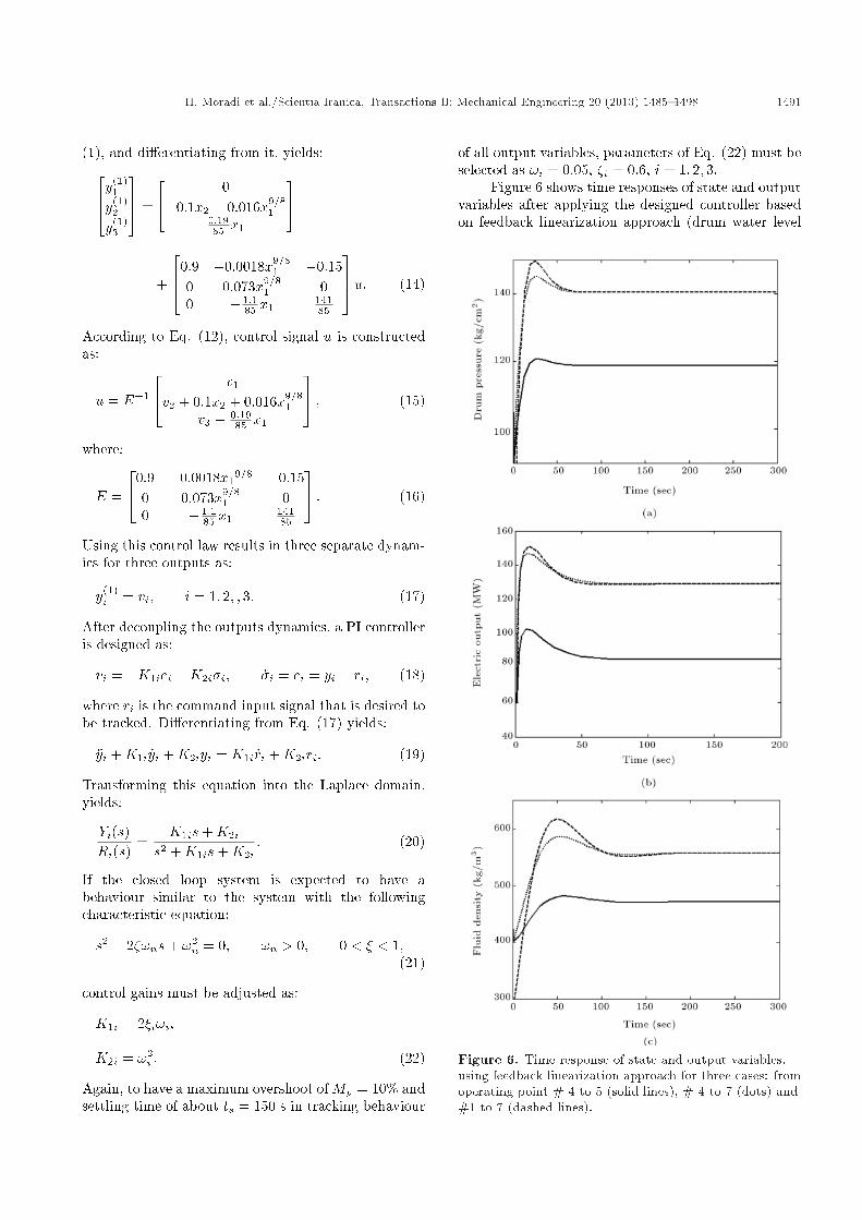
Figure 6 shows time responses of state and outputvariables after applying the designed controller basedon feedback linearization approach (drum water level

Figure 6. Time response of state and output variables,using feedback linearization approach for three cases: fromoperating point # 4 to 5 (solid lines), # 4 to 7 (dots) and#1 to 7 (dashed lines).


shows a similar behaviour as given in Figure 4(d).Overshot and settling time parameters of these threecases for state variables is given in Table 2. Accordingto Figure 6 and Table 2, electric output behaviourshows more quick response (less settling time) withmore overshoot, with respect to the drum pressure and uid density for all three cases. For electric outputresponse, tracking from operating point # 4 to the`near' point # 5 associates with more overshoot, whilefor the drum pressure and uid density, more overshootis seen in tracking from point # 1 to the `so far'point # 7. Therefore, for both control approaches(Figures 4 and 6), dynamic system is more sensitivein tracking of larger values of drum pressure or uiddensity, and in tracking of closer values of electricoutput.

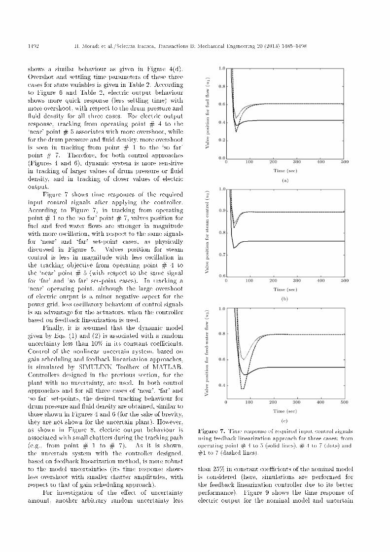
Figure 7 shows time responses of the requiredinput control signals after applying the controller.According to Figure 7, in tracking from operatingpoint # 1 to the `so far' point # 7, valves position forfuel and feed-water ows are stronger in magnitudewith more oscillation, with respect to the same signalsfor `near' and `far' set-point cases, as physicallydiscussed in Figure 5. Valves position for steamcontrol is less in magnitude with less oscillation inthe tracking objective from operating point # 4 tothe `near' point # 5 (with respect to the same signalfor `far' and `so far' set-point cases). In tracking a`near' operating point, although the large overshootof electric output is a minor negative aspect for thepower grid, less oscillatory behaviour of control signalsis an advantage for the actuators, when the controllerbased on feedback linearization is used.

Finally, it is assumed that the dynamic modelgiven by Eqs. (1) and (2) is associated with a randomuncertainty less than 10% in its constant coe�cients.Control of the nonlinear uncertain system, based ongain scheduling and feedback linearization approaches,is simulated by SIMULINK Toolbox of MATLAB.Controllers designed in the previous section, for theplant with no uncertainty, are used. In both controlapproaches and for all three cases of `near', `far' and`so far' set-points, the desired tracking behaviour fordrum pressure and uid density are obtained, similar tothose shown in Figures 4 and 6 (for the sake of brevity,they are not shown for the uncertain plant). However,as shown in Figure 8, electric output behaviour isassociated with small chatters during the tracking path(e.g., from point # 1 to # 7). As it is shown,the uncertain system with the controller designed,based on feedback linearization method, is more robustto the model uncertainties (its time response showsless overshoot with smaller chatter amplitudes, withrespect to that of gain scheduling approach).

For investigation of the e�ect of uncertaintyamount, another arbitrary random uncertainty less

Figure 7. Time response of required input control signalsusing feedback linearization approach for three cases: fromoperating point # 4 to 5 (solid lines), # 4 to 7 (dots) and#1 to 7 (dashed lines).

than 25% in constant coe�cients of the nominal modelis considered (here, simulations are performed forthe feedback linearization controller due to its betterperformance). Figure 9 shows the time response ofelectric output for the nominal model and uncertain


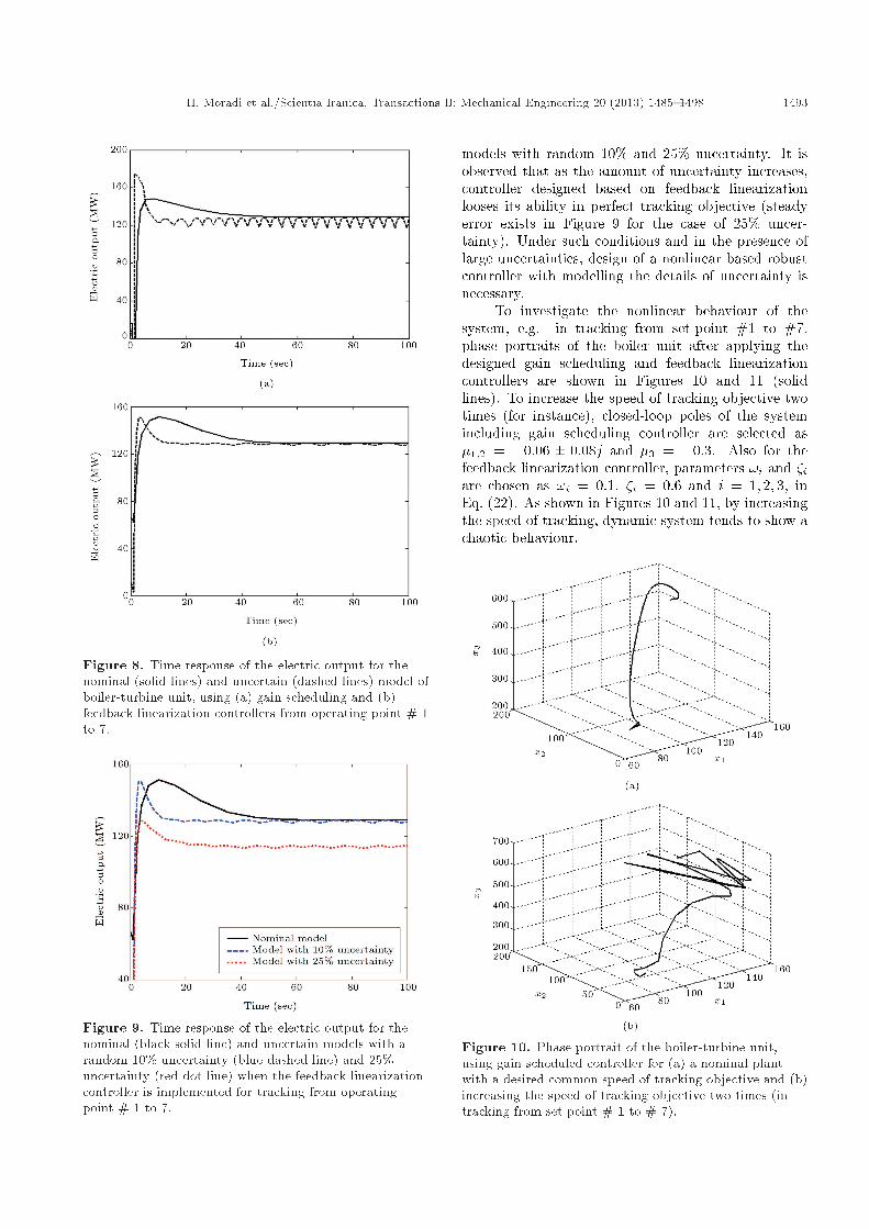
Figure 8. Time response of the electric output for thenominal (solid lines) and uncertain (dashed lines) model ofboiler-turbine unit, using (a) gain scheduling and (b)feedback linearization controllers from operating point # 1to 7.

Figure 9. Time response of the electric output for thenominal (black solid line) and uncertain models with arandom 10% uncertainty (blue dashed line) and 25%uncertainty (red dot line) when the feedback linearizationcontroller is implemented for tracking from operatingpoint # 1 to 7.

models with random 10% and 25% uncertainty. It isobserved that as the amount of uncertainty increases,controller designed based on feedback linearizationlooses its ability in perfect tracking objective (steadyerror exists in Figure 9 for the case of 25% uncer-tainty). Under such conditions and in the presence oflarge uncertainties, design of a nonlinear based robustcontroller with modelling the details of uncertainty isnecessary.

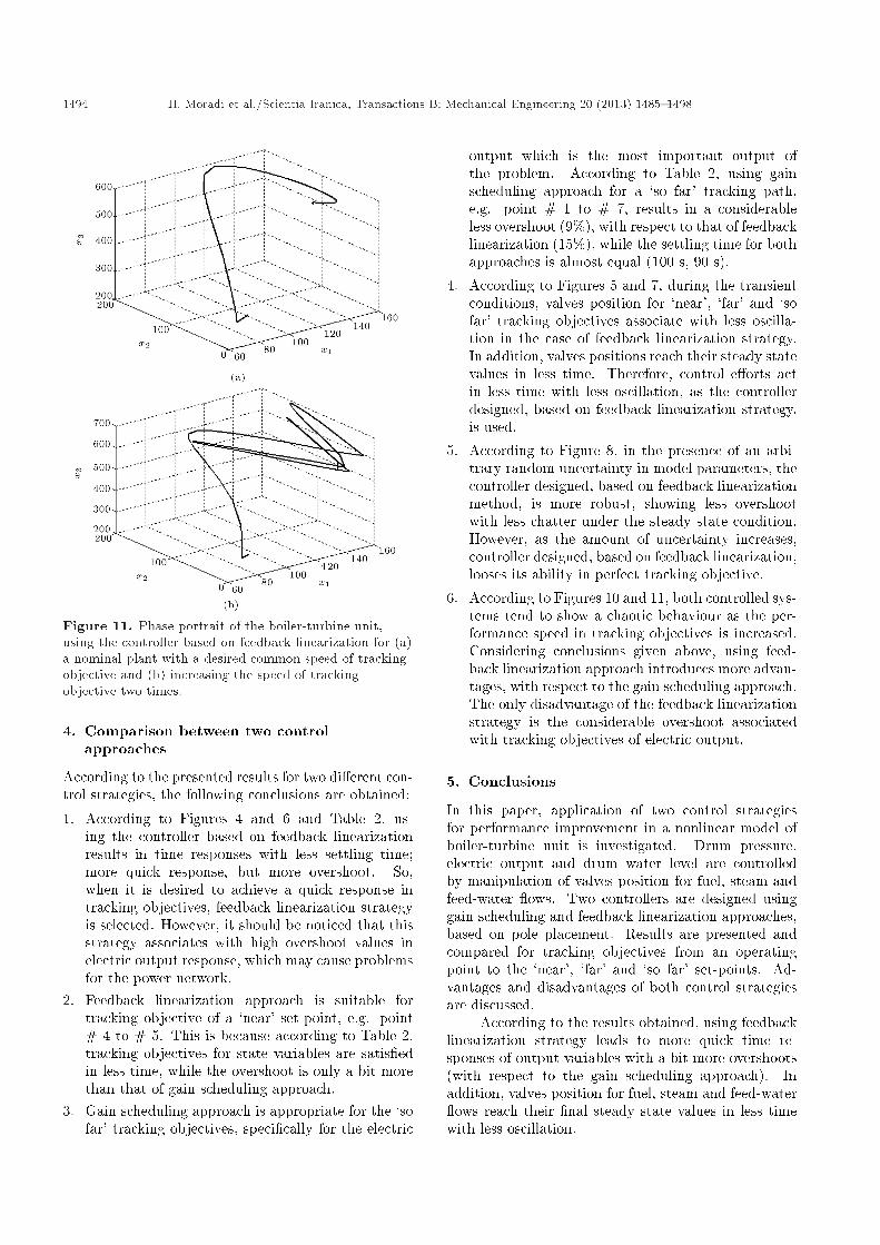
To investigate the nonlinear behaviour of thesystem, e.g. in tracking from set-point #1 to #7,phase portraits of the boiler unit after applying thedesigned gain scheduling and feedback linearizationcontrollers are shown in Figures 10 and 11 (solidlines). To increase the speed of tracking objective twotimes (for instance), closed-loop poles of the systemincluding gain scheduling controller are selected as�1;2 = �0:06 � 0:08j and �3 = �0:3. Also for thefeedback linearization controller, parameters !i and �iare chosen as !i = 0:1, �i = 0:6 and i = 1; 2; 3, inEq. (22). As shown in Figures 10 and 11, by increasingthe speed of tracking, dynamic system tends to show achaotic behaviour.

Figure 10. Phase portrait of the boiler-turbine unit,using gain scheduled controller for (a) a nominal plantwith a desired common speed of tracking objective and (b)increasing the speed of tracking objective two times (intracking from set-point # 1 to # 7).


Figure 11. Phase portrait of the boiler-turbine unit,using the controller based on feedback linearization for (a)a nominal plant with a desired common speed of trackingobjective and (b) increasing the speed of trackingobjective two times.

4. Comparison between two controlapproaches

According to the presented results for two di�erent con-trol strategies, the following conclusions are obtained:

1. According to Figures 4 and 6 and Table 2, us-ing the controller based on feedback linearizationresults in time responses with less settling time;more quick response, but more overshoot. So,when it is desired to achieve a quick response intracking objectives, feedback linearization strategyis selected. However, it should be noticed that thisstrategy associates with high overshoot values inelectric output response, which may cause problemsfor the power network.

2. Feedback linearization approach is suitable fortracking objective of a `near' set-point, e.g. point# 4 to # 5. This is because according to Table 2,tracking objectives for state variables are satis�edin less time, while the overshoot is only a bit morethan that of gain scheduling approach.

3. Gain scheduling approach is appropriate for the `sofar' tracking objectives, speci�cally for the electric

output which is the most important output ofthe problem. According to Table 2, using gainscheduling approach for a `so far' tracking path,e.g. point # 1 to # 7, results in a considerableless overshoot (9%), with respect to that of feedbacklinearization (15%), while the settling time for bothapproaches is almost equal (100 s, 90 s).

4. According to Figures 5 and 7, during the transientconditions, valves position for `near', `far' and `sofar' tracking objectives associate with less oscilla-tion in the case of feedback linearization strategy.In addition, valves positions reach their steady statevalues in less time. Therefore, control e�orts actin less time with less oscillation, as the controllerdesigned, based on feedback linearization strategy,is used.

5. According to Figure 8, in the presence of an arbi-trary random uncertainty in model parameters, thecontroller designed, based on feedback linearizationmethod, is more robust, showing less overshootwith less chatter under the steady state condition.However, as the amount of uncertainty increases,controller designed, based on feedback linearization,looses its ability in perfect tracking objective.

6. According to Figures 10 and 11, both controlled sys-tems tend to show a chaotic behaviour as the per-formance speed in tracking objectives is increased.Considering conclusions given above, using feed-back linearization approach introduces more advan-tages, with respect to the gain scheduling approach.The only disadvantage of the feedback linearizationstrategy is the considerable overshoot associatedwith tracking objectives of electric output.

5. Conclusions

In this paper, application of two control strategiesfor performance improvement in a nonlinear model ofboiler-turbine unit is investigated. Drum pressure,electric output and drum water level are controlledby manipulation of valves position for fuel, steam andfeed-water ows. Two controllers are designed usinggain scheduling and feedback linearization approaches,based on pole placement. Results are presented andcompared for tracking objectives from an operatingpoint to the `near', `far' and `so far' set-points. Ad-vantages and disadvantages of both control strategiesare discussed.

According to the results obtained, using feedbacklinearization strategy leads to more quick time re-sponses of output variables with a bit more overshoots(with respect to the gain scheduling approach). Inaddition, valves position for fuel, steam and feed-water ows reach their �nal steady state values in less timewith less oscillation.


In the presence of an arbitrary parametric un-certainty in the nonlinear model, the desired trackingobjectives are achieved for output variables in bothmethods. However, for the controller designed basedon gain scheduling approach, electric output signal isassociated with considerable oscillations. This problemcan be solved by decreasing the speed of tracking set-points. Finally, a chaotic behaviour of the boiler-turbine unit is seen when the speed of tracking pro-cess is increased. In future, to improve the robustperformance of such MIMO systems against possibleuncertainties, a nonlinear-based robust controller canbe developed.

Acknowledgments

This research has been supported by the `National EliteFoundation' of Iran.

References

1. Tan, W., Marquez, H.J., Chen, T. and Liu, J. \Anal-ysis and control of a nonlinear boiler-turbine unit", J.of Proc. Control, 15, pp. 883-891 (2005).

2. Tan, W., Fang, F., Tian, L., Fu, C. and Liu, J. \Linearcontrol of a boiler-turbine unit: Analysis and design",ISA Trans., 47, pp. 189-197 (2008).

3. Astrom, K.J. and Eklund, K. \A simpli�ed nonlinearmodel of a drum boiler turbine unit", Int. J. of Control,16(1), pp. 145-169 (1972).

4. Bell, R.D. and Astrom, K.J. \Dynamic models forboiler-turbine-alternator units: Data logs and pa-rameter estimation for a 160 MW unit", Tech. Rep.Report LUTFD2/(TFRT-3192)/1-137; Department ofAutomatic Control, Lund Inst. of Tech., Lund, Sweden(1987).

5. Lo, K.L., Zeng, P.L., Marchand, E. and Pinkerton,A. \Modelling and state estimation of power plantsteam turbines", IEEE Proc., Part C, 137(2), pp. 80-94 (1990).

6. Murty, V.V., Sreedhar, R., Fernandez, B., Masada,G.Y. and Hill, A.S. \Boiler system identi�cation us-ing sparse neural networks", Proc. of ASME WinterMeeting, New Orleans, pp. 103-111 (1993).

7. Donate, P.D. and Moiola, J.L. \Model of a once-through boiler for dynamic studies", Latin AmericanApplied Research, 24, pp. 159-166 (1994).

8. Rink, R., White, D., Chiu, A. and Leung, R. \SYN-SIM: A computer simulation model for the Mildredlake steam/electrical system of syncrude Canada Ltd",Technical report, Univ. Alberta, Edmonton, AB,Canada (1996).

9. Adam, E.J. and Marchetti, J.L. \Dynamic simulationof large boilers with natural recirculation", J. of Comp.& Chem. Eng., 23, pp. 1031-1040 (1999).

10. Kim, H. and Choi, S. \A model on water leveldynamics in natural circulation drum-type boilers",Int. Comm. in Heat & Mass Trans., 32, pp. 786-796(2005).

11. Lu, S. and Hogg, B.W. \Dynamic nonlinear modellingof power plant by physical principles and neural net-works", J. of Elec. Power & Energy Sys., 22, pp. 67-78(2000).

12. McDonald, J.P., Kwatny, G.H. and Spare, J.H. \Anonlinear model for reheat boiler-turbine generationsystems", Proc. JACC, pp. 227-236 (1971).

13. Bell, R.D. and Astrom, K.J. \A fourth order non-linearmodel for drum-boiler dynamics", IFAC '96, Preprints13th World Congress of IFAC, O, San Francisco, pp.31-36 (1996).

14. Astrom, K.J. and Bell, R.D. \Drum-boiler dynamics",J. of Automatica, 36, pp. 363-378 (2000).

15. McDonald, J.P. and Kwatny, H.G. \Design and anal-ysis of boiler-turbine-generator controls using linearoptimal regulator theory", IEEE Trans. Auto. Control,AC-18, pp. 202-209 (1973).

16. Corit, R. and Ma�ezzoni, C. \Practical-optimal con-trol of a drum boiler power plant", J. of Automatica,20(2), pp. 163-173 (1984).

17. Borsi, L. \Design and experimental evaluation ofdecoupling control for a boiler turbine unit", Modellingand Control Seminar, Sidney (1977).

18. Prasad, G., Swidenbank, E. and Hogg, B.W. \Alocal model networks based multivariable long-rangepredictive control strategy for thermal power plants",J. of Automatica, 34(10), pp. 1185-1204 (1998).

19. Prokhorenkov, A.M. and Sovlukov, A.S. \Fuzzy mod-els in control systems of boiler aggregate technologicalprocesses", J. of Comp. Stand. & Interf., 24, pp. 151-159 (2002).

20. Kocaarslan, I., Ertu�grul, C. and Tiryaki, H. \A fuzzylogic controller application for thermal power plants",J. of Energy Conv. & Manag., 47, pp. 442-458 (2006).

21. Liu, X.J., Lara-Rosanoa, F. and Chan, C.W. \Neuro-fuzzy networkmodelling and control of steam pressurein 300MW steam-boiler system", J. of Eng. App. ofArtif. Intel., 16, pp. 431-440 (2003).

22. Eitelberg, E. and Boje, E. \Water circulation controlduring once-through boiler start-up", J. of ControlEng. Prac., 12, pp. 677-685 (2004).

23. Li, D., Chen, T., Marquez, H.J. and Gooden, R.K.\Life extending control of boiler-turbine systems viamodel predictive methods", J. of Control Eng. Prac.,14, pp. 319-326 (2006).

24. Chen, P.C. and Shamma, J.S. \Gain-scheduled-optimal control for boiler-turbine dynamics with ac-tuator saturation", Int. J. of Proc. Control, 14, pp.263-277 (2004).

25. Yu, T., Chan, K.W., Tong, J.P., Zhou, B. and Li,D.H. \Coordinated robust nonlinear boiler-turbine-generator control systems via approximate dynamic


feedback linearization", J. of Proc. Control, 20, pp.365-374 (2010).

26. Abdennour, A. \An intelligent supervisory system fordrum type boilers during severe disturbances", J. ofElec. Power & Energy Syst., 22, pp. 381-387 (2000).

27. Nanhua, Y., Wentong, M. and Ming, S. \Applicationof adaptive Gray predictor based algorithm to boilerdrum level control", J. of Energy Conv. & Manag., 47,pp. 2999-3007 (2006).

28. Fang, F. and Wei, L. \Backstepping-based nonlinearadaptive control for coal-�red utility boiler-turbineunits", J. of App. Energy, 88, pp. 814-824 (2011).

29. Moradi, H., Bakhtiari-Nejad, F. and Sa�ar-Avval,M. \Robust control of an industrial boiler system; acomparison between two approaches: Sliding modecontrol & technique", J. of Energy Conv. & Manag.,50, pp. 1401-1410 (2009).

30. Pellegrinetti, G. and Bentsman, J. \Controller designfor boilers", Int. J. of Robust Nonl. Control, 4, pp.645-671 (1994).

31. Tan, W., Marquez, H.J. and Chen, T. \Multivariablerobust controller design for a boiler system", IEEETrans. of Control Syst. Tech., 10(5), pp. 735-742(2002).

32. Moradi, H., Sa�ar-Avval, M. and Bakhtiari-Nejad,F. \Sliding mode control of drum water level in anindustrial boiler unit with time varying parameters: Acomparison with H-in�nity robust control approach",J. of Proc. Control, 22(10), pp. 1844-1855 (2012).

33. Moradi, H., Bakhtiari-Nejad, F., Sa�ar-Avval, M. andAlasty, A. \Using sliding mode control to adjust drumlevel of a boiler unit with time varying parameters",ASME 2010 10th Biennial Conf. on Eng. Sys. Des. &Anal., ESDA2010-24105, July 12-14, Istanbul, Turkey(2010).

34. Khalil, H.K., Nonlinear Systems, 2nd Edn., PrenticeHall Inc., Upper Saddle River, NJ (1996).

35. Slotine, J.J. and Li, W., Applied Nonlinear Control,Prentice Hall Inc., Englewood Cli�s, NJ (1991).

36. D' Azzo, J. and Houpis, H., Linear Control SystemAnalysis and Design: Conventional and Modern, 4thEdn., McGraw-Hill, New York (1995).

Appendix A

Dynamic model of boiler-turbine unit is of rank n = 3.Since the controllability matrix:

�c =�B AB A2B � � �An�1B

�;

is of rank 3, dynamic system is completely statecontrollable. Using the similarity transformation ~T as�x = ~T �z, Eq. (5) is represented as:

_�z� = AG�z� + BG�u�

AG = ~T�1AT; BG = ~T�1B; (A.1)

where �z� is the new introduced state vector. Also, usingthe following transformations:

�u� = F �w�; �w� = �v� �H�z�: (A.2)

Eq. (A.1) is described as:

_�z� = AG�z� +BG�v�;

AG = AG � BGFH; BG = BGF; (A.3)

where �v� is the new control input vector and AG,BG have the general canonical form with elementsof [Ai] i� i ; [Bi] i�1; i = 1; 2; ::; r and

Pri=1 i = n

as [36]:

AG =

2664[A1] 0 � � � 00 [A2] � � � 0

:0 0 � � � [Ar]

3775n�n

;

BG =

2664[B1] 0 � � � 00 [B2] � � � 0

:0 0 � � � [Br]

3775n�r

;

[Ai] =

2666640 1 0 � � � 00 0 1 � � � 0

:0 0 0 � � � 10 0 0 � � � 0

377775 i� i

;

[Bi] =

26666400::1

377775 i�1

; (A.4)

where r is the number of input variables (in this case,r = 3). Introducing the modi�ed controllability matrixas:

��c =hb1 b2 � � � br

...

Ab1 Ab2 � � � Abr... � � � ...

An�rb1 An�rb2 � � � An�rbr�;

where bi are the columns of matrix B given in Eq. (5).A regular basis of ��c is developed as

�c =hb1 Ab1 � � � A 1�1b1

...

b2 Ab2 � � � A 2�1b2... � � � ...

br Abr � � � A r�1br�; (A.5)


where each column, Ajbi, i = 1; � � � ; r, j = 0; � � � ; r, isindependent from its previous columns. Inverse of �cgiven by Eq. (A.5) is displayed as (all of the paper, [ ]0stands for transpose of the [ ] quantity):

��1c =

he011 � � � e01 1

...

e021 � � � e02 2

... � � � ...

e0r1 � � � e0r r�0 :

Similarity transformation ~T is de�ned as [36]:

~T =�he01 1

e01 1A � � � e01 1

A 1�1 ...

e02 2e02 2

A � � � e02 2A 2�1 ... � � � ...

e0r r e0r rA � � � e0r r A r�1�0��1:

(A.6)

Considering again Eq. (A.3) and constructing thefeedback control law, as v� = ��z�, yields:

_�z� = Ad�z�; Ad = AG �BG�; (A.7)

where Ad is the desired state matrix including coef-�cients representing desired closed loop poles (jsI �Adj = (s� �1)(s� �2) � � � (s� �n)), having the generalform of AG as given by Eq. (A.4). Considering Eqs.(7) and (A.2) and similarity transformation �x� = ~T �z�,yields the feedback control law of the system as:

�u� = �K('i; i)�x�;

K('i; i) = F [� +H] ~T�1; (A.8)

where F , H and � are obtained using Eqs. (A.2), (A.3)and (A.7) as follows:

F = (B0GBG)�1; H = B0G(AG � AG);

� = B0G(AG �Ad): (A9)

Appendix B

Lie derivative de�nitionLet h : Rn ! R be a smooth scalar function and f :Rn ! R be a smooth vector �eld on Rn. The Liederivative of h with respect to f is a scalar functionde�ned by [35]:

Lfh = rh:f:Repeated Lie derivatives can be de�ned recursively as:

Lf0h = h; Lfih = Lf (Lfi�1h) = r(Lfi�1h):f:

Similarly, if g is another vector �eld, then the scalarfunction LgLfh(x) is:

LgLfh = r(Lfh):g:

Biographies

Hamed Moradi was born in Isfahan in 1984. Hereceived his BS degree in Mechanical Engineering inSolid Mechanics from Amirkabir University of Technol-ogy, in 2005; his MS and PhD degrees in MechanicalEngineering in Applied Mechanics from Sharif Univer-sity of Technology (SUT), Tehran, Iran, in 2008 and2012, respectively. Currently he is the post-doctoralassociate in SUT, working on optimal nonlinear controlof process in mechanical systems & installations toreduce energy consumption. During 2008-2012 he hasbeen an invited faculty member in the Department ofMechanical Engineering, Hormozgan National Univer-sity, Bandar-Abbas, Iran.

His current research interests include modeling ofdynamic systems, application of robust, nonlinear andoptimal control methods in various dynamics systemssuch as manufacturing, bio-engineering, thermo- uidindustrial processes and power plant engineering. Also,he currently investigates the analysis of nonlineardynamics and chaos in various oscillatory phenomena,and especially in two areas of thermo- uid systems andmachining chatter vibrations.

Aria Alasty received his BSc and MSc degrees inMechanical Engineering from Sharif University of Tech-nology (SUT), Tehran, Iran, in 1987 and 1989. He alsoreceived his Ph.D. degree in Mechanical Engineeringfrom Carleton University, Ottawa, Canada, in 1996. Atpresent, he is a Professor in Mechanical Engineeringin Sharif University of Technology. He has been amember of Center of Excellence in Design, Robotics,and Automation (CEDRA) since 2001. His �elds ofresearch are mainly in nonlinear and chaotic systemscontrol, computational nano/micro mechanics and con-trol, special purpose robotics, robotic swarm controland fuzzy system control.

Majid Sa�ar-Avval is Professor of Mechanical Engi-neering at Amirkabir University of Technology (AUT),Tehran, Iran. He received his BSc and MSc degreesfrom Sharif University of Technology, and his Ph.D.degree from the Ecole Nationale des Arts et Metiers(ENSAM), Paris, in 1985. He has been teaching atthe AUT since then. He was head of MechanicalEngineering Department from June 2000 to June 2002,and has been head of `Energy and Control Center ofExcellence', from May 2007 to March 2012 at AUT.His research contributions are in the �eld of twophase heat transfer, advanced thermal systems, energymanagement and bio-heat transfer.

Firooz Bakhtiari-Nejad was born in Iran in 1951.He received his BS degree in Electrical Engineeringand Mechanical Engineering, his MS degree in Me-


chanical Engineering and PhD degree in MechanicalEngineering from Kansas State University, USA in1975, 1978 and 1983, respectively. He was AssistantProfessor in the Department of Mechanical Engineer-ing, Kerman University, Kerman, Iran, from 1983-1988, and Associate Professor from 1998 to 2004 andthen Professor of Mechanical Engineering from 2004 topresent at Amirkabir University of Technology (AUT),Tehran, Iran. He also was the director of research a�airand secretary general of centers of excellence console,

Ministry of Science, Research and Technology of Iranfrom 2005 to 2010.

His current research interests are the applicationof theoretical and experimental modal analysis for con-trol and health monitoring of systems and structures,digital control and adaptive optimal control of con-tinuous structures and multi variable systems such asinternal combustion engines and vehicle dynamics, andapplication of fuzzy and neural controls in mechanicalsystems.

Documents

Multivariable control of an industrial boiler-turbine unit with ...scientiairanica.sharif.edu/article_3406_f2afd3e6735ec841c70e77... · controllers based on LQG/LQR theory cannot