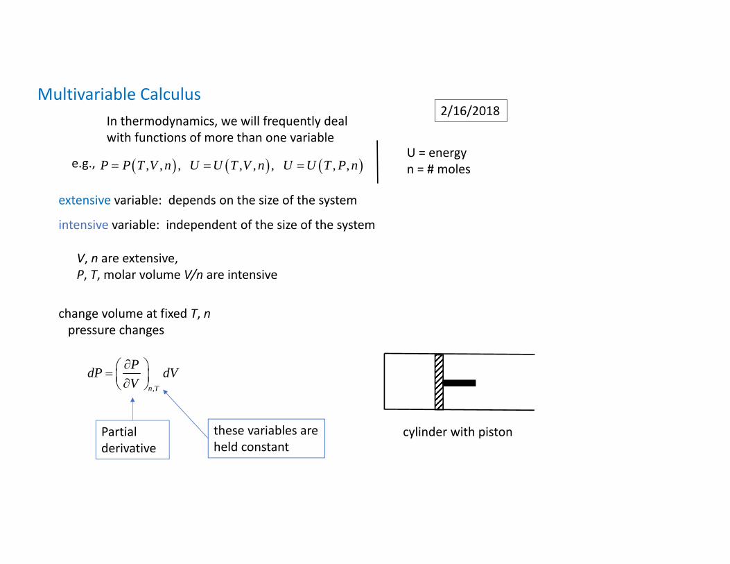
Multivariable CalculusIn thermodynamics, we will frequently dealwith functions of more than one variable

e.g., , , , , , , , , P P T V n U U T V n U U T P n

extensive variable:  depends on the size of the system

intensive variable:  independent of the size of the system

V, n are extensive, P, T, molar volume V/n are intensive

change volume at fixed T, npressure changes

,n T

PdP dVV

U = energyn = # moles

these variables areheld constant

cylinder with pistonPartial derivative

2/16/2018

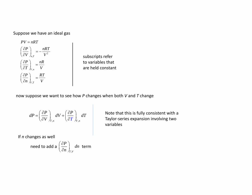
Suppose we have an ideal gas

2,

,

,

n T

V n

V T

PV nRTP nRTV V

P nRT V

P RTn V

subscripts referto variables thatare held constant

now suppose we want to see how P changes when both V and T change

, ,T n V n

P PdP dV TV T

d Note that this is fully consistent with a Taylor‐series expansion involving two variables

need to add a                    term,T V

P dnn

If n changes as well

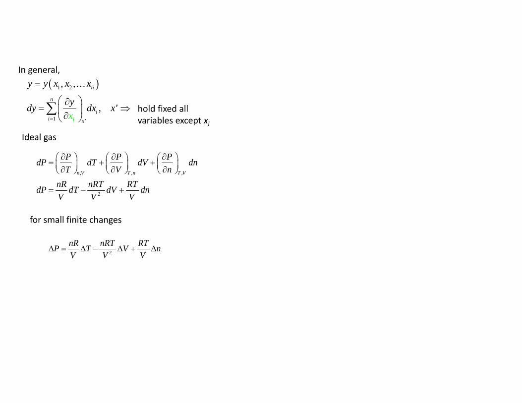
In general, 1 2

1

, ,

,

n

n

ii xi

y y x x x

ydyx

dx x

'

' hold fixed allvariables except xi

Ideal gas

, , ,

2

n V T n T V

P P PdP dT dV dnT V n

nR nRT RTdP dT dV dnV V V

for small finite changes

2

nR nRT RTP T V nV V V

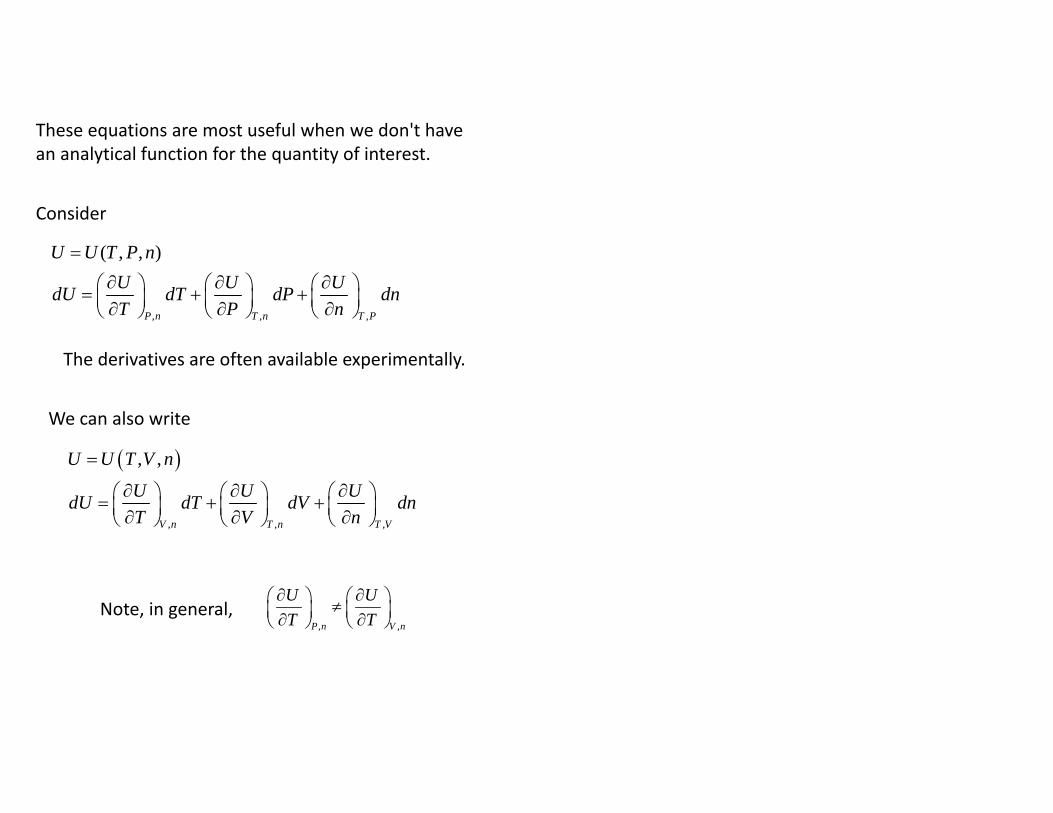
These equations are most useful when we don't havean analytical function for the quantity of interest.

, , ,

( , , )

P n T n T P

U U T P nU U UdU dT dP dnT P n

The derivatives are often available experimentally.

We can also write

, , ,

, ,

V n T n T V

U U T V n

U U UdU dT dV dnT V n

Note, in general,, ,P n V n

U UT T

Consider

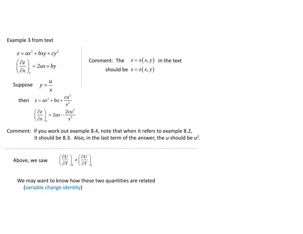
Example 3 from text

2 2

2y

z ax bxy cyz ax byx

Comment:  The                          in the text

,

,

z x x y

z z x y

should be

Suppose uyx

then2

22

2

3

22u

cuz ax bux

z cuaxx x

Above, we sawP V

U UT T

We may want to know how these two quantities are related(variable change identity)

Comment:  if you work out example 8.4, note that when it refers to example 8.2,it should be 8.3.  Also, in the last term of the answer, the u should be u2.

, , ,

, , ,

, , , , , ,

,

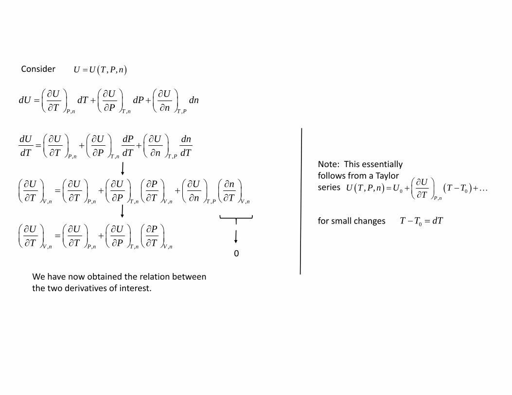
P n T n T P

P n T n T P

V n P n T n V n T P V n

V n

U U UdU dT dP dnT P n

dU U U dP U dndT T P dT n dT

U U U P U nT T P T n T

UT

, , ,P n T n V n

U U PT P T

0

, ,U U T P n

Note:  This essentiallyfollows from a Taylorseries 0 0

,

, ,P n

UU T P n U T TT

for small changes  0T T dT

Consider

We have now obtained the relation between the two derivatives of interest.

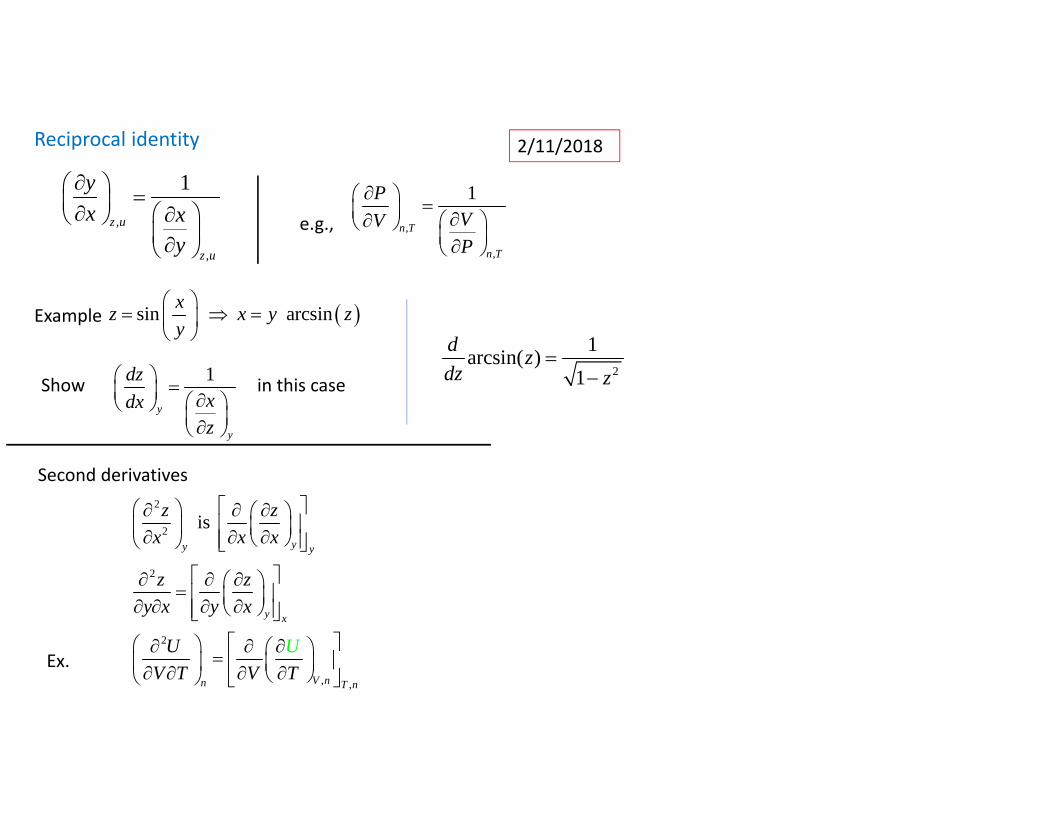
Reciprocal identity

,

,

1

z u

z u

yx x

y

e.g., ,

,

1

n T

n T

PVVP

Example sin arcsinxz x y zy

2

2

2

2

, ,

is yy y

y x

V nn T n

z zx x x

z zy x y x

UV T V T

U

Second derivatives

Show                                      in this case1

y

y

dzxdxz

Ex.

2

1arcsin( )1

d zdz z

2/11/2018

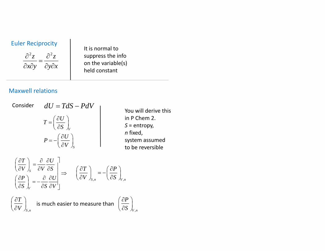
Euler Reciprocity2 2z z

x y y x

It is normal tosuppress the infoon the variable(s)held constant

Maxwell relations

Consider dU TdS PdV

V

S

UTS

UPV

You will derive thisin P Chem 2.S = entropy,n fixed,system assumed to be reversible

S

V

T UV V SP US S V

, ,S n V n

T PV S

, ,S n V n

T P V S

is much easier to measure than

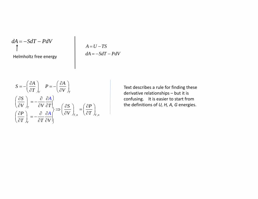
dA SdT PdV

Helmholtz free energy

, ,

V T

T

T n V n

V

A

A AS PT V

SV V T S P

V TPT

AT V

A U TSdA SdT PdV

Text describes a rule for finding these derivative relationships – but it is confusing.    It is easier to start from the definitions of U, H, A, G energies.

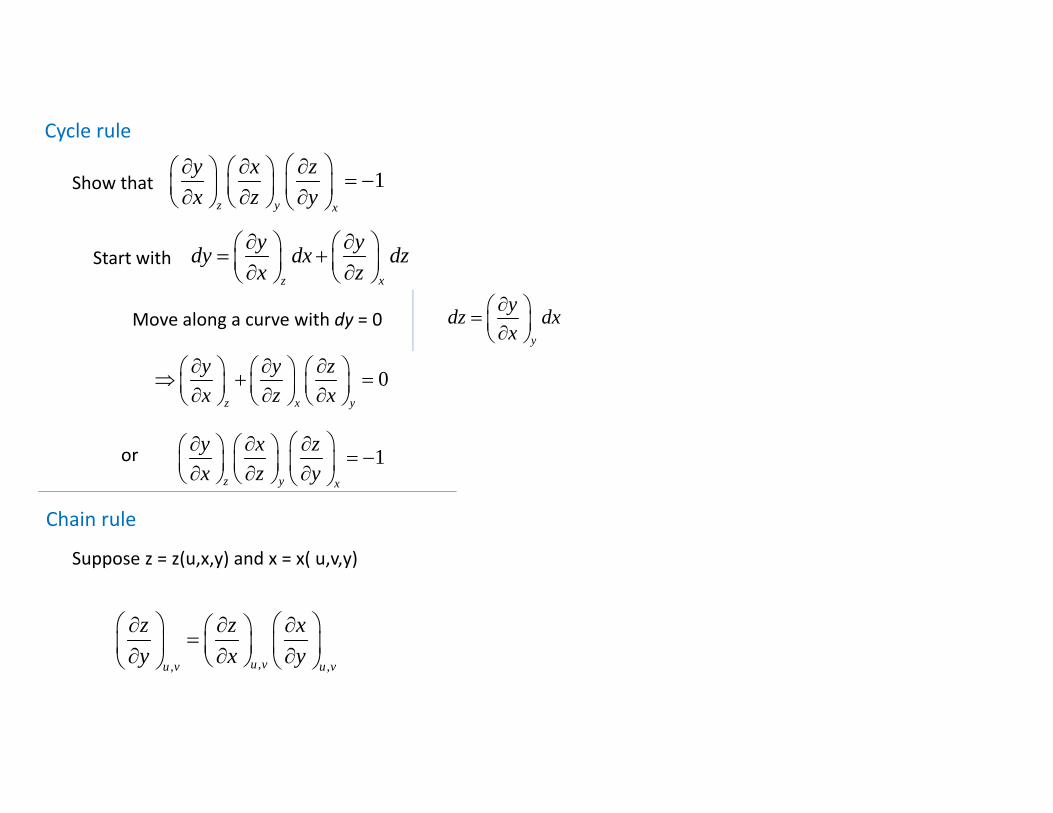
Cycle rule

1z y x

y x zx z y

Move along a curve with dy = 0

0z x y

y y zx z x

or 1z y x

y x zx z y

Chain rule

,, ,u vu v u v

z z xy x y

z x

y ydy dx dzx z

Show that

Start with

Suppose z = z(u,x,y) and x = x( u,v,y) 

y

ydz dxx

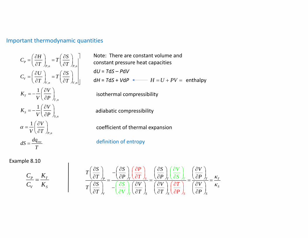
Important thermodynamic quantities

, ,

, ,

,

,

,

1

1

1

PP n P n

VV n V n

TT n

SS n

P n

rev

H SC TT T

U SC TT T

VKV P

VKV P

VV T

dqdST

Note:  There are constant volume and constant pressure heat capacitiesdU = TdS – PdVdH = TdS + VdP H U PV enthalpy

isothermal compressibility

adiabatic compressibility

definition of entropy

coefficient of thermal expansion

Example 8.10

P T

V S

C KC K

TP T

T

T T T

S

V S S

S

SS

SS S VTPT P P

S V V VTT T T

PT

TP

SP

VS

V

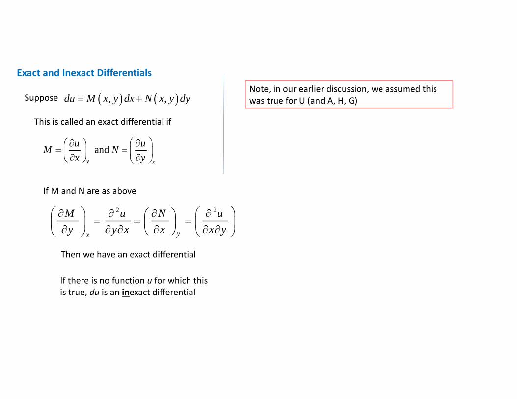
Exact and Inexact Differentials

Suppose , ,du M x y dx N x y dy

This is called an exact differential if

and y x

u uM Nx y

If there is no function u for which thisis true, du is an inexact differential

If M and N are as above

2 2

yx

M u N uy y x x x y

Then we have an exact differential

Note, in our earlier discussion, we assumed this was true for U (and A, H, G)

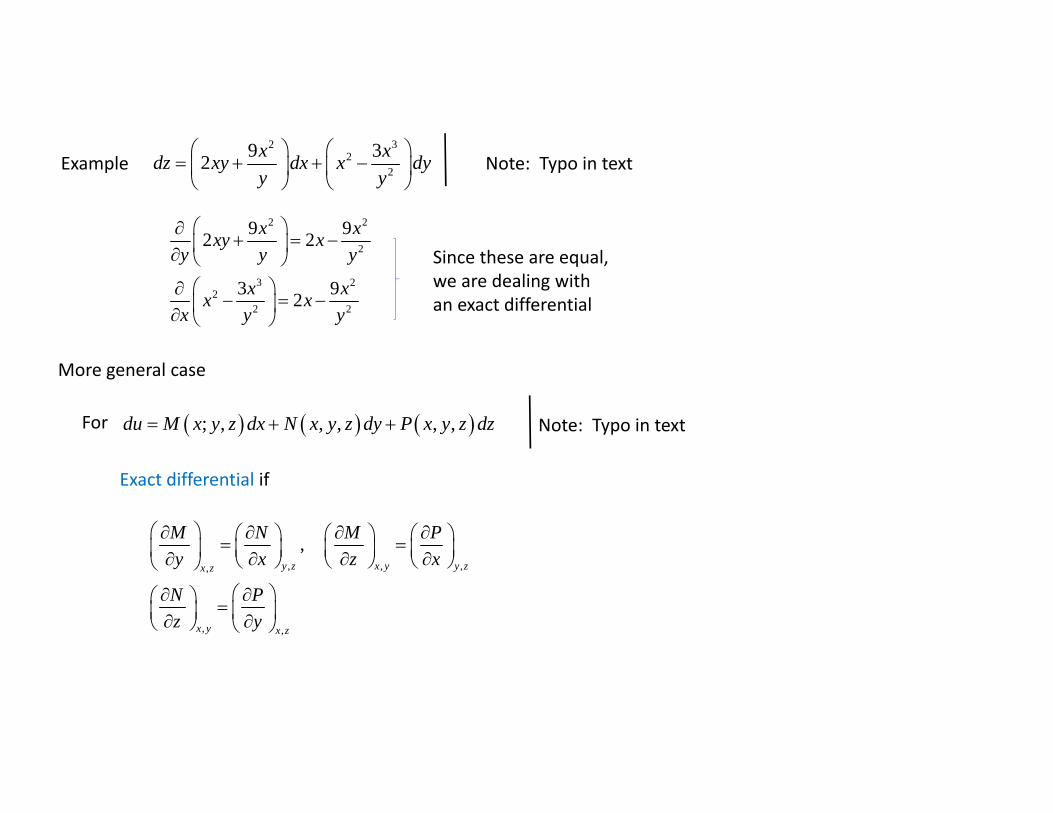
Example2 3

22

9 32 x xdz xy dx x dyy y

Note:  Typo in text

2 2

2

3 22

2 2

9 92 2

3 92

x xxy xy y y

x xx xx y y

Since these are equal,we are dealing withan exact differential

For  ; , , , , ,du M x y z dx N x y z dy P x y z dz Note:  Typo in text

Exact differential if

, , ,,

, ,

, y z x y y zx z

x y x z

M N M Py x z x

N Pz y

More general case

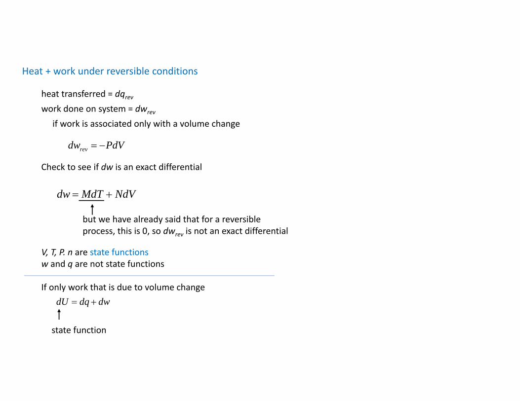
Heat + work under reversible conditions

heat transferred = dqrevwork done on system = dwrev

if work is associated only with a volume change

revdw PdV

Check to see if dw is an exact differential

dw MdT NdV

but we have already said that for a reversibleprocess, this is 0, so dwrev is not an exact differential

V, T, P. n are state functionsw and q are not state functions

If only work that is due to volume changedU dq dw

state function

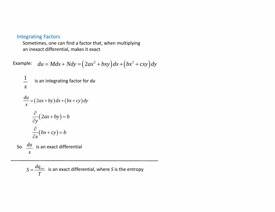
Integrating FactorsSometimes, one can find a factor that, when multiplyingan inexact differential, makes it exact

Example: 2 22du Mdx Ndy ax bxy dx bx cxy dy

1x

is an integrating factor for du

2du ax by dx bx cy dyx

2ax by by

bx cy bx

So            is an exact differentialdux

is an exact differential, where S is the entropy revdqST

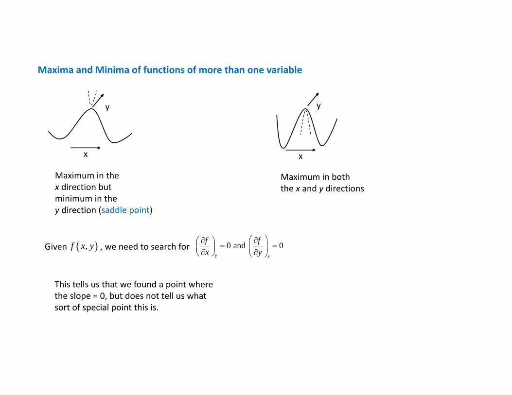
Maxima and Minima of functions of more than one variable

y

x x

y

Maximum in the x direction butminimum in they direction (saddle point)

Maximum in boththe x and y directions

Given               , we need to search for ,f x y 0 and 0y x

f fx y

This tells us that we found a point wherethe slope = 0, but does not tell us whatsort of special point this is.

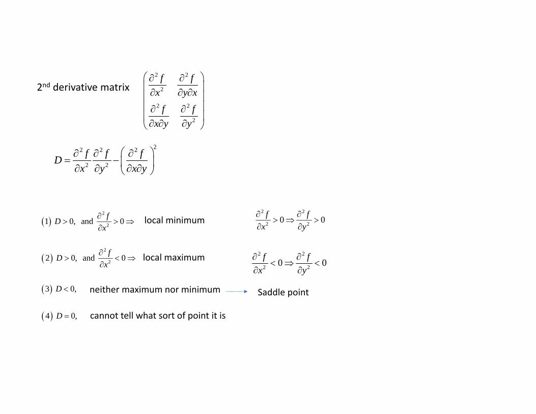
2nd derivative matrix2 2

2

2 2

2

f fx y x

f fx y y

22 2 2

2 2

f f fDx y x y

local minimum

local maximum

neither maximum nor minimum

cannot tell what sort of point it is

2

2

2

2

1 0, and 0

2 0, and 0

3 0,

4 0,

fDx

fDx

D

D

2 2

2 2 0 0f fx y

2 2

2 2 0 0f fx y

Saddle point

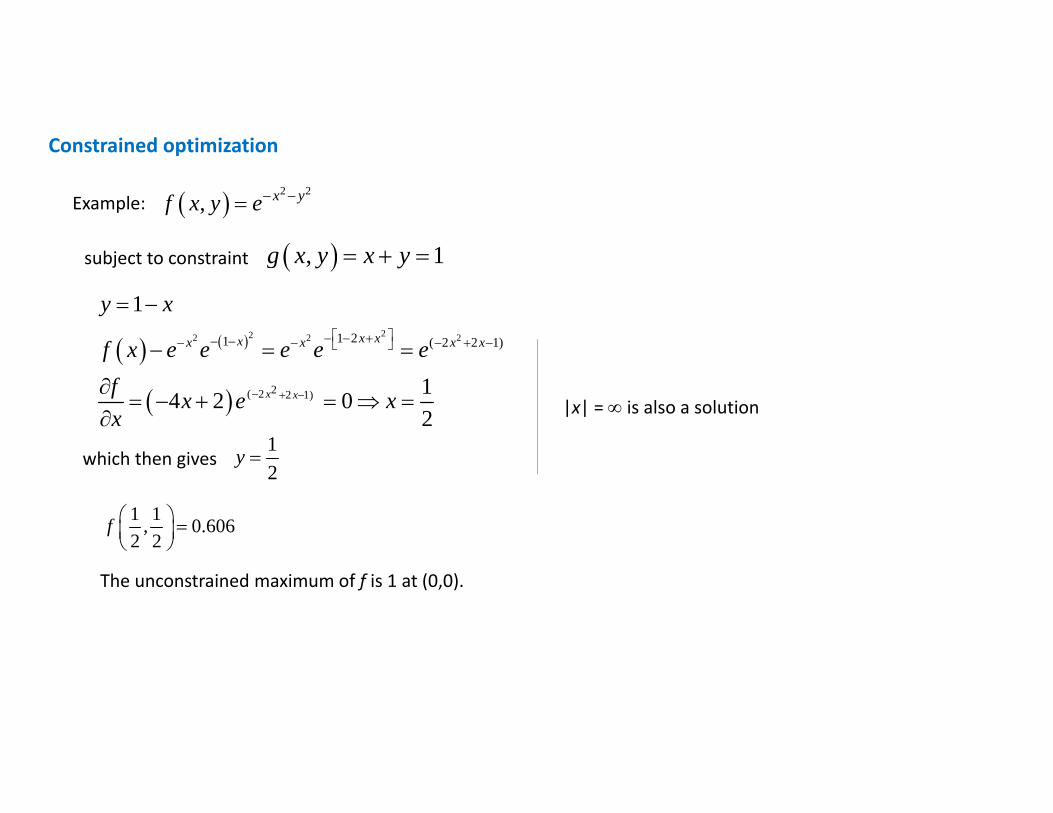
Constrained optimization

Example: 2 2, x yf x y e

subject to constraint  , 1g x y x y

222 2 2

2( 2 2 1)

1 21 ( 2 2 1)

1

14 2 02

x x

x xxx x x x

y x

f x e e e e ef x e xx

|x| =  is also a solution

1 1, 0.6062 2

f

The unconstrained maximum of f is 1 at (0,0).

which then gives 12

y

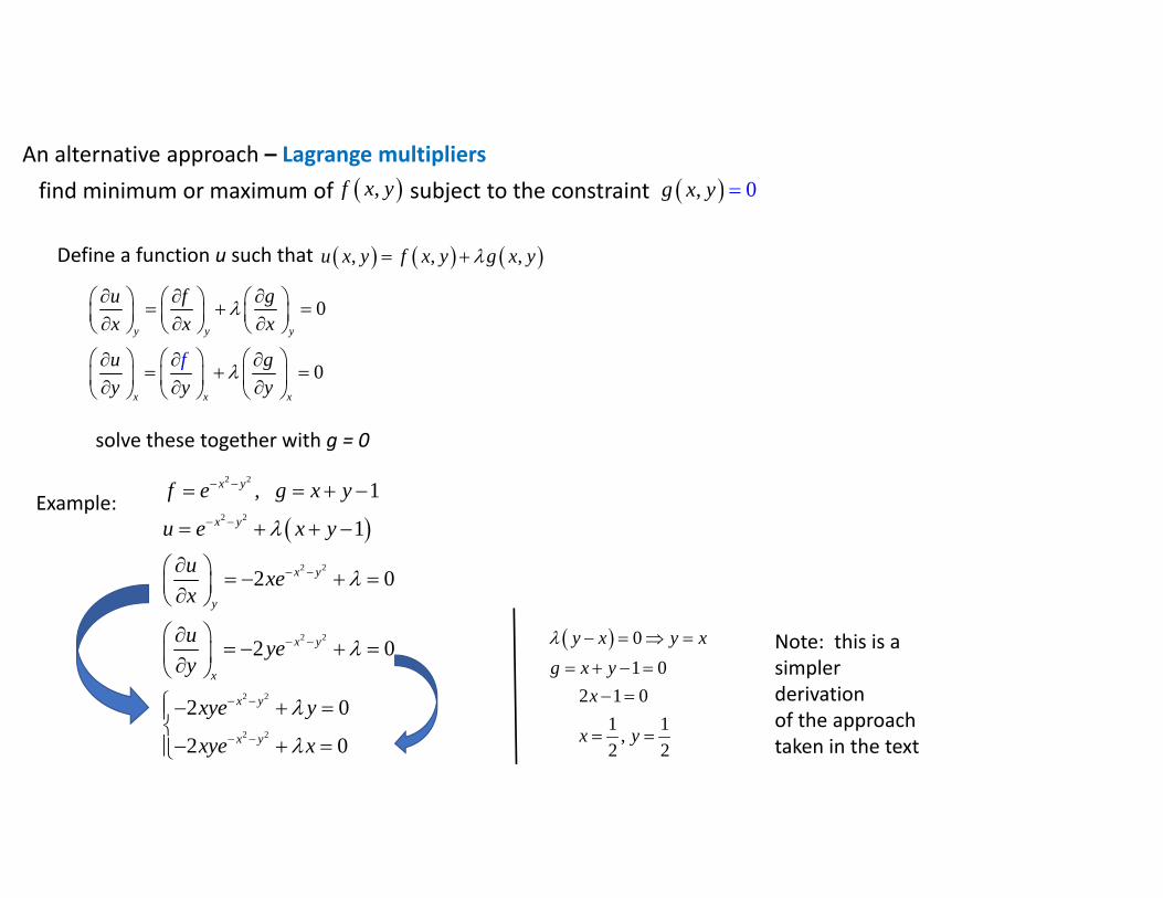
An alternative approach – Lagrange multipliersfind minimum or maximum of              subject to the constraint  ,f x y , 0g x y

Define a function u such that , , ,u x y f x y g x y

0

0

y y y

x x x

f

u f gx x x

u gy y y

solve these together with g = 0

Example:

2 2

2 2

2 2

2 2

2 2

2 2

, 1

1

2 0

2 0

2 0

2 0

x y

x y

x y

y

x y

x

x y

x y

f e g x y

u e x y

u xex

u yey

xye y

xye x

Note:  this is a simpler derivationof the approach taken in the text

01 0

2 1 01 1,2 2

y x y xg x y

x

x y

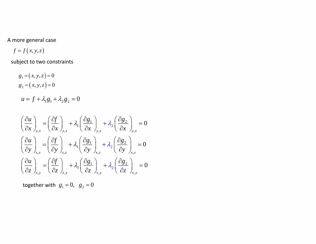
A more general case

, ,f f x y z

subject to two constraints

1

2

, , 0

, , 0

g x y z

g x y z

2

2

1 1 2 2

1 21

, , , ,

1 21

, , , ,

1 21

, , ,2

0

0

0

y z y z y z y z

x z x z x z x z

x y x y x y x

u f g g

g gu fx x x x

g gu fy y y y

gu fz z z

gz

,

0y

together with  1 20, 0g g

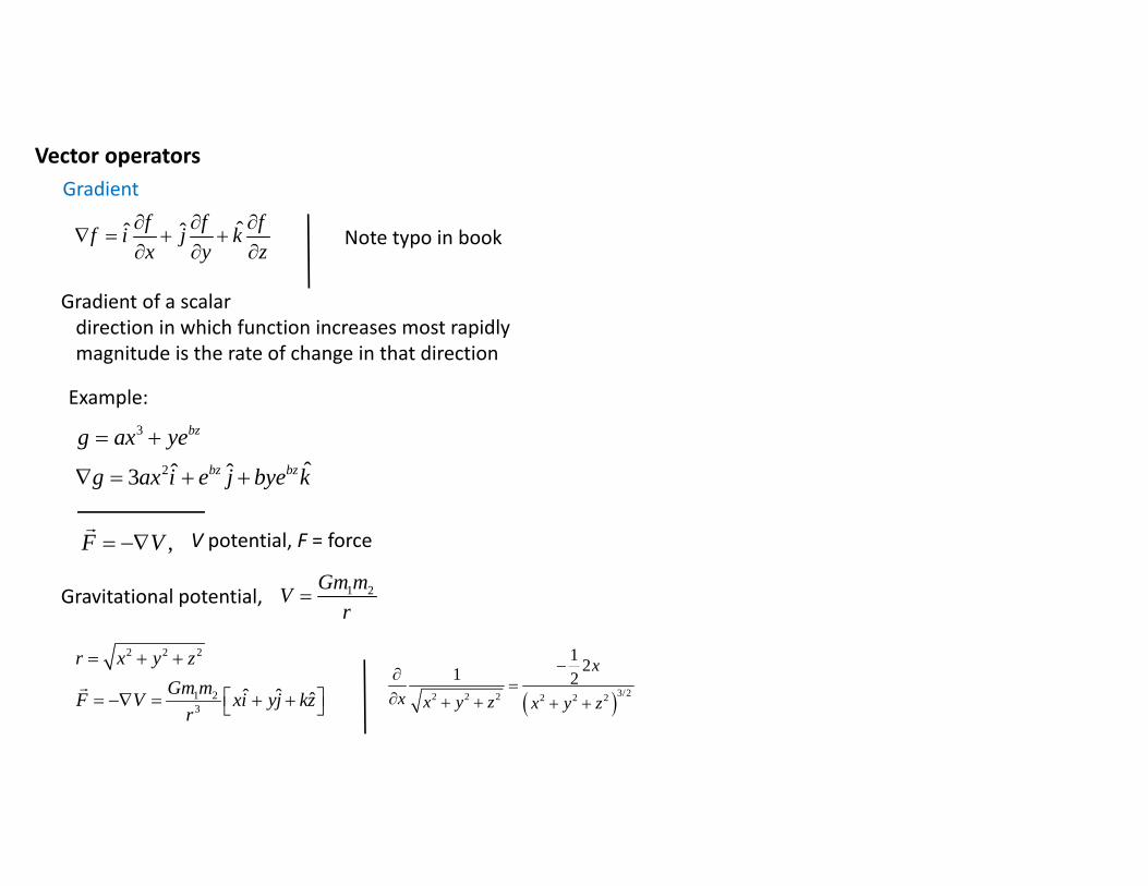
Vector operatorsGradient

ˆˆ ˆf f ff i j kx y z

Note typo in book

Gradient of a scalardirection in which function increases most rapidlymagnitude is the rate of change in that direction

Example:3

2 ˆˆ ˆ3

bz

bz bz

g ax ye

g ax i e j bye k

,F V

V potential, F = force

Gravitational potential,  1 2Gm mVr

2 2 2

1 23

ˆ ˆ ˆ

r x y zGm mF V xi yj kz

r

3/22 2 2 2 2 2

1 21 2x

x x y z x y z

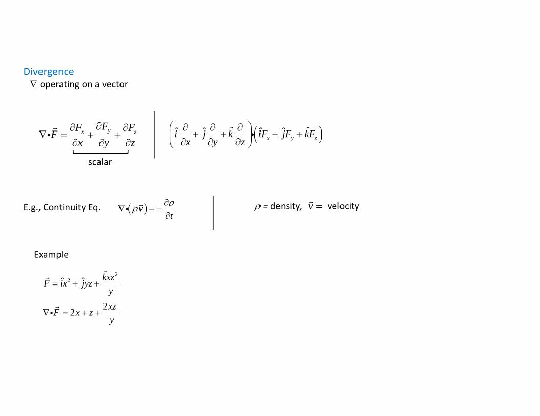
Divergence operating on a vector

yx zFF FF

x y z

scalar

ˆ ˆˆ ˆ ˆ ˆx y zi j k iF jF kF

x y z

E.g., Continuity Eq. vt

= density,           velocity

Example

22

ˆˆ ˆ

22

kxzF ix jyzyxzF x zy

v

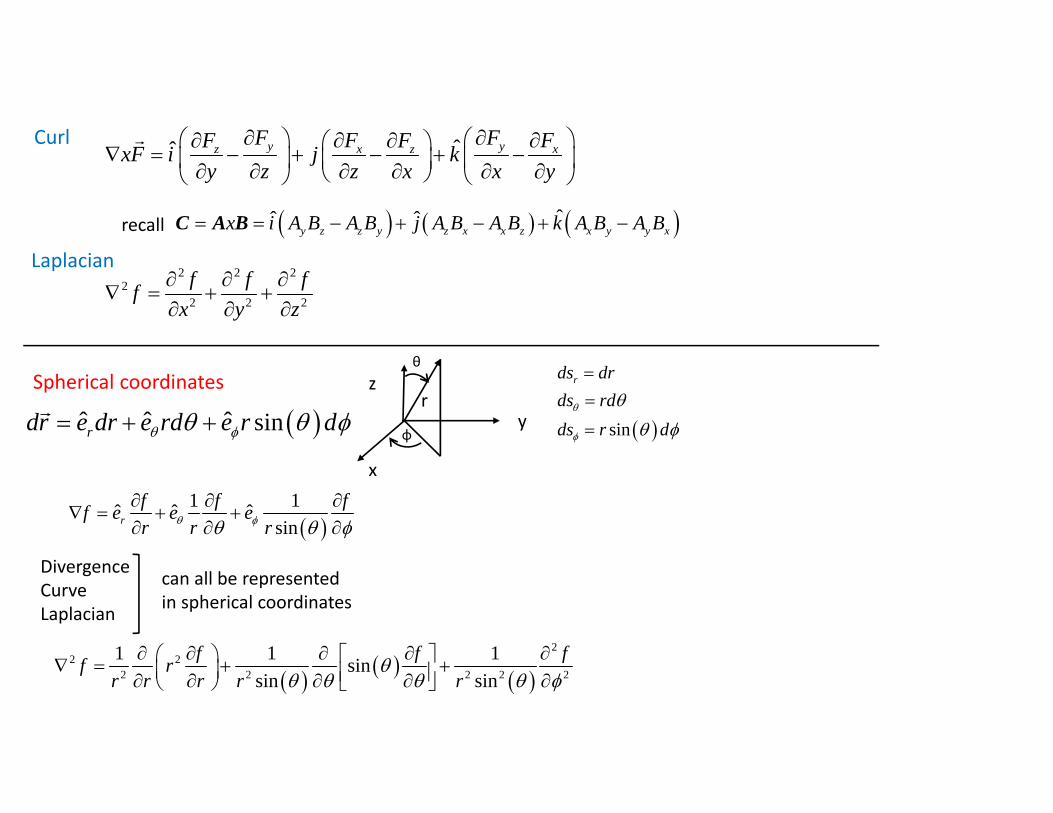
Curl ˆˆ y yx xz zF FF FF FxF i j k

y z z x x y

recall ˆˆ ˆy z z y z x x z x y y xx i A B A B j A B A B k A B A B C A B

Laplacian2 2 2

22 2 2

f f ffx y z

Spherical coordinates z

x

y

θ

φ

r sin

rds drds rdds r d

1 1ˆ ˆ ˆ

sinrf f ff e e er r r

ˆ ˆ ˆ sinrdr e dr e rd e r d

DivergenceCurveLaplacian

can all be representedin spherical coordinates

2

2 22 2 2 2 2

1 1 1sinsin sin

f f ff rr r r r r