Embed Size (px)
Citation preview

HAL Id: hal-03319784https://hal.archives-ouvertes.fr/hal-03319784
Submitted on 13 Aug 2021
HAL is a multi-disciplinary open accessarchive for the deposit and dissemination of sci-entific research documents, whether they are pub-lished or not. The documents may come fromteaching and research institutions in France orabroad, or from public or private research centers.
L’archive ouverte pluridisciplinaire HAL, estdestinée au dépôt et à la diffusion de documentsscientifiques de niveau recherche, publiés ou non,émanant des établissements d’enseignement et derecherche français ou étrangers, des laboratoirespublics ou privés.
Multistability of saxophone oscillation regimes and itsinfluence on sound production
Tom Colinot, Christophe Vergez, Philippe Guillemain, Jean-Baptiste Doc
To cite this version:Tom Colinot, Christophe Vergez, Philippe Guillemain, Jean-Baptiste Doc. Multistability of saxophoneoscillation regimes and its influence on sound production. Acta Acustica, Les Ulis, France : LesEditions de Physique, 2021, 5, pp.33. �10.1051/aacus/2021026�. �hal-03319784�

Multistability of saxophone oscillation regimes and its influence on
sound production
Tom Colinota, Christophe Vergeza, Philippe Guillemaina, Jean-Baptiste Docba Aix Marseille Univ, CNRS, Centrale Marseille, LMA, Marseille, France
b Laboratoire de Mecanique des Structures et des Systemes couples, Conservatoire Nationaldes Arts et Metiers, Paris, France
Summary1
The lowest fingerings of the saxophone can lead to2
several different regimes, depending on the musician’s3
control and the characteristics of the instrument. This4
is explored in this paper through a physical model5
of saxophone. The Harmonic Balance Method shows6
that for many combinations of musician control pa-7
rameters, several regimes are stable. Time-domain8
synthesis is used to show how different regimes can9
be selected through initial conditions and the initial10
evolution (rising time) of the blowing pressure, which11
is explained by studying the attraction basin of each12
stable regime. These considerations are then applied13
to study how the produced regimes are affected by14
properties of the resonator. The inharmonicity be-15
tween the first two resonances is varied in order to find16
the value leading to the best suppression of unwanted17
overblowing. Overlooking multistability in this de-18
scription can lead to biased conclusions. Results for19
all the lowest fingerings show that a slightly positive20
inharmonicity, close to that measured on a saxophone,21
leads to first register oscillations for the greatest range22
of control parameters. A perfect harmonicity (inte-23
ger ratio between the first two resonances) decreases24
first register production, which adds nuance to one25
of Benade’s guidelines for understanding sound pro-26
duction . Thus, this study provides some a posteriori27
insight into empirical design choices relative to the28
saxophone.29
1 Introduction30
A classic endeavor in musical acoustics consists in31
the systematic study of sound production features32
of a musical instrument. Early studies use an arti-33
ficial mouth to replace the musician (on the clarinet34
[45, 1, 60, 20] or the bassoon [28]) in order to bet-35
ter describe and understand the physical phenomena36
at play during sound production. Later on, artificial37
mouths have been robotized to provide a complete38
mapping of the instrument’s behavior, aiming at un-39
derstanding how the instrument must be acted on to40
produce different sounds [34, 42] or describing the41
influence of an acoustical parameter of the resonator 42
on sound production [23]. The objective of this last 43
study is shared by other works using a rather differ- 44
ent approach to systematic description of the instru- 45
ment’s behavior: using a physical model. Based on 46
oscillation thresholds for instance[27], some conclu- 47
sions can be drawn as to the acoustical characteristics 48
facilitating the production of sound. Numerical res- 49
olution of the model’s equations also constitute a re- 50
peatable way to map the produced sound to the char- 51
acteristics of the instruments, which has direct appli- 52
cations in instrument making [58, 25]. However, from 53
a mathematical perspective, as nonlinear dynamical 54
systems, wind instruments models often admit multi- 55
ple solutions for a given set of parameters. The ques- 56
tion of the stability of each of these solutions holds 57
great importance when aiming to describe or predict 58
the playability of an instrument based on its physical 59
model. But some important questions remain unan- 60
swered, even for ideal cases where the stability or in- 61
stability of each regime would be known. For instance, 62
which regime is produced if two regimes are stable for 63
the same control parameters combination? 64
In the case of such coexistence of stable solutions, 65
denominated multistability hereafter, the convergence 66
towards one or the other solution depends on the ini- 67
tial conditions. Indeed, each solution is associated 68
with a region of attraction or attraction basin, defined 69
as the region of the phase space where all initial con- 70
ditions converge towards this solution [52, 50]. For in- 71
stance, attraction basins are studied in walking mod- 72
els [51, 43], where the ‘walking’ (periodic) regime al- 73
most always coexists with a stable equilibrium, corre- 74
sponding to falling. In this case, describing attraction 75
basins informs control strategies in robotics [61, 62]. 76
Attraction basins are also studied for classic dynami- 77
cal oscillators, such as Chua’s circuit [44], with exper- 78
imental explorations of the attraction basins [48] as 79
well as numerical investigations [55]. As strongly non- 80
linear self-oscillating systems capable of multiple os- 81
cillating regimes, wind instrument models are among 82
the systems for which studying attraction basins can 83
shed light on their rich behavior and help understand 84
control strategies used by musicians. However, to our 85

Colinot et al., p. 2
knowledge, no study on the attraction basins of mu-86
sical instruments has been produced, although sev-87
eral studies explore their multistability. Experimen-88
tal work on the clarinet [37] and a numerical study of89
several idealized woodwind resonators [56] illustrate90
in particular the hysteresis between regimes, which91
is a consequence of multistability. On the flute, con-92
tinuation and synthesis have been used to investigate93
the hysteresis between regimes, notably depending on94
inharmonicity [57].95
Describing the attraction basins and comparing96
their sizes is expected to give information on which97
regime is most likely produced, assuming some prob-98
abilistic repartition of the initial conditions in the99
phase space [10]. However, an exhaustive description100
is almost impossible for a complete model of instru-101
ment, where the phase space is of very large dimen-102
sion. In such cases, attraction basins may be partially103
explored, based on a reduction of the phase space to104
one or two dimensions. For instance, the infinite-105
dimensional phase space of a delayed system can be106
partially described along two dimensions [59]. In the107
case of musical instruments, a reduction of the phase108
space is proposed in this paper, based on knowledge109
of typical musical scenarios. Throughout this work,110
the case of a model of saxophone is considered, and111
two scenarios are studied: transition from another es-112
tablished limit-cycle (scenario number 1), and first113
attack transient of a note, where the blowing pres-114
sure parameter goes from 0 to a certain final value115
(scenario number 2).116
Section 2 presents the physical saxophone model117
and the two numerical methods used to solve its118
equations: the Harmonic Balance Method and time-119
domain synthesis. Next, multistability is introduced120
by computing the bifurcation diagram with the har-121
monic balance method and continuation (Asymptotic122
Numerical Method) and exhibiting hysteresis cycles123
using time-domain synthesis in Section 3 (control sce-124
nario number 1). Then, in Section 4, a simple test-125
case of scenario number two is presented to study126
sound production, where the blowing pressure in-127
creases from 0 to its final value over different du-128
rations. We show how this duration can influence129
the final regime in multistability regions, and explain130
these results by presenting the attraction basin of each131
regime. Section 5 demonstrates how the awareness of132
multistability can lead to a better description of the133
behavior of the model. Depending on the inharmonic-134
ity of the resonator, the size of the control parame-135
ter regions where each regime appears in synthesis136
is described, taking into account multistability. This137
provides an interpretation to the inharmonicity value138
measured on the saxophone by showing that it corre-139
sponds to an optimum in periodic regime production.140
2 Numerical simulation frame- 141
work 142
2.1 Saxophone model 143
The saxophone model used in this study is comprised 144
of three main elements: a one degree-of-freedom os- 145
cillator representing the reed, a regularized nonlin- 146
ear characteristic giving the flow through the reed 147
channel, and a modal description of the measured 148
impedance of the resonator. Similar models solved 149
by time-domain synthesis (Section 2.2) are used in 150
conjunction with analytical techniques to study the 151
playing frequency [19] and spectrum [49] of clarinets, 152
as well as their radiated power with a comparison to 153
measurements [33]. The Harmonic Balance Method 154
(Section 2.3) can also be applied to this model to 155
study its dynamic behavior, for instance to quantify 156
the effect of neglecting reed contact [18]. 157
Dimensionless [28, 35] acoustical Kirchhoff vari-ables (p, u) are used in this work:
p =p
pM, u = Zc
u
pM, (1)
where the hat notation indicates the variable in phys-ical unit, pM is the static pressure necessary to closethe reed channel completely and Zc is the characteris-tic input impedance of the resonator for plane waves.Similarly, the reed displacement from equilibrium isgiven in dimensionless form
x =x
H(2)
where H is the distance between the reed and themouthpiece lay at rest. With this formalism, the reedchannel is closed when x ≤ −1. In this work, the onlytime-varying control parameter [60] is the dimension-less blowing pressure γ:
γ(t) =pm(t)
pM, (3)
where pm is the physical value of the pressure in the 158
mouth of the musician. We leave all other control pa- 159
rameters constant in order to limit the dimensionality 160
of the study. The values and names of the parameters 161
are summarized in Table 1 and detailed below through 162
the model description. Their values are drawn from 163
[46] for the reed parameters qr and ωr, from [13] for 164
the order of magnitude of the contact stiffness Kc. 165
2.1.1 The reed model 166
Following [13], the reed is modeled by a single de-gree of freedom oscillator including a nonlinear con-tact force accounting for the mouthpiece lay
x
ω2r
+qrωrx+ x = p− γ + Fc(x+ 1), (4)

Colinot et al., p. 3
Name Symbol Value
Blowing pressure γ VariableReed opening at rest ζ 0.6
Reed damping qr 1Reed eigenfrequency ωr 4224 rad.s−1
Mouthpiece lay stiffness Kc 100
Contact regularization η 10−3
Number of modes Nm 8Number of harmonics H 20
Table 1: Parameters of the numerical model: musi-cian control parameters γ and ζ, reed parameters qrand ωr, contact parameter Kc and parameters inher-ent to the numerical implementation η, Nm and H.
where the two parameters of the reed are its angulareigenfrequency ωr and its damping coefficient qr, andthe contact force is a function of the dimensionlessreed opening x+ 1 and is taken from [8],
Fc(x+ 1) = Kcmin(x+ 1, 0)2, (5)
where Kc = 100. Since x+ 1 is the distance betweenthe reed and the mouthpiece lay, Fc can be interpretedas a quadratic stiffness activated whenever the reedtouches the lay. The ramp function min(x + 1, 0) isregularized using a parameter η = 10−3 to avoid non-differentiability at x = −1 (reed closure)
min(x+ 1, 0) 'x+ 1−
√(x+ 1)2 + η
2. (6)
The regularization controlled by parameter η is nec-167
essary for the system to fit the quadratic formalism168
required by the implementation of the harmonic bal-169
ance method and asymptotic numerical continuation170
in the MANLAB software, which produces the bifur-171
cation diagrams of the present article. Although the172
parameter η is not necessary for the time-domain syn-173
thesis method to function, it is kept for comparison174
purposes.175
2.1.2 The reed channel176
The flow at the input of the resonator is deduced fromBernoulli’s law [2, 36] applied to the reed channel andturbulent mixing into the mouthpiece
u = ζmax(x+ 1, 0)sign(γ − p)√|γ − p| (7)
where ζ is the dimensionless control parameter ac-counting for reed opening at rest
ζ = ZcwH
√2
ρ, (8)
w being the effective width of the reed channel and ρthe density of the medium. We choose to ignore theflow due to the speed of the reed [19, 21] in the present
model, as it only has a small effect on the playingfrequency, which is not discussed here. The absolutevalue and ramp function in Eq. (7) are regularizedwith the same parameter η as in Eq. (6)
|γ − p| '√
(γ − p)2 + η, (9)
max(x+ 1, 0) 'x+ 1 +
√(x+ 1)2 + η
2. (10)
2.1.3 The resonator 177
The input impedance is used to represent the res-onator’s acoustical response. The dimensionless in-put impedance Z(ω) of a Buffet-Crampon Senzo altosaxophone is measured with the CTTM impedancesensor [22]. The saxophone is measured withoutits mouthpiece, placing the reference plane of theimpedance measurement at the input cross-section ofthe crook. A cylindrical tube is added by TransferMatrix Method [12] in post-processing to representthe mouthpiece, before using it in synthesis. Thelength of the cylinder is 60 mm and the radius is thesame as the input radius of the crook, 6 mm. Thetotal volume of the added cylinder approximately fitsthat of the missing cone apex, as per a classical aca-demic approximation [38]. In order to use this inputimpedance for the two numerical synthesis methodspresented above, it is decomposed into modes [19] sothat
Z(ω) =
Nm∑n=1
Cnjω − sn
+C∗n
jω − s∗n, (11)
where Cn and sn are the estimated complex modalresidues and poles [54] andNm is the number of modesretained in the simulation. In this paper Nm = 8modes are used. This translates into the time do-main by describing the pressure as a sum of complexmodal components pn, whose evolution depends onthe modal coefficients, such that
pn(t)− snpn(t) = Cnu(t), ∀n ∈ [1, Nm], (12)
p(t) = 2
Nm∑n=1
Re(pn(t)). (13)
The flow u in (12) is given by (7). Figure 1 displays 178
the measured impedance and the associated modal 179
reconstruction according to Eq. (11) for the D] fin- 180
gering used throughout the rest of this article. The 181
corresponding modal coefficients Cn and poles sn are 182
summarized in Table 2. Note that the choice of 183
a modal formalism over a direct resolution of partial 184
differential equations in the resonator is made here be- 185
cause of its lower computational cost and number of 186
variables, which facilitates large-scale numerical stud- 187
ies such as those presented in Section 5. Addition- 188
ally, the modal formalism involves a limited number 189
of parameters, which are directly tied to the acoustics 190

Colinot et al., p. 4
Residues Cn (unitless) Poles sn (rad.s−1)176.1 −17.59 + j1195470.5 −35.50 + j2483649.4 −65.30 + j3727328.7 −269.34 + j4405541.5 −70.32 + j5153224.9 −166.0 + j6177382.2 −94.49 + j6749409.9 −116.5 + j7987
Table 2: Modal parameters for the fingering D] of thealto saxophone.
of the resonator, instead of the complete geometri-191
cal description that a wave propagation model would192
require.193
Figure 1: Measured input impedance (solid) andmodal reconstruction (dashed) for the fingering D]of the alto saxophone.
2.2 Time-domain synthesis194
Equations (4), (7) and (12) are discretized using195
finite-difference approximations for the time-domain196
derivatives, following a discretization scheme first ap-197
plied to simple waveguides [29] and then adapted to198
a modal formalism [19]. The reader can find a de-199
tailed description of this discretization scheme in a200
recent document [16]. The sampling rate used in the201
simulation is Fs = 176400 Hz, four times higher than202
the standard audio sampling rate. Such a high sam-203
pling rate is required, given the chosen finite differ-204
ence scheme, to give precise results that match those205
obtained with the harmonic balance method.206
As an illustrative result, Figure 2 shows an exam-207
ple of the synthesized pressure signal and its spectro-208
gram. Note that the signal shown is a portion of the209
signal used in Figure 4, with control scenario num- 210
ber one. It corresponds to the first occurrence of 211
the oscillations at a blowing pressure value γ ' 0.45. 212
At this point, the system jumps from equilibrium to 213
the first register and passes through fleeting second 214
register and quasi periodic regimes. The spectrogram 215
(Figure 2 (b)) shows the second register to be the oc- 216
tave (double the fundamental frequency) of the first 217
register. The quasi-periodic portion of the signal dis- 218
plays amplitude variations, seen in the envelope of the 219
signal (Figure 2 (a)) and on the odd harmonic com- 220
ponents of the spectrogram. Quasi-periodic regimes 221
are well-known on saxophone-like instrument models, 222
documented for instance in [20, 24, 23]. 223
(a)
-60
-50
-40
-30
-20
-10
0
(b)
Figure 2: Time-domain synthesized pressure signal.(a) temporal envelope (black) and blowing pressureparameter γ (red). (b) Normalized spectrogram(dB) with regime names indicated (unstable ones be-tween parentheses) : equilibrium (Eq.), second reg-ister, quasi-periodic and first register. The signal isextracted from the same blowing pressure ramp as inFigure 4, between γ = 0.45 and γ = 0.51 (at first oc-currence of oscillation).
Colinot et al., p. 5
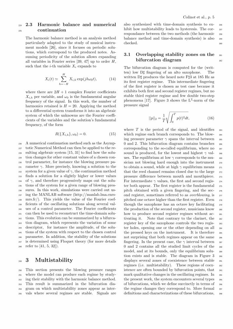
2.3 Harmonic balance and numerical224
continuation225
The harmonic balance method is an analysis methodparticularly adapted to the study of musical instru-ment models [26], since it focuses on periodic solu-tions, which correspond to the produced notes. As-suming periodicity of the solution allows expandingall variables in Fourier series [39, 47] up to order H,such that the i-th variable Xi expands to
Xi(t) 'H∑
h=−H
Xi,h exp(jhω0t), (14)
where there are 2H + 1 complex Fourier coefficientsXi,h per variable, and ω0 is the fundamental angularfrequency of the signal. In this work, the number ofharmonics retained is H = 20. Applying the methodto a differential system transforms it into an algebraicsystem of which the unknowns are the Fourier coeffi-cients of the variables and the solution’s fundamentalfrequency, of the form
R({Xi,h}, ω0) = 0. (15)
A numerical continuation method such as the Asymp-226
totic Numerical Method can then be applied to the re-227
sulting algebraic system [15, 31] to find how the solu-228
tion changes for other constant values of a chosen con-229
trol parameter, for instance the blowing pressure pa-230
rameter γ. More precisely, knowing a solution to the231
system for a given value of γ, the continuation method232
finds a solution for a slightly higher or lower values233
of γ, and therefore progressively maps out the solu-234
tions of the system for a given range of blowing pres-235
sures. In this work, simulations were carried out us-236
ing the MANLAB software (http://manlab.lma.cnrs-237
mrs.fr/). This yields the value of the Fourier coef-238
ficients of the oscillating solutions along several val-239
ues of a control parameter. The Fourier coefficients240
can then be used to reconstruct the time-domain solu-241
tions. This evolution can be summarized by a bifurca-242
tion diagram, which represents the variation of some243
descriptor, for instance the amplitude, of the solu-244
tions of the system with respect to the chosen control245
parameter. In addition, the stability of the solutions246
is determined using Floquet theory (for more details247
refer to [41, 5, 32]).248
3 Multistability249
This section presents the blowing pressure ranges250
where the model can produce each regime by study-251
ing their stability with the harmonic balance method.252
This result is summarized in the bifurcation dia-253
gram on which multistability zones appear as inter-254
vals where several regimes are stable. Signals are255
also synthesized with time-domain synthesis to ex- 256
hibit how multistability leads to hysteresis. The cor- 257
respondance between the two methods (the harmonic 258
balance method and time-domain synthesis) is also 259
checked. 260
3.1 Overlapping stability zones on the 261
bifurcation diagram 262
The bifurcation diagram is computed for the (writ-ten) low D] fingering of an alto saxophone. Thewritten D] produces the heard note F]3 at 185 Hz asits first register regime. This intermediate fingeringof the first register is chosen as test case because itexhibits both first and second register regimes, but nostable third register regime and few double two-stepphenomena [17]. Figure 3 shows the L2-norm of thepressure signal
||p||2 =1
T
√∫ T
0
p(t)2dt, (16)
where T is the period of the signal, and identifies 263
which regime each branch corresponds to. The blow- 264
ing pressure parameter γ spans the interval between 265
0 and 2. This bifurcation diagram contains branches 266
corresponding to the so-called equilibrium, where no 267
sound is produced, for the lowest and highest γ val- 268
ues. The equilibrium at low γ corresponds to the mu- 269
sician not blowing hard enough into the instrument 270
to obtain a sound, while at high γ equilibrium means 271
that the reed channel remains closed due to the large 272
pressure difference between mouth and mouthpiece. 273
For intermediate γ values, the first and second regis- 274
ter both appear. The first register is the fundamental 275
pitch obtained with a given fingering, and the sec- 276
ond register, sometimes referred to as overblowing, is 277
pitched one octave higher than the first register. Even 278
though the saxophone has an octave key facilitating 279
the production of the second register, musicians know 280
how to produce second register regimes without ac- 281
tivating it. Note that contrary to the clarinet, the 282
register key of the saxophone controls the two regis- 283
ter holes, opening one or the other depending on all 284
the pressed keys on the instrument. It is therefore 285
not surprising that both regimes appear on the same 286
fingering. In the present case, the γ interval between 287
0 and 2 contains all the studied limit cycles of the 288
model, and at its bounds, only the equilibrium solu- 289
tion exists and is stable. The diagram in Figure 3 290
displays several zones of coexistence between stable 291
regimes (i.e. multistability). These regions of coex- 292
istence are often bounded by bifurcation points, that 293
mark qualitative changes in the oscillating regimes. In 294
the present work, the system encounters several types 295
of bifurcations, which we define succinctly in terms of 296
the regime changes they correspond to. More formal 297
definitions and characterizations of these bifurcations, 298

Colinot et al., p. 6
notably in terms of critical values of the eigenvalues299
of the jacobian matrix of the system, can be found300
in [40, 7]. The Hopf bifurcation marks the emergence301
of an oscillating solution from equilibrium. The fold302
bifurcation corresponds to a stable and unstable solu-303
tion branch colliding and disappearing, which can be304
better seen on the bifurcation diagrams as limit points305
in the solution branches. Neimark-Sacker bifurcations306
correspond to a periodic regime becoming unstable307
and being replaced by a quasi-periodic regime. A de-308
generate case of the Neimark-Sacker bifurcations is309
the period-doubling bifurcation, where a periodic so-310
lution of halved frequency emerges from an oscillating311
solution. On saxophone models, period doubling bi-312
furcations transform a second register regime into a313
first register. As is discussed in the next paragraph314
for the saxophone, Hopf and fold bifurcations often315
delimit coexistence between the equilibrium and an316
oscillating regime, while Neimark-Sacker and period-317
doubling bifurcations mark the limits of multistability318
regions between two oscillating regimes.319
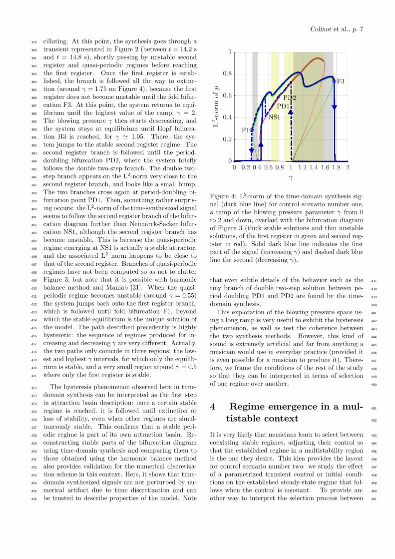
Figure 3: Bifurcation diagram obtained with har-monic balance method and numerical continuation:L2-norm of the acoustical pressure depending on theblowing pressure parameter γ for the low written D]fingering of an alto saxophone. Thick lines: stablesolution, thin lines: unstable solutions. Black: equi-librium, green: 1st register regimes, red: 2nd registerregimes. Multistability zones are shaded: light yel-low where 1st and 2nd register coexist, darker grayfor equilibrium and 1st register. Blue circles specifythe location of bifurcations. Vertical black lines corre-spond to those in Figure 6 (c), and (from left to right)to phase diagrams 7 (a), (b) and (c).
Starting from low blowing pressure values, the first320
coexistence zone appears between the first register321
and the equilibrium. It is delimited by the fold bi-322
furcation F1 of the first register around γ = 0.3 and 323
the inverse Hopf bifurcation H1 at γ = 0.4 where 324
the equilibrium becomes unstable. The second coexis- 325
tence zone is between first and second register, in the 326
interval where the second register is stable between 327
the Neimark-Sacker bifurcation NS1 and the period- 328
doubling bifurcation PD1 (respectively at γ = 0.66 329
and γ = 0.79). The Neimark-Sacker bifurcation NS1 330
mark the destabilization of the second register and 331
the emergence of a quasi-periodic regime (not repre- 332
sented here), sometimes called multiphonics by musi- 333
cians. The next coexistence zone occurs in the in- 334
terval between the two period-doubling bifurcations 335
PD1 and PD2 on the second register branch, where a 336
stable double two-step solution [17] emerges. This co- 337
existence zone is not shaded on the figure, as it could 338
represent less of a musical issue, since double two-step 339
regimes have roughly the same frequency as standard 340
first register regimes. The fourth coexistence zone is 341
more complicated: it starts between first and second 342
register at the period-doubling bifurcation PD2, and 343
then the equilibrium also becomes stable at the Hopf 344
bifurcation H4. The limit of the last coexistence zone 345
is made by the two fold bifurcations F2 and F3 where 346
the first and second register solutions cease to exist. 347
The diagram in Figure 3 shows that coexistence 348
zones between stable regimes span most of the range 349
in γ where oscillating solutions exist, including ar- 350
guably crucial γ values like the lowest for which an 351
oscillating regime exists. Multistability is not an iso- 352
lated phenomenon, but rather corresponds to the gen- 353
eral situation, at least for this fingering. 354
3.2 Time-domain synthesis with blow- 355
ing pressure ramps (control sce- 356
nario number one) 357
Once multistability zones are identified, time-domain 358
synthesis can be used to exhibit their role when play- 359
ing the instrument. One of the main phenomena mul- 360
tistability entails is hysteresis: for several values of the 361
blowing pressure, a different regime is produced de- 362
pending on whether the blowing pressure is increasing 363
or decreasing. Various multistable regimes are exhib- 364
ited using this method in [56] on woodwind models. 365
Figure 4 shows the hysteresis cycles obtained by using 366
ramps of γ: in control scenario number one, the pa- 367
rameter γ is progressively increased from 0 to 2 and 368
then decreased back to 0. Each one of the increasing 369
and decreasing phases of the synthesis has a duration 370
of 60 s. This duration was chosen after several trials, 371
sufficiently long to let stable regimes establish while 372
keeping a γ slope steep enough to limit dynamical 373
bifurcation delays [6]. 374
Figure 4 shows that the synthesized signal starts 375
from γ = 0 at equilibrium, its L2-norm being zero. 376
Then, at Hopf bifurcation H1, the equilibrium be- 377
comes unstable, which causes the system to start os- 378
Colinot et al., p. 7
cillating. At this point, the synthesis goes through a379
transient represented in Figure 2 (between t = 14.2 s380
and t = 14.8 s), shortly passing by unstable second381
register and quasi-periodic regimes before reaching382
the first register. Once the first register is estab-383
lished, the branch is followed all the way to extinc-384
tion (around γ = 1.75 on Figure 4), because the first385
register does not become unstable until the fold bifur-386
cation F3. At this point, the system returns to equi-387
librium until the highest value of the ramp, γ = 2.388
The blowing pressure γ then starts descreasing, and389
the system stays at equilibrium until Hopf bifurca-390
tion H3 is reached, for γ ' 1.05. There, the sys-391
tem jumps to the stable second register regime. The392
second register branch is followed until the period-393
doubling bifurcation PD2, where the system briefly394
follows the double two-step branch. The double two-395
step branch appears on the L2-norm very close to the396
second register branch, and looks like a small bump.397
The two branches cross again at period-doubling bi-398
furcation point PD1. Then, something rather surpris-399
ing occurs: the L2-norm of the time-synthesized signal400
seems to follow the second register branch of the bifur-401
cation diagram further than Neimarck-Sacker bifur-402
cation NS1, although the second register branch has403
become unstable. This is because the quasi-periodic404
regime emerging at NS1 is actually a stable attractor,405
and the associated L2 norm happens to be close to406
that of the second register. Branches of quasi-periodic407
regimes have not been computed so as not to clutter408
Figure 3, but note that it is possible with harmonic409
balance method and Manlab [31]. When the quasi-410
periodic regime becomes unstable (around γ = 0.55)411
the system jumps back onto the first register branch,412
which is followed until fold bifurcation F1, beyond413
which the stable equilibrium is the unique solution of414
the model. The path described precedently is highly415
hysteretic: the sequence of regimes produced for in-416
creasing and decreasing γ are very different. Actually,417
the two paths only coincide in three regions: the low-418
est and highest γ intervals, for which only the equilib-419
rium is stable, and a very small region around γ = 0.5420
where only the first register is stable.421
The hysteresis phenomenon observed here in time-422
domain synthesis can be interpreted as the first step423
in attraction basin description: once a certain stable424
regime is reached, it is followed until extinction or425
loss of stability, even when other regimes are simul-426
taneously stable. This confirms that a stable peri-427
odic regime is part of its own attraction basin. Re-428
constructing stable parts of the bifurcation diagram429
using time-domain synthesis and comparing them to430
those obtained using the harmonic balance method431
also provides validation for the numerical discretiza-432
tion scheme in this context. Here, it shows that time-433
domain synthesized signals are not perturbed by nu-434
merical artifact due to time discretization and can435
be trusted to describe properties of the model. Note436
F1
F3
Figure 4: L2-norm of the time-domain synthesis sig-nal (dark blue line) for control scenario number one,a ramp of the blowing pressure parameter γ from 0to 2 and down, overlaid with the bifurcation diagramof Figure 3 (thick stable solutions and thin unstablesolutions, of the first register in green and second reg-ister in red). Solid dark blue line indicates the firstpart of the signal (increasing γ) and dashed dark blueline the second (decreasing γ).
that even subtle details of the behavior such as the 437
tiny branch of double two-step solution between pe- 438
riod doubling PD1 and PD2 are found by the time- 439
domain synthesis. 440
This exploration of the blowing pressure space us- 441
ing a long ramp is very useful to exhibit the hysteresis 442
phenomenon, as well as test the coherence between 443
the two synthesis methods. However, this kind of 444
sound is extremely artificial and far from anything a 445
musician would use in everyday practice (provided it 446
is even possible for a musician to produce it). There- 447
fore, we frame the conditions of the rest of the study 448
so that they can be interpreted in terms of selection 449
of one regime over another. 450
4 Regime emergence in a mul- 451
tistable context 452
It is very likely that musicians learn to select between 453
coexisting stable regimes, adjusting their control so 454
that the established regime in a multistability region 455
is the one they desire. This idea provides the layout 456
for control scenario number two: we study the effect 457
of a parametrized transient control or initial condi- 458
tions on the established steady-state regime that fol- 459
lows when the control is constant. To provide an- 460
other way to interpret the selection process between 461

Colinot et al., p. 8
multistable regime, a third control scenario is used,462
where only initial conditions are varied and all con-463
trol parameters are constant.464
4.1 Control scenario number two: in-465
creasing blowing pressure466
One way to study the attraction basins more thor-oughly is to run many simulations with initial con-ditions spanning the whole phase space. However,since the considered model has a 2Nm+2 dimensionalphase space, a complete exploration is not possible.Moreover, many of the possible initial conditions areunlikely to be created by the musician. More inter-esting is the exploration of the regions of the phasespace that are crossed by the system when a givencontrol pattern is varied. Here, we focus on a mono-tonic increase of the blowing pressure γ at the attack:without using the tongue, the player starts blow-ing progressively harder into the instrument. Sucha scenario was proposed in [53]. Note that instru-mented mouthpiece measurements performed on thesaxophone, such as those presented in [30], often showa different profile including a pressure overshoot be-fore the apparition of the oscillations. However, inthe present study, we omit that overshoot so that thecontrol scenario is entirely defined by a single param-eter. In control scenario number two, the blowingpressure starts from 0 and rises up until stabilizing ata certain value γf , during a certain time determinedby the parameter τg. The temporal variation of γ isgiven by the
γ(t) =γf2
(1 + tanh
(t− 5τgτg
)), (17)
which is differentiable infinitely many times. Figure467
5 displays four examples of such transients.468
Other envelopes (sigmoid, sine branch) were tested,469
only causing small quantitative changes to the results.470
Figures 6 shows which established regimes appear in471
time-domain synthesis depending on τg, for final val-472
ues γf belonging to the multistability zones described473
in Figure 3. Each dot on the figure represents the474
type of established regime after five seconds of time-475
domain synthesis. This synthesis duration was chosen476
to be sufficiently long so that the transient is com-477
pleted and the established regimes can be observed.478
Regime types are estimated using an energy-based479
criterion for equilibrium (if the energy of the pres-480
sure signals in the last ten periods is less than that of481
the first ten, the regime is classified as equilibrium)482
and a fundamental frequency estimator to determine483
the first and second register. To detect quasi-periodic484
regimes, an attribute that can be observed in Figure485
2 is used: the fact that the amplitudes of the harmon-486
ics of a quasi-periodic signal vary temporally. For the487
classification, if the mean variance of the harmonic488
Figure 5: Four examples of blowing pressure varia-tions in control scenario number two, as described by
Eq. (17), for γf = 0.4 and 0.6 and τg = τ[1]g = 10 ms
and τ[2]g = 20 ms.
amplitudes is more than a certain threshold (here set489
to 10−6), then the regime is considered quasi-periodic.490
Figure 6 (a) focuses on the first multistability re- 491
gion (highlighted in gray in Figure 3), near the first 492
Hopf bifurcation H1. The two stable regimes in this 493
region are the equilibrium ( ) and the first regis- 494
ter ( ). For final values γf between 0.38 and 0.4, 495
the system can converge to both regime depending on 496
the characteristic rising time τγ . It is interesting to 497
note that equilibrium is reached for the longest rising 498
times, i.e. the slowest γ variation, whereas the oscil- 499
lating regime is reached for the shortest rising times. 500
This is understandable as a quick γ increase tends to 501
drive the system away from equilibrium, and there- 502
fore possibly out of its attraction basin. Note that 503
some of the oscillating regimes near the limit, for the 504
longest attack times, are classified as quasi-periodic. 505
This is due to the transient being extremely long in 506
this particular region: the steady-state regime is not 507
yet established at the end of the synthesized signals. 508
This classification particularity, which could be seen 509
as an error, is not corrected because, from a musi- 510
cian’s perspective, a regime still varying five seconds 511
after the start of the attack will arguably not be con- 512
sidered periodic. 513
The second zone of multistability is explored in Fig- 514
ure 6 (b). The first and second register are separated 515
by some stable quasi-periodic regimes ( ). This is 516
the same quasi-periodic regime that appears in time- 517
domain synthesis in Figure 2, which overlays the un- 518
stable portion of the second register branch. There is 519
a particular range of characteristic time τg that seems 520
to produce the first register for a larger range of γf . 521

Colinot et al., p. 9
(a)
8 (a) 8 (b) 8 (d) 8 (e)
(b)
8 (c) 7 (a) 7 (b) 7 (c) 8 (f)
(c)
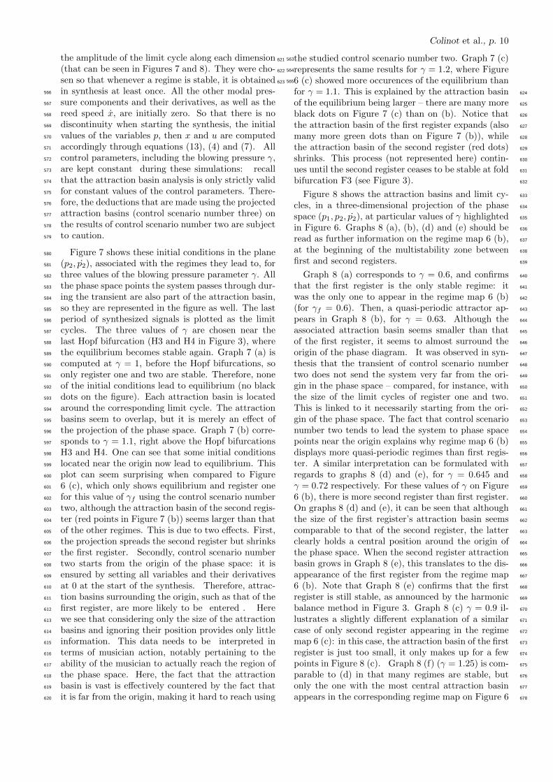
Figure 6: Classification of the steady-state regimesproduced depending on the blowing pressure transientparameters: final value γf and characteristic timeτg. Multistability zones (deduced from Figure 3): (a)equilibrium and first register (b) first register
and second register (c) all three regime types.Blue triangles indicate quasi-periodic regimes. Thehorizontal line on graph (b) shows τ = 1/f1. The ver-tical lines highlight the γ values of phase diagrams inFigure 7 and 8.
The corresponding values of τg are close to the period 522
of the first register, represented by the horizontal line 523
in 6 (b).524
In the last multistability (0.9 ≤ γ ≤ 1.25), three525
regimes may be stable for the same parameter val-526
ues, as shown on Figure 3. However, Figure 6 re-527
veals that there is no γf region where all three are528
produced. This can be explained by analyzing the529
attraction basins (see Section 4.2 Figure 8).530
4.2 Control scenario number three: 531
varying initial conditions 532
The results concerning the influence of the blowing 533
pressure parameter can be better understood by ex- 534
amining the region of the phase space leading to each 535
regime. A point in the phase space represents the 536
current state of the system, meaning the value of the 537
state variables and their derivatives. Since the sys- 538
tem is deterministic, a given point in the phase space 539
will always lead to the same stable established regime. 540
Therefore regions of the phase space can be associated 541
with each regime. These regions are called attraction 542
basins. The attraction basins are only rigorously 543
defined in a context where all control parameters are 544
constant. However, to interpret the results obtained 545
with a control parameter transient such as control sce- 546
nario number two, it is useful to observe the layout of 547
attraction basins obtained for the final blowing pres- 548
sure value γf . Specifically, at the beginning of control 549
scenario number two, the blowing pressure is subject 550
to fast variations, making a direct approach based on 551
attraction basins ill-defined. However, after the tran- 552
sient, the blowing pressure stabilizes around its final 553
value γf . To elucidate the behavior of the system 554
at this moment, subsection 4.2 performs a systemat- 555
ical analysis of its convergence with constant control 556
parameters, in which case the attraction basins rep- 557
resentations are relevant. Therefore, a third control 558
scenario is devised, where the control parameters are 559
kept strictly constant and only the initial values of 560
certain state variables of the system are modified. 561
Because the phase space is of dimension 2Nm + 2(all modal components and their derivatives, plus reedposition and speed), it is necessary to choose a pro-jection to represent the attraction basins. After sometrials, a projection of the phase space on the two firstmodal components (see Eq. (12)) and the derivativeof the second one, (p1, p2, p2), was chosen as a three-dimensional projection. These variables were chosennot only because of their physical or mathematicalmeaning, as they relate respectively to the first andsecond register, but also because they allow for theclearest visual separation of the limit cycles and at-traction basins that could be obtained by the authors.To estimate the attraction basins, time-domain syn-thesis is launched with initial conditions spanning theprojected phase space and constant control parame-ters (control scenario number three) . A total of 256initial conditions are scattered in a Latin hypercubesampling into a rectangular parallelepiped such that
pI1 ∈ [−0.2, 0.2], pI2 ∈ [−2, 2], p2I ∈ [−707, 707].
(18)
These bounds should be understood with respect to 562
Colinot et al., p. 10
the amplitude of the limit cycle along each dimension 563
(that can be seen in Figures 7 and 8). They were cho- 564
sen so that whenever a regime is stable, it is obtained 565
in synthesis at least once. All the other modal pres-566
sure components and their derivatives, as well as the567
reed speed x, are initially zero. So that there is no568
discontinuity when starting the synthesis, the initial569
values of the variables p, then x and u are computed570
accordingly through equations (13), (4) and (7). All571
control parameters, including the blowing pressure γ,572
are kept constant during these simulations: recall573
that the attraction basin analysis is only strictly valid574
for constant values of the control parameters. There-575
fore, the deductions that are made using the projected576
attraction basins (control scenario number three) on577
the results of control scenario number two are subject578
to caution.579
Figure 7 shows these initial conditions in the plane580
(p2, p2), associated with the regimes they lead to, for581
three values of the blowing pressure parameter γ. All582
the phase space points the system passes through dur-583
ing the transient are also part of the attraction basin,584
so they are represented in the figure as well. The last585
period of synthesized signals is plotted as the limit586
cycles. The three values of γ are chosen near the587
last Hopf bifurcation (H3 and H4 in Figure 3), where588
the equilibrium becomes stable again. Graph 7 (a) is589
computed at γ = 1, before the Hopf bifurcations, so590
only register one and two are stable. Therefore, none591
of the initial conditions lead to equilibrium (no black592
dots on the figure). Each attraction basin is located593
around the corresponding limit cycle. The attraction594
basins seem to overlap, but it is merely an effect of595
the projection of the phase space. Graph 7 (b) corre-596
sponds to γ = 1.1, right above the Hopf bifurcations597
H3 and H4. One can see that some initial conditions598
located near the origin now lead to equilibrium. This599
plot can seem surprising when compared to Figure600
6 (c), which only shows equilibrium and register one601
for this value of γf using the control scenario number602
two, although the attraction basin of the second regis-603
ter (red points in Figure 7 (b)) seems larger than that604
of the other regimes. This is due to two effects. First,605
the projection spreads the second register but shrinks606
the first register. Secondly, control scenario number607
two starts from the origin of the phase space: it is608
ensured by setting all variables and their derivatives609
at 0 at the start of the synthesis. Therefore, attrac-610
tion basins surrounding the origin, such as that of the611
first register, are more likely to be entered . Here612
we see that considering only the size of the attraction613
basins and ignoring their position provides only little614
information. This data needs to be interpreted in615
terms of musician action, notably pertaining to the616
ability of the musician to actually reach the region of617
the phase space. Here, the fact that the attraction618
basin is vast is effectively countered by the fact that619
it is far from the origin, making it hard to reach using620
the studied control scenario number two. Graph 7 (c)621
represents the same results for γ = 1.2, where Figure622
6 (c) showed more occurences of the equilibrium than623
for γ = 1.1. This is explained by the attraction basin 624
of the equilibrium being larger – there are many more 625
black dots on Figure 7 (c) than on (b). Notice that 626
the attraction basin of the first register expands (also 627
many more green dots than on Figure 7 (b)), while 628
the attraction basin of the second register (red dots) 629
shrinks. This process (not represented here) contin- 630
ues until the second register ceases to be stable at fold 631
bifurcation F3 (see Figure 3). 632
Figure 8 shows the attraction basins and limit cy- 633
cles, in a three-dimensional projection of the phase 634
space (p1, p2, p2), at particular values of γ highlighted 635
in Figure 6. Graphs 8 (a), (b), (d) and (e) should be 636
read as further information on the regime map 6 (b), 637
at the beginning of the multistability zone between 638
first and second registers. 639
Graph 8 (a) corresponds to γ = 0.6, and confirms 640
that the first register is the only stable regime: it 641
was the only one to appear in the regime map 6 (b) 642
(for γf = 0.6). Then, a quasi-periodic attractor ap- 643
pears in Graph 8 (b), for γ = 0.63. Although the 644
associated attraction basin seems smaller than that 645
of the first register, it seems to almost surround the 646
origin of the phase diagram. It was observed in syn- 647
thesis that the transient of control scenario number 648
two does not send the system very far from the ori- 649
gin in the phase space – compared, for instance, with 650
the size of the limit cycles of register one and two. 651
This is linked to it necessarily starting from the ori- 652
gin of the phase space. The fact that control scenario 653
number two tends to lead the system to phase space 654
points near the origin explains why regime map 6 (b) 655
displays more quasi-periodic regimes than first regis- 656
ter. A similar interpretation can be formulated with 657
regards to graphs 8 (d) and (e), for γ = 0.645 and 658
γ = 0.72 respectively. For these values of γ on Figure 659
6 (b), there is more second register than first register. 660
On graphs 8 (d) and (e), it can be seen that although 661
the size of the first register’s attraction basin seems 662
comparable to that of the second register, the latter 663
clearly holds a central position around the origin of 664
the phase space. When the second register attraction 665
basin grows in Graph 8 (e), this translates to the dis- 666
appearance of the first register from the regime map 667
6 (b). Note that Graph 8 (e) confirms that the first 668
register is still stable, as announced by the harmonic 669
balance method in Figure 3. Graph 8 (c) γ = 0.9 il- 670
lustrates a slightly different explanation of a similar 671
case of only second register appearing in the regime 672
map 6 (c): in this case, the attraction basin of the first 673
register is just too small, it only makes up for a few 674
points in Figure 8 (c). Graph 8 (f) (γ = 1.25) is com- 675
parable to (d) in that many regimes are stable, but 676
only the one with the most central attraction basin 677
appears in the corresponding regime map on Figure 6 678

Colinot et al., p. 11
(a)
(b)
(c)
Figure 7: Projection of the attraction basins obtainedwith control scenario number three . Large dots areinitial conditions, small dots are points the synthe-sis goes through. The dots’ colors indicate the finalregime they lead to (black: equilibrium, green: firstregister, red: second register). Blue lines representthe limit cycles. The small one on the inside is thefirst register and the one on the outside is the secondregister. The blowing pressure γ is (a) 1, (b) 1.1, (c)1.2 (highlighted in figures 6 and 3).
(c). In this case this regime is the equilibrium, whose 679
attraction basin in Graph 8 (f) surrounds the origin, 680
although it appears smaller than the others. To com- 681
plete the study, the full evolution sequence of the at-682
traction basins obtained with control scenario number683
three can be found as an animation in multimedia file684
Supp1.mp4. The authors suggest frequently pausing685
the animation to observe precisely how the attraction 686
basins develop along multistability zones. 687
5 Effect of the resonator’s in- 688
harmonicity on regime pro- 689
duction 690
The concept of multistability and the attraction 691
basins are presented and explored here because they 692
seem to be a very important part of the observed be- 693
havior of a saxophone model. The present section 694
offers a succinct description of the behavior of the 695
model, applied to an instrument design problematic. 696
It also illustrates how ignoring multistability can af- 697
fect the description of the behavior of a model. 698
Before using the analysis of a woodwind physical 699
model to develop new instruments, it can be very in- 700
formative to apply it to existing instruments, in the 701
idea of a reverse engineering procedure. If the analysis 702
method can explain a posteriori some design choices 703
made on instruments with satisfying sound produc- 704
tion characteristics, then it might help guide further 705
innovative design choices in the right direction. In the 706
present case, the produced regimes are studied for the 707
seven lowest first register fingerings, and one acous- 708
tical parameter is varied artificially: the inharmonic- 709
ity between first and second resonance. The original 710
data corresponds to measured impedance for the cor- 711
responding fingerings of a Buffet-Crampon Senzo pro- 712
fessional alto saxophone. According to the so-called 713
Bouasse-Benade prescription [9, 4, 3], near perfect in- 714
harmonicity between the resonances is cited as a con- 715
dition for good playability of the instrument. This 716
prescription is also discussed in recent studies [27, 11]. 717
On the saxophone, experimental studies using an ar- 718
tificial mouth have shown that varying inharmonic- 719
ity greatly affects regime production [23, 20]. In this 720
work we define inharmonicity as the ratio between the 721
second and first resonance f2/f1, or =(s2)/=(s1) in 722
terms of the parameters of Eq. (11). On a saxo- 723
phone this ratio is close to two. Many definitions 724
of the inharmonicity can be devised, possibly taking 725
into account more resonances. The present definition 726
of the harmonicity has the advantage of being very 727
short, and easy to modify in the modal formalism by 728
adjusting only one modal frequency. 729
Specifically for the purpose of the following study, 730
optimal regime production conditions are defined 731
crudely in terms of how often each regime appears 732
in synthesis. This definition differs from that em- 733
ployed in [27]. On the lowest fingerings, in this 734
study, we simply consider that optimizing regime pro- 735
duction means maximizing the appearance of the first 736
register while minimizing that of the second register 737

Colinot et al., p. 12
(a) γ = 0.6 (b) γ = 0.63 (c) γ = 0.9
(d) γ = 0.645 (e) γ = 0.72 (f) γ = 1.25
Figure 8: Attraction basins (dots) and limit cycles (lines) in a 3D projection of the phase space obtained withcontrol scenario number three for different blowing pressures γ. Black: equilibrium, green: first register, red:second register, blue: quasi-periodic.
and quasi-periodic regimes. Indeed, one of the chal- 738
lenges many beginner saxophone players face on the 739
lowest fingerings is controlling the instrument so that 740
the first register can be produced, and not another741
regime. Quasi-periodic regimes are largely consid-742
ered undesirable in common musical practice, how-743
ever they are a common issue on the lowest fingerings744
of the saxophone.745
5.1 Regime production regions746
Expanding on the idea in Figure 6, one can study747
the produced regime across the two-dimensional pa-748
rameter space (γf , ζ), while still varying the charac-749
teristic time τg of control scenario number two. Fig-750
ure 9 shows the classification of obtained regimes for751
several combinations (γf , ζ) and several characteris-752
tic times. Note that for a musician using their lower753
lip to control the instrument, it is difficult to control754
the reed opening parameter ζ without also varying755
the properties of the reed ωr and qr. Leaving the756
reed parameters constant in this study amounts to a757
simplification of the musician control. For readability758
reasons, the resolution of the cartography presented759
here is rather coarse: only eight values of γf and ζ and760
three characteristic times τg, for a total of 192 synthe-761
sized signals. The range in parameter ζ is inspired762
by the range measured in [23] for artificial mouth ex-763
periments, using the method proposed in [21]. This764
method relies on measuring the flow rate as a function765
of the mouth pressure, and estimating ζ based on the 766
maximum flow using the nonlinear characteristic of 767
Eq. (7). As a case study, two maps computed with 768
different inharmonicity values are presented on Figure 769
9 (a) and (b), so that they can be compared. In the 770
modal formalism, the inharmonicity is changed very 771
simply by modifying the value of the second modal 772
frequency. Note that changing the length of the 773
saxophone mouthpiece constitutes another method to 774
vary the inharmonicity. However, it modifies all the 775
modal frequencies simultaneously, which makes some 776
interpretations less robust. Therefore, only the results 777
obtained by varying the second modal frequency are 778
presented here. Similar results can be obtained by 779
varying the length of the mouthpiece. Two typical 780
values of inharmonicity are chosen: one that could be 781
called null, f2/f1 = 2; and the value measured on the 782
saxophone which is slightly higher, f2/f1 = 2.065. 783
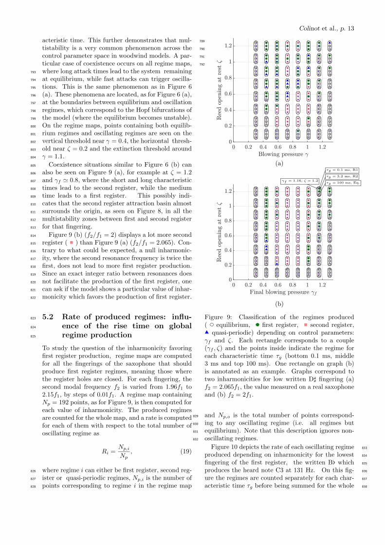
Focusing on Figure 9 (a), several features can be de- 784
scribed, and recognized from the situations explored 785
in Section 4 with a fixed ζ. Coexistence regions can be 786
noticed on most of the map, with a given (γf , ζ) cou- 787
ple leading to different regimes depending on the char- 788
Colinot et al., p. 13
acteristic time. This further demonstrates that mul- 789
tistability is a very common phenomenon across the 790
control parameter space in woodwind models. A par- 791
ticular case of coexistence occurs on all regime maps, 792
where long attack times lead to the system remaining793
at equilibrium, while fast attacks can trigger oscilla-794
tions. This is the same phenomenon as in Figure 6795
(a). These phenomena are located, as for Figure 6 (a),796
at the boundaries between equilibrium and oscillation797
regimes, which correspond to the Hopf bifurcations of798
the model (where the equilibrium becomes unstable).799
On the regime maps, points containing both equilib-800
rium regimes and oscillating regimes are seen on the801
vertical threshold near γ = 0.4, the horizontal thresh-802
old near ζ = 0.2 and the extinction threshold around803
γ = 1.1.804
Coexistence situations similar to Figure 6 (b) can805
also be seen on Figure 9 (a), for example at ζ = 1.2806
and γf ' 0.8, where the short and long characteristic807
times lead to the second register, while the medium808
time leads to a first register. This possibly indi-809
cates that the second register attraction basin almost810
surrounds the origin, as seen on Figure 8, in all the811
multistability zones between first and second register812
for that fingering.813
Figure 9 (b) (f2/f1 = 2) displays a lot more second814
register ( ) than Figure 9 (a) (f2/f1 = 2.065). Con-815
trary to what could be expected, a null inharmonic-816
ity, where the second resonance frequency is twice the817
first, does not lead to more first register production.818
Since an exact integer ratio between resonances does819
not facilitate the production of the first register, one820
can ask if the model shows a particular value of inhar-821
monicity which favors the production of first register.822
5.2 Rate of produced regimes: influ-823
ence of the rise time on global824
regime production825
To study the question of the inharmonicity favoringfirst register production, regime maps are computedfor all the fingerings of the saxophone that shouldproduce first register regimes, meaning those wherethe register holes are closed. For each fingering, thesecond modal frequency f2 is varied from 1.96f1 to2.15f1, by steps of 0.01f1. A regime map containingNp = 192 points, as for Figure 9, is then computed foreach value of inharmonicity. The produced regimesare counted for the whole map, and a rate is computedfor each of them with respect to the total number ofoscillating regime as
Ri =Np,iNp
, (19)
where regime i can either be first register, second reg-826
ister or quasi-periodic regimes, Np,i is the number of827
points corresponding to regime i in the regime map828
(a)τg = 0.1 ms, R1
τg = 3.2 ms, R2
τg = 100 ms, Eq.γf = 1.16, ζ = 1.2
(b)
Figure 9: Classification of the regimes produced( equilibrium, first register, second register,
quasi-periodic) depending on control parameters:γf and ζ. Each rectangle corresponds to a couple(γf , ζ) and the points inside indicate the regime foreach characteristic time τg (bottom 0.1 ms, middle3 ms and top 100 ms). One rectangle on graph (b)is annotated as an example. Graphs correspond totwo inharmonicities for low written D] fingering (a)f2 = 2.065f1, the value measured on a real saxophoneand (b) f2 = 2f1.
and Np,o is the total number of points correspond-829
ing to any oscillating regime (i.e. all regimes but830
equilibrium). Note that this description ignores non-831
oscillating regimes.832
Figure 10 depicts the rate of each oscillating regime 833
produced depending on inharmonicity for the lowest 834
fingering of the first register, the written B[ which 835
produces the heard note C3 at 131 Hz. On this fig- 836
ure the regimes are counted separately for each char- 837
acteristic time τg before being summed for the whole 838

Colinot et al., p. 14
map to produce an averaged rate. On the averaged 839
rate, optimal points are highlighted by triangles, cor- 840
responding to the maximum of first register and min- 841
imum of second register produced, respectively. Both 842
appear for values slightly above f2/f1 = 2. The inhar-843
monicity values maximizing first register production844
do not correspond to exactly harmonic resonances,845
but a second resonance slightly higher than the oc-846
tave of the first. The proportion of quasi-periodic847
regimes is also displayed on the figure. Note that848
inharmonicity values around two lead to less quasi-849
periodic regimes, which is corroborated by existing850
results [24, 23]. On Figure 10, it can be seen that the851
region of low rate of production of the second register852
for f2/f1 between 2.05 and 2.09 almost coincides with853
a region of high rate of production of quasi-periodic854
regimes, for f2/f1 between 2.06 and 2.1. In this case,855
minimizing second register production seems to favor856
the production of quasi-periodic regimes.857
Figure 10 shows that ignoring multistability, by858
using only one value of characteristic time, could859
have lead to conclusions similar to those drawn with860
production rates averaged over several characteristic861
times. Indeed, all the characteristic times yield qual-862
itatively similar production rates. However, this is863
not always the case, and Figure 11 shows two exam-864
ples where neglecting multistability and studying only865
one characteristic time can lead to biased conclusions.866
Figure 10: Rate of produced regimes (Eq. (19)) forwritten low B[ fingering. Green: first register, red:second register, blue: quasi-periodic. Linestyles in-dicate the characteristic time. Dotted: τg = 0.1 ms,dash-dot: τg = 3.2 ms, dashed: τg = 100 ms, solid:averaged rate. An upward triangle marks the maxi-mum first register averaged rate, a downward trianglemarks the minimum second register rate.
For the D] fingering (Figure 11 (a)), one can see867
that depending on the chosen increase duration τg the868
production ratio varies greatly (from 20% to 60%). If869
any quantitative interpretation is to be expected from870
these results, it can be changed dramatically depend-871
ing on the chosen attack time. Notice that the lowest872
rate of first register corresponds to the longest attack873
time τg = 100 ms. Figure 9 shows that the first regis-874
ter regimes are produced on the edges of the zone of875
oscillation, in a multistability region between the first 876
register and the equilibrium. The longest attack times 877
in this region tend not to lead to a first register, but 878
instead to an equilibrium due to its attraction basin 879
surrounding the origin (see for instance Figure 7 (c) or 880
multimedia file Supp1.mp4). Figure 11 (b) shows the 881
results for the written D fingering. This case exhibits 882
an outlier: the shortest attack time yields a optimal 883
inharmonicity value of 2.08, whereas the others point 884
to 2.04. In this case, considering several attack times 885
is a way to smooth out outliers due to a particular 886
value of the attack time. 887
Note that Graph 11 (b) can also be subject to an 888
interesting interpretation in terms of musician control 889
strategies: the fact that certain attack time values 890
seem to markedly decrease the rate of production of a 891
certain regime could be used by the musician to avoid 892
producing it. 893
5.3 Inharmonicity of the saxophone894
In this section, the optimal inharmonicity in terms of895
regime production is studied for the seven lowest fin-896
gerings of the instrument. Higher fingerings are not897
represented because they add no relevant information:898
first register regime production rates are close to 100%899
for all the studied inharmonicity values. This corre-900
sponds to the saxophonists’ experience that the high901
notes of the instrument’s first register are often eas-902
ier to produce than the low notes, and to the fact903
that the first impedance peak is much higher than904
the others on the high fingerings [14]. The optimums905
are compared with the inharmonicity value measured906
on the saxophone on which the model is based. Fig-907
ure 12 summarizes the production ratios for all the908
fingerings. The optimal inharmonicity seems to vary909
across the fingerings. It is always greater than two:910
null inharmonicity does not favor first register pro-911
duction on the low fingerings of the saxophone. The912
two optimums are close to the measured inharmonic-913
ity. Additionally, the trend is respected, with optimal914
and measured harmonicities increasing for higher fin-915
gerings. Note that the optimum for the E fingering916
is very far from the measured inharmonicity, but the917
production ratios are almost constant. Overall, the918
simulation shows that the most first register and least919
second register is produced by the model for values of920
inharmonicity near those measured on the saxophone.921
This result sheds some light on the empirical choice of922
the acoustical properties on the saxophone. Indeed, if923
the inharmonicity was far from the values observed on924
saxophones, the model predicts more second register925
would be produced. This effect is arguably undesir-926
able. However, this choice comes with a compromise,927

Colinot et al., p. 15
(a)
(b)
Figure 11: Rate of first register regime (Eq. (19)) pro-duced for (a) written low D] fingering and (b) writtenlow D fingering. Linestyles indicate the characteristictime. Dotted: τg = 0.1 ms, dash-dot: τg = 3.2 ms,dashed: τg = 100 ms, solid: averaged rate. An up-ward triangle marks the maximums of first registerrates.
as it also favors quasi-periodic regime production (see928
Figure 10), which are a known issue in low saxophone929
fingerings.930
6 Conclusion931
In the studied saxophone model, stable regimes coex-932
ist throughout large regions in the musician control933
parameter space. Thus, even an exhaustive descrip-934
tion of the stability or instability of each oscillating935
regime in the control parameter space is only an in-936
complete answer, as it doesn’t suffice to predict which937
regime emerges in these multistability zones. In par-938
ticular, in the event that the attraction basin of a sta-939
ble regime proves too small or unattainable by the mu-940
sician, this regime should be considered unreachable,941
almost like an unstable regime. This work demon-942
Figure 12: Rate of produced regimes for the lowest fin-gerings of the alto saxophone (written pitch). Green:first register, red: second register. An upward trian-gle marks the maximum first register averaged rate,a downward triangle marks the minimum second reg-ister rate. Vertical lines mark the measured inhar-monicity values.
strates that saxophone regime stability is a nuanced943
topic.944
An adapted combination of two radically different945
numerical methods provides a more complete descrip-946
tion of the model’s behavior: the stability study per-947
formed by harmonic balance method is completed by948
time-domain synthesis, which quantifies multistabil- 949
ity by outlining the attraction basin of each regime. 950
A varying control scenario explores which regime is 951
produced in multistability zones, with the advantage 952
that it can be tied to plausible musician actions. How- 953
ever, a varying control scenario only provides a very 954
partial view of the attraction basins, and its results 955
deserve to be explicited by representing the attraction 956
basins in the phase space using different initial condi- 957
tions. Dedicated experimental work, out of the scope 958
of this paper, could help design more realistic control 959
scenarios. 960
Accounting for multistability, the study of synthe- 961
sized regimes may explain an acoustical choice made 962
by instruments makers: the inharmonicity of the sax- 963
ophone. An integer ratio between the first and second 964
resonance frequencies does not favor the production 965
of first register. Note that this result adds nuance 966
one of Benade’s guidelines stating that an oscillation 967
Colinot et al., p. 16
is favored if the impedance is large at its fundamental 968
and its harmonic frequencies [4]. This work shows 969
that competition between registers also comes into 970
play, depending on more than solely the impedance 971
magnitude at the playing frequency and its harmon- 972
ics. Instead, an integer ratio between the first and 973
second resonance frequencies tends to favor the pro-974
duction of second register, which is arguably unde-975
sirable for a first register fingering. Carefully tuned976
inharmonic resonances, where the second frequency977
is higher than twice the first, can lead to more first978
register production. The optimal inharmonicity value979
found on the model is close to harmonicities measured980
on saxophone resonators. This result provides an a981
posteriori interpretation of the acoustical characteris-982
tics of the saxophone, as chosen empirically by instru-983
ment makers, as the acoustical characteristic leading984
to easier production of the first register. Such results985
are among the first steps towards applying numerical986
simulations as predictive tools to estimate playability987
in instrument design.988
Acknowledgments989
The authors would like to thank Erik Petersen for cor-990
recting the English. This work has been carried out in991
the framework of the Labex MEC (ANR-10-LABEX-992
0092) and of the A*MIDEX project (ANR-11-IDEX-993
0001-02), funded by the Investissements d’Avenir994
French Government program managed by the French995
National Research Agency (ANR). This study has996
been supported by the French ANR LabCom LIAMFI997
(ANR-16-LCV2-007-01).998
References999
[1] J. Backus, Vibrations of the reed and the air1000
column in the clarinet, The Journal of the Acous-1001
tical Society of America, 33 (1961), pp. 806–809.1002
[2] , Small-vibration theory of the clarinet, The1003
Journal of the Acoustical Society of America, 351004
(1963), pp. 305–313.1005
[3] A. H. Benade, Fundamentals of musical1006
acoustics, Courier Corporation, 1990.1007
[4] A. H. Benade and D. Gans, Sound production1008
in wind instruments, Annals of the New York1009
Academy of Sciences, 155 (1968), pp. 247–263.1010
[5] B. Bentvelsen and A. Lazarus, Modal and1011
stability analysis of structures in periodic elastic1012
states: application to the ziegler column, Nonlin-1013
ear Dynamics, 91 (2018), pp. 1349–1370.1014
[6] B. Bergeot, A. Almeida, C. Vergez,1015
and B. Gazengel, Prediction of the dynamic1016
oscillation threshold in a clarinet model with a1017
linearly increasing blowing pressure, Nonlinear1018
Dynamics, 73 (2013), pp. 521–534.1019
[7] W. Beyn, A. Champneys, E. Doedel,1020
W. Govarets, U. Kuznetsov, A. Yu, and1021
B. Sandstede, Handbook of Dynamical1022
Systems (Vol 2), chapter Numerical 1023
Continuation, and Computation of Normal 1024
Forms, Elsevier, 2002. 1025
[8] S. Bilbao, A. Torin, and V. Chatziioan- 1026
nou, Numerical modeling of collisions in musical 1027
instruments, Acta Acustica united with Acus- 1028
tica, 101 (2015), pp. 155–173. 1029
[9] H. Bouasse, Instruments a vent, Impr. Dela- 1030
grave, 1929. 1031
[10] S. Brezetskyi, D. Dudkowski, and T. Kap- 1032
itaniak, Rare and hidden attractors in van der 1033
pol-duffing oscillators, The European Physical 1034
Journal Special Topics, 224 (2015), pp. 1459– 1035
1467. 1036
[11] D. M. Campbell, J. Gilbert, and A. My- 1037
ers, The Science of Brass Instruments, Springer, 1038
2020. 1039
[12] A. Chaigne and J. Kergomard, Acoustique 1040
des instruments de musique (Acoustics of musical 1041
instruments), Belin, 2008. 1042
[13] V. Chatziioannou and M. van Walstijn, 1043
Estimation of clarinet reed parameters by inverse 1044
modelling, Acta Acustica united with Acustica, 1045
98 (2012), pp. 629–639. 1046
[14] J.-M. Chen, J. Smith, and J. Wolfe, 1047
Saxophone acoustics: introducing a compendium 1048
of impedance and sound spectra, Acoustics Aus- 1049
tralia, 37 (2009). 1050
[15] B. Cochelin and C. Vergez, A high order 1051
purely frequency-based harmonic balance 1052
formulation for continuation of periodic 1053
solutions, Journal of sound and vibration, 1054
324 (2009), pp. 243–262. 1055
[16] T. Colinot, Numerical simulation of woodwind 1056
dynamics: investigating nonlinear sound 1057
production behavior in saxophone-like 1058
instruments, PhD thesis, Aix-Marseille Uni- 1059
versite, 2020. 1060
[17] T. Colinot, P. Guillemain, C. Vergez, 1061
J.-B. Doc, and P. Sanchez, Multiple 1062
two-step oscillation regimes produced by the alto 1063
saxophone, The Journal of the Acoustical Society 1064
of America, 147 (2020), pp. 2406–2413. 1065
[18] T. Colinot, L. Guillot, C. Vergez, 1066
P. Guillemain, J.-B. Doc, and B. Coche- 1067
lin, Influence of the “ghost reed” simplification 1068

Colinot et al., p. 17
of the bifurcation diagram of a saxophone model, 1069
Acta Acustica united with Acustica, 105 (2019), 1070
pp. 1291–1294. 1071
[19] W. L. Coyle, P. Guillemain, J. Kergo-1072
mard, and J.-P. Dalmont, Predicting playing1073
frequencies for clarinets: A comparison between1074
numerical simulations and simplified analytical1075
formulas, The Journal of the Acoustical Society1076
of America, 138 (2015), pp. 2770–2781.1077
[20] J.-P. Dalmont, B. Gazengel, J. Gilbert,1078
and J. Kergomard, Some aspects of tuning1079
and clean intonation in reed instruments, Ap-1080
plied acoustics, 46 (1995), pp. 19–60.1081
[21] J.-P. Dalmont, J. Gilbert, and S. Ol-1082
livier, Nonlinear characteristics of single-reed1083
instruments: Quasistatic volume flow and reed1084
opening measurements, The Journal of the1085
Acoustical Society of America, 114 (2003),1086
pp. 2253–2262.1087
[22] J.-P. Dalmont and J. C. Le Roux, A new1088
impedance sensor for wind instruments, The1089
journal of the Acoustical Society of America, 1231090
(2008), pp. 3014–3014.1091
[23] J.-B. Doc and C. Vergez, Oscillation regimes1092
produced by an alto saxophone: Influence of the1093
control parameters and the bore inharmonicity,1094
The Journal of the Acoustical Society of Amer-1095
ica, 137 (2015), pp. 1756–1765.1096
[24] J.-B. Doc, C. Vergez, and S. Missoum,1097
A minimal model of a single-reed instrument1098
producing quasi-periodic sounds, Acta Acustica1099
united with Acustica, 100 (2014), pp. 543–554.1100
[25] V. Freour, H. Masuda, E. Tominaga,1101
Y. Tohgi, B. Cochelin, C. Vergez, et al.,1102
Numerical analysis and comparison of brass1103
instruments by continuation, in Proceedings of1104
the International Symposium on Musical Acous-1105
tics, 2019.1106
[26] J. Gilbert, J. Kergomard, and E. Ngoya,1107
Calculation of the steady-state oscillations of a1108
clarinet using the harmonic balance technique,1109
The journal of the Acoustical Society of America,1110
86 (1989), pp. 35–41.1111
[27] J. Gilbert, S. Maugeais, and C. Vergez,1112
From the bifurcation diagrams to the ease of1113
playing of reed musical instruments. a theoretical1114
illustration of the bouasse-benade prescription?,1115
in Proceedings of the International Symposium1116
on Musical Acoustics, 2019.1117
[28] A. Y. Gokhshtein, Self-vibration of finite1118
amplitude in a tube with a reed, in Soviet Physics1119
Doklady, vol. 24, 1979, p. 739.1120
[29] P. Guillemain, J. Kergomard, and1121
T. Voinier, Real-time synthesis of clarinet-like1122
instruments using digital impedance models, The1123
Journal of the Acoustical Society of America, 1124
118 (2005), pp. 483–494. 1125
[30] P. Guillemain, C. Vergez, D. Ferrand, 1126
and A. Farcy, An instrumented saxophone 1127
mouthpiece and its use to understand how 1128
an experienced musician plays, Acta Acustica 1129
united with Acustica, 96 (2010), pp. 622–634. 1130
[31] L. Guillot, B. Cochelin, and C. Vergez, 1131
A taylor series-based continuation method for 1132
solutions of dynamical systems, Nonlinear Dy- 1133
namics, (2019), pp. 1–19. 1134
[32] L. Guillot, A. Lazarus, O. Thomas, 1135
C. Vergez, and B. Cochelin, A purely 1136
frequency based floquet-hill formulation for 1137
the efficient stability computation of periodic 1138
solutions of ordinary differential systems, Non- 1139
linear Dynamics, – (2020 (submitted)), pp. ?–? 1140
[33] A. Guilloteau, P. Guillemain, J. Ker- 1141
gomard, and M. Jousserand, The effect of 1142
the size of the opening on the acoustic power 1143
radiated by a reed woodwind instrument, Journal 1144
of Sound and Vibration, 343 (2015), pp. 166–175. 1145
[34] T. Helie, N. Lopes, and R. Causse, 1146
Open-loop control of a robotized artificial mouth 1147
for brass instruments, The Journal of the Acous- 1148
tical Society of America, 131 (2012), pp. 3470– 1149
3470. 1150
[35] A. Hirschberg, J. Kergomard, and 1151
G. Weinreich, Mechanics of musical 1152
instruments, chapter 6 (J. Kergomard): 1153
Elementary considerations on reed-instrument 1154
oscillations, CISM courses and lectures, 355 1155
(1995), pp. 229–290. 1156
[36] A. Hirschberg, R. Van de Laar, 1157
J. Marrou-Maurieres, A. Wijnands, 1158
H. Dane, S. Kruijswijk, and A. Houtsma, 1159
A quasi-stationary model of air flow in the reed 1160
channel of single-reed woodwind instruments, 1161
Acta Acustica united with Acustica, 70 (1990), 1162
pp. 146–154. 1163
[37] T. Idogawa, T. Kobata, K. Komuro, and 1164
M. Iwaki, Nonlinear vibrations in the air column 1165
of a clarinet artificially blown, The Journal of 1166
the Acoustical Society of America, 93 (1993), 1167
pp. 540–551. 1168
[38] J. Kergomard, P. Guillemain, F. Silva, 1169
and S. Karkar, Idealized digital models for 1170
conical reed instruments, with focus on the 1171
internal pressure waveform, The Journal of 1172

Colinot et al., p. 18
the Acoustical Society of America, 139 (2016), 1173
pp. 927–937. 1174
[39] N. M. Krylov and N. N. Bogoliubov,1175
Introduction to non-linear mechanics, Princeton1176
University Press, 1949.1177
[40] Y. A. Kuznetsov, Elements of applied1178
bifurcation theory, vol. 112, Springer Science &1179
Business Media, 2013.1180
[41] A. Lazarus and O. Thomas, A1181
harmonic-based method for computing the1182
stability of periodic solutions of dynamical1183
systems, Comptes Rendus Mecanique, 3381184
(2010), pp. 510–517.1185
[42] N. Lopes, T. Helie, and R. Causse, Control1186
of an artificial mouth playing a trombone and1187
analysis of sound descriptors on experimental1188
data, in Proceedings of the Stockholm Music1189
Acoustics Conference 2013, 2013.1190
[43] I. R. Manchester, M. M. Tobenkin,1191
M. Levashov, and R. Tedrake, Regions of1192
attraction for hybrid limit cycles of walking1193
robots, IFAC Proceedings Volumes, 44 (2011),1194
pp. 5801–5806.1195
[44] T. Matsumoto, A chaotic attractor from chua’s1196
circuit, IEEE Transactions on Circuits and Sys-1197
tems, 31 (1984), pp. 1055–1058.1198
[45] C. McGinnis and C. Gallagher, The mode1199
of vibration of a clarinet reed, The Journal of1200
the Acoustical Society of America, 12 (1941),1201
pp. 529–531.1202
[46] A. Munoz Arancon, B. Gazengel, J.-1203
P. Dalmont, and E. Conan, Estimation of1204
saxophone reed parameters during playing, The1205
Journal of the Acoustical Society of America, 1391206
(2016), pp. 2754–2765.1207
[47] M. Nakhla and J. Vlach, A piecewise1208
harmonic balance technique for determination1209
of periodic response of nonlinear systems, IEEE1210
Transactions on Circuits and Systems, 23 (1976),1211
pp. 85–91.1212
[48] G. Pegna, R. Marrocu, R. Tonelli,1213
F. Meloni, and G. Santoboni, Experimental1214
definition of the basin of attraction for chua’s1215
circuit, International Journal of Bifurcation and1216
Chaos, 10 (2000), pp. 959–970.1217
[49] E. Petersen, P. Guillemain, J. Kergo-1218
mard, and T. Colinot, The effect of the1219
cutoff frequency on the sound production of1220
a clarinet-like instrument, The Journal of the1221
Acoustical Society of America, 145 (2019),1222
pp. 3784–3794.1223
[50] S. N. Rasband, Chaotic dynamics of nonlinear1224
systems, Courier Dover Publications, 2015.1225
[51] A. Schwab and M. Wisse, Basin of attraction 1226
of the simplest walking model, in Proceedings of 1227
the ASME design engineering technical confer- 1228
ence, vol. 6, 2001, pp. 531–539. 1229
[52] R. Seydel, Practical bifurcation and stability 1230
analysis, vol. 5, Springer Science & Business Me- 1231
dia, 2009. 1232
[53] F. Silva, Emergence des auto-oscillations dans 1233
un instrument de musique a anche simple, PhD 1234
thesis, Aix-Marseille Universite, 2009. 1235
[54] F. Silva, C. Vergez, P. Guillemain, 1236
J. Kergomard, and V. Debut, Moreesc: a 1237
framework for the simulation and analysis of 1238
sound production in reed and brass instruments, 1239
Acta Acustica united with Acustica, 100 (2014), 1240
pp. 126–138. 1241
[55] N. V. Stankevich, N. V. Kuznetsov, G. A. 1242
Leonov, and L. O. Chua, Scenario of the birth 1243
of hidden attractors in the chua circuit, Inter- 1244
national Journal of Bifurcation and Chaos, 27 1245
(2017), p. 1730038. 1246
[56] K. Takahashi, H. Kodama, A. Naka- 1247
jima, and T. Tachibana, Numerical study on 1248
multi-stable oscillations of woodwind single-reed 1249
instruments, Acta Acustica united with Acus- 1250
tica, 95 (2009), pp. 1123–1139. 1251
[57] S. Terrien, C. Vergez, and B. Fabre, 1252
Flute-like musical instruments: a toy model 1253
investigated through numerical continuation, 1254
Journal of sound and vibration, 332 (2013), 1255
pp. 3833–3848. 1256
[58] R. Tournemenne, J.-F. Petiot, B. Tal- 1257
gorn, M. Kokkolaras, and J. Gilbert, 1258
Brass instruments design using physics-based 1259
sound simulation models and surrogate-assisted 1260
derivative-free optimization, Journal of Mechan- 1261
ical Design, 139 (2017). 1262
[59] L. Wang, W. Lu, and T. Chen, Multistability 1263
and new attraction basins of almost-periodic 1264
solutions of delayed neural networks, IEEE 1265
Transactions on Neural Networks, 20 (2009), 1266
pp. 1581–1593. 1267
[60] T. A. Wilson and G. S. Beavers, Operating 1268
modes of the clarinet, The Journal of the Acous- 1269
tical Society of America, 56 (1974), pp. 653–658. 1270
[61] M. Wisse, A. L. Schwab, and F. C. van der 1271
Helm, Passive dynamic walking model with 1272
upper body, Robotica, 22 (2004), pp. 681–688. 1273
Colinot et al., p. 19
[62] M. Wisse, A. L. Schwab, R. Q. van der 1274
Linde, and F. C. van der Helm, How to 1275
keep from falling forward: Elementary swing leg 1276
action for passive dynamic walkers, IEEE Trans-1277
actions on robotics, 21 (2005), pp. 393–401.1278
List of Figures 1279
1 Measured input impedance (solid) and 1280
modal reconstruction (dashed) for the 1281
fingering D] of the alto saxophone. . 4 1282
2 Time-domain synthesized pressure sig- 1283
nal. (a) temporal envelope (black) and 1284
blowing pressure parameter γ (red). 1285
(b) Normalized spectrogram (dB) with 1286
regime names indicated (unstable ones 1287
between parentheses) : equilibrium 1288
(Eq.), second register, quasi-periodic 1289
and first register. The signal is ex- 1290
tracted from the same blowing pressure 1291
ramp as in Figure 4, between γ = 0.45 1292
and γ = 0.51 (at first occurrence of os- 1293
cillation). . . . . . . . . . . . . . . . . 4 1294
3 Bifurcation diagram obtained with 1295
harmonic balance method and numeri- 1296
cal continuation: L2-norm of the acous- 1297
tical pressure depending on the blow- 1298
ing pressure parameter γ for the low 1299
written D] fingering of an alto sax- 1300
ophone. Thick lines: stable solu- 1301
tion, thin lines: unstable solutions. 1302
Black: equilibrium, green: 1st regis- 1303
ter regimes, red: 2nd register regimes. 1304
Multistability zones are shaded: light 1305
yellow where 1st and 2nd register co- 1306
exist, darker gray for equilibrium and 1307
1st register. Blue circles specify the lo- 1308
cation of bifurcations. Vertical black 1309
lines correspond to those in Figure 6 1310
(c), and (from left to right) to phase 1311
diagrams 7 (a), (b) and (c). . . . . . . 6 1312
4 L2-norm of the time-domain synthesis 1313
signal (dark blue line) for control sce- 1314
nario number one, a ramp of the blow- 1315
ing pressure parameter γ from 0 to 2 1316
and down, overlaid with the bifurca- 1317
tion diagram of Figure 3 (thick stable 1318
solutions and thin unstable solutions, 1319
of the first register in green and second 1320
register in red). Solid dark blue line in- 1321
dicates the first part of the signal (in- 1322
creasing γ) and dashed dark blue line 1323
the second (decreasing γ). . . . . . . 7 1324
5 Four examples of blowing pressure vari- 1325
ations in control scenario number two, 1326
as described by Eq. (17), for γf = 0.4 1327
and 0.6 and τg = τ[1]g = 10 ms and 1328
τ[2]g = 20 ms. . . . . . . . . . . . . . . 8 1329

Colinot et al., p. 20
6 Classification of the steady-state1330
regimes produced with control sce-1331
nario number two, depending on the1332
blowing pressure transient parameters:1333
final value γf and characteristic time1334
τg. Multistability zones (deduced from1335
Figure 3): (a) equilibrium and first1336
register (b) first register and second1337
register (c) all three regime types.1338
Blue triangles indicate quasi-periodic1339
regimes. The horizontal line on graph1340
(b) shows τ = 1/f1. The vertical1341
lines highlight the γ values of phase1342
diagrams in Figure 7 and 8. . . . . . . 91343
7 Projection of the attraction basins ob-1344
tained with control scenario number1345
three . Large dots are initial condi-1346
tions, small dots are points the syn-1347
thesis goes through. The dots’ colors1348
indicate the final regime they lead to1349
(black: equilibrium, green: first regis-1350
ter, red: second register). Blue lines1351
represent the limit cycles. The small1352
one on the inside is the first register1353
and the one on the outside is the sec-1354
ond register. The blowing pressure γ1355
is (a) 1, (b) 1.1, (c) 1.2 (highlighted in1356
figures 6 and 3). . . . . . . . . . . . . 111357
8 Attraction basins (dots) and limit cy-1358
cles (lines) in a 3D projection of the1359
phase space obtained with control sce-1360
nario number three for different blow-1361
ing pressures γ. Black: equilibrium,1362
green: first register, red: second reg-1363
ister, blue: quasi-periodic. . . . . . . 121364
9 Classification of the regimes produced1365
(equilibrium, first register, second reg-1366
ister, quasi-periodic) depending on1367
control parameters: γf and ζ. Each1368
rectangle corresponds to a couple1369
(γf , ζ) and the points inside indicate1370
the regime for each characteristic time1371
τg (bottom 0.1 ms, middle 3 ms and top1372
100 ms). One rectangle on graph (b) is1373
annotated as an example. Graphs cor-1374
respond to two inharmonicities for low1375
written D] fingering (a) f2 = 2.065f1,1376
the value measured on a real saxo-1377
phone. (b) f2 = 2f1. . . . . . . . . . . 131378
10 Rate of produced regimes (Eq. (19)) 1379
for written low B[ fingering. Green: 1380
first register, red: second register, blue: 1381
quasi-periodic. Linestyles indicate the 1382
characteristic time. Dotted: τg = 1383
0.1 ms, dash-dot: τg = 3.2 ms, dashed: 1384
τg = 100 ms, solid: averaged rate. An 1385
upward triangle marks the maximum 1386
first register averaged rate, a down- 1387
ward triangle marks the minimum sec- 1388
ond register rate. . . . . . . . . . . . 14 1389
11 Rate of first register regime (Eq. (19)) 1390
produced for (a) written low D] fin- 1391
gering and (b) written low D finger- 1392
ing. Linestyles indicate the character- 1393
istic time. Dotted: τg = 0.1 ms, dash- 1394
dot: τg = 3.2 ms, dashed: τg = 100 ms, 1395
solid: averaged rate. An upward trian- 1396
gle marks the maximums of first regis- 1397
ter rates. . . . . . . . . . . . . . . . . 14 1398
12 Rate of produced regimes for the lowest 1399
fingerings of the alto saxophone (writ- 1400
ten pitch). Green: first register, red: 1401
second register. An upward triangle 1402
marks the maximum first register aver- 1403
aged rate, a downward triangle marks 1404
the minimum second register rate. Ver- 1405
tical lines mark the measured inhar- 1406
monicity values. . . . . . . . . . . . . 15 1407
List of Tables 1408
1 Parameters of the numerical model: 1409
musician control parameters γ and ζ, 1410
reed parameters qr and ωr, contact pa- 1411
rameter Kc and parameters inherent to 1412
the numerical implementation η, Nm 1413
and H. . . . . . . . . . . . . . . . . . . 3 1414
2 Modal parameters for the fingering D] 1415
of the alto saxophone. . . . . . . . . . 4 1416


![Wave heave energy conversion using modular multistability Energy/wave heave modualr... · 2014-06-29 · Wave heave energy conversion using modular multistability ... [3–6], while](https://img.pdfslide.us/doc/110x75/5e3515fd28986c6ed857f62f/wave-heave-energy-conversion-using-modular-energywave-heave-modualr-2014-06-29.jpg)