Embed Size (px)
Citation preview
Department of Electrical and
Computer Engineering
Lisbon, Portugal
Department of Electronics and
Information Technology Warsaw, Poland
Multiservice Traffic Analysis
in Mobile Broadband Systems
Krzysztof Marek Platek
Lisbon, Portugal
October 2000


i
Under the supervision of:
Luis M. Correia
Department of Electrical and Computer Engineering
Instituto Superior Tecnico
Technical University of Lisbon

ii

iii
"It is dangerous to put limits on wireless" Guglielmo Marconi (1932)

iv

v
Acknowledgements
There are plenty of persons who took place in my life here in Lisbon to whom I would
like at least to leave my thanks. Even if I forget somebody now, for sure I will remind them
during future recollections.
Special thanks to Prof. Luis Correia for the time dedicated to me, for great working
atmosphere, for making me smile, for excellent comparisons and approaches and for the big
amount of new knowledge given to me (not only the one that concerns this project).
Also special thanks to the Ph.D. student Fernando Velez for his patience, advises, help
and materials presented to me in each step of my work in IST.
Many thanks to my tutor from the Warsaw University of Technology, dr Tomasz
Kosilo, for waking up my wireless soul and for leading my studies in Poland.
Thanks to Fundacja Wspierania Rozwoju Radiokomunikacji i Technik
Multimedialnych for supporting and sponsoring my existence in Portugal.
Many thanks to D. Isabel and D. Olivia for taking care of my needs during my stay at
IST.
Thanks to my parents for everything they did for me during my whole life.
Thanks to Malgosia Kozera for reminding me of my Polish roots each day – You don't
know how much You were important to me while You played in my life Wajdelota's and
Aldona's role at the same time.
Many thanks to Robert Szczygielski, his mother Teresa and my friends from "ERA
GSM": Krzysztof Kucharski and Michal Zajaczkowski – without You perhaps I could not be
here.

vi
Thanks to my friends from Ericsson Poland and Nokia Poland for their interest in my
life and for supplying me with materials, specially to Beata Bojarska for keeping me in touch
with the polish language.
Luca my friend: for You I'm specially thankful. It is not easy to find a true friend in a
stranger land – You are to me like a brother.
Plenty of thanks to my friends from the laboratory: Rui, Pedro, Hugo, Ze, Joao,
Miguel and Juan for a time and work we spent and did together.
Thanks to Miguel and Manuel, my Spanish friends, who guided me at my first steps in
Lisbon.
Thanks to Teresa and Chiara for their acceptance of the Polish mentality while we
lived together.
Thanks to Johny and Johan for common journeys, trips and discovers.
Thanks to Joao Mestre with whom I shared the room and the other things in the IST
Residence. Thanks to all my neighbours from the Residence for the wonderful atmosphere as
well.
Thanks to Sofia, Gabi, Margerida, Maria, Ana, Emy, Jennifer, Mª Joao for great the
party we participated together.
Thanks to all the Italian "mafia" I met here, for their friendship and company.
vii
Table of contents
ACKNOWLEDGEMENTS v
TABLE OF CONTENTS vii
LIST OF FIGURES ix
LIST OF TABLES xi
LIST OF ACRONYMS xiii
LIST OF SYMBOLS xv
1. INTRODUCTION 1
2. BROADBAND SERVICES & APPLICATIONS 5
2.2. Broadband Service Classification 5
2.3. Mobile Applications and Bandwidth Evolution 11
3. TRAFFIC THEORY BASIS 19
3.1. Introduction 19
3.2. Intensity and Units of Traffic 19
3.3. Birth and Death Process 20
3.4. Basic Aspects of Traffic Modelling 21
3.4.1. Bursty and Renewal Traffic 21
3.4.2. Poisson Process 23
3.4.3. Bernoulli Process 24
3.4.4. Markov and Markov-Renewal Traffic Models 25
3.4.5. Erlang Models 30
3.4.6. Markov Based Traffic Modelling in Mobile Systems 34
3.4.7. Other Models 41
3.5. Multiservice Traffic Modelling 42
3.5.1. Markov Modulated Traffic Models 42
3.5.2. Bernoulli – Poisson – Pascal Process 44
4. SYSTEM PERFORMANCE SIMULATION 53
4.1. Introduction 53
4.2. Application Characteristics and Simulation Parameters 53
4.3. Impact of Mobility 101
5. CONCLUSIONS 103
6. APPENDIX A 107

viii
ix
List of Figures
Figure 1.1 Mobile Broadband System as extension to B-ISDN 2
Figure 2.1 Basic service components (extracted from [VeCo00]) 7
Figure 2.2 Classification of services according to ITU-T I.211 (extracted from
[VeCo00])
8
Figure 2.3
Forecasted traffic growth of data in mobile networks as function of time,
extracted from [Beck00]
11
Figure 2.4 Mobile Systems Evolution 12
Figure 2.5 Comparison of Circuit Switched and Packet Switched modes 12
Figure 2.6 Systems evolution toward MBS 16
Figure 3.1 State transition diagram for one dimensional birth death process 20
Figure 3.2 Areas of bursty and bandwidth consuming by applications extracted from
[EN7499]
22
Figure 3.3 Superposition of Poisson processes 23
Figure 3.4
Probability of k system channels being busy (k simultaneous calls) using
Poisson distribution for A=10 Erlang and A=28 Erlang
24
Figure 3.5
Probability of k system channels being busy (k simultaneous calls) using
Bernoulli distribution for A=10 Erlang and A=28 Erlang
25
Figure 3.6 On-Off Model 26
Figure 3.7 Interrupted Poisson Process (IPP) 26
Figure 3.8 M/M/1 queue as an example of single server system 27
Figure 3.9 Average queue length for M/M/1 model as a function of traffic intensity 28
Figure 3.10 M/G/1 Queue 29
Figure 3.11 Average queue length for M/G/1 model as a function of traffic intensity 30
Figure 3.12 Probability of blocking ( GOS ) for: C=30 and C=100 according to
Erlang B
32
Figure 3.13 The Erlang C formula probability of a call being delayed ( t >0 ) for:
C=30 and C=100
33
Figure 3.14
The Erlang C formula probability of a call being delayed for delaying
time t and given C=30; T=180[s]
34
Figure 3.15 Presentation of mobility during call with cell dwell time 35
Figure 3.16 Terminal mobility and dwell time in street micro cells 36
x
Figure 3.17
State transition diagram for mobile environments with C total channels,
and g dedicated for guards
36
Figure 3.18
Probability of blocking as function of dedicated channels for guards with
given Ah = 4 Erlang
38
Figure 3.19 Handover failed probability as function An for given Ah = 4 Erlang and g
as on chart
39
Figure 3.20 Call dropping probability as function of terminal average velocity 40
Figure 3.21 Drop call probability as function of cell radius 41
Figure 3.22 MMPP process 43
Figure 3.23 MMPP process arrival rates for voice/data common abilities usage 43
Figure 3.24 MMFM process 44
Figure 3.25 BPP model for K applications 45
Figure 3.26 Markov chain model of a BPP process, extracted from [AwVl96] 45
Figure 3.27 Service components activation 49
Figure 3.28 Service components activation according to Bernoulli model, extracted
from [Vele99]
50
Figure 4.1 Simulator input and output parameters 54
Figure 4.2 Service components Blocking Probability in BCC environment 60
Figure 4.3 Service components Blocking Probability in URB environment 64
Figure 4.4 Service components Blocking Probability in ROA environment 68
Figure 4.5 Service components Blocking Probability in BCC environment for TDD
Mode
74
Figure 4.6 Service components Blocking Probability in URB environment for TDD
Mode
78
Figure 4.7 Service components Blocking Probability in ROA environment for TDD
Mode
82
Figure 4.8 Service components Blocking Probability in Stadium environment 96
Figure A.1 Service components Blocking Probability in BCC environment 108
Figure A.2 Service components Blocking Probability in URB environment 120
Figure A.3 Service components Blocking Probability in ROA environment 128
xi
List of Tables Table 1.1 MBS objectives 3
Table 2.1 Example of applications with different information types and delivery
requirements (extracted from [Kwok95])
6
Table 2.2 B-ISDN applications and their requirements (extracted from [VeCo00]) 9
Table 2.3 Phase 2 user available bandwidth. 13
Table 2.4 Phase 2+ user available bandwidth 13
Table 2.5 Phase 3 user available data rates [NaBK00] 14
Table 2.6 UMTS applications and their peak bit rates (extracted from [VeCo00]). 15
Table 2.7 MBS applications and bandwidths (extracted from [VeCo00]) 17
Table 3.1 MBS Services characteristics (extracted from [Vele98]) 29
Table 3.2 Scenarios of mobility characteristics [VeCo98] 36
Table 4.1 Main MBS applications transmission parameters 55
Table 4.2 Average duration and proportion of application users in different
scenarios
55
Table 4.3 Number of 384 kbit/s channels available in a cell for different scenarios 56
Table 4.4 Service components and their bandwidth request 56
Table 4.5 Parameter n j/k for uplink 57
Table 4.6 Parameter j/k for uplink 57
Table 4.7 Parameter n j/k for downlink 58
Table 4.8 Parameter j/k for uplink 58
Table 4.9 Applications contributions for c1 and AF for different scenarios 72
Table 4.10 Number of channels used for TDD mode analysis 73
Table 4.11 Numbers of served component BAS users in BCC environment 86
Table 4.12 Numbers of served component MED1 users in BCC environment 86
Table 4.13 Numbers of served component MED2 users in BCC environment 86
Table 4.14 Numbers of served component MED3 users in BCC environment 87
Table 4.15 Numbers of served component HDV users in BCC environment 87
Table 4.16 Numbers of served component HID users in BCC environment 87
Table 4.17 Numbers of served component BAS users in URB environment 87
Table 4.18 Numbers of served component MED1 users in URB environment 87
Table 4.19 Numbers of served component MED2 users in URB environment 87
xii
Table 4.20 Numbers of served component MED3 users in URB environment 88
Table 4.21 Numbers of served component HDV users in URB environment 88
Table 4.22 Numbers of served component HID users in URB environment 88
Table 4.23 Numbers of served component BAS users in ROA environment 88
Table 4.24 Numbers of served component MED1 users in ROA environment 88
Table 4.25 Numbers of served component MED2 users in ROA environment 88
Table 4.26 Numbers of served component MED3 users in ROA environment 89
Table 4.27 Numbers of served component HDV users in ROA environment 89
Table 4.28 Numbers of served component HID users in ROA environment 89
Table 4.29
Average applications service time and proportion of applications users for
Airport and Stadium environment
90
Table 4.30 Parameter n j/k for uplink in Stadium environment 91
Table 4.31 Parameter j/k for uplink in Stadium environment 91
Table 4.32 Parameter n j/k for downlink in Stadium environment 92
Table 4.33 Parameter j/k for downlink in Stadium environment 92
Table 4.34 Parameter n j/k for uplink in Airport environment 93
Table 4.35 Parameter j/k for uplink in Airport environment 93
Table 4.36 Parameter n j/k for downlink in Stadium environment 94
Table 4.37 Parameter j/k for downlink in Airport environment 94
Table 4.38 Data rates associated with applications for Airport and Stadium case 95
Table 4.39 Summary of the results 100
Table 4.40 Application mobility in BCC, URB and ROA environment proposal
(extracted from [VeCo00])
101
Table A.1 Scenarios considered in Appendix A 107
xiii
List of Acronyms
AAL: ATM Adaptation Layer
ABR: Available Bit Rate
Asy: Asymmetric
ATM: Asynchronous Transmission Mode
BCC: Business City Centre environment
BER: Bit Error Rate
BPP: Bernoulli Poisson Pascal process
CBR: Constant Bit Rate
CC: Conversational Class
CoS: Class of Service
CS: Circuit Switched
CSD: Circuit Switched Data
DSL: Digital Subscriber Line
DWDM: Dense Wave Division Multiple Access
EDGE: Enhanced Data for GSM Evolution
ETSI: European Telecommunications Standards Institute
FCFS: First Come First Served
FDD: Frequency Division Duplex
FDMA: Frequency Division Multiple Access
FIFO: First In First Out
FTP: File Transfer Protocol
GoS: Grade of Service
GPRS: General Packet Radio Service
GSM: Global System for Mobile communications
HIMM: High Interactive MultiMedia
HMM: High MultiMedia
HSCSD: High Speed Circuit Switched Data
IC: Interactive Class
IEEE: Institute of Electrical and Electronic Engineering
IMT-2000: International Mobile Telecommunications 2000
IP: Internet Protocol
IPP: Interrupted Poisson Process
xiv
ITU: International Telecommunication Union
MAC: Medium Access Control
MBS: Mobile Broadband Systems
MMM: Medium MultiMedia
NRT: Non Real Time
NTB: Non Time Based
PDF: Probability Density Function
PMF: Probability Marginal Function
PS: Packet Switched
QoS: Quality of Service
ROA: main Roads environment
RT: Real Time
S: Speech
SAP: Service Access Point
SD: Switched Data
SF: Spreading Factor
SM: Simple Messaging
STM: Synchronous Transfer Mode
Sym: Symmetric
TB: Time Based
TCP: Transmission Control Protocol
TD-CDMA: Time Division-Code Division Multiple Access
TDD: Time Division Duplex
TDMA: Time Division Multiple Access
TV: TeleVision
UBR: Unspecified Bit Rate
UMTS: Universal Mobile Telecommunication System
URB: Urban environment
UTRA: UMTS Terrestrial Radio Access
UTRAN: UMTS Terrestrial Radio Access Network
VBR-NRT Variable Bit Rate – Non Real Time
VBR-RT Variable Bit Rate – Real Time
WCDMA: Wideband Code Division Multiple Access
WWW: World Wide Web
xv
List of Symbols
-1 Time spent in On state
k BPP process parameter
j BPP process parameter
-1 Time spent in Off state
j Activation rate of service component j
k BPP process activation factor of application k
Velocity standard deviation
Average number of calls generated by user per time unit (arrival rate)
j\k Service component j used by application k arrival rate
j(nj) Time after the next arrival of class j customer's arrival when the system is in state
N(t) = n
k Application k arrival rate
Average service rate
k Average application k service rate
j\k Service component j used by application k service rate
The cell cross over rate
Service time distribution variance
[Rt] Standard deviation of interarrival time
Call duration time when mobility is considered
c Channel occupancy time in a cell when mobility is considered
h Cell dwell time when mobility is considered
n Jump times
A Total traffic intensity generated by system users
AF Asymmetry factor
Ah Traffic rate incoming from handover
aj Service component j data rates
Ak Traffic generated per free user and for each application k
An New arising in a cell traffic
Au Traffic intensity generated by user
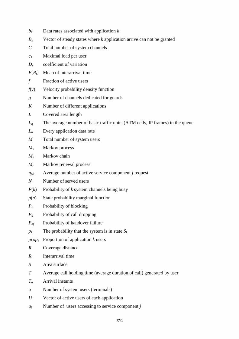
xvi
bk Data rates associated with application k
Bk Vector of steady states where k application arrive can not be granted
C Total number of system channels
c1 Maximal load per user
Dv coefficient of variation
E[Rt] Mean of interarrival time
f Fraction of active users
f(v) Velocity probability density function
g Number of channels dedicated for guards
K Number of different applications
L Covered area length
Lq The average number of basic traffic units (ATM cells, IP frames) in the queue
Lu Every application data rate
M Total number of system users
Mv Markov process
Mn Markov chain
Mr Markov renewal process
nj\k Average number of active service component j request
Nu Number of served users
P(k) Probability of k system channels being busy
p(n) State probability marginal function
Pb Probability of blocking
Pd Probability of call dropping
Phf Probability of handover failure
pk The probability that the system is in state Sk
propk Proportion of application k users
R Coverage distance
Rt Interarrival time
S Area surface
T Average call holding time (average duration of call) generated by user
Tn Arrival instants
u Number of system users (terminals)
U Vector of active users of each application
uj Number of users accessing to service component j
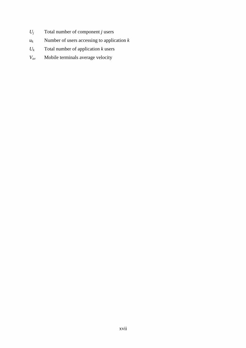
xvii
Uj Total number of component j users
uk Number of users accessing to application k
Uk Total number of application k users
Vav Mobile terminals average velocity
1
1 Introduction
Mobile communications systems are becoming an important part of people everyday's
life all around the world. Today's second generation (2G) cellular networks provide services
to customers using mobile terminals through the use of advanced technologies. As 2G
systems use digital technology, in contrast to the first generation ones, they are very
successful world-wide in providing high quality voice services to users. Thanks to systems
standardisation (e.g. GSM 900/1800 or IS 136) the ability to roam around the globe and
communicate using handheld terminals became reality, hence customer pool is increasing
faster than it was expected. Increasingly, those users will want to use a wireless access not
only for voice communication. However these successful today 2G systems are limited in
maximum data rate, thus the capabilities of cellular networks have to be improved. The High
Speed Circuit Switched Data (HSCSD) and General Packet Radio Service (GPRS) are an
actual user bit rate evolution in existing digital mobile networks that lead to high bandwidths,
up to 470 kbit/s in Enhanced Data Rates for GSM Evolution (EDGE).
More advanced services than current voice and low data rate services are foreseen.
Low and high definition video service components with high bandwidth demand are required
for new arising multimedia services. According to the UMTS Forum, in 2010 about 60 % of
traffic in Europe will be created by mobile multimedia applications. This is the background to
the new third generation (3G) wireless systems demand. The bit rate up to 2 Mbit/s per user is
assumed for the European 3G system – Universal Mobile Telecommunication System
(UMTS). Nevertheless future multimedia services will range from low (~ 0.5 Mbit/s) to high
user data rates (155 Mbit/s per user is foreseen). It is already well known that currently
developed 3G systems are not able to fulfil these expectations, due not only to their bit rate
but also to mobility limitations and packet switching (for high bit rate services) nature.
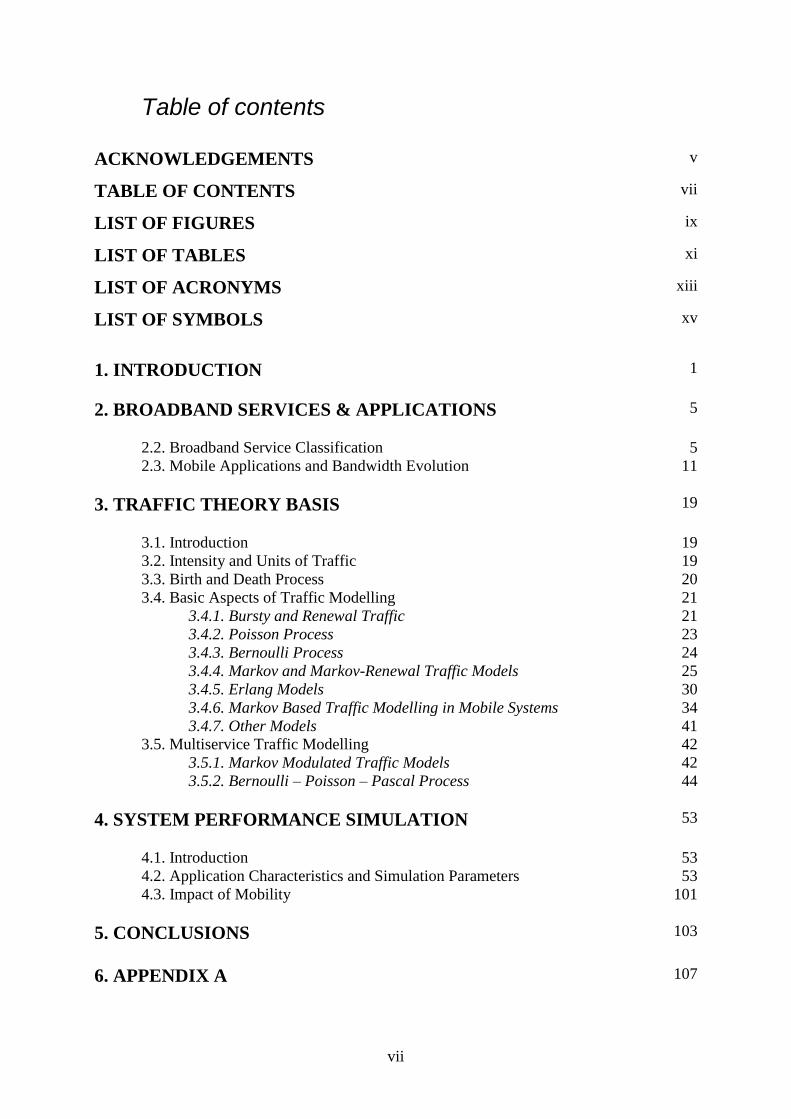
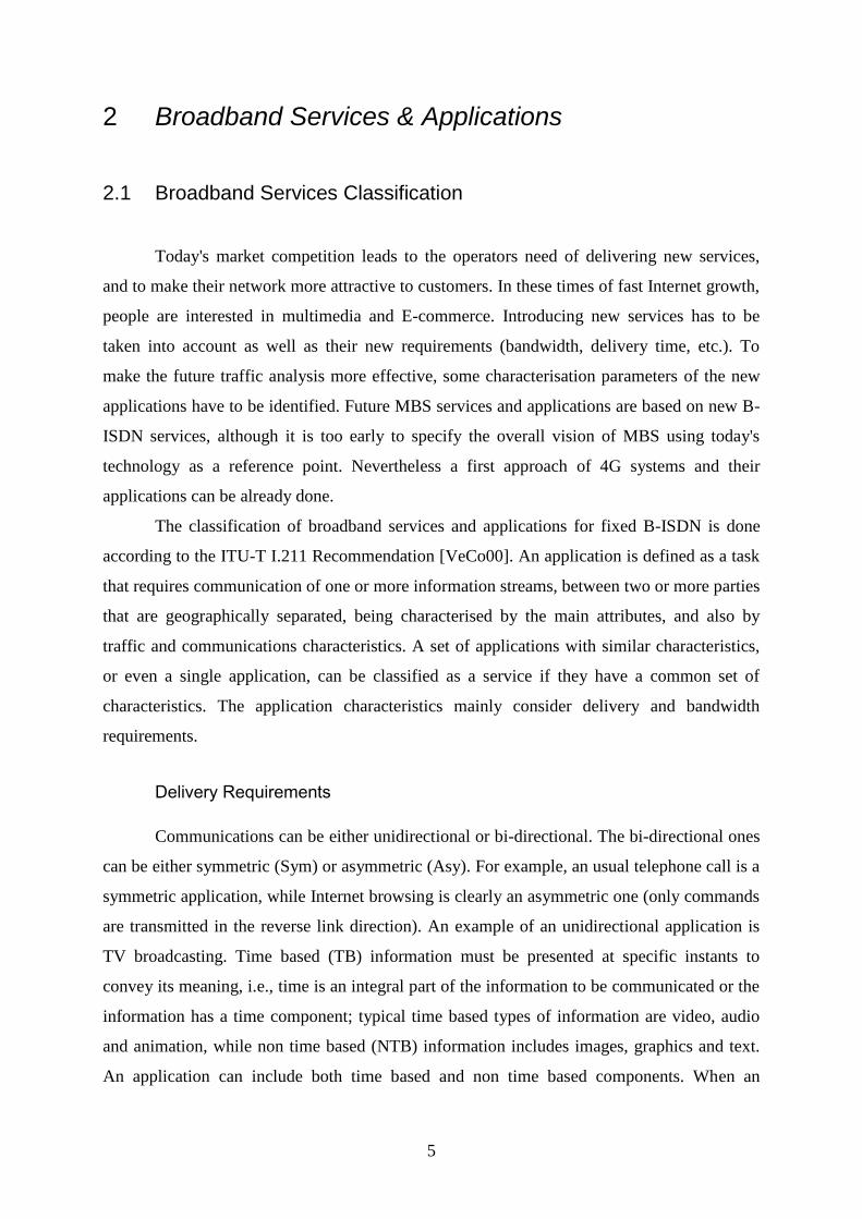
The future fourth generation Mobile Broadband System (MBS) concept is basically to
extend mobile users access to Broadband Integrated Services of Digital Networking (B-
ISDN) that will exist in future fixed networks, Figure 1.1. Around ten years from now, MBS
will play an important role in the mobile telecommunications market, mainly in large city
centres and urban areas where the highest demand is foreseen, while 3G systems are dedicated
to provide service to anyone, anytime, anywhere. Fourth generation MBS is also assumed to

2
support several services used simultaneously by the same user with the maximal bit rate up to
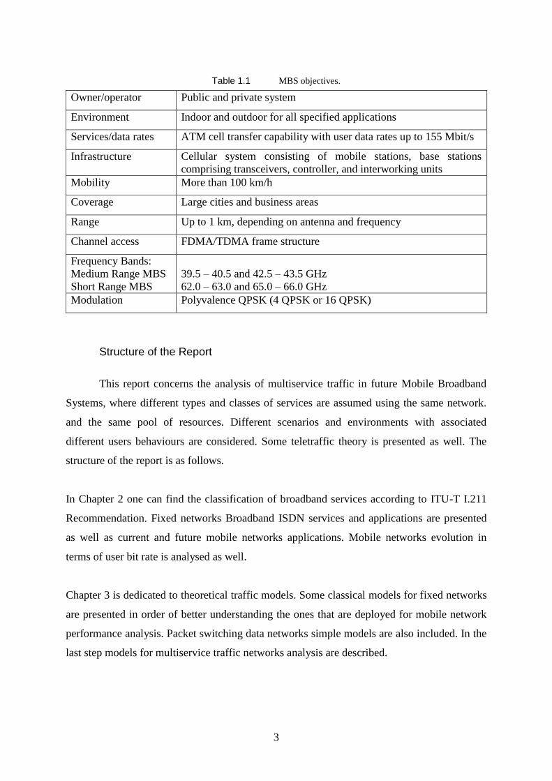
155 Mbit/s. Some today's assumptions for MBS are presented in Table 1.1.
Future applications must be considered differently in network planning and evolution
process from today's simple voice services. The GSM Association is expecting a high grade
of asymmetry between uplink and downlink for data based applications, with much higher
capacity needed for downlink. Due to the expected new system users behaviour while they are
using new services, teletraffic engineers should provide new models allowing communication
networks to be planned and systems to be designed more efficiently and economically, as well
as to meet a good performance. The Erlang B model for predicting blocking and Erlang C
model for predicting delay are still used extensively by teletraffic engineers in their daily
work while these formulas are not useful for multiservice modelling in Broadband networks.
New models have to be created and developed, which together with a deep understanding of
the technology and good applications characteristic can allow planning and dimensioning of
future network with all its phenomena.
Common Bacbone Network
DWDMA
240 x STM 64(240 x STM 128)
WorkstationFax
Telephone
Video
E3, VC 3
(25 - 30 Mbit/s)
Workstation
Workstation
Telephone
Small-Office
Home-Office
Workstation
Telephone Video
Interactiv e TV
E1 - E2, xDSL , VC12
2 - 8 Mbit/s
WorkstationWorkstation
Workstation
Workstation
Workstation
Workstation
Workstation
Workstation
Video
Video
Telephone
Telephone
Telephone
Telephone
Telephone
Fax
Fax
STM 1 - STM 4
B - ISDN
HOME
Office
BSS
BSS
BSS
MBS
STM 1 - STM 4
STM 4 - STM 64
(~53 Mbit/s by VDSL)
up to
155 Mbit/s
per user
Fiber optic
transmission path
Microwave
transmission path
Figure 1.1 Mobile Broadband System as extension to B-ISDN.
3
Table 1.1 MBS objectives.
Owner/operator Public and private system
Environment Indoor and outdoor for all specified applications
Services/data rates ATM cell transfer capability with user data rates up to 155 Mbit/s
Infrastructure Cellular system consisting of mobile stations, base stations
comprising transceivers, controller, and interworking units
Mobility More than 100 km/h
Coverage Large cities and business areas
Range Up to 1 km, depending on antenna and frequency
Channel access FDMA/TDMA frame structure
Frequency Bands:
Medium Range MBS
Short Range MBS
39.5 – 40.5 and 42.5 – 43.5 GHz
62.0 – 63.0 and 65.0 – 66.0 GHz
Modulation Polyvalence QPSK (4 QPSK or 16 QPSK)
Structure of the Report
This report concerns the analysis of multiservice traffic in future Mobile Broadband
Systems, where different types and classes of services are assumed using the same network.
and the same pool of resources. Different scenarios and environments with associated
different users behaviours are considered. Some teletraffic theory is presented as well. The
structure of the report is as follows.
In Chapter 2 one can find the classification of broadband services according to ITU-T I.211
Recommendation. Fixed networks Broadband ISDN services and applications are presented
as well as current and future mobile networks applications. Mobile networks evolution in
terms of user bit rate is analysed as well.
Chapter 3 is dedicated to theoretical traffic models. Some classical models for fixed networks
are presented in order of better understanding the ones that are deployed for mobile network
performance analysis. Packet switching data networks simple models are also included. In the
last step models for multiservice traffic networks analysis are described.

4
In Chapter 4 the Mobile Broadband System's approach is done in terms of future applications.
User's behaviour while using future applications in different environments is extensively
analysed and some performance evaluations are presented to the reader. Different duplexing
solutions (TDD or FDD) and their advantages and weakness are discussed of this chapter as
well.
Chapter 5 provides the reader with the main conclusions achieved during this work. Some
proposals for further research are also included.
5
2 Broadband Services & Applications
2.1 Broadband Services Classification
Today's market competition leads to the operators need of delivering new services,
and to make their network more attractive to customers. In these times of fast Internet growth,
people are interested in multimedia and E-commerce. Introducing new services has to be
taken into account as well as their new requirements (bandwidth, delivery time, etc.). To
make the future traffic analysis more effective, some characterisation parameters of the new
applications have to be identified. Future MBS services and applications are based on new B-
ISDN services, although it is too early to specify the overall vision of MBS using today's
technology as a reference point. Nevertheless a first approach of 4G systems and their
applications can be already done.
The classification of broadband services and applications for fixed B-ISDN is done
according to the ITU-T I.211 Recommendation [VeCo00]. An application is defined as a task
that requires communication of one or more information streams, between two or more parties
that are geographically separated, being characterised by the main attributes, and also by
traffic and communications characteristics. A set of applications with similar characteristics,
or even a single application, can be classified as a service if they have a common set of
characteristics. The application characteristics mainly consider delivery and bandwidth
requirements.
Delivery Requirements
Communications can be either unidirectional or bi-directional. The bi-directional ones
can be either symmetric (Sym) or asymmetric (Asy). For example, an usual telephone call is a
symmetric application, while Internet browsing is clearly an asymmetric one (only commands
are transmitted in the reverse link direction). An example of an unidirectional application is
TV broadcasting. Time based (TB) information must be presented at specific instants to
convey its meaning, i.e., time is an integral part of the information to be communicated or the
information has a time component; typical time based types of information are video, audio
and animation, while non time based (NTB) information includes images, graphics and text.
An application can include both time based and non time based components. When an
6
application involves multiple streams of information, synchronisation among them is an
important issue [Kwok95].
Regarding to delivery requirements an application can be defined either as real time
(RT) or a non real time (NRT) one. A real time application is one that requires information
delivery for immediate consumption, in contrast to non real time applications, in which
information can be stored temporarily at the receiving points (their buffers) for later
consumption. For example, a telephone conversation is considered a real-time application,
while sending electronic mail is a non real-time one [Kwok95]. In other words, users that
communicate via a real-time application must be present at the same time. Classes of delivery
are presented in Table 2.1.
Table 2.1 Example of applications with different information types and delivery requirements (extracted
from [Kwok95]).
Real Time Delivery Non Real Time Delivery
Time Based Information Video conferencing,
telephony
Video clip transfer
Non Time Based Information Image browsing Electronic mail
The bandwidth requirements of an application (in each direction) are typically
specified in terms of peak and average bandwidth. For Constant Bit Rate applications, the
peak and average bandwidths are the same [Kwok95]. Special mechanisms and protocols are
dedicated to protect delivery, bandwidth and quality requirements called Quality of Service
Controls.
Quality of Service Control
Quality of Service (QoS) generally can be described as a parameter responsible for
customer satisfaction. Traditional services are characterised on a point-to-point connection
basis by giving fixed limits for network performance parameters such the bit rate, bit error
rate (packet error rate), delay and jitters. Traditional networks have been Circuit Switched
with fixed capacity and deterministic delay or Packet Switched with Variable Bit Rate and
unpredictable delay by storing data in buffers. QoS parameter for these networks, like
maximum allowable bit error rate and delay time, are controlled by continuous measuring.
New services, in particular multimedia and broadband ones, require variable bandwidth and
techniques like point-to-multipoint connections. Communication requirements for such
services have to be defined by a sophisticated QoS framework, which has to be included in
future network's architecture bearing in mind the following aspects:
7
- full end to end connection;
- service quality requirements can change in time, even during session.
Therefore a QoS parameter control framework has to include:
- end to end QoS negotiation as set up time (admission control);
- policing to ensure that users are not violating negotiated QoS parameter (user
parameter control);
- monitoring to ensure that negotiated QoS levels are being maintained by the service
provider.
Classification
The description of B-ISDN services and applications is organised according to ITU-T
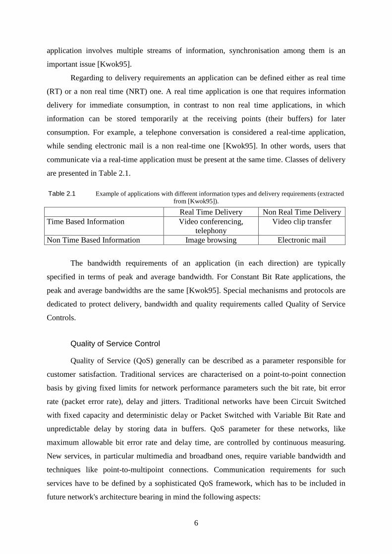
I.211 Recommendation. The work of [VeCo00] is used in what follows. Basic components
are: audio, video and data, Figure 2.1.
Serv ice commponents
Audio
Data
Video
Voice
HI-FI
Medium Rate (MED)
Low Rate (LOD)
High Def init ion Video
Interactiv e Video
High Rate (HID)
Figure 2.1 Basic service components (extracted from [VeCo00]).
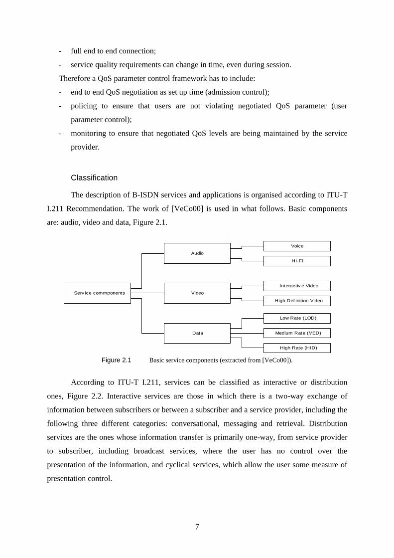
According to ITU-T I.211, services can be classified as interactive or distribution
ones, Figure 2.2. Interactive services are those in which there is a two-way exchange of
information between subscribers or between a subscriber and a service provider, including the
following three different categories: conversational, messaging and retrieval. Distribution
services are the ones whose information transfer is primarily one-way, from service provider
to subscriber, including broadcast services, where the user has no control over the
presentation of the information, and cyclical services, which allow the user some measure of
presentation control.
8
Interactiv e Serv ices
Distribution Serv ices
Conv ersational Messaging Retriev al
Broadcast Cy clical
Figure 2.2 Classification of services according to ITU-T I.211 (extracted from [VeCo00]).
Conversational Services provide the means for bi-directional dialogue communication
with bi-directional, real-time (not store and forward), end-to-end information transfer between
two users, or between a user and a service provider host. The flow of information may be bi-
directional symmetric or bi-directional asymmetric, and in some specific cases (e.g., video
surveillance) the flow of information may be unidirectional.
Messaging Services offer user-to-user communication between individual users via
storage units with store and forward, mailbox, and/or message-handling (e.g., information
editing, processing and conversion) functions. In contrast to conversational services,
messaging services are non real-time. Hence, they place lesser demands on the network and
do not require that both users be available at the same time.
Retrieval Services provide the user with the capability to retrieve information stored in
information centres that is, in general, available for public use. This information is sent to the
user on demand only, with the possibility of being retrieved on an individual basis, i.e., the
time at which an information sequence is started is under the control of the user. Examples are
broadband retrieval services for film, high resolution image, audio information and archival
information. An analogous narrowband service is videotext.
Broadcast Services provide a continuous flow of information, which is distributed
from a central source to an unlimited number of authorised retrievers connected to the
network. Each user can access this flow of information, but has no control over it; in
particular, the user cannot control the starting time or order the presentation of the
broadcasted information. All users simply tap into the flow of information. Depending on the
instant of time the user accesses as the information may not be presented from the beginning.
9
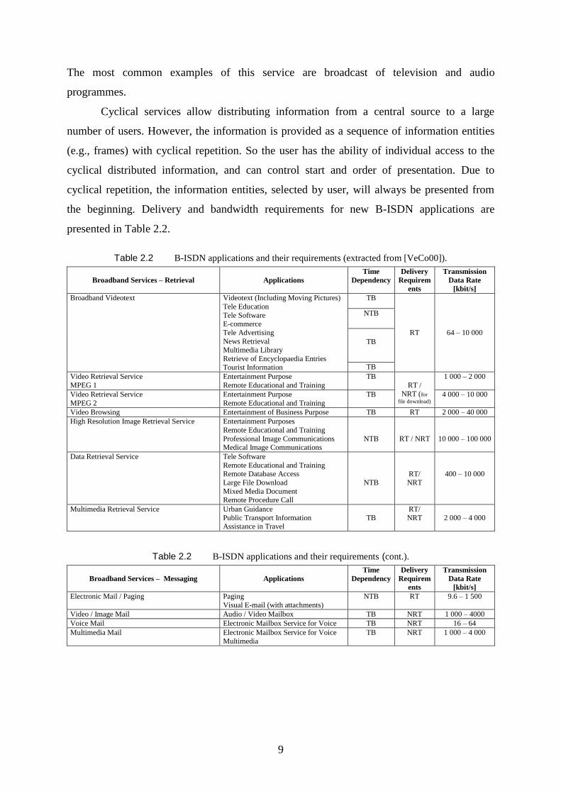
The most common examples of this service are broadcast of television and audio
programmes.
Cyclical services allow distributing information from a central source to a large
number of users. However, the information is provided as a sequence of information entities
(e.g., frames) with cyclical repetition. So the user has the ability of individual access to the
cyclical distributed information, and can control start and order of presentation. Due to
cyclical repetition, the information entities, selected by user, will always be presented from
the beginning. Delivery and bandwidth requirements for new B-ISDN applications are
presented in Table 2.2.
Table 2.2 B-ISDN applications and their requirements (extracted from [VeCo00]).
Broadband Services – Retrieval
Applications
Time
Dependency
Delivery
Requirem
ents
Transmission
Data Rate
[kbit/s]
Broadband Videotext Videotext (Including Moving Pictures)
Tele Education
Tele Software E-commerce
Tele Advertising
News Retrieval Multimedia Library
Retrieve of Encyclopaedia Entries
Tourist Information
TB
RT
64 – 10 000
NTB
TB
TB
Video Retrieval Service
MPEG 1
Entertainment Purpose
Remote Educational and Training
TB
RT /
NRT (for
file download)
1 000 – 2 000
Video Retrieval Service
MPEG 2
Entertainment Purpose
Remote Educational and Training
TB 4 000 – 10 000
Video Browsing Entertainment of Business Purpose TB RT 2 000 – 40 000
High Resolution Image Retrieval Service Entertainment Purposes
Remote Educational and Training
Professional Image Communications Medical Image Communications
NTB
RT / NRT
10 000 – 100 000
Data Retrieval Service Tele Software
Remote Educational and Training Remote Database Access
Large File Download
Mixed Media Document Remote Procedure Call
NTB
RT/
NRT
400 – 10 000
Multimedia Retrieval Service Urban Guidance
Public Transport Information Assistance in Travel
TB
RT/
NRT
2 000 – 4 000
Table 2.2 B-ISDN applications and their requirements (cont.).
Broadband Services – Messaging
Applications
Time
Dependency
Delivery
Requirem
ents
Transmission
Data Rate
[kbit/s]
Electronic Mail / Paging Paging
Visual E-mail (with attachments)
NTB RT 9.6 – 1 500
Video / Image Mail Audio / Video Mailbox TB NRT 1 000 – 4000
Voice Mail Electronic Mailbox Service for Voice TB NRT 16 – 64
Multimedia Mail Electronic Mailbox Service for Voice
Multimedia
TB NRT 1 000 – 4 000
10
Table 2.2 B-ISDN applications and their requirements (cont.).
Broadband Services – Conversational
Applications
Time
Dependency
Delivery
Requirem
ents
Transmission
Data Rate
[kbit/s]
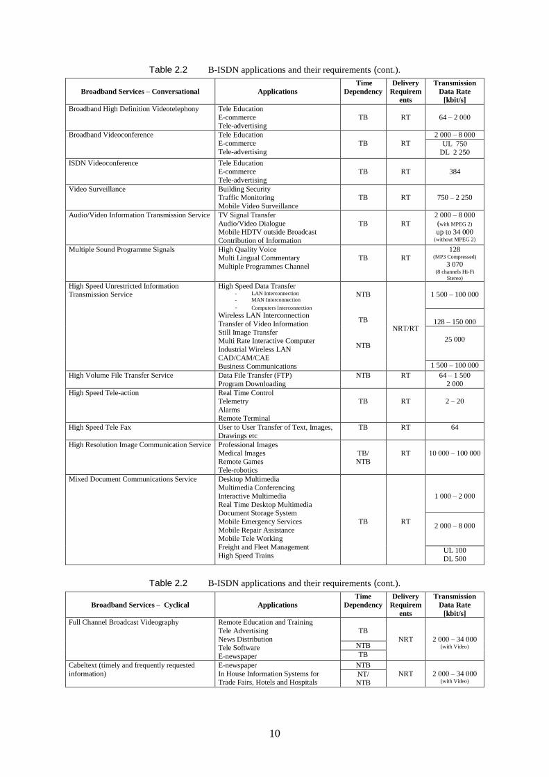
Broadband High Definition Videotelephony Tele Education
E-commerce Tele-advertising
TB
RT
64 – 2 000
Broadband Videoconference Tele Education
E-commerce
Tele-advertising
TB
RT
2 000 – 8 000
UL 750
DL 2 250
ISDN Videoconference Tele Education E-commerce
Tele-advertising
TB
RT
384
Video Surveillance Building Security Traffic Monitoring
Mobile Video Surveillance
TB
RT
750 – 2 250
Audio/Video Information Transmission Service TV Signal Transfer
Audio/Video Dialogue Mobile HDTV outside Broadcast
Contribution of Information
TB
RT
2 000 – 8 000
(with MPEG 2)
up to 34 000
(without MPEG 2)
Multiple Sound Programme Signals High Quality Voice Multi Lingual Commentary
Multiple Programmes Channel
TB
RT
128 (MP3 Compressed)
3 070 (8 channels Hi-Fi
Stereo)
High Speed Unrestricted Information Transmission Service
High Speed Data Transfer - LAN Interconnection
- MAN Interconnection
- Computers Interconnection Wireless LAN Interconnection
Transfer of Video Information
Still Image Transfer Multi Rate Interactive Computer
Industrial Wireless LAN
CAD/CAM/CAE Business Communications
NTB
TB
NTB
NRT/RT
1 500 – 100 000
128 – 150 000
25 000
1 500 – 100 000
High Volume File Transfer Service Data File Transfer (FTP)
Program Downloading
NTB RT 64 – 1 500
2 000
High Speed Tele-action Real Time Control Telemetry
Alarms
Remote Terminal
TB
RT
2 – 20
High Speed Tele Fax User to User Transfer of Text, Images, Drawings etc
TB RT 64
High Resolution Image Communication Service Professional Images
Medical Images Remote Games
Tele-robotics
TB/ NTB
RT
10 000 – 100 000
Mixed Document Communications Service Desktop Multimedia Multimedia Conferencing
Interactive Multimedia
Real Time Desktop Multimedia Document Storage System
Mobile Emergency Services
Mobile Repair Assistance Mobile Tele Working
Freight and Fleet Management
High Speed Trains
TB
RT
1 000 – 2 000
2 000 – 8 000
UL 100
DL 500
Table 2.2 B-ISDN applications and their requirements (cont.).
Broadband Services – Cyclical
Applications
Time
Dependency
Delivery
Requirem
ents
Transmission
Data Rate
[kbit/s]
Full Channel Broadcast Videography Remote Education and Training
Tele Advertising
News Distribution Tele Software
E-newspaper
TB
NRT
2 000 – 34 000 (with Video) NTB
TB
Cabeltext (timely and frequently requested
information)
E-newspaper
In House Information Systems for
Trade Fairs, Hotels and Hospitals
NTB
NRT
2 000 – 34 000 (with Video)
NT/
NTB
11
Table 2.2 B-ISDN applications and their requirements (cont.).
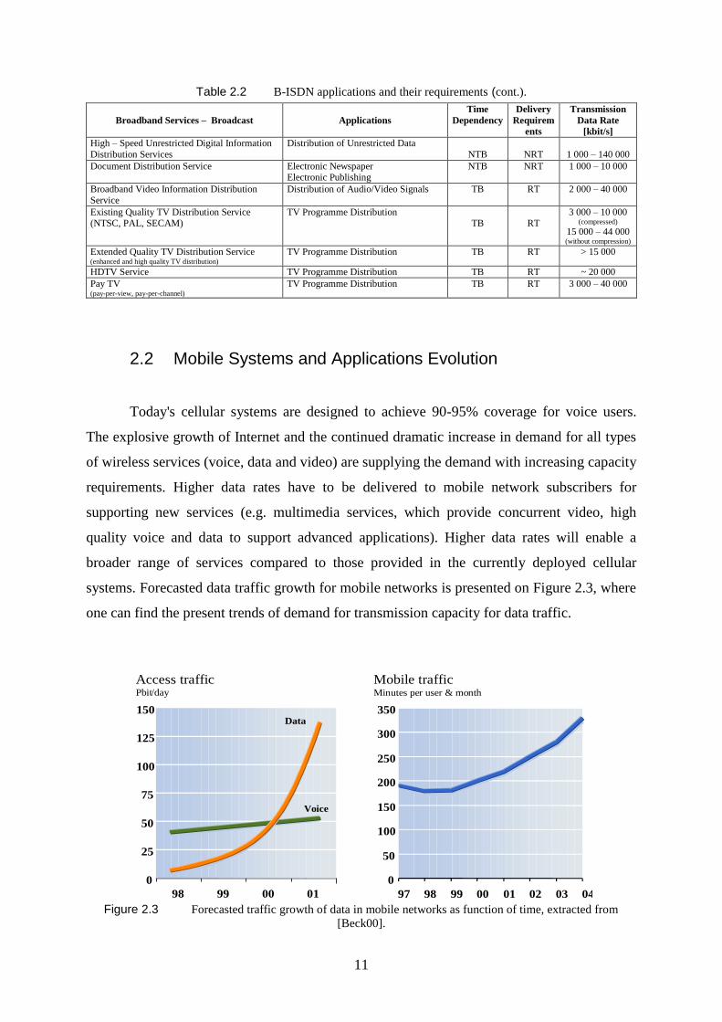
Broadband Services – Broadcast
Applications
Time
Dependency
Delivery
Requirem
ents
Transmission
Data Rate
[kbit/s]
High – Speed Unrestricted Digital Information
Distribution Services
Distribution of Unrestricted Data
NTB
NRT
1 000 – 140 000
Document Distribution Service Electronic Newspaper Electronic Publishing
NTB NRT 1 000 – 10 000
Broadband Video Information Distribution
Service
Distribution of Audio/Video Signals TB RT 2 000 – 40 000
Existing Quality TV Distribution Service (NTSC, PAL, SECAM)
TV Programme Distribution TB
RT
3 000 – 10 000 (compressed)
15 000 – 44 000 (without compression)
Extended Quality TV Distribution Service (enhanced and high quality TV distribution)
TV Programme Distribution TB RT > 15 000
HDTV Service TV Programme Distribution TB RT ~ 20 000
Pay TV (pay-per-view, pay-per-channel)
TV Programme Distribution TB RT 3 000 – 40 000
2.2 Mobile Systems and Applications Evolution
Today's cellular systems are designed to achieve 90-95% coverage for voice users.
The explosive growth of Internet and the continued dramatic increase in demand for all types
of wireless services (voice, data and video) are supplying the demand with increasing capacity
requirements. Higher data rates have to be delivered to mobile network subscribers for
supporting new services (e.g. multimedia services, which provide concurrent video, high
quality voice and data to support advanced applications). Higher data rates will enable a
broader range of services compared to those provided in the currently deployed cellular
systems. Forecasted data traffic growth for mobile networks is presented on Figure 2.3, where
one can find the present trends of demand for transmission capacity for data traffic.
Mobile trafficMinutes per user & month
0
50
100
150
200
250
300
350
97 98 99 00 01 02 03 04
0
98 99 00 01
25
50
75
100
125
150
Access trafficPbit/day
Voice
Data
(Internet)
Figure 2.3 Forecasted traffic growth of data in mobile networks as function of time, extracted from
[Beck00].
12
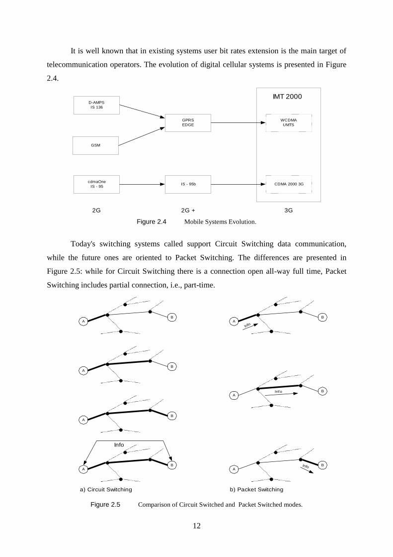
It is well known that in existing systems user bit rates extension is the main target of
telecommunication operators. The evolution of digital cellular systems is presented in Figure
2.4.
D-AMPS
IS 136
GSM
cdmaOne
IS - 95
GPRS
EDGE
IS - 95b CDMA 2000 3G
WCDMA
UMTS
IMT 2000
2G 3G2G +
Figure 2.4 Mobile Systems Evolution.
Today's switching systems called support Circuit Switching data communication,
while the future ones are oriented to Packet Switching. The differences are presented in
Figure 2.5: while for Circuit Switching there is a connection open all-way full time, Packet
Switching includes partial connection, i.e., part-time.
AB
a) Circuit Switching
AB
AB
AB
AB
AB
AB
Info
Info
Inf o
Info
b) Packet Switching
Figure 2.5 Comparison of Circuit Switched and Packet Switched modes.
13
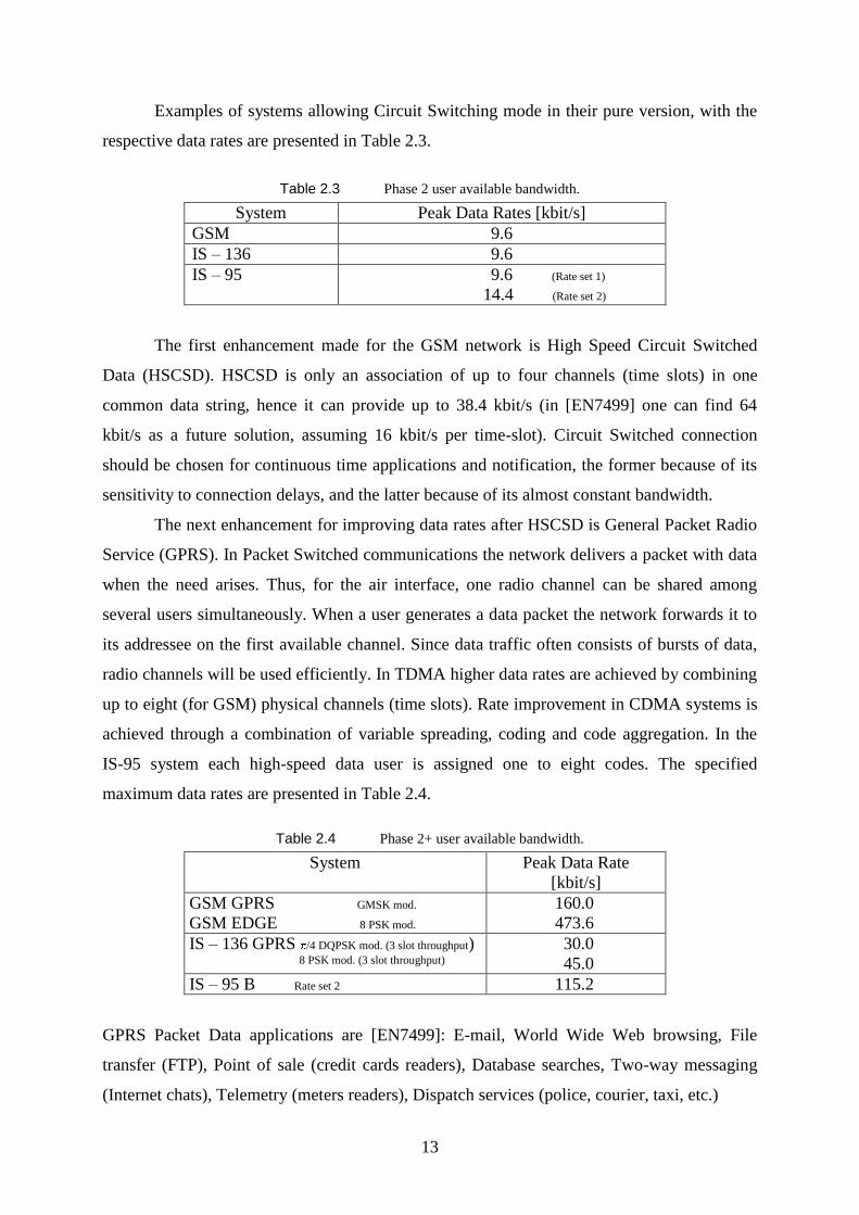
Examples of systems allowing Circuit Switching mode in their pure version, with the
respective data rates are presented in Table 2.3.
Table 2.3 Phase 2 user available bandwidth.
System Peak Data Rates [kbit/s]
GSM 9.6
IS – 136 9.6
IS – 95 9.6 (Rate set 1)
14.4 (Rate set 2)
The first enhancement made for the GSM network is High Speed Circuit Switched
Data (HSCSD). HSCSD is only an association of up to four channels (time slots) in one
common data string, hence it can provide up to 38.4 kbit/s (in [EN7499] one can find 64
kbit/s as a future solution, assuming 16 kbit/s per time-slot). Circuit Switched connection
should be chosen for continuous time applications and notification, the former because of its
sensitivity to connection delays, and the latter because of its almost constant bandwidth.
The next enhancement for improving data rates after HSCSD is General Packet Radio
Service (GPRS). In Packet Switched communications the network delivers a packet with data
when the need arises. Thus, for the air interface, one radio channel can be shared among
several users simultaneously. When a user generates a data packet the network forwards it to
its addressee on the first available channel. Since data traffic often consists of bursts of data,
radio channels will be used efficiently. In TDMA higher data rates are achieved by combining
up to eight (for GSM) physical channels (time slots). Rate improvement in CDMA systems is
achieved through a combination of variable spreading, coding and code aggregation. In the
IS-95 system each high-speed data user is assigned one to eight codes. The specified
maximum data rates are presented in Table 2.4.
Table 2.4 Phase 2+ user available bandwidth.
System Peak Data Rate
[kbit/s]
GSM GPRS GMSK mod.
GSM EDGE 8 PSK mod.
160.0
473.6
IS – 136 GPRS /4 DQPSK mod. (3 slot throughput) 8 PSK mod. (3 slot throughput)
30.0
45.0
IS – 95 B Rate set 2 115.2
GPRS Packet Data applications are [EN7499]: E-mail, World Wide Web browsing, File
transfer (FTP), Point of sale (credit cards readers), Database searches, Two-way messaging
(Internet chats), Telemetry (meters readers), Dispatch services (police, courier, taxi, etc.)
14
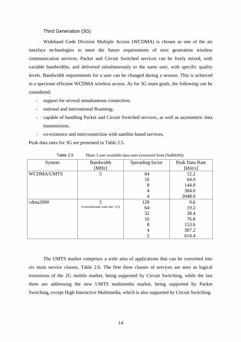
Third Generation (3G)
Wideband Code Division Multiple Access (WCDMA) is chosen as one of the air
interface technologies to meet the future requirements of next generation wireless
communication services. Packet and Circuit Switched services can be freely mixed, with
variable bandwidths, and delivered simultaneously to the same user, with specific quality
levels. Bandwidth requirements for a user can be changed during a session. This is achieved
in a spectrum efficient WCDMA wireless access. As for 3G main goals, the following can be
considered:
- support for several simultaneous connection;
- national and international Roaming;
- capable of handling Packet and Circuit Switched services, as well as asymmetric data
transmission;
- co-existence and interconnection with satellite based services.
Peak data rates for 3G are presented in Table 2.5.
Table 2.5 Phase 3 user available data rates (extracted from [NaBK00]).
System Bandwidth
[MHz]
Spreading factor Peak Data Rate
[kbit/s]
WCDMA/UMTS 5 64
16
8
4
4
12.2
64.0
144.0
384.0
2048.0
cdma2000 5 (convolutional code rate: 1/3)
128
64
32
16
8
4
2
9.6
19.2
38.4
76.8
153.6
307.2
614.4
The UMTS market comprises a wide area of applications that can be converted into
six main service classes, Table 2.6. The first three classes of services are seen as logical
extensions of the 2G mobile market, being supported by Circuit Switching, while the last
three are addressing the new UMTS multimedia market, being supported by Packet
Switching, except High Interactive Multimedia, which is also supported by Circuit Switching.
15
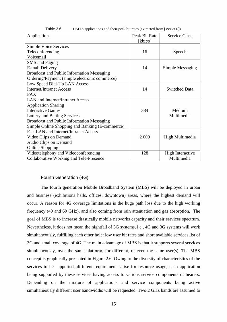
Table 2.6 UMTS applications and their peak bit rates (extracted from [VeCo00]).
Application Peak Bit Rate
[kbit/s]
Service Class
Simple Voice Services
Teleconferencing
Voicemail
16
Speech
SMS and Paging
E-mail Delivery
Broadcast and Public Information Messaging
Ordering/Payment (simple electronic commerce)
14
Simple Messaging
Low Speed Dial-Up LAN Access
Internet/Intranet Access
FAX
14
Switched Data
LAN and Internet/Intranet Access
Application Sharing
Interactive Games
Lottery and Betting Services
Broadcast and Public Information Messaging
Simple Online Shopping and Banking (E-commerce)
384
Medium
Multimedia
Fast LAN and Internet/Intranet Access
Video Clips on Demand
Audio Clips on Demand
Online Shopping
2 000
High Multimedia
Videotelephony and Videoconferencing
Collaborative Working and Tele-Presence
128 High Interactive
Multimedia
Fourth Generation (4G)
The fourth generation Mobile Broadband System (MBS) will be deployed in urban
and business (exhibitions halls, offices, downtown) areas, where the highest demand will
occur. A reason for 4G coverage limitations is the huge path loss due to the high working
frequency (40 and 60 GHz), and also coming from rain attenuation and gas absorption. The
goal of MBS is to increase drastically mobile networks capacity and their services spectrum.
Nevertheless, it does not mean the nightfall of 3G systems, i.e., 4G and 3G systems will work
simultaneously, fulfilling each other hole: low user bit rates and short available services list of
3G and small coverage of 4G. The main advantage of MBS is that it supports several services
simultaneously, over the same platform, for different, or even the same user(s). The MBS
concept is graphically presented in Figure 2.6. Owing to the diversity of characteristics of the
services to be supported, different requirements arise for resource usage, each application
being supported by these services having access to various service components or bearers.
Depending on the mixture of applications and service components being active
simultaneously different user bandwidths will be requested. Two 2 GHz bands are assumed to
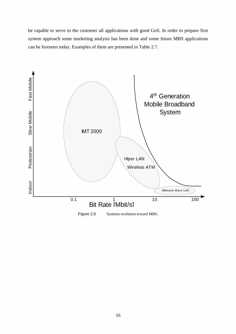
16
be capable to serve to the customer all applications with good GoS. In order to prepare first
system approach some marketing analysis has been done and some future MBS applications
can be foreseen today. Examples of them are presented in Table 2.7.
0.1 1 10010
Ind
oo
rP
ed
estr
ian
Slo
w M
ob
ileF
ast
Mo
bile
4th Generation
Mobile Broadband
System
Milimetre Wav e LAN
IMT 2000
Hiper LAN
Wireless ATM
Bit Rate [Mbit/s]
Figure 2.6 Systems evolution toward MBS.
17
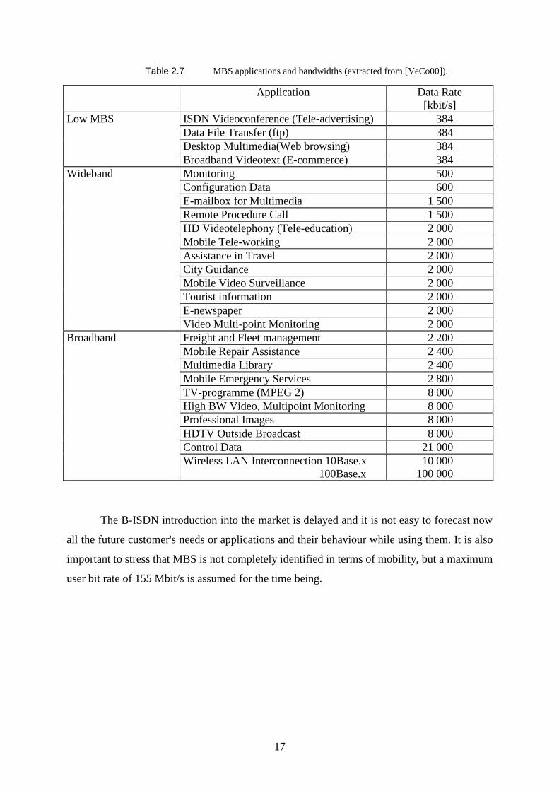
Table 2.7 MBS applications and bandwidths (extracted from [VeCo00]).
Application Data Rate
[kbit/s]
Low MBS ISDN Videoconference (Tele-advertising) 384
Data File Transfer (ftp) 384
Desktop Multimedia(Web browsing) 384
Broadband Videotext (E-commerce) 384
Wideband Monitoring 500
Configuration Data 600
E-mailbox for Multimedia 1 500
Remote Procedure Call 1 500
HD Videotelephony (Tele-education) 2 000
Mobile Tele-working 2 000
Assistance in Travel 2 000
City Guidance 2 000
Mobile Video Surveillance 2 000
Tourist information 2 000
E-newspaper 2 000
Video Multi-point Monitoring 2 000
Broadband Freight and Fleet management 2 200
Mobile Repair Assistance 2 400
Multimedia Library 2 400
Mobile Emergency Services 2 800
TV-programme (MPEG 2) 8 000
High BW Video, Multipoint Monitoring 8 000
Professional Images 8 000
HDTV Outside Broadcast 8 000
Control Data 21 000
Wireless LAN Interconnection 10Base.x
100Base.x
10 000
100 000
The B-ISDN introduction into the market is delayed and it is not easy to forecast now
all the future customer's needs or applications and their behaviour while using them. It is also
important to stress that MBS is not completely identified in terms of mobility, but a maximum
user bit rate of 155 Mbit/s is assumed for the time being.

18
19
3 Traffic theory basis
3.1 Introduction
Telecommunication systems use trunks to accommodate a large number of users in
limited transmission abilities. The concept of trunking allows a large number of users to share
the relatively small number of channels in a chosen area by providing each user access to
resources on demand, from a pool of available channels. Trunking exploits the statistical
behaviour of users and calls so that a fixed number of channels may accommodate a large,
random user community. Probability theory is used to calculate the requirements for resources
and their utilisation.
3.2 Intensity and Units of Traffic
Traffic intensity is measured in Erlang, the name of the Danish mathematician, who
found telephone traffic theory. Using the Erlang formula, the calculation of traffic generated
by one user can be defined as follows [Yaco93]:
Erlang u
uuA (3.1)
1-s 1
Tu (3.2)
where:
– Average number of calls generated by user per time unit
T – Average call holding time (average duration of call) generated by user
– Average service rate
Hence, typically it is represented as follows:
Erlang s 3600
s TAu (3.3)
From this, the total traffic in a chosen area is calculated by summing the traffic generated by
each system user in the considered area:

20
Erlang 0
u
u
N
u
AA (3.4)
where:
Nu – number of served users
Congestion time is the period of time during which all channels available in the
system are busy. Thus new incoming calls will be denied. In that case, the following relation
exists for the set of available channels:
cn = 1 Erlang (3.5)
where:
cn – maximal traffic from the independent channel n
Hence, the total traffic offered by one channel is less or equal to 1 Erlang.
3.3 Birth & Death Process
Let Sk denote the state of the system when the number of busy channels is k. In the
Markov chain model transitions are only allowed between neighbouring states, hence
transition from Sk to Sk+1 implies that a new channel will get busy with rate k, and transition
from Sk to Sk-1 implies channel releasing with rate k , Figure 3.1[Yaco93].
0 k+1kk-121
0 1 k-1 k
k+1k21
...
Figure 3.1 State transition diagram for one dimensional birth death process.
Let pk be the probability that the system is in state Sk at time t (k represents the number
of system channels being busy). Inspecting Figure 3.1, the probability of reaching state Sk can
be represented as:
Sk = [ k-1 pk-1 + k+1 pk+1] dt (3.6)
and the probability of departing from state Sk is given by:
Sk = ( k + k)dt pk (3.7)
By differentiation one obtains the equilibrium equation
21
0 1111 kppp kkkkkkk (3.8)
where:
p-1 = 0 (less then 0 channels cannot be allocated)
0 = 0
-1 = 0
Equation 3.8 shows that, in equilibrium, the rate of flow into the state Sk equals the
rate of flow out of Sk. By writing equation above sequentially, for k = 0,1,2,..., and observing
that the probabilities pk sum to unity, one obtains the following solution for the set of
equations:
1
0 10
k
i i
ik pp (3.9)
where:
1
1
1
0 110
k
k
i i
ip (3.10)
If one has a total of C channels in the system and considering i = i , where is the service
rate, pC corresponds to the Erlang B equation.
Grade of Service
The grade of service (GOS) is defined as the probability of call failure due to
transmission congestion and it is very often called Blocking Probability. Looking to the
Markov chain model, time congestion is the proportion of time when, for C available in
system channels, transitions terminate at state SC. All calls will fail if GOS = 1 and all calls
will pass if GOS = 0. Typical values are:
- 0.005 < GOS < 0.008 for fixed networks (depends on operator marketing demands);
- GOS = 0.02 for mobile networks.
3.4 Basic Aspects of Traffic Modelling
3.4.1 Bursty and Renewal Traffic
A recurrent theme relating to traffic in broadband networks is traffic burstiness
exhibited by key services such as compressed video, file transfer, etc., Figure 3.2. Burstiness
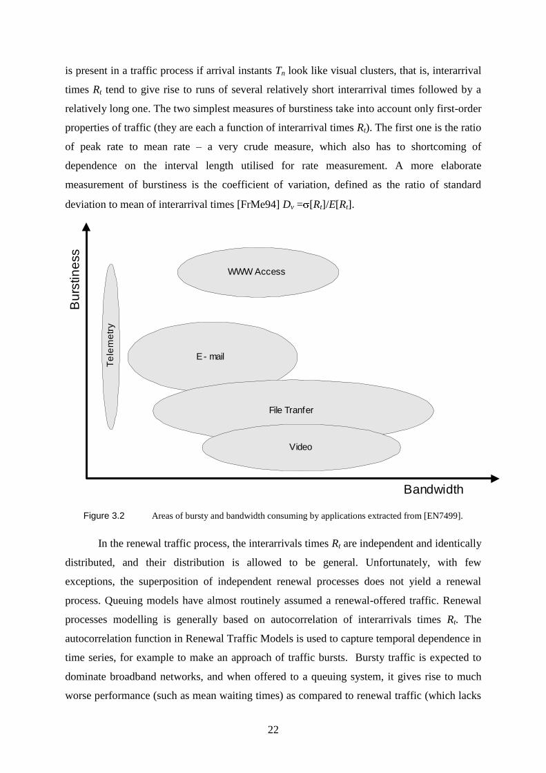
22
is present in a traffic process if arrival instants Tn look like visual clusters, that is, interarrival
times Rt tend to give rise to runs of several relatively short interarrival times followed by a
relatively long one. The two simplest measures of burstiness take into account only first-order
properties of traffic (they are each a function of interarrival times Rt). The first one is the ratio
of peak rate to mean rate – a very crude measure, which also has to shortcoming of
dependence on the interval length utilised for rate measurement. A more elaborate
measurement of burstiness is the coefficient of variation, defined as the ratio of standard
deviation to mean of interarrival times [FrMe94] Dv = [Rt]/E[Rt].
Bandwidth
Bu
rstin
ess
Te
lem
etr
y
E - mail
File Tranfer
Video
WWW Access
Figure 3.2 Areas of bursty and bandwidth consuming by applications extracted from [EN7499].
In the renewal traffic process, the interarrivals times Rt are independent and identically
distributed, and their distribution is allowed to be general. Unfortunately, with few
exceptions, the superposition of independent renewal processes does not yield a renewal
process. Queuing models have almost routinely assumed a renewal-offered traffic. Renewal
processes modelling is generally based on autocorrelation of interarrivals times Rt. The
autocorrelation function in Renewal Traffic Models is used to capture temporal dependence in
time series, for example to make an approach of traffic bursts. Bursty traffic is expected to
dominate broadband networks, and when offered to a queuing system, it gives rise to much
worse performance (such as mean waiting times) as compared to renewal traffic (which lacks
23
temporal dependence). Consequently, models that capture the autocorrelated nature of traffic
are essential for predicting the performance of emerging broadband networks.
3.4.2 Poisson Process
A Poisson process can be characterised as a renewal process whose interarrival times
Rt are exponentially distributed with rate parameter and probability Prob{Rt t}=1– exp(-
t). Poisson processes enjoy some elegant analytical properties. First, the superposition of
independent Poisson processes result in a new Poisson process whose rate is the sum of the
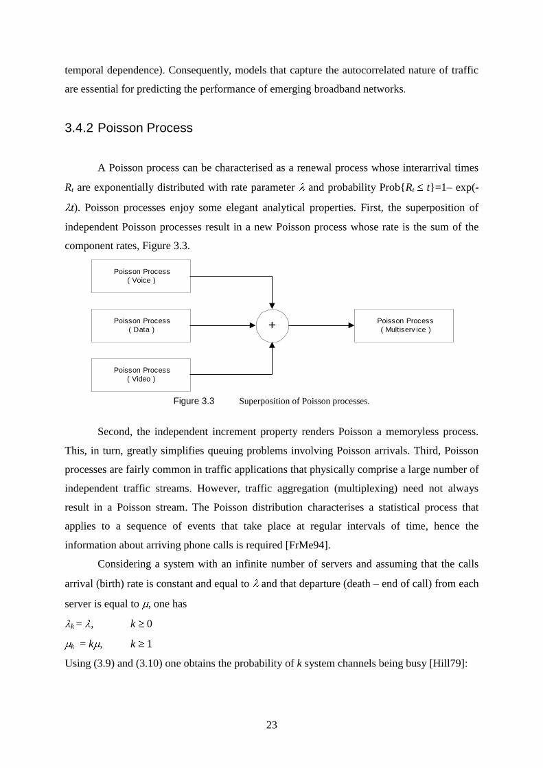
component rates, Figure 3.3.
Poisson Process
( Voice )
Poisson Process
( Data )
Poisson Process
( Video )
+ Poisson Process
( Multiserv ice )
Figure 3.3 Superposition of Poisson processes.
Second, the independent increment property renders Poisson a memoryless process.
This, in turn, greatly simplifies queuing problems involving Poisson arrivals. Third, Poisson
processes are fairly common in traffic applications that physically comprise a large number of
independent traffic streams. However, traffic aggregation (multiplexing) need not always
result in a Poisson stream. The Poisson distribution characterises a statistical process that
applies to a sequence of events that take place at regular intervals of time, hence the
information about arriving phone calls is required [FrMe94].
Considering a system with an infinite number of servers and assuming that the calls
arrival (birth) rate is constant and equal to and that departure (death – end of call) from each
server is equal to , one has
k = , k 0
k = k , k 1
Using (3.9) and (3.10) one obtains the probability of k system channels being busy [Hill79]:
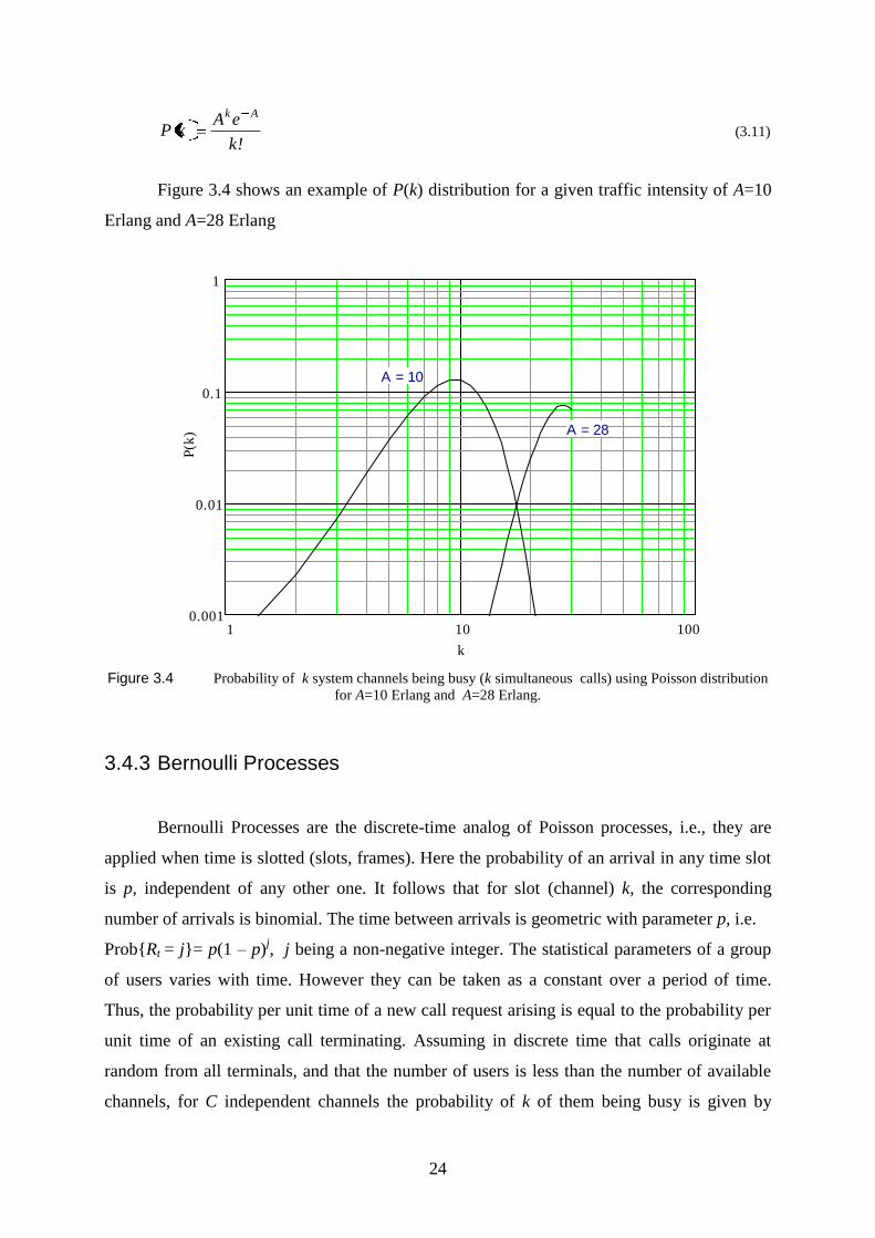
24
!k
eAkP
Ak
(3.11)
Figure 3.4 shows an example of P(k) distribution for a given traffic intensity of A=10
Erlang and A=28 Erlang
1 10 1000.001
0.01
0.1
1
k
P(k
)
A = 10
A = 28
Figure 3.4 Probability of k system channels being busy (k simultaneous calls) using Poisson distribution
for A=10 Erlang and A=28 Erlang.
3.4.3 Bernoulli Processes
Bernoulli Processes are the discrete-time analog of Poisson processes, i.e., they are
applied when time is slotted (slots, frames). Here the probability of an arrival in any time slot
is p, independent of any other one. It follows that for slot (channel) k, the corresponding
number of arrivals is binomial. The time between arrivals is geometric with parameter p, i.e.
Prob{Rt = j}= p(1 – p)j, j being a non-negative integer. The statistical parameters of a group
of users varies with time. However they can be taken as a constant over a period of time.
Thus, the probability per unit time of a new call request arising is equal to the probability per
unit time of an existing call terminating. Assuming in discrete time that calls originate at
random from all terminals, and that the number of users is less than the number of available
channels, for C independent channels the probability of k of them being busy is given by

25
Bernoulli distribution (because we cannot assume that P(k) is independent of the number of
calls being in progress) [Hill79]:
kuu
ku AA
kuk
ukP 1
!!
! (3.12)
where:
u – Number of system users (terminals)
k – Number of channels being busy
Typically the probability of k channels being busy is represented by curves as a function of
given traffic intensity A = Au u, Figure 3.5.
1 10 1000.001
0.01
0.1
1
k
P(k
)
u = 30
A = 28
A = 10
Figure 3.5 Probability of k system channels being busy (k simultaneous calls) using Bernoulli distribution
for A=10 Erlang and A=28 Erlang.
If a traffic of A Erlang arises from u users (terminals), when u the relation is transformed
into the Poisson distribution.
3.4.4 Markov and Markov-Renewal Traffic Models
Unlike renewal traffic models, Markov and Markov – Renewal traffic models
introduce dependence into the random sequence Rt. Consequently, they can potentially
capture traffic burstiness, because of nonzero autocorrelations in Rt. Consider a continuous-
time Markov process
26
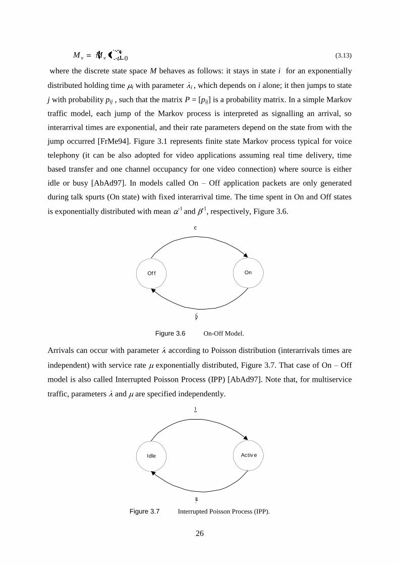
0ttMM vv (3.13)
where the discrete state space M behaves as follows: it stays in state i for an exponentially
distributed holding time i with parameter i , which depends on i alone; it then jumps to state
j with probability pij , such that the matrix P = [pij] is a probability matrix. In a simple Markov
traffic model, each jump of the Markov process is interpreted as signalling an arrival, so
interarrival times are exponential, and their rate parameters depend on the state from with the
jump occurred [FrMe94]. Figure 3.1 represents finite state Markov process typical for voice
telephony (it can be also adopted for video applications assuming real time delivery, time
based transfer and one channel occupancy for one video connection) where source is either
idle or busy [AbAd97]. In models called On – Off application packets are only generated
during talk spurts (On state) with fixed interarrival time. The time spent in On and Off states
is exponentially distributed with mean -1
and -1
, respectively, Figure 3.6.
Of f On
Figure 3.6 On-Off Model.
Arrivals can occur with parameter according to Poisson distribution (interarrivals times are
independent) with service rate exponentially distributed, Figure 3.7. That case of On – Off
model is also called Interrupted Poisson Process (IPP) [AbAd97]. Note that, for multiservice
traffic, parameters and are specified independently.
Idle Activ e
Figure 3.7 Interrupted Poisson Process (IPP).
27
Markov-Renewal models are more general than discrete-state Markov process, yet
retaining a measure of simplicity and analytical tractability. A Markov renewal process
0nnnr ,MM (3.14)
is defined by Markov a chain {Mn} and it is associated with jump times n, subject to the
following constraint: the pair (Mn+1, n+1) of the next state and inter-jump depends only on the
current state Mn , but not on previous states or on previous inter-jumps times [FrMe94]. This
means that all transitions are to the states just above (a birth) or to the state just below (a
death) and it is also quoted on Figure 3.1 as graph representing limited sources (channels)
telephony system. As it was assumed above, the Markov models can potentially capture
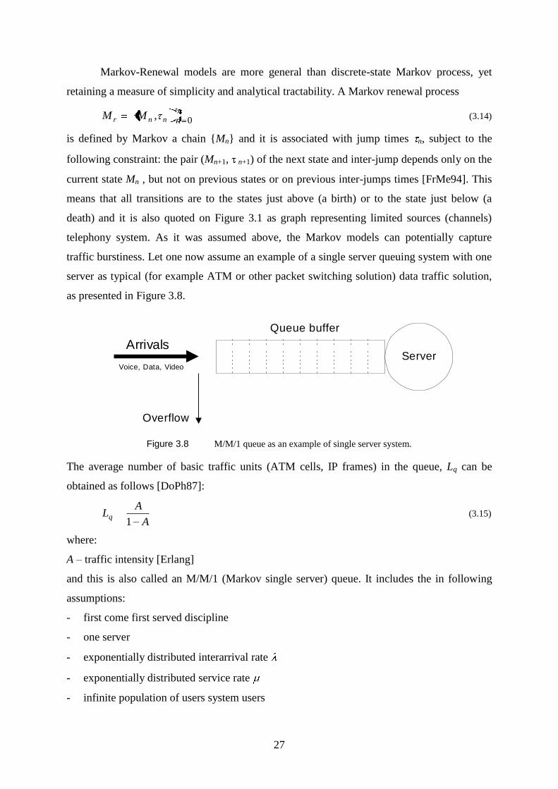
traffic burstiness. Let one now assume an example of a single server queuing system with one
server as typical (for example ATM or other packet switching solution) data traffic solution,
as presented in Figure 3.8.
Server
Queue buffer
Arrivals
Overflow
Voice, Data, Video
Figure 3.8 M/M/1 queue as an example of single server system.
The average number of basic traffic units (ATM cells, IP frames) in the queue, Lq can be
obtained as follows [DoPh87]:
A
ALq
1 (3.15)
where:
A – traffic intensity [Erlang]
and this is also called an M/M/1 (Markov single server) queue. It includes the in following
assumptions:
- first come first served discipline
- one server
- exponentially distributed interarrival rate
- exponentially distributed service rate
- infinite population of users system users
28
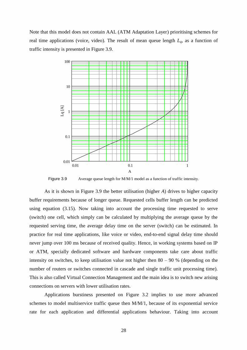
Note that this model does not contain AAL (ATM Adaptation Layer) prioritising schemes for
real time applications (voice, video). The result of mean queue length Lq, as a function of
traffic intensity is presented in Figure 3.9.
0.01 0.1 10.01
0.1
1
10
100
A
Lq
[A
]
Figure 3.9 Average queue length for M/M/1 model as a function of traffic intensity.
As it is shown in Figure 3.9 the better utilisation (higher A) drives to higher capacity
buffer requirements because of longer queue. Requested cells buffer length can be predicted
using equation (3.15). Now taking into account the processing time requested to serve
(switch) one cell, which simply can be calculated by multiplying the average queue by the
requested serving time, the average delay time on the server (switch) can be estimated. In
practice for real time applications, like voice or video, end-to-end signal delay time should
never jump over 100 ms because of received quality. Hence, in working systems based on IP
or ATM, specially dedicated software and hardware components take care about traffic
intensity on switches, to keep utilisation value not higher then 80 – 90 % (depending on the
number of routers or switches connected in cascade and single traffic unit processing time).
This is also called Virtual Connection Management and the main idea is to switch new arising
connections on servers with lower utilisation rates.
Applications burstiness presented on Figure 3.2 implies to use more advanced
schemes to model multiservice traffic queue then M/M/1, because of its exponential service
rate for each application and differential applications behaviour. Taking into account
29
differential service rate (time) and its variance for each application the M/G/1 model can be
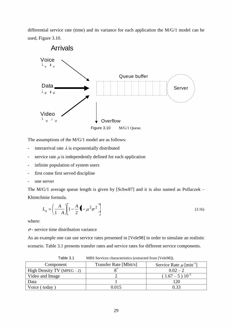
used, Figure 3.10.
Server
Queue buffer
Arrivals
Overflow
Voice
Video
Data
v
d
V
v
d
V
Figure 3.10 M/G/1 Queue.
The assumptions of the M/G/1 model are as follows:
- interarrival rate is exponentially distributed
- service rate is independently defined for each application
- infinite population of system users
- first come first served discipline
- one server
The M/G/1 average queue length is given by [Schw87] and it is also named as Pollaczek –
Khintchinie formula.
2212
11
A
A
ALq (3.16)
where:
- service time distribution variance
As an example one can use service rates presented in [Vele98] in order to simulate an realistic
scenario. Table 3.1 presents transfer rates and service rates for different service components.
Table 3.1 MBS Services characteristics (extracted from [Vele98]).
Component Transfer Rate [Mbit/s] Service Rate [min-1
]
High Density TV (MPEG – 2) 8* 0.02 – 2
Video and Image 2 ( 1.67 – 5 ) 10-3
Data 1 120
Voice ( today ) 0.015 0.33
30
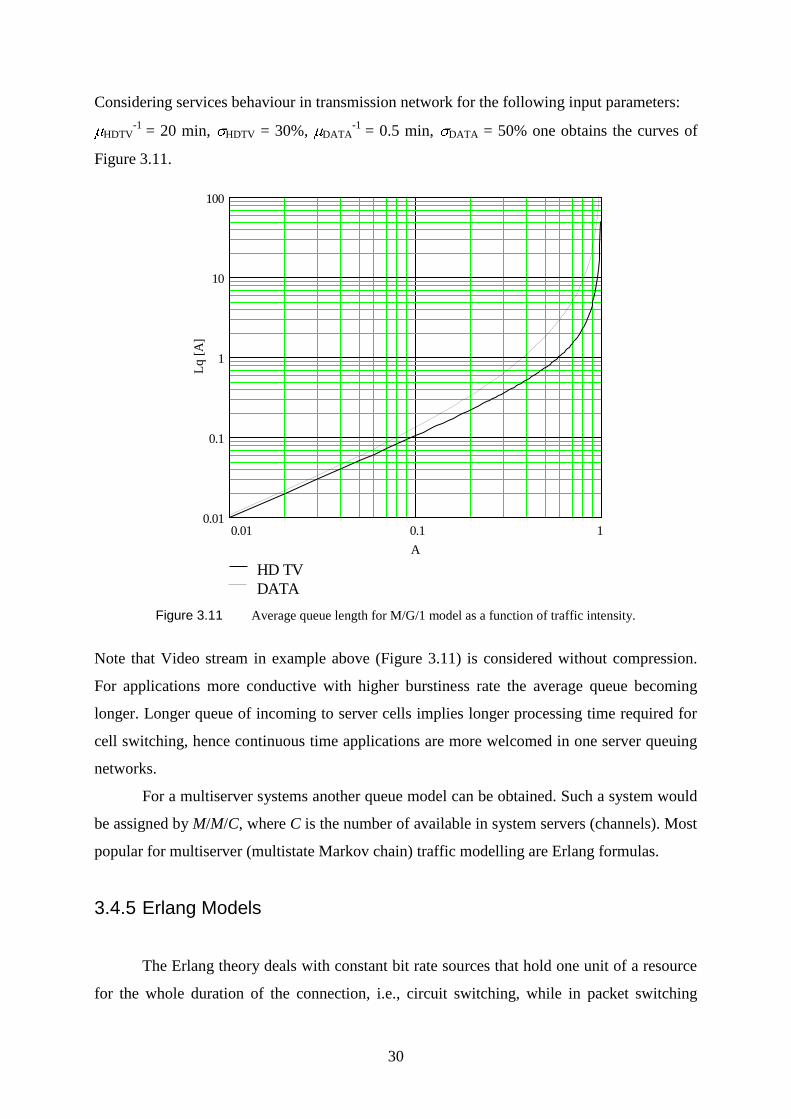
Considering services behaviour in transmission network for the following input parameters:
HDTV-1
= 20 min, HDTV = 30%, DATA-1
= 0.5 min, DATA = 50% one obtains the curves of
Figure 3.11.
0.01 0.1 10.01
0.1
1
10
100
HD TV
DATA
A
Lq
[A
]
Figure 3.11 Average queue length for M/G/1 model as a function of traffic intensity.
Note that Video stream in example above (Figure 3.11) is considered without compression.
For applications more conductive with higher burstiness rate the average queue becoming
longer. Longer queue of incoming to server cells implies longer processing time required for
cell switching, hence continuous time applications are more welcomed in one server queuing
networks.
For a multiserver systems another queue model can be obtained. Such a system would
be assigned by M/M/C, where C is the number of available in system servers (channels). Most
popular for multiserver (multistate Markov chain) traffic modelling are Erlang formulas.
3.4.5 Erlang Models
The Erlang theory deals with constant bit rate sources that hold one unit of a resource
for the whole duration of the connection, i.e., circuit switching, while in packet switching
31
networks (usually they are single server networks), traffic is segmented into blocks of data
(cells). The Erlang B model is useful for the systems where:
- the number of users is much greater than the number of available channels, such that no
matter how many devices are currently busy, the rate of call arrivals will be constant;
- if no channels are available, the requesting user is blocked without access and is free to try
again later (such system is also known as Blocked Calls Cleared);
- all users, including blocked ones, may request a channel;
- the probability of a user occupying a channel is exponentially determined;
- there are finite number of channels available in pool and all of them are accessible for
each user.
Blocked calls cleared this is the case of a Markov chain, when for C channels available in the
system transitions terminates at state SC and:
k = , k C - 1
k = k , k < C
Using equations (3.12) and (3.13) and for C available in system channels the blocking
probability (GOS) can be calculated by well known Erlang B formula as follows [Rapp96]:
GOS
k
A
C
A
PC
k
k
C
b
0 !
! (3.17)
The blocking probability arising from the traffic intensity A is usually represented as a
function of the number of available channels (given for each curve) C. The numbers of C=30
and C=100 are considered, Figure 3.12. A value of C=30 channels is typical for PDH E-1
(Plesiochronous Digital Hierarchy) level trunk and also approximately (depends on number
of dedicated signalling channels) to the number of physical channels in one cell of a GSM
network in an urban area. A value of C=100 channels is predicted value for future networks
(for example UMTS).
32
10 100 10000.001
0.01
0.1
1
A [Erlang]
GO
S [
%]
C = 30 C = 100
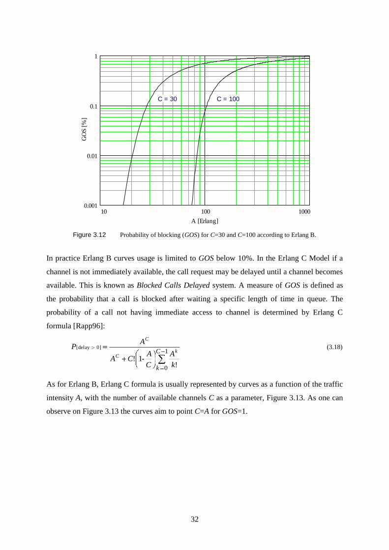
Figure 3.12 Probability of blocking (GOS) for C=30 and C=100 according to Erlang B.
In practice Erlang B curves usage is limited to GOS below 10%. In the Erlang C Model if a
channel is not immediately available, the call request may be delayed until a channel becomes
available. This is known as Blocked Calls Delayed system. A measure of GOS is defined as
the probability that a call is blocked after waiting a specific length of time in queue. The
probability of a call not having immediate access to channel is determined by Erlang C
formula [Rapp96]:
1
0 !1!
0]elayd[C
k k
A
C
A-CA
AP
kC
C
(3.18)
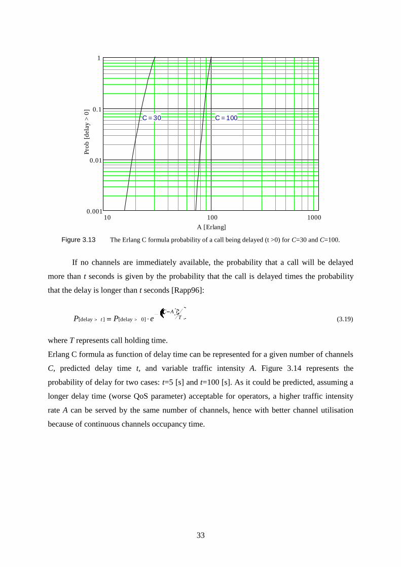
As for Erlang B, Erlang C formula is usually represented by curves as a function of the traffic
intensity A, with the number of available channels C as a parameter, Figure 3.13. As one can
observe on Figure 3.13 the curves aim to point C=A for GOS=1.
33
10 100 10000.001
0.01
0.1
1
A [Erlang]
Pro
b [
dela
y >
0]
C = 30 C = 100
Figure 3.13 The Erlang C formula probability of a call being delayed (t >0) for C=30 and C=100.
If no channels are immediately available, the probability that a call will be delayed
more than t seconds is given by the probability that the call is delayed times the probability
that the delay is longer than t seconds [Rapp96]:
TtAC
t ePP ]0[delay][delay (3.19)
where T represents call holding time.
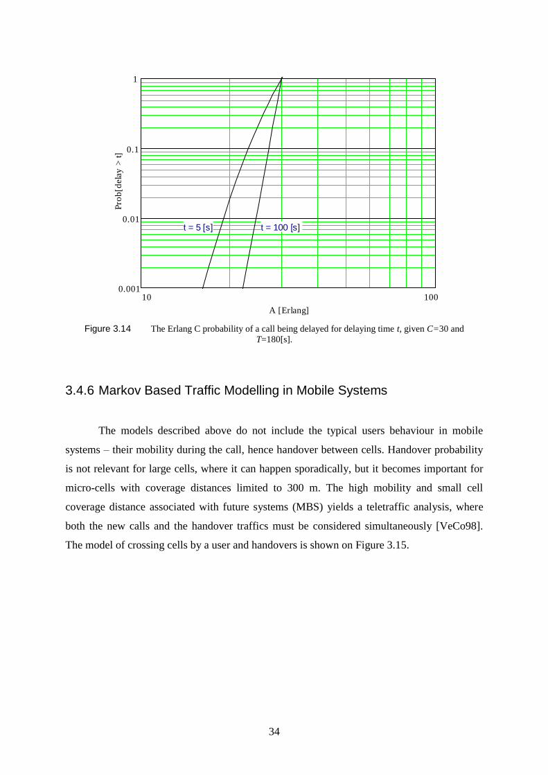
Erlang C formula as function of delay time can be represented for a given number of channels
C, predicted delay time t, and variable traffic intensity A. Figure 3.14 represents the
probability of delay for two cases: t=5 [s] and t=100 [s]. As it could be predicted, assuming a
longer delay time (worse QoS parameter) acceptable for operators, a higher traffic intensity
rate A can be served by the same number of channels, hence with better channel utilisation
because of continuous channels occupancy time.
34
10 1000.001
0.01
0.1
1
A [Erlang]
Pro
b[d
ela
y >
t]
t = 5 [s] t = 100 [s]
Figure 3.14 The Erlang C probability of a call being delayed for delaying time t, given C=30 and
T=180[s].
3.4.6 Markov Based Traffic Modelling in Mobile Systems
The models described above do not include the typical users behaviour in mobile
systems – their mobility during the call, hence handover between cells. Handover probability
is not relevant for large cells, where it can happen sporadically, but it becomes important for
micro-cells with coverage distances limited to 300 m. The high mobility and small cell
coverage distance associated with future systems (MBS) yields a teletraffic analysis, where
both the new calls and the handover traffics must be considered simultaneously [VeCo98].
The model of crossing cells by a user and handovers is shown on Figure 3.15.
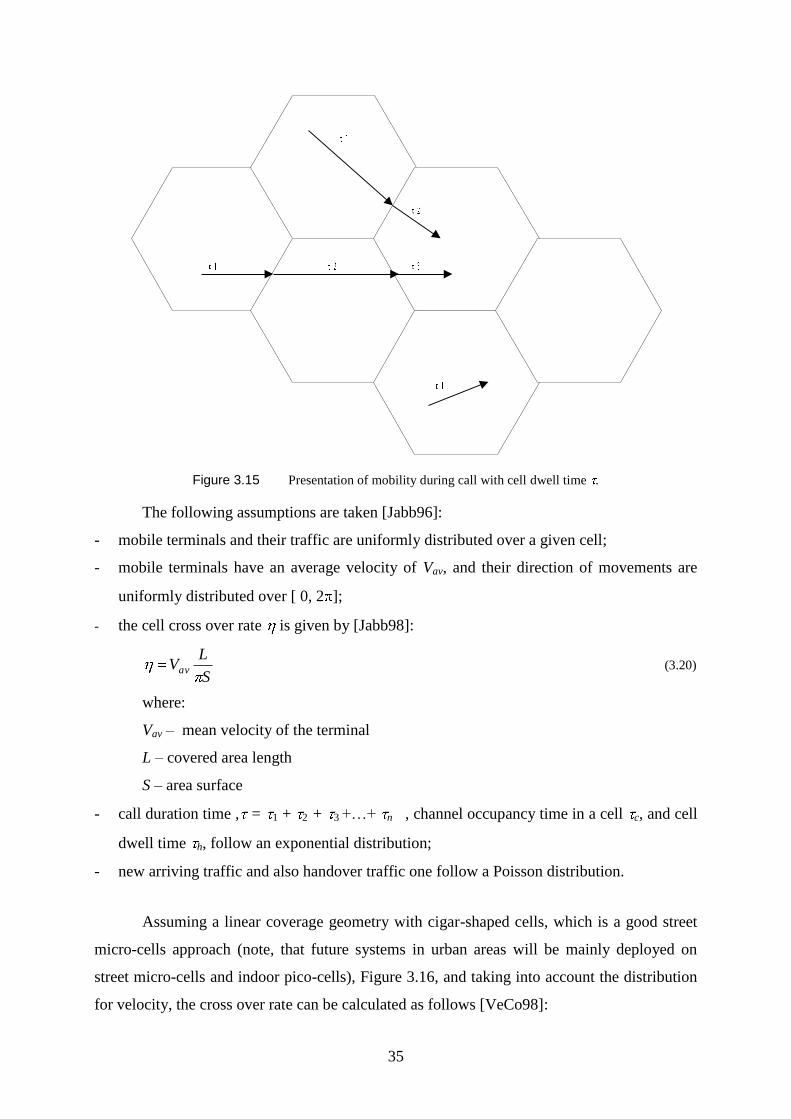
35
Figure 3.15 Presentation of mobility during call with cell dwell time .
The following assumptions are taken [Jabb96]:
- mobile terminals and their traffic are uniformly distributed over a given cell;
- mobile terminals have an average velocity of Vav, and their direction of movements are
uniformly distributed over [ 0, 2 ];
- the cell cross over rate is given by [Jabb98]:
S
LVav (3.20)
where:
Vav – mean velocity of the terminal
L – covered area length
S – area surface
- call duration time , = 1 + 2 + 3 +…+ n , channel occupancy time in a cell c, and cell
dwell time h, follow an exponential distribution;
- new arriving traffic and also handover traffic one follow a Poisson distribution.
Assuming a linear coverage geometry with cigar-shaped cells, which is a good street
micro-cells approach (note, that future systems in urban areas will be mainly deployed on
street micro-cells and indoor pico-cells), Figure 3.16, and taking into account the distribution
for velocity, the cross over rate can be calculated as follows [VeCo98]:
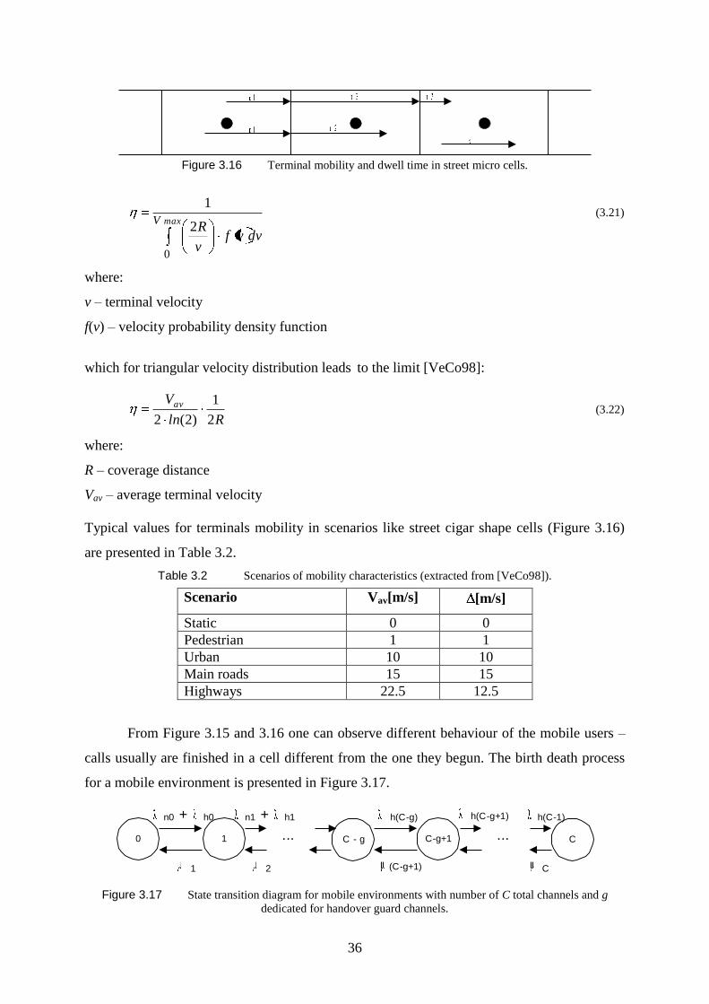
36
Figure 3.16 Terminal mobility and dwell time in street micro cells.
maxV
dvvfv
R
0
2
1 (3.21)
where:
v – terminal velocity
f(v) – velocity probability density function
which for triangular velocity distribution leads to the limit [VeCo98]:
Rln
Vav
2
1
)2(2 (3.22)
where:
R – coverage distance
Vav – average terminal velocity
Typical values for terminals mobility in scenarios like street cigar shape cells (Figure 3.16)
are presented in Table 3.2.
Table 3.2 Scenarios of mobility characteristics (extracted from [VeCo98]).
Scenario Vav[m/s] [m/s]
Static 0 0
Pedestrian 1 1
Urban 10 10
Main roads 15 15
Highways 22.5 12.5
From Figure 3.15 and 3.16 one can observe different behaviour of the mobile users –
calls usually are finished in a cell different from the one they begun. The birth death process
for a mobile environment is presented in Figure 3.17.
0 CC-g+1C - g1
(C-g+1)21
...
n0 h0+ n1 h1+
C
...
h(C-g+1) h(C-1)h(C-g)
Figure 3.17 State transition diagram for mobile environments with number of C total channels and g
dedicated for handover guard channels.
37
The mean dwell time h can be estimated by knowing the cell cross over rate [Jabb96]:
1h (3.23)
The channel occupancy time c = min{ , h }is the time spent in cell before crossing the cell
boundary if the call continues. It is the minimum of two exponentially distributed random
variables, thus being also exponentially distributed with service rate, c = + . It is
important noting that service rate c represents now the channel holding (occupancy) time in a
cell, previously represented by (when mobility was not considered).
Therefore, the mean channel occupancy time c for a new or handover call is given by
[Jabb96]:
1c (3.24)
The probability of handover, Ph, is being given by [VeCo98]:
h
c
c
hh TPP (3.25)
The total offered traffic to a cell is dependent on the handover traffic, which is turn depends
on the total offered traffic to a cell. Using the flow equilibrium property, one can write
[Jabb96]:
nhfnbhh PPP 11 (3.26)
where:
Phf – probability of handover failure
which can be approximated for small values of Pb and Phf as follows [Jabb96]:
nn
h
hh
P
P
1 (3.27)
The total new arriving traffic in cell in mobile scenarios is represented by:
hn AAA (3.28)
where:
Ah – traffic incoming from handover: Ah = h/ c
An – new arriving traffic: An = n/ c
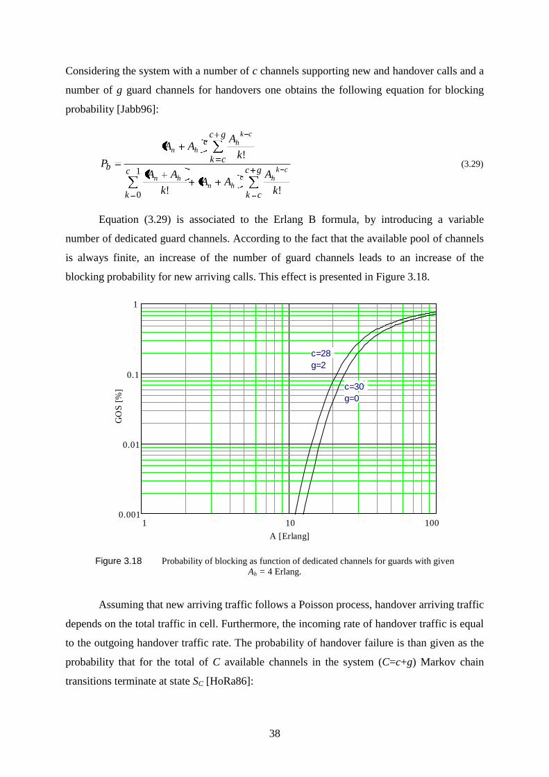
38
Considering the system with a number of c channels supporting new and handover calls and a
number of g guard channels for handovers one obtains the following equation for blocking
probability [Jabb96]:
1
0 !!
!
c
k
gc
ck
gc
ck
c
b
k
AAA
k
AA
k
AAA
Pck
hchn
hn
ck
hhn
(3.29)
Equation (3.29) is associated to the Erlang B formula, by introducing a variable
number of dedicated guard channels. According to the fact that the available pool of channels
is always finite, an increase of the number of guard channels leads to an increase of the
blocking probability for new arriving calls. This effect is presented in Figure 3.18.
1 10 1000.001
0.01
0.1
1
A [Erlang]
GO
S [
%]
c=28
g=2
c=30
g=0
Figure 3.18 Probability of blocking as function of dedicated channels for guards with given
Ah = 4 Erlang.
Assuming that new arriving traffic follows a Poisson process, handover arriving traffic
depends on the total traffic in cell. Furthermore, the incoming rate of handover traffic is equal
to the outgoing handover traffic rate. The probability of handover failure is than given as the
probability that for the total of C available channels in the system (C=c+g) Markov chain
transitions terminate at state SC [HoRa86]:
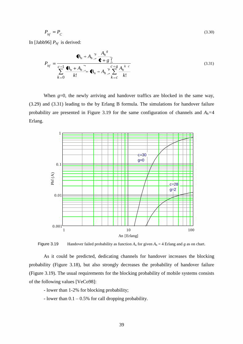
39
ChfPP (3.30)
In [Jabb96] Phf is derived:
1
0 !!
!
c
k
gc
ck k
AAA
k
AA
gc
AAA
Pck
hchn
hn
ghc
hn
hf (3.31)
When g=0, the newly arriving and handover traffics are blocked in the same way,
(3.29) and (3.31) leading to the by Erlang B formula. The simulations for handover failure
probability are presented in Figure 3.19 for the same configuration of channels and Ah=4
Erlang.
1 10 1000.001
0.01
0.1
1
An [Erlang]
Ph
f (A
)
c=30
g=0
c=28
g=2
Figure 3.19 Handover failed probability as function An for given Ah = 4 Erlang and g as on chart.
As it could be predicted, dedicating channels for handover increases the blocking
probability (Figure 3.18), but also strongly decreases the probability of handover failure
(Figure 3.19). The usual requirements for the blocking probability of mobile systems consists
of the following values [VeCo98]:
- lower than 1-2% for blocking probability;
- lower than 0.1 – 0.5% for call dropping probability.
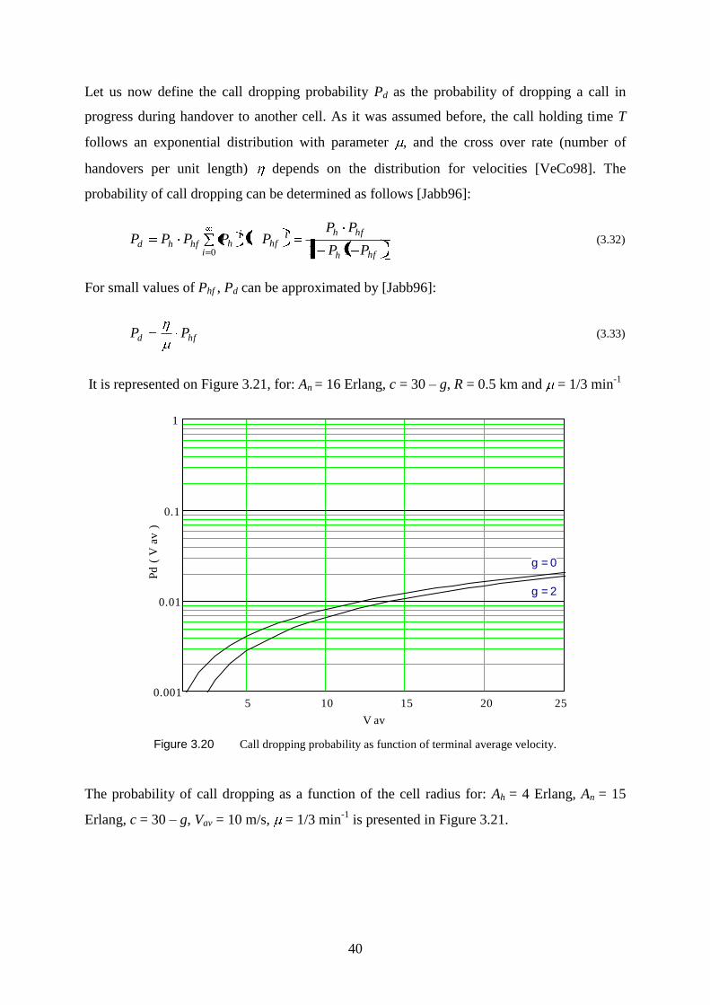
40
Let us now define the call dropping probability Pd as the probability of dropping a call in
progress during handover to another cell. As it was assumed before, the call holding time T
follows an exponential distribution with parameter , and the cross over rate (number of
handovers per unit length) depends on the distribution for velocities [VeCo98]. The
probability of call dropping can be determined as follows [Jabb96]:
hfh
hfh
hfi
hhfhdPP
PPPPPPP ii
111
0
(3.32)
For small values of Phf , Pd can be approximated by [Jabb96]:
hfd PP (3.33)
It is represented on Figure 3.21, for: An = 16 Erlang, c = 30 – g, R = 0.5 km and = 1/3 min-1
5 10 15 20 250.001
0.01
0.1
1
V av
Pd
( V
av
)
g = 0
g = 2
Figure 3.20 Call dropping probability as function of terminal average velocity.
The probability of call dropping as a function of the cell radius for: Ah = 4 Erlang, An = 15
Erlang, c = 30 – g, Vav = 10 m/s, = 1/3 min-1
is presented in Figure 3.21.
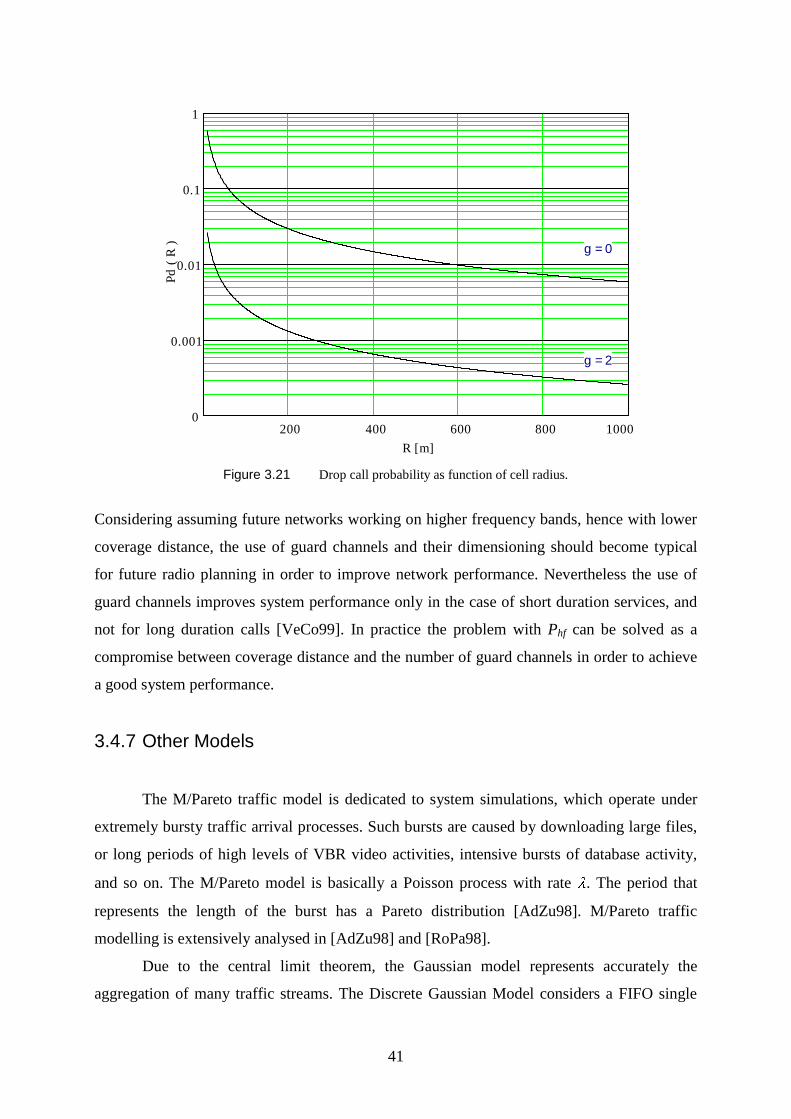
41
200 400 600 800 10000
0.001
0.01
0.1
1
R [m]
Pd
( R
) g = 0
g = 2
Figure 3.21 Drop call probability as function of cell radius.
Considering assuming future networks working on higher frequency bands, hence with lower
coverage distance, the use of guard channels and their dimensioning should become typical
for future radio planning in order to improve network performance. Nevertheless the use of
guard channels improves system performance only in the case of short duration services, and
not for long duration calls [VeCo99]. In practice the problem with Phf can be solved as a
compromise between coverage distance and the number of guard channels in order to achieve
a good system performance.
3.4.7 Other Models
The M/Pareto traffic model is dedicated to system simulations, which operate under
extremely bursty traffic arrival processes. Such bursts are caused by downloading large files,
or long periods of high levels of VBR video activities, intensive bursts of database activity,
and so on. The M/Pareto model is basically a Poisson process with rate . The period that
represents the length of the burst has a Pareto distribution [AdZu98]. M/Pareto traffic
modelling is extensively analysed in [AdZu98] and [RoPa98].
Due to the central limit theorem, the Gaussian model represents accurately the
aggregation of many traffic streams. The Discrete Gaussian Model considers a FIFO single
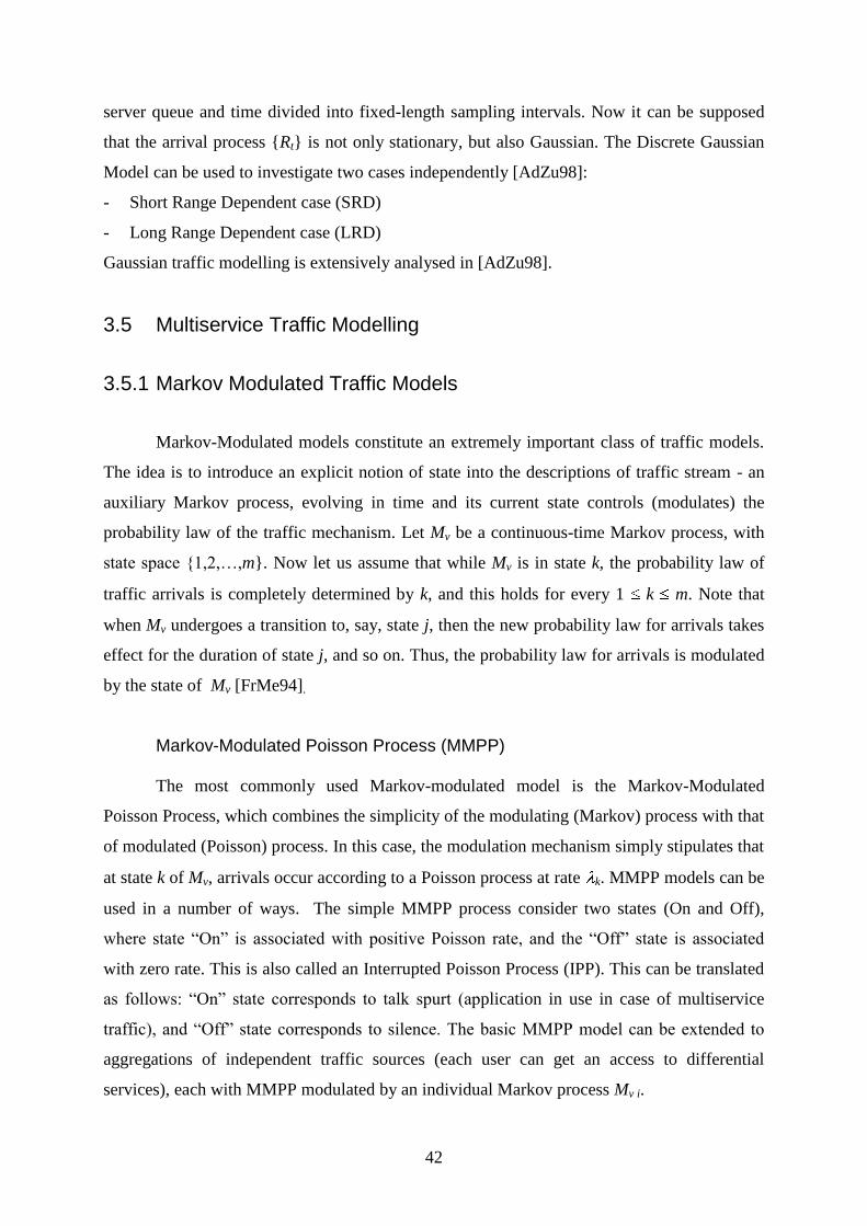
42
server queue and time divided into fixed-length sampling intervals. Now it can be supposed
that the arrival process {Rt} is not only stationary, but also Gaussian. The Discrete Gaussian
Model can be used to investigate two cases independently [AdZu98]:
- Short Range Dependent case (SRD)
- Long Range Dependent case (LRD)
Gaussian traffic modelling is extensively analysed in [AdZu98].
3.5 Multiservice Traffic Modelling
3.5.1 Markov Modulated Traffic Models
Markov-Modulated models constitute an extremely important class of traffic models.
The idea is to introduce an explicit notion of state into the descriptions of traffic stream - an
auxiliary Markov process, evolving in time and its current state controls (modulates) the
probability law of the traffic mechanism. Let Mv be a continuous-time Markov process, with
state space {1,2,…,m}. Now let us assume that while Mv is in state k, the probability law of
traffic arrivals is completely determined by k, and this holds for every 1 k m. Note that
when Mv undergoes a transition to, say, state j, then the new probability law for arrivals takes
effect for the duration of state j, and so on. Thus, the probability law for arrivals is modulated
by the state of Mv [FrMe94].
Markov-Modulated Poisson Process (MMPP)
The most commonly used Markov-modulated model is the Markov-Modulated
Poisson Process, which combines the simplicity of the modulating (Markov) process with that
of modulated (Poisson) process. In this case, the modulation mechanism simply stipulates that
at state k of Mv, arrivals occur according to a Poisson process at rate k. MMPP models can be
used in a number of ways. The simple MMPP process consider two states (On and Off),
where state “On” is associated with positive Poisson rate, and the “Off” state is associated
with zero rate. This is also called an Interrupted Poisson Process (IPP). This can be translated
as follows: “On” state corresponds to talk spurt (application in use in case of multiservice
traffic), and “Off” state corresponds to silence. The basic MMPP model can be extended to
aggregations of independent traffic sources (each user can get an access to differential
services), each with MMPP modulated by an individual Markov process Mv i.
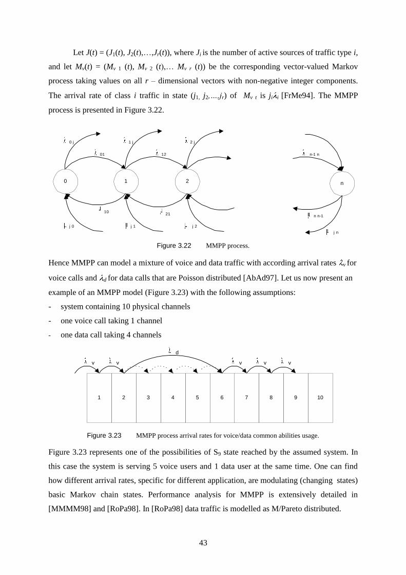
43
Let J(t) = (J1(t), J2(t),…,Jr(t)), where Ji is the number of active sources of traffic type i,
and let Mv(t) = (Mv 1 (t), Mv 2 (t),… Mv r (t)) be the corresponding vector-valued Markov
process taking values on all r – dimensional vectors with non-negative integer components.
The arrival rate of class i traffic in state (j1, j2,…,jr) of Mv t is ji i [FrMe94]. The MMPP
process is presented in Figure 3.22.
0 1 2 n
01
10
1 j0 j
12
2 j
j 0 j 1
n n-121
n-1 n
j 2
j n
Figure 3.22 MMPP process.
Hence MMPP can model a mixture of voice and data traffic with according arrival rates v for
voice calls and d for data calls that are Poisson distributed [AbAd97]. Let us now present an
example of an MMPP model (Figure 3.23) with the following assumptions:
- system containing 10 physical channels
- one voice call taking 1 channel
- one data call taking 4 channels
1 5432 76 8 9 10
v v vv v
d
Figure 3.23 MMPP process arrival rates for voice/data common abilities usage.
Figure 3.23 represents one of the possibilities of S9 state reached by the assumed system. In
this case the system is serving 5 voice users and 1 data user at the same time. One can find
how different arrival rates, specific for different application, are modulating (changing states)
basic Markov chain states. Performance analysis for MMPP is extensively detailed in
[MMMM98] and [RoPa98]. In [RoPa98] data traffic is modelled as M/Pareto distributed.
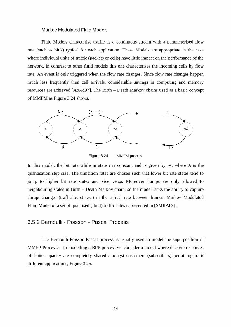
44
Markov Modulated Fluid Models
Fluid Models characterise traffic as a continuous stream with a parameterised flow
rate (such as bit/s) typical for each application. These Models are appropriate in the case
where individual units of traffic (packets or cells) have little impact on the performance of the
network. In contrast to other fluid models this one characterises the incoming cells by flow
rate. An event is only triggered when the flow rate changes. Since flow rate changes happen
much less frequently then cell arrivals, considerable savings in computing and memory
resources are achieved [AbAd97]. The Birth – Death Markov chains used as a basic concept
of MMFM as Figure 3.24 shows.
0 A 2A NA
Figure 3.24 MMFM process.
In this model, the bit rate while in state i is constant and is given by iA, where A is the
quantisation step size. The transition rates are chosen such that lower bit rate states tend to
jump to higher bit rate states and vice versa. Moreover, jumps are only allowed to
neighbouring states in Birth – Death Markov chain, so the model lacks the ability to capture
abrupt changes (traffic burstiness) in the arrival rate between frames. Markov Modulated
Fluid Model of a set of quantised (fluid) traffic rates is presented in [SMRA89].
3.5.2 Bernoulli - Poisson - Pascal Process
The Bernoulli-Poisson-Pascal process is usually used to model the superposition of
MMPP Processes. In modelling a BPP process we consider a model where discrete resources
of finite capacity are completely shared amongst customers (subscribers) pertaining to K
different applications, Figure 3.25.
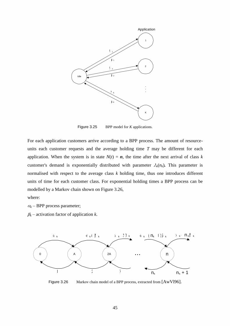
45
Idle
1
K
2
Application
.
.
.
1
K
2
K
1
2
Figure 3.25 BPP model for K applications.
For each application customers arrive according to a BPP process. The amount of resource-
units each customer requests and the average holding time T may be different for each
application. When the system is in state N(t) = n, the time after the next arrival of class k
customer's demand is exponentially distributed with parameter k(nk). This parameter is
normalised with respect to the average class k holding time, thus one introduces different
units of time for each customer class. For exponential holding times a BPP process can be
modelled by a Markov chain shown on Figure 3.26,
where:
k – BPP process parameter;
k – activation factor of application k.
0 A 2A n
n
k kkkk k n k k
k
n k k k
n + 1k
...
Figure 3.26 Markov chain model of a BPP process, extracted from [AwVl96].
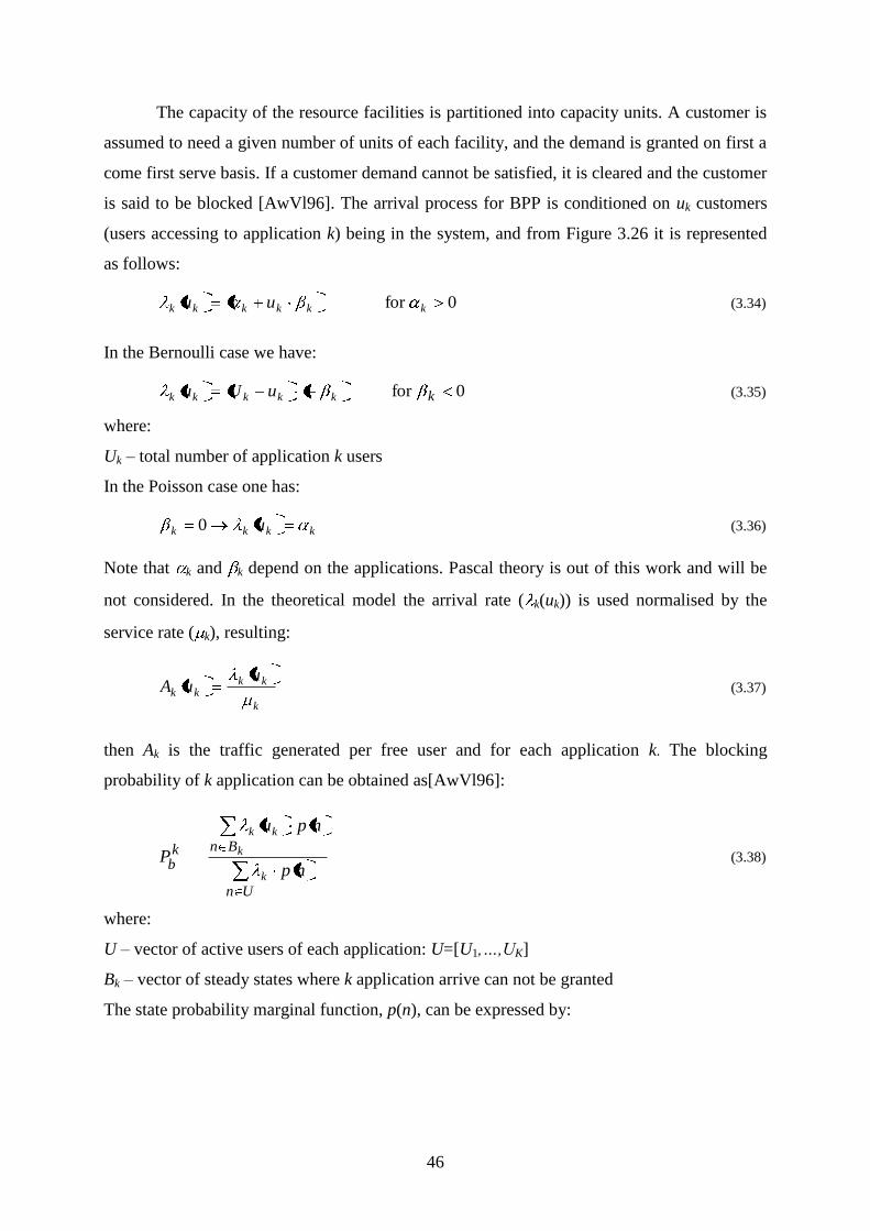
46
The capacity of the resource facilities is partitioned into capacity units. A customer is
assumed to need a given number of units of each facility, and the demand is granted on first a
come first serve basis. If a customer demand cannot be satisfied, it is cleared and the customer
is said to be blocked [AwVl96]. The arrival process for BPP is conditioned on uk customers
(users accessing to application k) being in the system, and from Figure 3.26 it is represented
as follows:
0for kkkkkk uu (3.34)
In the Bernoulli case we have:
0for kkkkkk uUu (3.35)
where:
Uk – total number of application k users
In the Poisson case one has:
kkkk u0 (3.36)
Note that k and k depend on the applications. Pascal theory is out of this work and will be
not considered. In the theoretical model the arrival rate ( k(uk)) is used normalised by the
service rate ( k), resulting:
k
kkkk
uuA (3.37)
then Ak is the traffic generated per free user and for each application k. The blocking
probability of k application can be obtained as[AwVl96]:
Un
Bnkb np
npu
Pk
k
kk
(3.38)
where:
U – vector of active users of each application: U=[U1,…,UK]
Bk – vector of steady states where k application arrive can not be granted
The state probability marginal function, p(n), can be expressed by:
47
Un
K
k
K
k
kk
kk
uv
uv
np
1
1 for n U (3.39)
where the unnormalised marginal probabilities, vk(uk) are:
kk
k
k
kku
U
u
uv for the Bernoulli case;
(3.40)
!uuv
k
kk
n
kk for the Poisson case.
System Average Load
If there is a total number of C available resources in each cell being used by a number
of M users, each user can be either in an idle state or using one of the applications, k=1,2,...,K
with generation and total service rates, k and k , respectively and with a proportion among
all the applications of propk
11
K
kkprop (3.41)
The proportion of users of an application among all the available ones can be expressed like:
K
ii
kk
A
Aprop
1
(3.42)
where:
kk propAA
(3.43)
K
iiAA
1
In [Vele99] one can find the following formula for the probability of an user having an active
application k:
48
kkk
k propfpropA
A
A
Ap
K
ii
11
1
(3.44)
where:
the fraction of active users f = A / (1+A)
In teletraffic usually one is interested in obtaining the blocking probability as a function of the
average load. The load from each user is obtained by computing the expectation of every
application data rate [Vele99]:
K
iiiu bpL
1
(3.45)
where:
bi – application i data rate.
pi – probability of a user having application i opened
The load from each user lead to the system average load (multiplying by M):
McfMLL u 1 (3.46)
where:
K
iii bpropc
11 (3.47)
The parameter c1 gives information about the maximal resources that will be used by each
user when f=1 i.e., maximal load per user, which leads to the best understanding of the system
behaviour.
Equivalent User
Now, if the applications have access to different service components, equivalent users
should be considered. An application k equivalent user is composed by a set of the service
components virtual users (service components are HDTV, Data, high quality pictures, etc.),
which arise according to application's activation. The activation of service components is
presented in Figure 3.27
49
Idle
1 .
.
.
1
K
2
K
1
2 2
K
1
J
1\ 1
J\1
J\1
1\ 1
Service component j used
by appl ication kApplication activation
.
.
.
Figure 3.27 Service components activation.
Each service component uses resources with its required data rates aj, and exponentially
distributed holding time. While the application k is active, the service components are
activated with rate j\k and extinguished with total service rate j\k, j=1,2,…,J (Figure 3.27)
they can be simultaneously active, or not. This is a loss system, whose performance can be
measured by the blocking probability of each service component. For service activation the
Bernoulli model is used (Figure 3.28), because of [Vele99]:
- the population accessing to service components is assumed small and it correctly models
the reduction of the call arrival intensity when the number of active users increase;
- activation of each service component is independent.
The activation rate of each component given an application k is defined by [Vele99]:
k
k\jk\j
/
n
1 (3.48)
where:
nj\k – average number of active service component j request
When the system is in state N(t) = n, the time after the next arrival of class j customer's arrival
is exponentially distributed with parameter j(nj). This parameter is normalised with respect to
the average class k holding time, thus one introduces a different unit of time for each
customer class. The arrival rate is represented as follows [Vele99].
50
jjjjjjjj uUnu (3.49)
where:
Uj – total number of component j users
uj – number of users accessing to service component j
In the Bernoulli case, where (- j) is the activation rate of the component j (Figure 3.28), j=-
j Uj, where Uj is equal to the total number of system users M. As it was said before, these
parameters should be normalised with respect of the total service rate of component j,
meaning that different time scales should be introduced for each j, thus j' = j / j and
j'= j' Uj.
Idle Activ e
j
j
Service component j
activation
Figure 3.28 Service components activation according to Bernoulli model (extracted from [Vele99]).
The activation rate of service component j is given by [Vele99]:
kk\jkk\jj proppK
k
K
k 11 1 (3.50)
If the system is stationary, the average occupancy of service component j is given by
[Vele99]:
k
K
k\j
k\j
j
j
j pk 1
(3.51)
The normalised average occupancy of service component j is given by [Vele99]:
K
k
*
K
k
*
k
k
k\j
k\j
k
kk\j
j
1
1 (3.52)
where:
kkk prop* (3.53)
51
The data rates associated with each application are [Vele99]:
J
jj
k
k\j
k\j
k a
n
b1
1
1
(3.54)
where:
aj – service component j data rates
If the influence of application mobility is taken into account the arrival rate k is the
sum of arriving in cell traffic and traffic from handover.
k
kk
nkhknk (3.55)
Consequently the mobility of system users has influence on each component handover failure
probability, and it can be given approximately by [Vele99]:
maxd
j
j
jhf PP (3.56)
where:
(Pd)max – maximum allowed dropping probability
Independence in service components activation during application service time is
assumed, allowing the BPP process described above to capture traffic burstiness. Thus it can
correctly model MMPP in future multiservice networks.

52
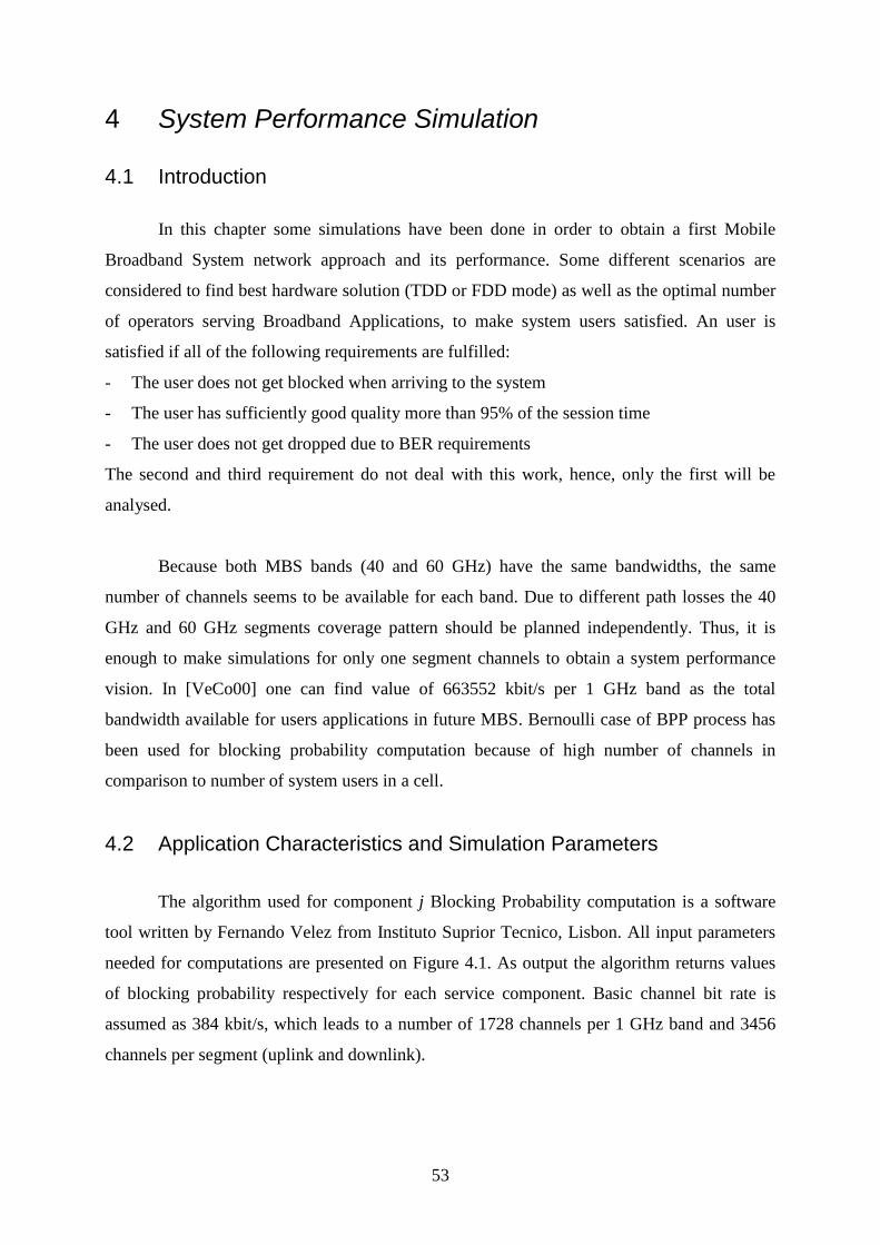
53
4 System Performance Simulation
4.1 Introduction
In this chapter some simulations have been done in order to obtain a first Mobile
Broadband System network approach and its performance. Some different scenarios are
considered to find best hardware solution (TDD or FDD mode) as well as the optimal number
of operators serving Broadband Applications, to make system users satisfied. An user is
satisfied if all of the following requirements are fulfilled:
- The user does not get blocked when arriving to the system
- The user has sufficiently good quality more than 95% of the session time
- The user does not get dropped due to BER requirements
The second and third requirement do not deal with this work, hence, only the first will be
analysed.
Because both MBS bands (40 and 60 GHz) have the same bandwidths, the same
number of channels seems to be available for each band. Due to different path losses the 40
GHz and 60 GHz segments coverage pattern should be planned independently. Thus, it is
enough to make simulations for only one segment channels to obtain a system performance
vision. In [VeCo00] one can find value of 663552 kbit/s per 1 GHz band as the total
bandwidth available for users applications in future MBS. Bernoulli case of BPP process has
been used for blocking probability computation because of high number of channels in
comparison to number of system users in a cell.
4.2 Application Characteristics and Simulation Parameters
The algorithm used for component j Blocking Probability computation is a software
tool written by Fernando Velez from Instituto Suprior Tecnico, Lisbon. All input parameters
needed for computations are presented on Figure 4.1. As output the algorithm returns values
of blocking probability respectively for each service component. Basic channel bit rate is
assumed as 384 kbit/s, which leads to a number of 1728 channels per 1 GHz band and 3456
channels per segment (uplink and downlink).
54
Algorithmn
j\k
j\k
k
propk
Pb j
C aj
U
Scenario
Figure 4.1 Algorithm input and output parameters.
Seeing MBS as a system generally deployed in large agglomerations the following
environments can be specified [VeCo00]:
- business city centre BCC
- urban URB
- main roads ROA
Each scenario can be characterised by another set of values of the following
parameters: proportion of applications users propk, average application usage time 1/ k,
application burstiness nj\k seen as a number of access requests to service components during
application usage, service components average usage time 1/ j\k. As a consequence different
asymmetry factors AF between uplink and downlink can be expected for each scenario. The
service components have different bandwidth requirements which can be specified as a
number of basic channels from the total C available requested to serve service component j.
The main future MBS applications and their parameters are extracted from [VeCo00] and
presented in Table 4.1 and Table 4.2.
55
Table 4.1 Main MBS applications transmission parameters.
Application
Abbreviation
Burstiness
Time
dependency
Delivery
requirements
Symmetry/
Asymmetry
1 HD Video-telephony HVT 1-5
TB
RT
Sym/Asy
2 ISDN Videoconference IVC 1-5
3 Mobile Video Surveillance MVS 1-5
Asy 4 HDTV Outside Broadcast HOB 1-5
5 Wireless LAN Interconnection WLI 1-50 NRT/RT
6 Data File Transfer FTP 1-50 NTB RT
7 Professional Images PIM 1-20 TB/NTB RT
8 Desktop Multimedia DMM 1-20
TB
RT 9 Mobile Emergency Services MES 1-5 Sym
10 Mobile Repair Assistance MRA 1-5
11 Mobile Tele-working MTW 1-20
12 Freight and Fleet Management FFM 1-5
13 Electronic Mailbox Service for
Multimedia
EMB 1-20 TB NRT Asy
14 E-commerce ECO 1-20 TB
RT
Asy 15 Multimedia Library MML 1-20
16 Tourist Information TIN 1-20 NTB
17 Remote Procedure Call RPC 1-50
NRT/RT 18 Urban Guidance UGD 1-5 TB
19 Assistance in Travel ATR 1-5
20 TV Programme Distribution TVD 1 TB RT -
21 E-newspaper ENP 1-20 TB NRT Asy
Table 4.2 Average duration and proportion of application users in different scenarios.
Application 1/ k
[min]
BCC URB ROA
propk propk propk
1 HVT 3 0.15 0.11 0.098
2 IVC 30 0.04 0.04 0.04
3 MVS 120 0.004 0.005 0.002
4 HOB 50 0.001 0.001 0.001
5 WLI 15 0.054 0.021 0.056
6 FTP 0.33 0.07 0.07 0.07
7 PIM 10 0.02 0.01 0.015
8 DMM 5 0.15 0.15 0.15
9 MES 20 0.018 0.001 0.016
10 MRA 40 0.002 0.001 0.003
11 MTW 20 0.073 0.022 0.033
12 FFM 5 0.007 0.002 0.023
13 EMB 1 0.03 0.03 0.02
14 ECO 5 0.07 0.07 0.07
15 MML 40 0.074 0.044 0.056
16 TIN 15 0.036 0.01 0.021
17 RPC 5 0.03 0.08 0.03
18 UGD 5 0.011 0.033 0.033
19 ATR 20 0.036 0.11 0.163
20 TVD 90 0.074 0.09 0.05
21 ENP 20 0.05 0.1 0.05
56
As it was previously remarked MBS is seen as an UMTS extension to Broadband
ISDN Services, so in a natural way each operator of UMTS should get in the future license for
MBS. Table 4.3 presents the consequence of such policy. Only in the first scenario (2
operators using reuse pattern 2) 155 Mbit/s per user is reachable for FDD mode.
Table 4.3 Number of 384 kbit/s channels available in a cell for different scenarios.
Number of Operators 2 3 4 5 6
Reuse Pattern 2 3 4 5 2 3 4 5 2 3 4 5 2 3 4 5 2 3 4 5
No of channels in Uplink 432 288 216 173 288 192 144 115 216 144 108 86 173 115 86 69 144 96 72 58
No of channels in Downlink 432 288 216 173 288 192 144 115 216 144 108 86 173 115 86 69 144 96 72 58
In [VeCo00] some analysis concerning the optimal number of service components and
their bandwidth (thus channel requirements) has been done. The preferred bit rates
requirements are the ones presented in Table 4.4.
Table 4.4 Service components and their bandwidth request.
Service component j aj Rbs j
[kbit/s]
BAS 1 1 384
MED1 2 3 1152
MED2 3 4 1536
MED3 4 5 1920
HDV 5 21 8064
HID 6 83 31872
The usage of service components by applications is characterised by two parameters:
- number of request of application k service component j (application burstiness) n j\k
- average service rate (usage time) of service component by application j\k
If the application access to service component is permanent, such case parameter n j\k = 1 and
the application average usage time is equal to relevant average service component usage time
(1/ k = 1/ j\k). Such situation occurs in the case of real time applications like
videoconferencing and video broadcasting. The values used in simulations are extracted from
[VeCo00] and presented in Tables 4.5 – 4.8.
57
Table 4.5 Parameter n j\k for uplink.
Application n j\k
BAS MED1 MED2 MED3 HDV HID
1 HVT 0 0 0 1 0 0
2 IVC 1 0 0 0 0 0
3 MVS 0 0 0 1 0 0
4 HOB 0 20 0 0 1 0
5 WLI 0 34.5 0 0 0 0
6 FTP 2 0 0 0 0 0
7 PIM 1 0 0 0 0 0
8 DMM 15 0 0 0 0 0
9 MES 0 10 0 1 4 0
10 MRA 0 20 0 1 4 0
11 MTW 0 20 0 1 0 0
12 FFM 0 5 0 1 1 0
13 EMB 3 0 0 0 0 0
14 ECO 25 0 0 0 0 0
15 MML 0 20 0 0 0 0
16 TIN 0 120 0 0 0 0
17 RPC 0 5 0 0 0 0
18 UGD 0 8 0 1 0 0
19 ATR 0 30 0 1 0 0
20 TVD 0 0 0 0 0 0
21 ENP 5 0 0 0 0 0
Table 4.6 Parameter j\k for uplink.
Application 1/ j\k
[min]
BAS MED1 MED2 MED3 HDV HID
1 HVT 0 0 0 3 0 0
2 IVC 30 0 0 0 0 0
3 MVS 0 0 0 120 0 0
4 HOB 0 0.0083 0 0 50 0
5 WLI 0 0.055 0 0 0 0
6 FTP 0.0083 0 0 0 0 0
7 PIM 10 0 0 0 0 0
8 DMM 0.055 0 0 0 0 0
9 MES 0 0.0083 0 20 0.5 0
10 MRA 0 0.0083 0 40 0.5 0
11 MTW 0 0.0083 0 20 0 0
12 FFM 0 0.0083 0 5 0.5 0
13 EMB 0.055 0 0 0 0 0
14 ECO 0.0083 0 0 0 0 0
15 MML 0 0.0083 0 0 0 0
16 TIN 0 0.0083 0 0 0 0
17 RPC 0 0.0083 0 0 0 0
18 UGD 0 0.0083 0 5 0 0
19 ATR 0 0.0083 0 20 0 0
20 TVD 0 0 0 0 0 0
21 ENP 0.0083 0 0 0 0 0
58
Table 4.7 Parameter n j\k for downlink.
Application n j\k
BAS MED1 MED2 MED3 HDV HID
1 HVT 0 0 0 1 0 0
2 IVC 1 0 0 0 0 0
3 MVS 30 0 0 0 0 0
4 HOB 0 20 0 1 0 0
5 WLI 0 0 0 0 0 34.5
6 FTP 1 0 0 0 0 0
7 PIM 0 0 0 0 1 0
8 DMM 11.5 0 0 0 0 0
9 MES 0 10 0 1 4 0
10 MRA 0 20 0 1 4 0
11 MTW 0 20 0 1 0 0
12 FFM 0 5 0 1 1 0
13 EMB 0 0 1 0 0 0
14 ECO 11.5 0 0 0 0 0
15 MML 0 20 0 1 4 0
16 TIN 0 0 0 34.5 0 0
17 RPC 0 0 11.5 0 0 0
18 UGD 0 8 0 1 0 0
19 ATR 0 30 0 1 0 0
20 TVD 0 0 0 0 1 0
21 ENP 0 0 0 46 0 0
Table 4.8 Parameter j\k for uplink.
Application 1/ j\k
[min] BAS MED1 MED2 MED3 HDV HID
1 HVT 0 0 0 3 0 0
2 IVC 30 0 0 0 0 0
3 MVS 0.0083 0 0 0 0 0
4 HOB 0 0.0083 0 50 0 0
5 WLI 0 0 0 0 0 0.055
6 FTP 0.33 0 0 0 0 0
7 PIM 0 0 0 0 10 0
8 DMM 0.055 0 0 0 0 0
9 MES 0 0.0083 0 20 0.5 0
10 MRA 0 0.0083 0 40 0.5 0
11 MTW 0 0.0083 0 20 0 0
12 FFM 0 0.0083 0 5 0.5 0
13 EMB 0 0 1 0 0 0
14 ECO 0.055 0 0 0 0 0
15 MML 0 0.0083 0 40 0.5 0
16 TIN 0 0 0 0.055 0 0
17 RPC 0 0 0.055 0 0 0
18 UGD 0 0.0083 0 5 0 0
19 ATR 0 0.0083 0 20 0 0
20 TVD 0 0 0 0 90 0
21 ENP 0 0 0 0.055 0 0
59
Results
In this section some results are obtained for different environments and scenarios in
order to show the first system performance approach. The blocking probability is represented
as a fraction of active users in a cell. Four pools of the numbers of potential users, M in a cell
are considered: 100, 166, 250 and 500 users. Thus, a traffic engineer while knowing the
forecasted number of subscribers in the considered area, can make cell capacity dimensioning,
hence preparing base stations raster referring to acceptable path loss for choosing the working
frequency. Optimisation of the existing system in terms of a better utilisation of channels can
be done as well.
A number of 216 channels has been chosen both for uplink and downlink in order to
prepare the set of simulations. The obtained results for such a symmetric case, in different
environments are presented in Figures 4.2, 4.3 and 4.4. This value of 216 channels in the
system, fulfilling some scenarios, can be referred results to other scenarios, which are
characterised by a similar number of available channels (e.g., 3 operators with re-use pattern 3
implies a number of 192 available channels both for uplink and downlink).
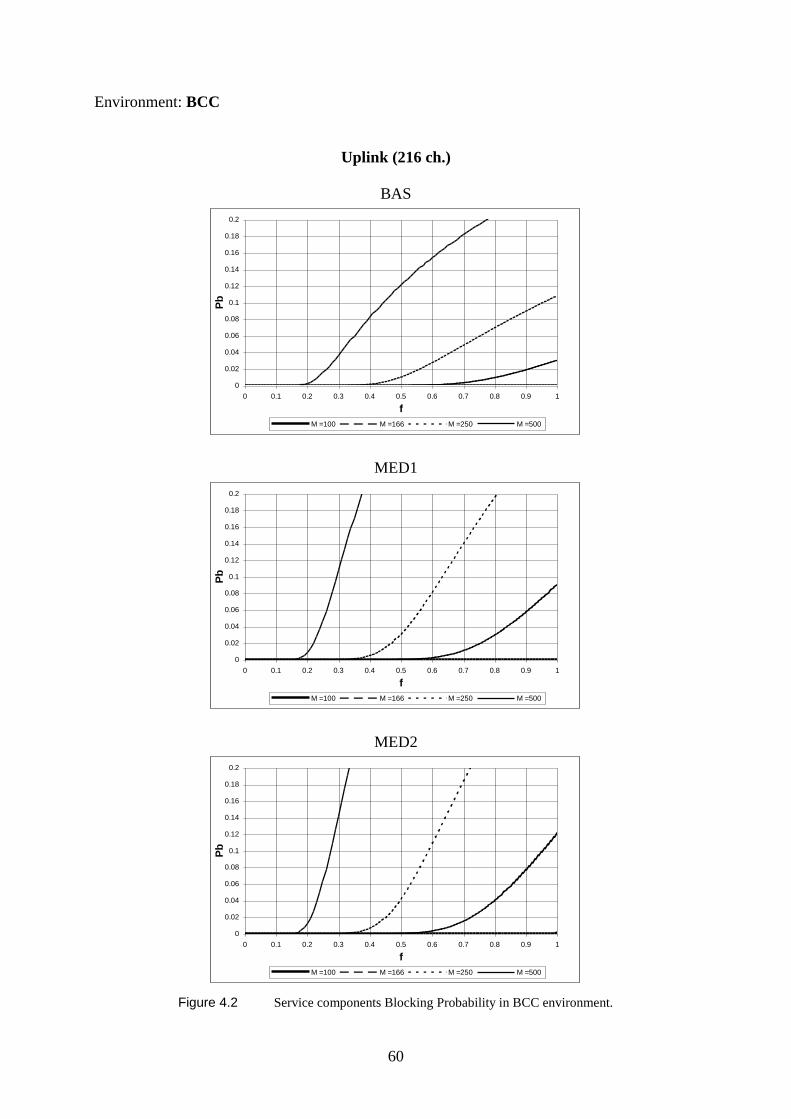
60
Environment: BCC
Uplink (216 ch.)
BAS
0
0.02
0.04
0.06
0.08
0.1
0.12
0.14
0.16
0.18
0.2
0 0.1 0.2 0.3 0.4 0.5 0.6 0.7 0.8 0.9 1
f
Pb
M =100 M =166 M =250 M =500
MED1
0
0.02
0.04
0.06
0.08
0.1
0.12
0.14
0.16
0.18
0.2
0 0.1 0.2 0.3 0.4 0.5 0.6 0.7 0.8 0.9 1
f
Pb
M =100 M =166 M =250 M =500
MED2
0
0.02
0.04
0.06
0.08
0.1
0.12
0.14
0.16
0.18
0.2
0 0.1 0.2 0.3 0.4 0.5 0.6 0.7 0.8 0.9 1
f
Pb
M =100 M =166 M =250 M =500
Figure 4.2 Service components Blocking Probability in BCC environment.
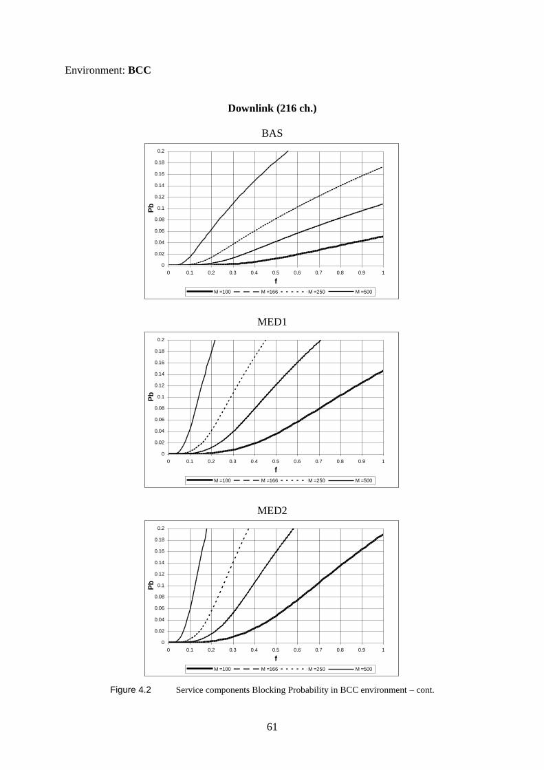
61
Environment: BCC
Downlink (216 ch.)
BAS
0
0.02
0.04
0.06
0.08
0.1
0.12
0.14
0.16
0.18
0.2
0 0.1 0.2 0.3 0.4 0.5 0.6 0.7 0.8 0.9 1
f
Pb
M =100 M =166 M =250 M =500
MED1
0
0.02
0.04
0.06
0.08
0.1
0.12
0.14
0.16
0.18
0.2
0 0.1 0.2 0.3 0.4 0.5 0.6 0.7 0.8 0.9 1
f
Pb
M =100 M =166 M =250 M =500
MED2
0
0.02
0.04
0.06
0.08
0.1
0.12
0.14
0.16
0.18
0.2
0 0.1 0.2 0.3 0.4 0.5 0.6 0.7 0.8 0.9 1
f
Pb
M =100 M =166 M =250 M =500
Figure 4.2 Service components Blocking Probability in BCC environment – cont.
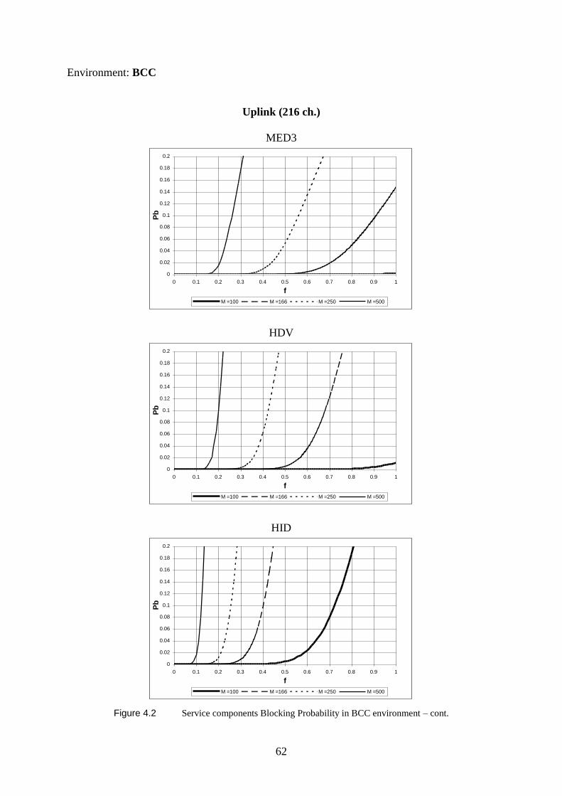
62
Environment: BCC
Uplink (216 ch.)
MED3
0
0.02
0.04
0.06
0.08
0.1
0.12
0.14
0.16
0.18
0.2
0 0.1 0.2 0.3 0.4 0.5 0.6 0.7 0.8 0.9 1
f
Pb
M =100 M =166 M =250 M =500
HDV
0
0.02
0.04
0.06
0.08
0.1
0.12
0.14
0.16
0.18
0.2
0 0.1 0.2 0.3 0.4 0.5 0.6 0.7 0.8 0.9 1
f
Pb
M =100 M =166 M =250 M =500
HID
0
0.02
0.04
0.06
0.08
0.1
0.12
0.14
0.16
0.18
0.2
0 0.1 0.2 0.3 0.4 0.5 0.6 0.7 0.8 0.9 1
f
Pb
M =100 M =166 M =250 M =500
Figure 4.2 Service components Blocking Probability in BCC environment – cont.
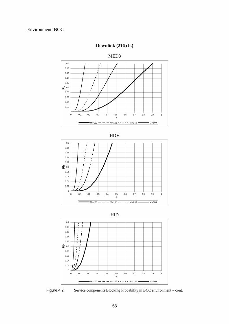
63
Environment: BCC
Downlink (216 ch.)
MED3
0
0.02
0.04
0.06
0.08
0.1
0.12
0.14
0.16
0.18
0.2
0 0.1 0.2 0.3 0.4 0.5 0.6 0.7 0.8 0.9 1
f
Pb
M =100 M =166 M =250 M =500
HDV
0
0.02
0.04
0.06
0.08
0.1
0.12
0.14
0.16
0.18
0.2
0 0.1 0.2 0.3 0.4 0.5 0.6 0.7 0.8 0.9 1
f
Pb
M =100 M =166 M =250 M =500
HID
0
0.02
0.04
0.06
0.08
0.1
0.12
0.14
0.16
0.18
0.2
0 0.1 0.2 0.3 0.4 0.5 0.6 0.7 0.8 0.9 1
f
Pb
M =100 M =166 M =250 M =500
Figure 4.2 Service components Blocking Probability in BCC environment – cont.
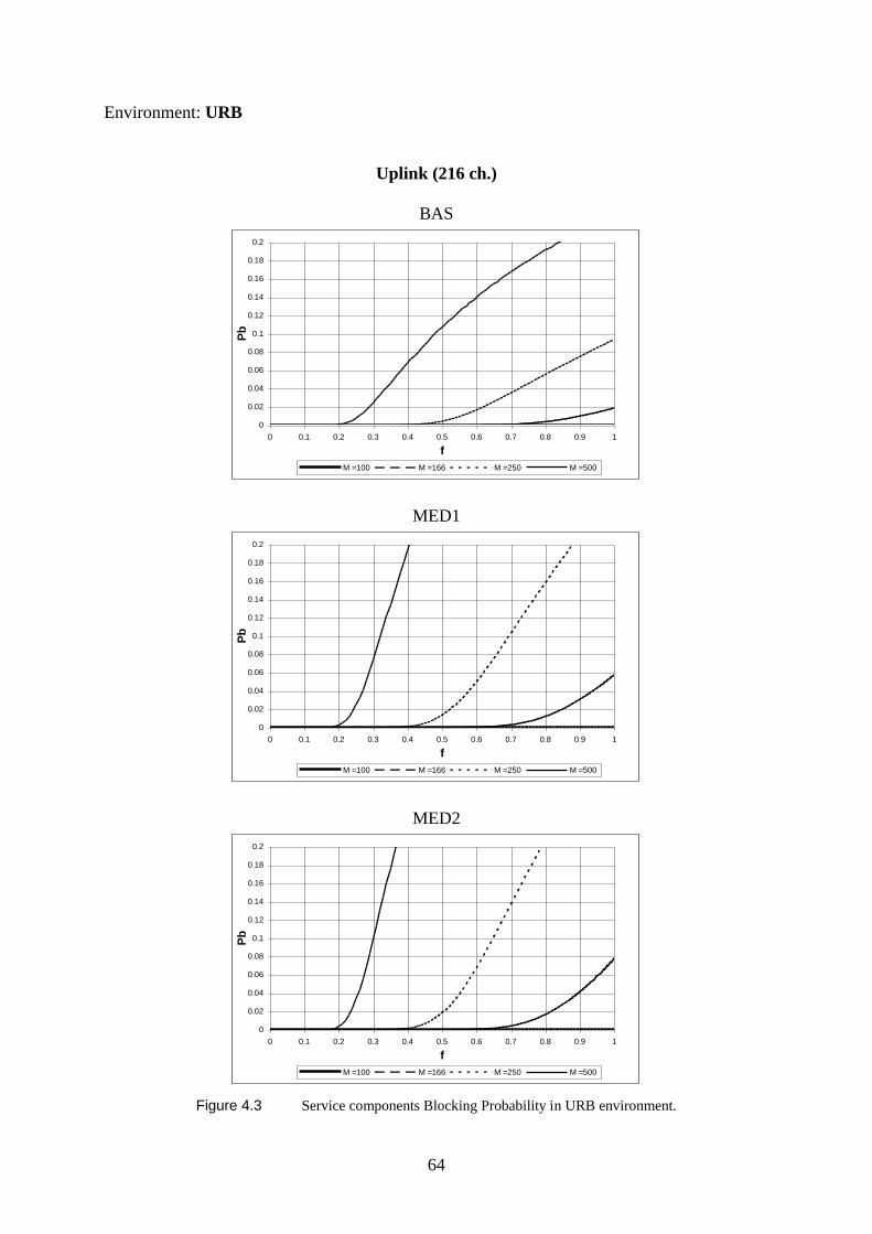
64
Environment: URB
Uplink (216 ch.)
BAS
0
0.02
0.04
0.06
0.08
0.1
0.12
0.14
0.16
0.18
0.2
0 0.1 0.2 0.3 0.4 0.5 0.6 0.7 0.8 0.9 1
f
Pb
M =100 M =166 M =250 M =500
MED1
0
0.02
0.04
0.06
0.08
0.1
0.12
0.14
0.16
0.18
0.2
0 0.1 0.2 0.3 0.4 0.5 0.6 0.7 0.8 0.9 1
f
Pb
M =100 M =166 M =250 M =500
MED2
0
0.02
0.04
0.06
0.08
0.1
0.12
0.14
0.16
0.18
0.2
0 0.1 0.2 0.3 0.4 0.5 0.6 0.7 0.8 0.9 1
f
Pb
M =100 M =166 M =250 M =500
Figure 4.3 Service components Blocking Probability in URB environment.

65
Environment: URB
Downlink (216 ch.)
BAS
0
0.02
0.04
0.06
0.08
0.1
0.12
0.14
0.16
0.18
0.2
0 0.1 0.2 0.3 0.4 0.5 0.6 0.7 0.8 0.9 1
f
Pb
M =100 M =166 M =250 M =500
MED1
0
0.02
0.04
0.06
0.08
0.1
0.12
0.14
0.16
0.18
0.2
0 0.1 0.2 0.3 0.4 0.5 0.6 0.7 0.8 0.9 1
f
Pb
M =100 M =166 M =250 M =500
MED2
0
0.02
0.04
0.06
0.08
0.1
0.12
0.14
0.16
0.18
0.2
0 0.1 0.2 0.3 0.4 0.5 0.6 0.7 0.8 0.9 1
f
Pb
M =100 M =166 M =250 M =500
Figure 4.3 Service components Blocking Probability in URB environment – cont.
66
Environment: URB
Uplink (216 ch.)
MED3
0
0.02
0.04
0.06
0.08
0.1
0.12
0.14
0.16
0.18
0.2
0 0.1 0.2 0.3 0.4 0.5 0.6 0.7 0.8 0.9 1
f
Pb
M =100 M =166 M =250 M =500
HDV
0
0.02
0.04
0.06
0.08
0.1
0.12
0.14
0.16
0.18
0.2
0 0.1 0.2 0.3 0.4 0.5 0.6 0.7 0.8 0.9 1
f
Pb
M =100 M =166 M =250 M =500
HID
0
0.02
0.04
0.06
0.08
0.1
0.12
0.14
0.16
0.18
0.2
0 0.1 0.2 0.3 0.4 0.5 0.6 0.7 0.8 0.9 1
f
Pb
M =100 M =166 M =250 M =500
Figure 4.3 Service components Blocking Probability in URB environment – cont.
67
Environment: URB
Downlink (216 ch.)
MED3
0
0.02
0.04
0.06
0.08
0.1
0.12
0.14
0.16
0.18
0.2
0 0.1 0.2 0.3 0.4 0.5 0.6 0.7 0.8 0.9 1
f
Pb
M =100 M =166 M =250 M =500
HDV
0
0.02
0.04
0.06
0.08
0.1
0.12
0.14
0.16
0.18
0.2
0 0.1 0.2 0.3 0.4 0.5 0.6 0.7 0.8 0.9 1
f
Pb
M =100 M =166 M =250 M =500
HID
0
0.02
0.04
0.06
0.08
0.1
0.12
0.14
0.16
0.18
0.2
0 0.1 0.2 0.3 0.4 0.5 0.6 0.7 0.8 0.9 1
f
Pb
M =100 M =166 M =250 M =500
Figure 4.3 Service components Blocking Probability in URB environment – cont.
68
Environment: ROA
Uplink (216 ch.)
BAS
0
0.02
0.04
0.06
0.08
0.1
0.12
0.14
0.16
0.18
0.2
0 0.1 0.2 0.3 0.4 0.5 0.6 0.7 0.8 0.9 1
f
Pb
M =100 M =166 M =250 M =500
MED1
0
0.02
0.04
0.06
0.08
0.1
0.12
0.14
0.16
0.18
0.2
0 0.1 0.2 0.3 0.4 0.5 0.6 0.7 0.8 0.9 1
f
Pb
M =100 M =166 M =250 M =500
MED2
0
0.02
0.04
0.06
0.08
0.1
0.12
0.14
0.16
0.18
0.2
0 0.1 0.2 0.3 0.4 0.5 0.6 0.7 0.8 0.9 1
f
Pb
M =100 M =166 M =250 M =500
Figure 4.4 Service components Blocking Probability in ROA environment.
69
Environment: ROA
Downlink (216 ch.)
BAS
0
0.02
0.04
0.06
0.08
0.1
0.12
0.14
0.16
0.18
0.2
0 0.1 0.2 0.3 0.4 0.5 0.6 0.7 0.8 0.9 1
f
Pb
M =100 M =166 M =250 M =500
MED1
0
0.02
0.04
0.06
0.08
0.1
0.12
0.14
0.16
0.18
0.2
0 0.1 0.2 0.3 0.4 0.5 0.6 0.7 0.8 0.9 1
f
Pb
M =100 M =166 M =250 M =500
MED2
0
0.02
0.04
0.06
0.08
0.1
0.12
0.14
0.16
0.18
0.2
0 0.1 0.2 0.3 0.4 0.5 0.6 0.7 0.8 0.9 1
f
Pb
M =100 M =166 M =250 M =500
Figure 4.4 Service components Blocking Probability in ROA environment – cont.
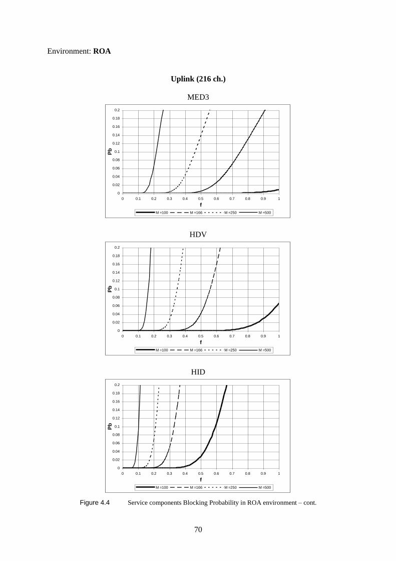
70
Environment: ROA
Uplink (216 ch.)
MED3
0
0.02
0.04
0.06
0.08
0.1
0.12
0.14
0.16
0.18
0.2
0 0.1 0.2 0.3 0.4 0.5 0.6 0.7 0.8 0.9 1
f
Pb
M =100 M =166 M =250 M =500
HDV
0
0.02
0.04
0.06
0.08
0.1
0.12
0.14
0.16
0.18
0.2
0 0.1 0.2 0.3 0.4 0.5 0.6 0.7 0.8 0.9 1
f
Pb
M =100 M =166 M =250 M =500
HID
0
0.02
0.04
0.06
0.08
0.1
0.12
0.14
0.16
0.18
0.2
0 0.1 0.2 0.3 0.4 0.5 0.6 0.7 0.8 0.9 1
f
Pb
M =100 M =166 M =250 M =500
Figure 4.4 Service components Blocking Probability in ROA environment – cont.
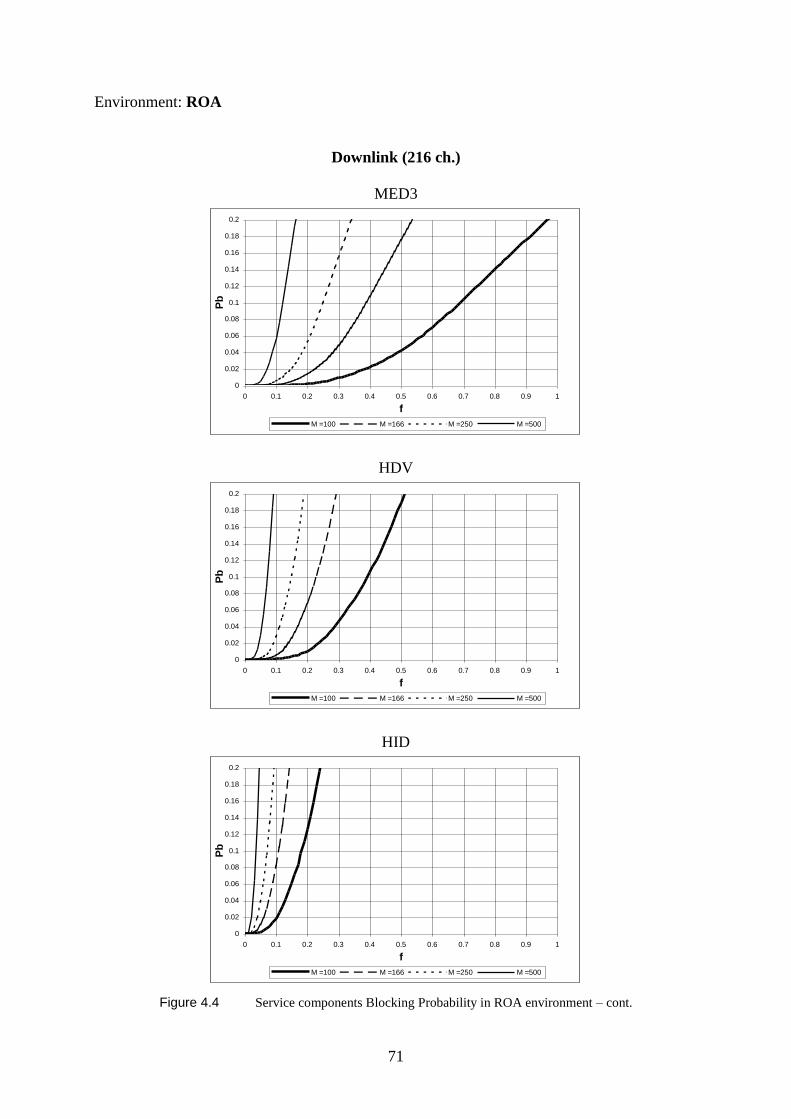
71
Environment: ROA
Downlink (216 ch.)
MED3
0
0.02
0.04
0.06
0.08
0.1
0.12
0.14
0.16
0.18
0.2
0 0.1 0.2 0.3 0.4 0.5 0.6 0.7 0.8 0.9 1
f
Pb
M =100 M =166 M =250 M =500
HDV
0
0.02
0.04
0.06
0.08
0.1
0.12
0.14
0.16
0.18
0.2
0 0.1 0.2 0.3 0.4 0.5 0.6 0.7 0.8 0.9 1
f
Pb
M =100 M =166 M =250 M =500
HID
0
0.02
0.04
0.06
0.08
0.1
0.12
0.14
0.16
0.18
0.2
0 0.1 0.2 0.3 0.4 0.5 0.6 0.7 0.8 0.9 1
f
Pb
M =100 M =166 M =250 M =500
Figure 4.4 Service components Blocking Probability in ROA environment – cont.
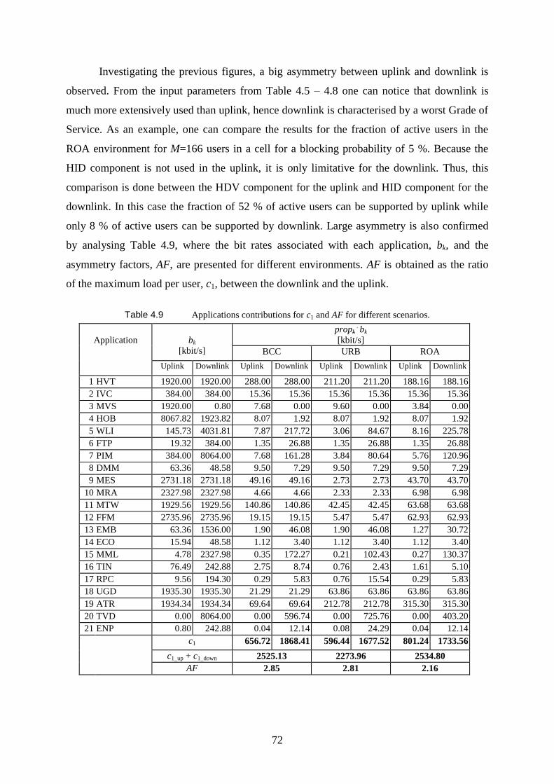
72
Investigating the previous figures, a big asymmetry between uplink and downlink is
observed. From the input parameters from Table 4.5 – 4.8 one can notice that downlink is
much more extensively used than uplink, hence downlink is characterised by a worst Grade of
Service. As an example, one can compare the results for the fraction of active users in the
ROA environment for M=166 users in a cell for a blocking probability of 5 %. Because the
HID component is not used in the uplink, it is only limitative for the downlink. Thus, this
comparison is done between the HDV component for the uplink and HID component for the
downlink. In this case the fraction of 52 % of active users can be supported by uplink while
only 8 % of active users can be supported by downlink. Large asymmetry is also confirmed
by analysing Table 4.9, where the bit rates associated with each application, bk, and the
asymmetry factors, AF, are presented for different environments. AF is obtained as the ratio
of the maximum load per user, c1, between the downlink and the uplink.
Table 4.9 Applications contributions for c1 and AF for different scenarios.
Application
bk
[kbit/s]
propk . bk
[kbit/s]
BCC URB ROA
Uplink Downlink Uplink Downlink Uplink Downlink Uplink Downlink
1 HVT 1920.00 1920.00 288.00 288.00 211.20 211.20 188.16 188.16
2 IVC 384.00 384.00 15.36 15.36 15.36 15.36 15.36 15.36
3 MVS 1920.00 0.80 7.68 0.00 9.60 0.00 3.84 0.00
4 HOB 8067.82 1923.82 8.07 1.92 8.07 1.92 8.07 1.92
5 WLI 145.73 4031.81 7.87 217.72 3.06 84.67 8.16 225.78
6 FTP 19.32 384.00 1.35 26.88 1.35 26.88 1.35 26.88
7 PIM 384.00 8064.00 7.68 161.28 3.84 80.64 5.76 120.96
8 DMM 63.36 48.58 9.50 7.29 9.50 7.29 9.50 7.29
9 MES 2731.18 2731.18 49.16 49.16 2.73 2.73 43.70 43.70
10 MRA 2327.98 2327.98 4.66 4.66 2.33 2.33 6.98 6.98
11 MTW 1929.56 1929.56 140.86 140.86 42.45 42.45 63.68 63.68
12 FFM 2735.96 2735.96 19.15 19.15 5.47 5.47 62.93 62.93
13 EMB 63.36 1536.00 1.90 46.08 1.90 46.08 1.27 30.72
14 ECO 15.94 48.58 1.12 3.40 1.12 3.40 1.12 3.40
15 MML 4.78 2327.98 0.35 172.27 0.21 102.43 0.27 130.37
16 TIN 76.49 242.88 2.75 8.74 0.76 2.43 1.61 5.10
17 RPC 9.56 194.30 0.29 5.83 0.76 15.54 0.29 5.83
18 UGD 1935.30 1935.30 21.29 21.29 63.86 63.86 63.86 63.86
19 ATR 1934.34 1934.34 69.64 69.64 212.78 212.78 315.30 315.30
20 TVD 0.00 8064.00 0.00 596.74 0.00 725.76 0.00 403.20
21 ENP 0.80 242.88 0.04 12.14 0.08 24.29 0.04 12.14
c1 656.72 1868.41 596.44 1677.52 801.24 1733.56
c1_up + c1_down 2525.13 2273.96 2534.80
AF 2.85 2.81 2.16
73
Using asymmetry factors one can use the following formula for the channels in order to
obtain a better balance between uplink and downlink for a service components:
AF
AF
AF
totaldownlink
totaluplink
CC
CC
1
1 (4.1)
After some simulations another set of equations seems to be a better approach:
uplinktotaldownlink
totaluplink
CCC
CC
.AF%x
.AF x x
AF 02for 1582for 0
(4.2)
The numbers used for TDD mode simulations are presented in Table 4.10. It is
important to remark that still the same scenario is considered but now channels from uplink
and downlink are merged which leads to a pool of 432 user channels available for the system.
Table 4.10 Number of channels used for TDD mode analysis.
Environment Number of channels
dedicated for Uplink
Number of channels
dedicated for Downlink
BCC 152 280
URB 154 278
ROA 170 262
Figure 4.5 – 4.7 present the results obtained according to the new number of channels in TDD
mode i.e., the case where asymmetry can be supported (152 channels for uplink and 280 for
channels for downlink). It is important to remark that the same assumptions and input
parameters than in FDD mode are kept to find a more efficient solution by direct comparison.
74
Environment: BCC
Uplink (152 ch.)
BAS
0
0.02
0.04
0.06
0.08
0.1
0.12
0.14
0.16
0.18
0.2
0 0.1 0.2 0.3 0.4 0.5 0.6 0.7 0.8 0.9 1
f
Pb
M =100 M =166 M =250 M =500
MED1
0
0.02
0.04
0.06
0.08
0.1
0.12
0.14
0.16
0.18
0.2
0 0.1 0.2 0.3 0.4 0.5 0.6 0.7 0.8 0.9 1
f
Pb
M =100 M =166 M =250 M =500
MED2
0
0.02
0.04
0.06
0.08
0.1
0.12
0.14
0.16
0.18
0.2
0 0.1 0.2 0.3 0.4 0.5 0.6 0.7 0.8 0.9 1
f
Pb
M =100 M =166 M =250 M =500
Figure 4.5 Service components Blocking Probability in BCC environment for TDD Mode.
75
Environment: BCC
Downlink (280 ch.)
BAS
0
0.02
0.04
0.06
0.08
0.1
0.12
0.14
0.16
0.18
0.2
0 0.1 0.2 0.3 0.4 0.5 0.6 0.7 0.8 0.9 1
f
Pb
M =100 M =166 M =250 M =500
MED1
0
0.02
0.04
0.06
0.08
0.1
0.12
0.14
0.16
0.18
0.2
0 0.1 0.2 0.3 0.4 0.5 0.6 0.7 0.8 0.9 1
f
Pb
M =100 M =166 M =250 M =500
MED2
0
0.02
0.04
0.06
0.08
0.1
0.12
0.14
0.16
0.18
0.2
0 0.1 0.2 0.3 0.4 0.5 0.6 0.7 0.8 0.9 1
f
Pb
M =100 M =166 M =250 M =500
Figure 4.5 Service components Blocking Probability in BCC environment for TDD Mode – cont.
76
Environment: BCC
Uplink (152 ch.)
MED3
0
0.02
0.04
0.06
0.08
0.1
0.12
0.14
0.16
0.18
0.2
0 0.1 0.2 0.3 0.4 0.5 0.6 0.7 0.8 0.9 1
f
Pb
M =100 M =166 M =250 M =500
HDV
0
0.02
0.04
0.06
0.08
0.1
0.12
0.14
0.16
0.18
0.2
0 0.1 0.2 0.3 0.4 0.5 0.6 0.7 0.8 0.9 1
f
Pb
M =100 M =166 M =250 M =500
HID
0
0.02
0.04
0.06
0.08
0.1
0.12
0.14
0.16
0.18
0.2
0 0.1 0.2 0.3 0.4 0.5 0.6 0.7 0.8 0.9 1
f
Pb
M =100 M =166 M =250 M =500
Figure 4.5 Service components Blocking Probability in BCC environment for TDD Mode – cont.
77
Environment: BCC
Downlink (280 ch.)
MED3
0
0.02
0.04
0.06
0.08
0.1
0.12
0.14
0.16
0.18
0.2
0 0.1 0.2 0.3 0.4 0.5 0.6 0.7 0.8 0.9 1
f
Pb
M =100 M =166 M =250 M =500
HDV
0
0.02
0.04
0.06
0.08
0.1
0.12
0.14
0.16
0.18
0.2
0 0.1 0.2 0.3 0.4 0.5 0.6 0.7 0.8 0.9 1
f
Pb
M =100 M =166 M =250 M =500
HID
0
0.02
0.04
0.06
0.08
0.1
0.12
0.14
0.16
0.18
0.2
0 0.1 0.2 0.3 0.4 0.5 0.6 0.7 0.8 0.9 1
f
Pb
M =100 M =166 M =250 M =500
Figure 4.5 Service components Blocking Probability in BCC environment for TDD Mode – cont.
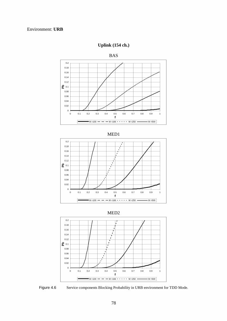
78
Environment: URB
Uplink (154 ch.)
BAS
0
0.02
0.04
0.06
0.08
0.1
0.12
0.14
0.16
0.18
0.2
0 0.1 0.2 0.3 0.4 0.5 0.6 0.7 0.8 0.9 1
f
Pb
M =100 M =166 M =250 M =500
MED1
0
0.02
0.04
0.06
0.08
0.1
0.12
0.14
0.16
0.18
0.2
0 0.1 0.2 0.3 0.4 0.5 0.6 0.7 0.8 0.9 1
f
Pb
M =100 M =166 M =250 M =500
MED2
0
0.02
0.04
0.06
0.08
0.1
0.12
0.14
0.16
0.18
0.2
0 0.1 0.2 0.3 0.4 0.5 0.6 0.7 0.8 0.9 1
f
Pb
M =100 M =166 M =250 M =500
Figure 4.6 Service components Blocking Probability in URB environment for TDD Mode.
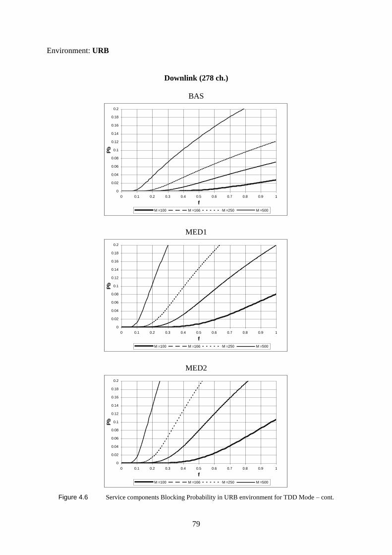
79
Environment: URB
Downlink (278 ch.)
BAS
0
0.02
0.04
0.06
0.08
0.1
0.12
0.14
0.16
0.18
0.2
0 0.1 0.2 0.3 0.4 0.5 0.6 0.7 0.8 0.9 1
f
Pb
M =100 M =166 M =250 M =500
MED1
0
0.02
0.04
0.06
0.08
0.1
0.12
0.14
0.16
0.18
0.2
0 0.1 0.2 0.3 0.4 0.5 0.6 0.7 0.8 0.9 1
f
Pb
M =100 M =166 M =250 M =500
MED2
0
0.02
0.04
0.06
0.08
0.1
0.12
0.14
0.16
0.18
0.2
0 0.1 0.2 0.3 0.4 0.5 0.6 0.7 0.8 0.9 1
f
Pb
M =100 M =166 M =250 M =500
Figure 4.6 Service components Blocking Probability in URB environment for TDD Mode – cont.
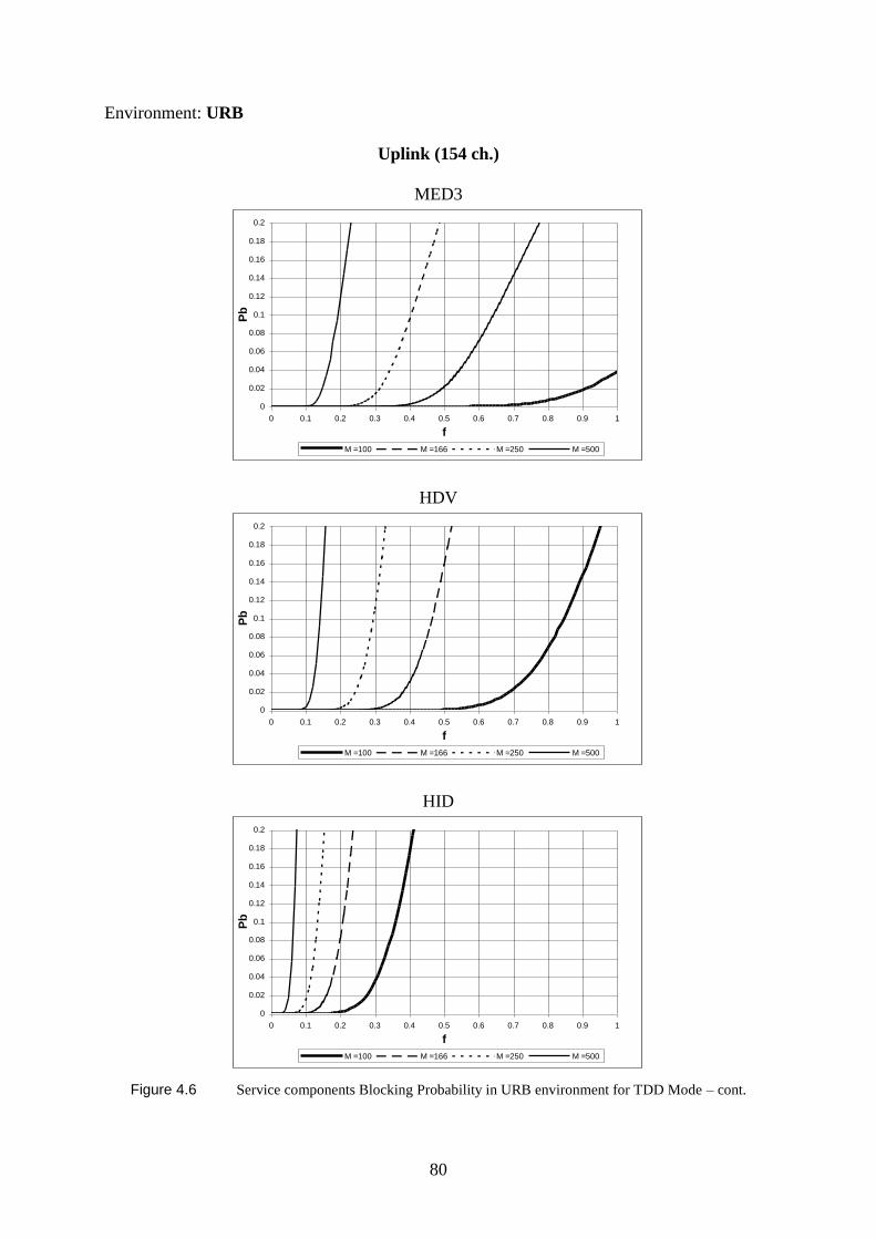
80
Environment: URB
Uplink (154 ch.)
MED3
0
0.02
0.04
0.06
0.08
0.1
0.12
0.14
0.16
0.18
0.2
0 0.1 0.2 0.3 0.4 0.5 0.6 0.7 0.8 0.9 1
f
Pb
M =100 M =166 M =250 M =500
HDV
0
0.02
0.04
0.06
0.08
0.1
0.12
0.14
0.16
0.18
0.2
0 0.1 0.2 0.3 0.4 0.5 0.6 0.7 0.8 0.9 1
f
Pb
M =100 M =166 M =250 M =500
HID
0
0.02
0.04
0.06
0.08
0.1
0.12
0.14
0.16
0.18
0.2
0 0.1 0.2 0.3 0.4 0.5 0.6 0.7 0.8 0.9 1
f
Pb
M =100 M =166 M =250 M =500
Figure 4.6 Service components Blocking Probability in URB environment for TDD Mode – cont.
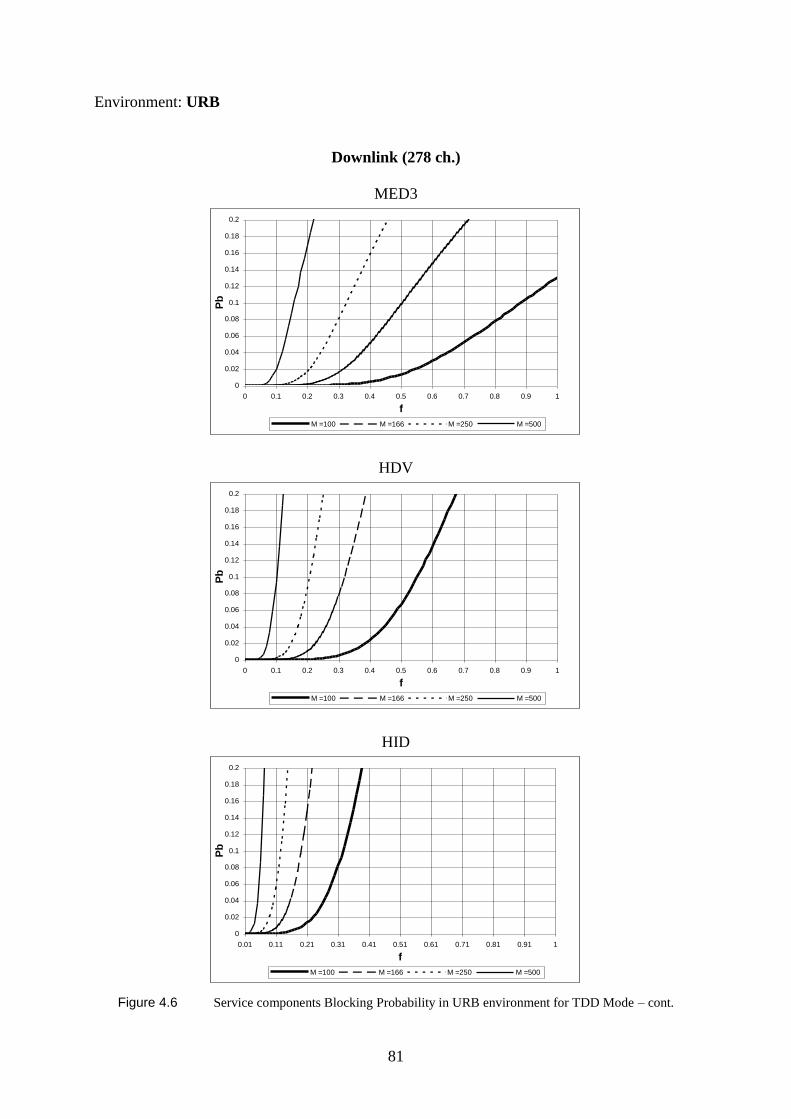
81
Environment: URB
Downlink (278 ch.)
MED3
0
0.02
0.04
0.06
0.08
0.1
0.12
0.14
0.16
0.18
0.2
0 0.1 0.2 0.3 0.4 0.5 0.6 0.7 0.8 0.9 1
f
Pb
M =100 M =166 M =250 M =500
HDV
0
0.02
0.04
0.06
0.08
0.1
0.12
0.14
0.16
0.18
0.2
0 0.1 0.2 0.3 0.4 0.5 0.6 0.7 0.8 0.9 1
f
Pb
M =100 M =166 M =250 M =500
HID
0
0.02
0.04
0.06
0.08
0.1
0.12
0.14
0.16
0.18
0.2
0.01 0.11 0.21 0.31 0.41 0.51 0.61 0.71 0.81 0.91 1
f
Pb
M =100 M =166 M =250 M =500
Figure 4.6 Service components Blocking Probability in URB environment for TDD Mode – cont.
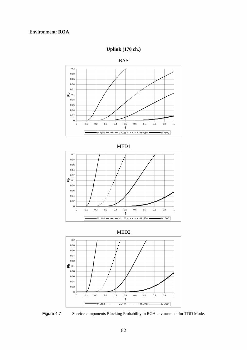
82
Environment: ROA
Uplink (170 ch.)
BAS
0
0.02
0.04
0.06
0.08
0.1
0.12
0.14
0.16
0.18
0.2
0 0.1 0.2 0.3 0.4 0.5 0.6 0.7 0.8 0.9 1
f
Pb
M =100 M =166 M =250 M =500
MED1
0
0.02
0.04
0.06
0.08
0.1
0.12
0.14
0.16
0.18
0.2
0 0.1 0.2 0.3 0.4 0.5 0.6 0.7 0.8 0.9 1
f
Pb
M =100 M =166 M =250 M =500
MED2
0
0.02
0.04
0.06
0.08
0.1
0.12
0.14
0.16
0.18
0.2
0 0.1 0.2 0.3 0.4 0.5 0.6 0.7 0.8 0.9 1
f
Pb
M =100 M =166 M =250 M =500
Figure 4.7 Service components Blocking Probability in ROA environment for TDD Mode.
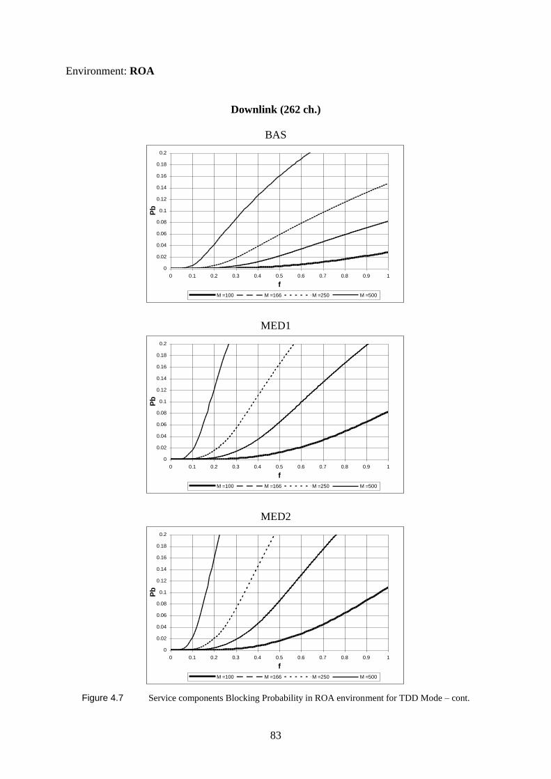
83
Environment: ROA
Downlink (262 ch.)
BAS
0
0.02
0.04
0.06
0.08
0.1
0.12
0.14
0.16
0.18
0.2
0 0.1 0.2 0.3 0.4 0.5 0.6 0.7 0.8 0.9 1
f
Pb
M =100 M =166 M =250 M =500
MED1
0
0.02
0.04
0.06
0.08
0.1
0.12
0.14
0.16
0.18
0.2
0 0.1 0.2 0.3 0.4 0.5 0.6 0.7 0.8 0.9 1
f
Pb
M =100 M =166 M =250 M =500
MED2
0
0.02
0.04
0.06
0.08
0.1
0.12
0.14
0.16
0.18
0.2
0 0.1 0.2 0.3 0.4 0.5 0.6 0.7 0.8 0.9 1
f
Pb
M =100 M =166 M =250 M =500
Figure 4.7 Service components Blocking Probability in ROA environment for TDD Mode – cont.
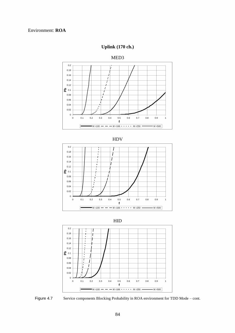
84
Environment: ROA
Uplink (170 ch.)
MED3
0
0.02
0.04
0.06
0.08
0.1
0.12
0.14
0.16
0.18
0.2
0 0.1 0.2 0.3 0.4 0.5 0.6 0.7 0.8 0.9 1
f
Pb
M =100 M =166 M =250 M =500
HDV
0
0.02
0.04
0.06
0.08
0.1
0.12
0.14
0.16
0.18
0.2
0 0.1 0.2 0.3 0.4 0.5 0.6 0.7 0.8 0.9 1
f
Pb
M =100 M =166 M =250 M =500
HID
0
0.02
0.04
0.06
0.08
0.1
0.12
0.14
0.16
0.18
0.2
0 0.1 0.2 0.3 0.4 0.5 0.6 0.7 0.8 0.9 1
f
Pb
M =100 M =166 M =250 M =500
Figure 4.7 Service components Blocking Probability in ROA environment for TDD Mode – cont.
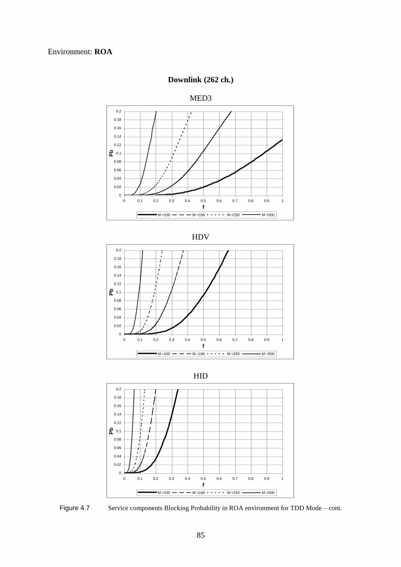
85
Environment: ROA
Downlink (262 ch.)
MED3
0
0.02
0.04
0.06
0.08
0.1
0.12
0.14
0.16
0.18
0.2
0 0.1 0.2 0.3 0.4 0.5 0.6 0.7 0.8 0.9 1
f
Pb
M =100 M =166 M =250 M =500
HDV
0
0.02
0.04
0.06
0.08
0.1
0.12
0.14
0.16
0.18
0.2
0 0.1 0.2 0.3 0.4 0.5 0.6 0.7 0.8 0.9 1
f
Pb
M =100 M =166 M =250 M =500
HID
0
0.02
0.04
0.06
0.08
0.1
0.12
0.14
0.16
0.18
0.2
0 0.1 0.2 0.3 0.4 0.5 0.6 0.7 0.8 0.9 1
f
Pb
M =100 M =166 M =250 M =500
Figure 4.7 Service components Blocking Probability in ROA environment for TDD Mode – cont.
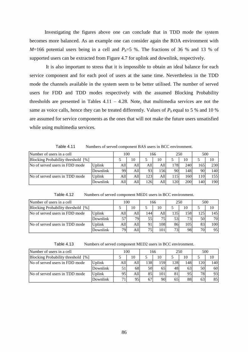
86
Investigating the figures above one can conclude that in TDD mode the system
becomes more balanced. As an example one can consider again the ROA environment with
M=166 potential users being in a cell and Pb=5 %. The fractions of 36 % and 13 % of
supported users can be extracted from Figure 4.7 for uplink and downlink, respectively.
It is also important to stress that it is impossible to obtain an ideal balance for each
service component and for each pool of users at the same time. Nevertheless in the TDD
mode the channels available in the system seem to be better utilised. The number of served
users for FDD and TDD modes respectively with the assumed Blocking Probability
thresholds are presented in Tables 4.11 – 4.28. Note, that multimedia services are not the
same as voice calls, hence they can be treated differently. Values of Pb equal to 5 % and 10 %
are assumed for service components as the ones that will not make the future users unsatisfied
while using multimedia services.
Table 4.11 Numbers of served component BAS users in BCC environment.
Number of users in a cell 100 166 250 500
Blocking Probability threshold [%] 5 10 5 10 5 10 5 10
No of served users in FDD mode Uplink All All All All 178 240 165 230
Downlink 99 All 93 156 90 148 90 140
No of served users in TDD mode Uplink All All 123 All 115 160 110 155
Downlink All All 126 All 120 200 140 190
Table 4.12 Numbers of served component MED1 users in BCC environment.
Number of users in a cell 100 166 250 500
Blocking Probability threshold [%] 5 10 5 10 5 10 5 10
No of served users in FDD mode Uplink All All 144 All 135 158 125 145
Downlink 57 79 55 75 53 73 50 70
No of served users in TDD mode Uplink All All 91 108 86 105 83 100
Downlink 79 All 75 101 73 98 70 95
Table 4.13 Numbers of served component MED2 users in BCC environment.
Number of users in a cell 100 166 250 500
Blocking Probability threshold [%] 5 10 5 10 5 10 5 10
No of served users in FDD mode Uplink All All 138 159 128 148 120 140
Downlink 51 68 50 65 48 63 50 60
No of served users in TDD mode Uplink 95 All 85 101 81 95 78 93
Downlink 71 95 67 90 65 88 63 85
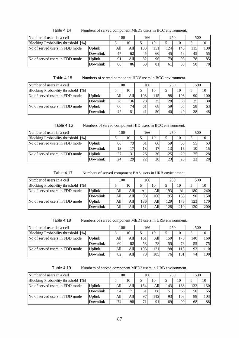
87
Table 4.14 Numbers of served component MED3 users in BCC environment.
Number of users in a cell 100 166 250 500
Blocking Probability threshold [%] 5 10 5 10 5 10 5 10
No of served users in FDD mode Uplink All All 133 151 124 140 115 130
Downlink 47 62 45 60 45 58 45 55
No of served users in TDD mode Uplink 91 All 82 96 79 93 78 85
Downlink 66 86 63 81 61 80 58 78
Table 4.15 Numbers of served component HDV users in BCC environment.
Number of users in a cell 100 166 250 500
Blocking Probability threshold [%] 5 10 5 10 5 10 5 10
No of served users in FDD mode Uplink All All 103 115 98 108 90 100
Downlink 28 36 28 35 28 35 25 30
No of served users in TDD mode Uplink 66 74 61 68 59 65 58 63
Downlink 42 51 41 50 40 49 38 48
Table 4.16 Numbers of served component HID users in BCC environment.
Number of users in a cell 100 166 250 500
Blocking Probability threshold [%] 5 10 5 10 5 10 5 10
No of served users in FDD mode Uplink 66 73 61 66 59 65 55 63
Downlink 13 17 13 17 13 15 10 15
No of served users in TDD mode Uplink 27 31 26 30 25 29 25 28
Downlink 24 29 22 28 23 28 22 28
Table 4.17 Numbers of served component BAS users in URB environment.
Number of users in a cell 100 166 250 500
Blocking Probability threshold [%] 5 10 5 10 5 10 5 10
No of served users in FDD mode Uplink All All All All 193 All 180 240
Downlink All All 98 166 95 158 90 150
No of served users in TDD mode Uplink All All 136 All 129 175 123 170
Downlink All All 131 All 128 210 120 200
Table 4.18 Numbers of served component MED1 users in URB environment.
Number of users in a cell 100 166 250 500
Blocking Probability threshold [%] 5 10 5 10 5 10 5 10
No of served users in FDD mode Uplink All All 161 All 150 175 140 160
Downlink 60 82 58 78 55 78 55 75
No of served users in TDD mode Uplink All All 103 121 98 115 93 110
Downlink 82 All 78 105 76 101 74 100
Table 4.19 Numbers of served component MED2 users in URB environment.
Number of users in a cell 100 166 250 500
Blocking Probability threshold [%] 5 10 5 10 5 10 5 10
No of served users in FDD mode Uplink All All 154 All 143 163 133 150
Downlink 54 71 51 68 51 68 50 65
No of served users in TDD mode Uplink All All 97 112 93 108 88 103
Downlink 74 98 71 91 69 90 68 88
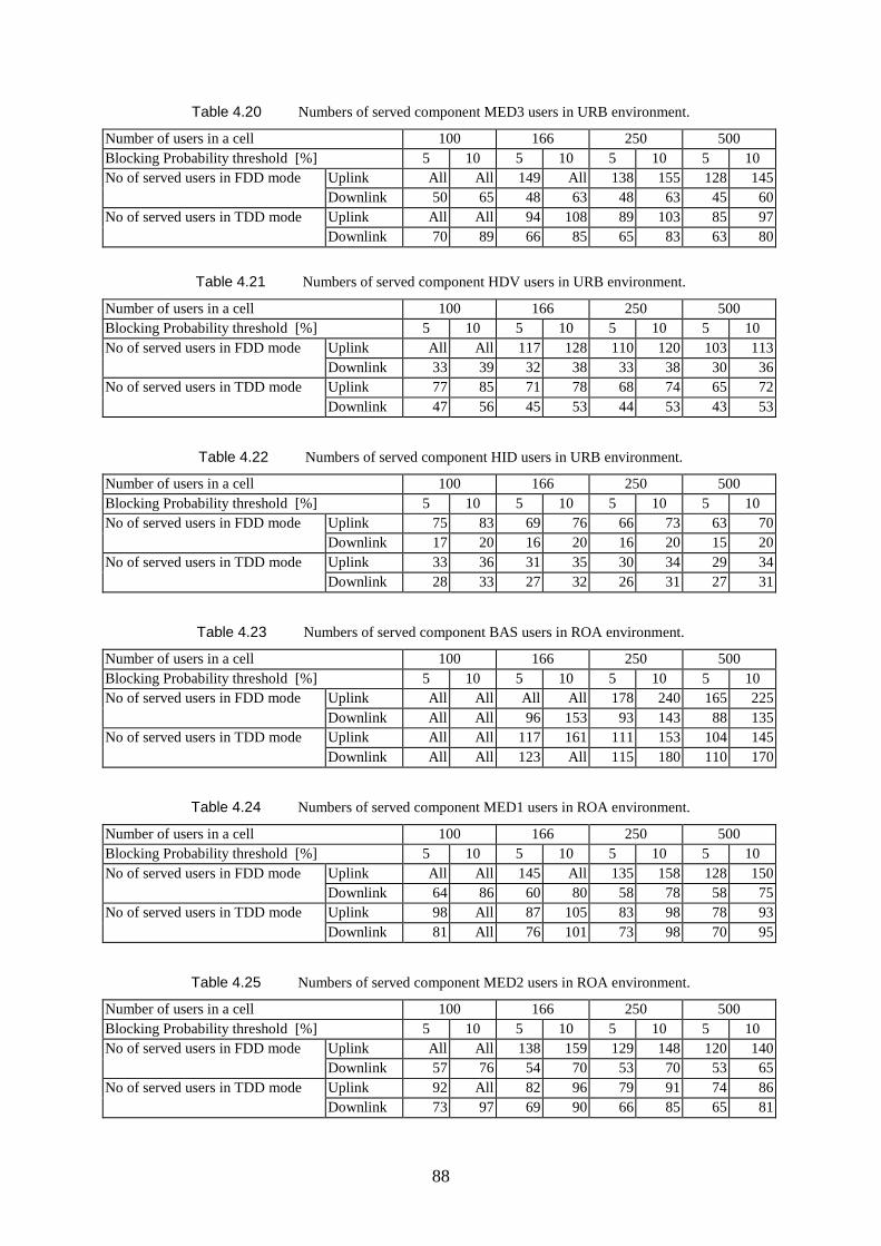
88
Table 4.20 Numbers of served component MED3 users in URB environment.
Number of users in a cell 100 166 250 500
Blocking Probability threshold [%] 5 10 5 10 5 10 5 10
No of served users in FDD mode Uplink All All 149 All 138 155 128 145
Downlink 50 65 48 63 48 63 45 60
No of served users in TDD mode Uplink All All 94 108 89 103 85 97
Downlink 70 89 66 85 65 83 63 80
Table 4.21 Numbers of served component HDV users in URB environment.
Number of users in a cell 100 166 250 500
Blocking Probability threshold [%] 5 10 5 10 5 10 5 10
No of served users in FDD mode Uplink All All 117 128 110 120 103 113
Downlink 33 39 32 38 33 38 30 36
No of served users in TDD mode Uplink 77 85 71 78 68 74 65 72
Downlink 47 56 45 53 44 53 43 53
Table 4.22 Numbers of served component HID users in URB environment.
Number of users in a cell 100 166 250 500
Blocking Probability threshold [%] 5 10 5 10 5 10 5 10
No of served users in FDD mode Uplink 75 83 69 76 66 73 63 70
Downlink 17 20 16 20 16 20 15 20
No of served users in TDD mode Uplink 33 36 31 35 30 34 29 34
Downlink 28 33 27 32 26 31 27 31
Table 4.23 Numbers of served component BAS users in ROA environment.
Number of users in a cell 100 166 250 500
Blocking Probability threshold [%] 5 10 5 10 5 10 5 10
No of served users in FDD mode Uplink All All All All 178 240 165 225
Downlink All All 96 153 93 143 88 135
No of served users in TDD mode Uplink All All 117 161 111 153 104 145
Downlink All All 123 All 115 180 110 170
Table 4.24 Numbers of served component MED1 users in ROA environment.
Number of users in a cell 100 166 250 500
Blocking Probability threshold [%] 5 10 5 10 5 10 5 10
No of served users in FDD mode Uplink All All 145 All 135 158 128 150
Downlink 64 86 60 80 58 78 58 75
No of served users in TDD mode Uplink 98 All 87 105 83 98 78 93
Downlink 81 All 76 101 73 98 70 95
Table 4.25 Numbers of served component MED2 users in ROA environment.
Number of users in a cell 100 166 250 500
Blocking Probability threshold [%] 5 10 5 10 5 10 5 10
No of served users in FDD mode Uplink All All 138 159 129 148 120 140
Downlink 57 76 54 70 53 70 53 65
No of served users in TDD mode Uplink 92 All 82 96 79 91 74 86
Downlink 73 97 69 90 66 85 65 81
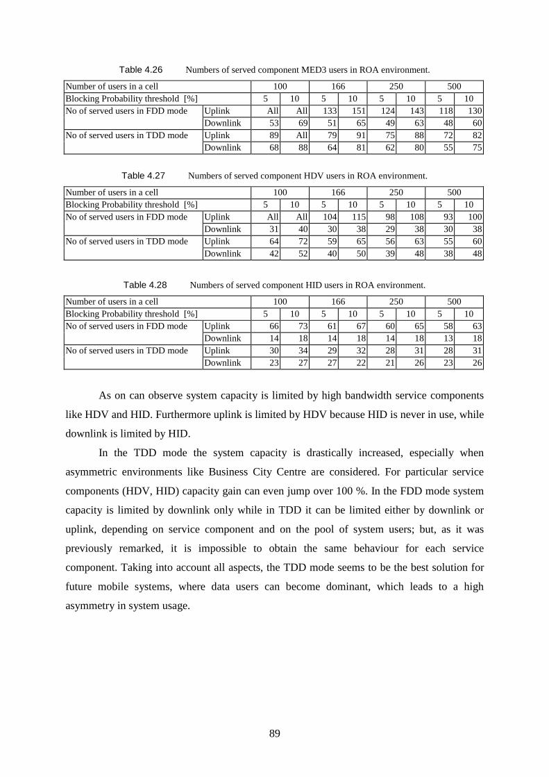
89
Table 4.26 Numbers of served component MED3 users in ROA environment.
Number of users in a cell 100 166 250 500
Blocking Probability threshold [%] 5 10 5 10 5 10 5 10
No of served users in FDD mode Uplink All All 133 151 124 143 118 130
Downlink 53 69 51 65 49 63 48 60
No of served users in TDD mode Uplink 89 All 79 91 75 88 72 82
Downlink 68 88 64 81 62 80 55 75
Table 4.27 Numbers of served component HDV users in ROA environment.
Number of users in a cell 100 166 250 500
Blocking Probability threshold [%] 5 10 5 10 5 10 5 10
No of served users in FDD mode Uplink All All 104 115 98 108 93 100
Downlink 31 40 30 38 29 38 30 38
No of served users in TDD mode Uplink 64 72 59 65 56 63 55 60
Downlink 42 52 40 50 39 48 38 48
Table 4.28 Numbers of served component HID users in ROA environment.
Number of users in a cell 100 166 250 500
Blocking Probability threshold [%] 5 10 5 10 5 10 5 10
No of served users in FDD mode Uplink 66 73 61 67 60 65 58 63
Downlink 14 18 14 18 14 18 13 18
No of served users in TDD mode Uplink 30 34 29 32 28 31 28 31
Downlink 23 27 27 22 21 26 23 26
As on can observe system capacity is limited by high bandwidth service components
like HDV and HID. Furthermore uplink is limited by HDV because HID is never in use, while
downlink is limited by HID.
In the TDD mode the system capacity is drastically increased, especially when
asymmetric environments like Business City Centre are considered. For particular service
components (HDV, HID) capacity gain can even jump over 100 %. In the FDD mode system
capacity is limited by downlink only while in TDD it can be limited either by downlink or
uplink, depending on service component and on the pool of system users; but, as it was
previously remarked, it is impossible to obtain the same behaviour for each service
component. Taking into account all aspects, the TDD mode seems to be the best solution for
future mobile systems, where data users can become dominant, which leads to a high
asymmetry in system usage.
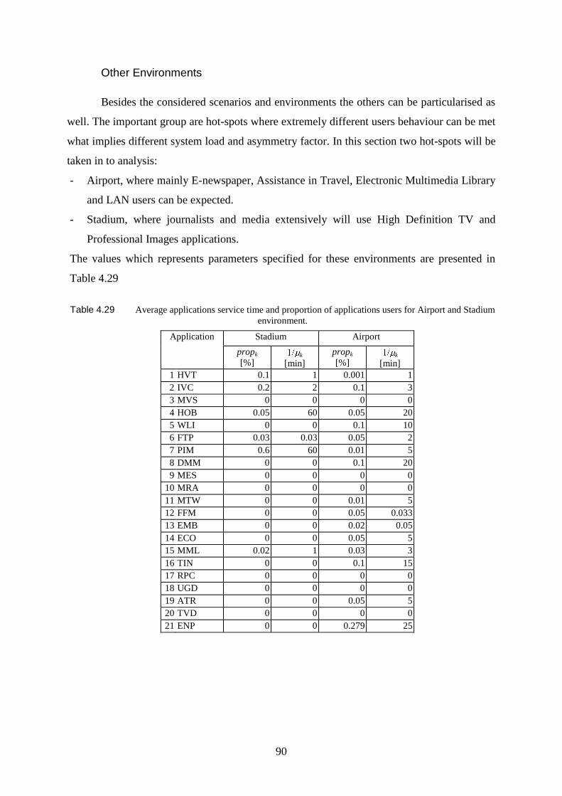
90
Other Environments
Besides the considered scenarios and environments the others can be particularised as
well. The important group are hot-spots where extremely different users behaviour can be met
what implies different system load and asymmetry factor. In this section two hot-spots will be
taken in to analysis:
- Airport, where mainly E-newspaper, Assistance in Travel, Electronic Multimedia Library
and LAN users can be expected.
- Stadium, where journalists and media extensively will use High Definition TV and
Professional Images applications.
The values which represents parameters specified for these environments are presented in
Table 4.29
Table 4.29 Average applications service time and proportion of applications users for Airport and Stadium
environment.
Application Stadium Airport
propk
[%] k
[min]
propk
[%] k
[min]
1 HVT 0.1 1 0.001 1
2 IVC 0.2 2 0.1 3
3 MVS 0 0 0 0
4 HOB 0.05 60 0.05 20
5 WLI 0 0 0.1 10
6 FTP 0.03 0.03 0.05 2
7 PIM 0.6 60 0.01 5
8 DMM 0 0 0.1 20
9 MES 0 0 0 0
10 MRA 0 0 0 0
11 MTW 0 0 0.01 5
12 FFM 0 0 0.05 0.033
13 EMB 0 0 0.02 0.05
14 ECO 0 0 0.05 5
15 MML 0.02 1 0.03 3
16 TIN 0 0 0.1 15
17 RPC 0 0 0 0
18 UGD 0 0 0 0
19 ATR 0 0 0.05 5
20 TVD 0 0 0 0
21 ENP 0 0 0.279 25
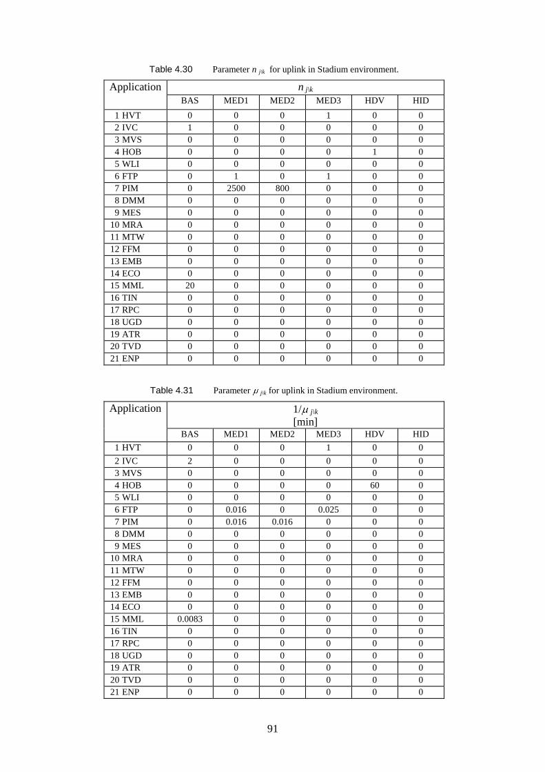
91
Table 4.30 Parameter n j\k for uplink in Stadium environment.
Application n j\k
BAS MED1 MED2 MED3 HDV HID
1 HVT 0 0 0 1 0 0
2 IVC 1 0 0 0 0 0
3 MVS 0 0 0 0 0 0
4 HOB 0 0 0 0 1 0
5 WLI 0 0 0 0 0 0
6 FTP 0 1 0 1 0 0
7 PIM 0 2500 800 0 0 0
8 DMM 0 0 0 0 0 0
9 MES 0 0 0 0 0 0
10 MRA 0 0 0 0 0 0
11 MTW 0 0 0 0 0 0
12 FFM 0 0 0 0 0 0
13 EMB 0 0 0 0 0 0
14 ECO 0 0 0 0 0 0
15 MML 20 0 0 0 0 0
16 TIN 0 0 0 0 0 0
17 RPC 0 0 0 0 0 0
18 UGD 0 0 0 0 0 0
19 ATR 0 0 0 0 0 0
20 TVD 0 0 0 0 0 0
21 ENP 0 0 0 0 0 0
Table 4.31 Parameter j\k for uplink in Stadium environment.
Application 1/ j\k
[min] BAS MED1 MED2 MED3 HDV HID
1 HVT 0 0 0 1 0 0
2 IVC 2 0 0 0 0 0
3 MVS 0 0 0 0 0 0
4 HOB 0 0 0 0 60 0
5 WLI 0 0 0 0 0 0
6 FTP 0 0.016 0 0.025 0 0
7 PIM 0 0.016 0.016 0 0 0
8 DMM 0 0 0 0 0 0
9 MES 0 0 0 0 0 0
10 MRA 0 0 0 0 0 0
11 MTW 0 0 0 0 0 0
12 FFM 0 0 0 0 0 0
13 EMB 0 0 0 0 0 0
14 ECO 0 0 0 0 0 0
15 MML 0.0083 0 0 0 0 0
16 TIN 0 0 0 0 0 0
17 RPC 0 0 0 0 0 0
18 UGD 0 0 0 0 0 0
19 ATR 0 0 0 0 0 0
20 TVD 0 0 0 0 0 0
21 ENP 0 0 0 0 0 0
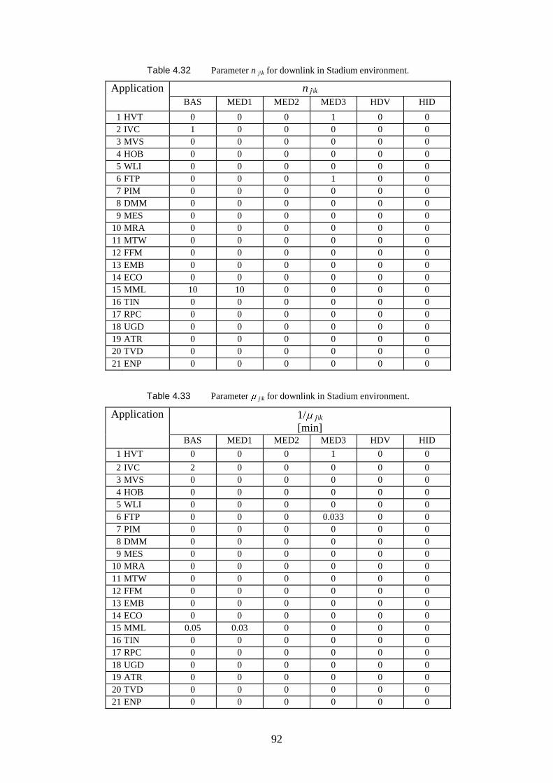
92
Table 4.32 Parameter n j\k for downlink in Stadium environment.
Application n j\k
BAS MED1 MED2 MED3 HDV HID
1 HVT 0 0 0 1 0 0
2 IVC 1 0 0 0 0 0
3 MVS 0 0 0 0 0 0
4 HOB 0 0 0 0 0 0
5 WLI 0 0 0 0 0 0
6 FTP 0 0 0 1 0 0
7 PIM 0 0 0 0 0 0
8 DMM 0 0 0 0 0 0
9 MES 0 0 0 0 0 0
10 MRA 0 0 0 0 0 0
11 MTW 0 0 0 0 0 0
12 FFM 0 0 0 0 0 0
13 EMB 0 0 0 0 0 0
14 ECO 0 0 0 0 0 0
15 MML 10 10 0 0 0 0
16 TIN 0 0 0 0 0 0
17 RPC 0 0 0 0 0 0
18 UGD 0 0 0 0 0 0
19 ATR 0 0 0 0 0 0
20 TVD 0 0 0 0 0 0
21 ENP 0 0 0 0 0 0
Table 4.33 Parameter j\k for downlink in Stadium environment.
Application 1/ j\k
[min] BAS MED1 MED2 MED3 HDV HID
1 HVT 0 0 0 1 0 0
2 IVC 2 0 0 0 0 0
3 MVS 0 0 0 0 0 0
4 HOB 0 0 0 0 0 0
5 WLI 0 0 0 0 0 0
6 FTP 0 0 0 0.033 0 0
7 PIM 0 0 0 0 0 0
8 DMM 0 0 0 0 0 0
9 MES 0 0 0 0 0 0
10 MRA 0 0 0 0 0 0
11 MTW 0 0 0 0 0 0
12 FFM 0 0 0 0 0 0
13 EMB 0 0 0 0 0 0
14 ECO 0 0 0 0 0 0
15 MML 0.05 0.03 0 0 0 0
16 TIN 0 0 0 0 0 0
17 RPC 0 0 0 0 0 0
18 UGD 0 0 0 0 0 0
19 ATR 0 0 0 0 0 0
20 TVD 0 0 0 0 0 0
21 ENP 0 0 0 0 0 0
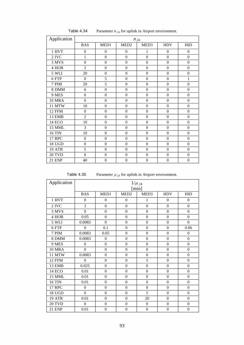
93
Table 4.34 Parameter n j\k for uplink in Airport environment.
Application n j\k
BAS MED1 MED2 MED3 HDV HID
1 HVT 0 0 0 1 0 0
2 IVC 1 0 0 0 0 0
3 MVS 0 0 0 0 0 0
4 HOB 2 0 0 0 0 0
5 WLI 20 0 0 0 0 0
6 FTP 0 5 0 0 0 1
7 PIM 20 5 0 0 0 0
8 DMM 6 0 0 0 0 0
9 MES 0 0 0 0 0 0
10 MRA 0 0 0 0 0 0
11 MTW 10 0 0 0 0 0
12 FFM 0 0 0 0 0 0
13 EMB 2 0 0 0 0 0
14 ECO 10 0 0 0 0 0
15 MML 3 0 0 0 0 0
16 TIN 10 0 0 0 0 0
17 RPC 0 0 0 0 0 0
18 UGD 0 0 0 0 0 0
19 ATR 5 0 0 0 0 0
20 TVD 0 0 0 0 0 0
21 ENP 40 0 0 0 0 0
Table 4.35 Parameter j\k for uplink in Airport environment.
Application 1/ j\k
[min] BAS MED1 MED2 MED3 HDV HID
1 HVT 0 0 0 1 0 0
2 IVC 3 0 0 0 0 0
3 MVS 0 0 0 0 0 0
4 HOB 0.05 0 0 0 0 0
5 WLI 0.0083 0 0 0 0 0
6 FTP 0 0.1 0 0 0 0.06
7 PIM 0.0083 0.05 0 0 0 0
8 DMM 0.0083 0 0 0 0 0
9 MES 0 0 0 0 0 0
10 MRA 0 0 0 0 0 0
11 MTW 0.0083 0 0 0 0 0
12 FFM 0 0 0 5 0 0
13 EMB 0.025 0 0 0 0 0
14 ECO 0.01 0 0 0 0 0
15 MML 0.01 0 0 0 0 0
16 TIN 0.01 0 0 0 0 0
17 RPC 0 0 0 0 0 0
18 UGD 0 0 0 5 0 0
19 ATR 0.01 0 0 20 0 0
20 TVD 0 0 0 0 0 0
21 ENP 0.01 0 0 0 0 0
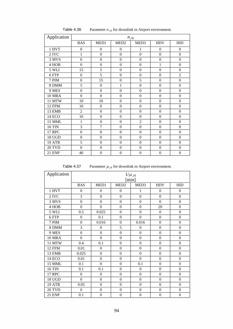
94
Table 4.36 Parameter n j\k for downlink in Airport environment.
Application n j\k
BAS MED1 MED2 MED3 HDV HID
1 HVT 0 0 0 1 0 0
2 IVC 1 0 0 0 0 0
3 MVS 0 0 0 0 0 0
4 HOB 0 0 0 0 1 0
5 WLI 15 5 0 0 0 0
6 FTP 0 5 0 0 0 2
7 PIM 0 15 0 5 0 0
8 DMM 5 0 1 0 0 0
9 MES 0 0 0 0 0 0
10 MRA 0 0 0 0 0 0
11 MTW 10 10 0 0 0 0
12 FFM 10 0 0 0 0 0
13 EMB 2 0 0 0 0 0
14 ECO 10 0 0 0 0 0
15 MML 1 0 0 2 0 0
16 TIN 3 7 0 0 0 0
17 RPC 0 0 0 0 0 0
18 UGD 0 0 0 0 0 0
19 ATR 5 0 0 0 0 0
20 TVD 0 0 0 0 0 0
21 ENP 40 0 0 0 0 0
Table 4.37 Parameter j\k for downlink in Airport environment.
Application 1/ j\k
[min] BAS MED1 MED2 MED3 HDV HID
1 HVT 0 0 0 1 0 0
2 IVC 3 0 0 0 0 0
3 MVS 0 0 0 0 0 0
4 HOB 0 0 0 0 20 0
5 WLI 0.5 0.025 0 0 0 0
6 FTP 0 0.1 0 0 0 0
7 PIM 0 0.016 0 0.016 0 0
8 DMM 3 0 5 0 0 0
9 MES 0 0 0 0 0 0
10 MRA 0 0 0 0 0 0
11 MTW 0.4 0.1 0 0 0 0
12 FFM 0.01 0 0 0 0 0
13 EMB 0.025 0 0 0 0 0
14 ECO 0.01 0 0 0 0 0
15 MML 0.1 0 0 0.1 0 0
16 TIN 0.1 0.1 0 0 0 0
17 RPC 0 0 0 0 0 0
18 UGD 0 0 0 0 0 0
19 ATR 0.05 0 0 0 0 0
20 TVD 0 0 0 0 0 0
21 ENP 0.1 0 0 0 0 0
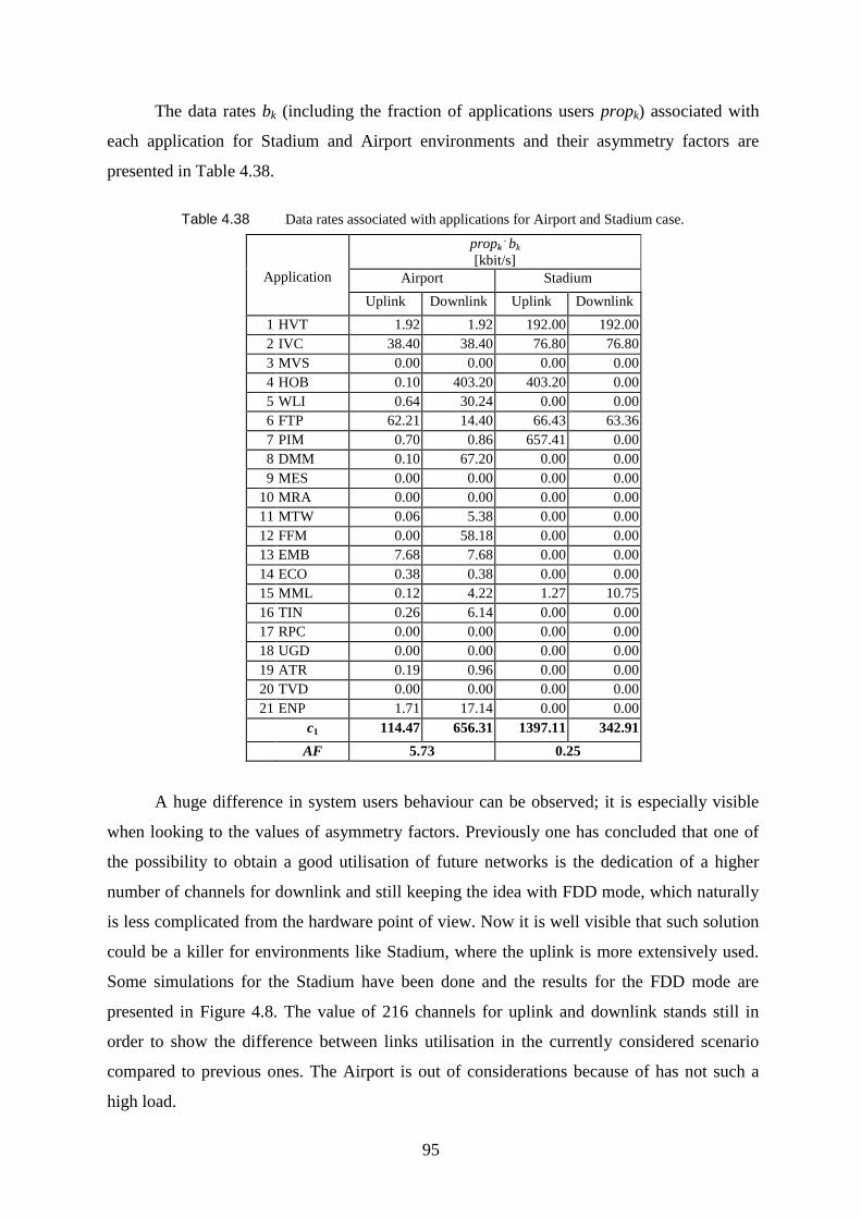
95
The data rates bk (including the fraction of applications users propk) associated with
each application for Stadium and Airport environments and their asymmetry factors are
presented in Table 4.38.
Table 4.38 Data rates associated with applications for Airport and Stadium case.
Application
propk . bk
[kbit/s]
Airport Stadium
Uplink Downlink Uplink Downlink
1 HVT 1.92 1.92 192.00 192.00
2 IVC 38.40 38.40 76.80 76.80
3 MVS 0.00 0.00 0.00 0.00
4 HOB 0.10 403.20 403.20 0.00
5 WLI 0.64 30.24 0.00 0.00
6 FTP 62.21 14.40 66.43 63.36
7 PIM 0.70 0.86 657.41 0.00
8 DMM 0.10 67.20 0.00 0.00
9 MES 0.00 0.00 0.00 0.00
10 MRA 0.00 0.00 0.00 0.00
11 MTW 0.06 5.38 0.00 0.00
12 FFM 0.00 58.18 0.00 0.00
13 EMB 7.68 7.68 0.00 0.00
14 ECO 0.38 0.38 0.00 0.00
15 MML 0.12 4.22 1.27 10.75
16 TIN 0.26 6.14 0.00 0.00
17 RPC 0.00 0.00 0.00 0.00
18 UGD 0.00 0.00 0.00 0.00
19 ATR 0.19 0.96 0.00 0.00
20 TVD 0.00 0.00 0.00 0.00
21 ENP 1.71 17.14 0.00 0.00
c1 114.47 656.31 1397.11 342.91
AF 5.73 0.25
A huge difference in system users behaviour can be observed; it is especially visible
when looking to the values of asymmetry factors. Previously one has concluded that one of
the possibility to obtain a good utilisation of future networks is the dedication of a higher
number of channels for downlink and still keeping the idea with FDD mode, which naturally
is less complicated from the hardware point of view. Now it is well visible that such solution
could be a killer for environments like Stadium, where the uplink is more extensively used.
Some simulations for the Stadium have been done and the results for the FDD mode are
presented in Figure 4.8. The value of 216 channels for uplink and downlink stands still in
order to show the difference between links utilisation in the currently considered scenario
compared to previous ones. The Airport is out of considerations because of has not such a
high load.
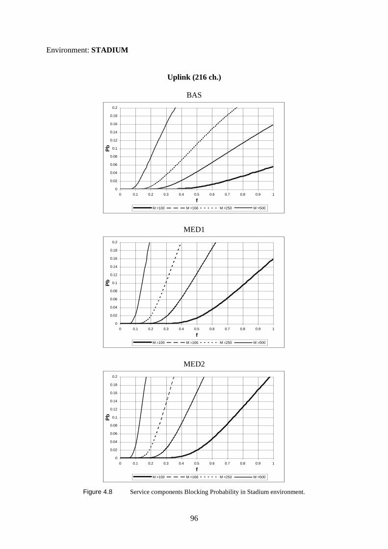
96
Environment: STADIUM
Uplink (216 ch.)
BAS
0
0.02
0.04
0.06
0.08
0.1
0.12
0.14
0.16
0.18
0.2
0 0.1 0.2 0.3 0.4 0.5 0.6 0.7 0.8 0.9 1
f
Pb
M =100 M =166 M =250 M =500
MED1
0
0.02
0.04
0.06
0.08
0.1
0.12
0.14
0.16
0.18
0.2
0 0.1 0.2 0.3 0.4 0.5 0.6 0.7 0.8 0.9 1
f
Pb
M =100 M =166 M =250 M =500
MED2
0
0.02
0.04
0.06
0.08
0.1
0.12
0.14
0.16
0.18
0.2
0 0.1 0.2 0.3 0.4 0.5 0.6 0.7 0.8 0.9 1
f
Pb
M =100 M =166 M =250 M =500
Figure 4.8 Service components Blocking Probability in Stadium environment.
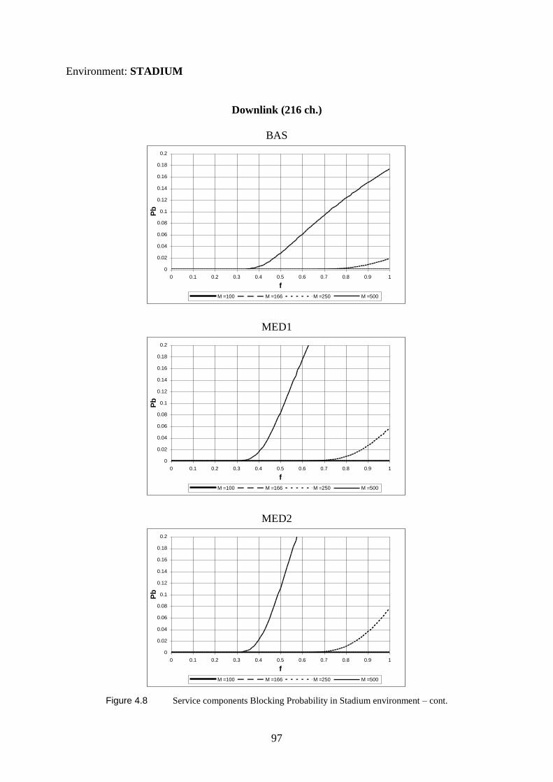
97
Environment: STADIUM
Downlink (216 ch.)
BAS
0
0.02
0.04
0.06
0.08
0.1
0.12
0.14
0.16
0.18
0.2
0 0.1 0.2 0.3 0.4 0.5 0.6 0.7 0.8 0.9 1
f
Pb
M =100 M =166 M =250 M =500
MED1
0
0.02
0.04
0.06
0.08
0.1
0.12
0.14
0.16
0.18
0.2
0 0.1 0.2 0.3 0.4 0.5 0.6 0.7 0.8 0.9 1
f
Pb
M =100 M =166 M =250 M =500
MED2
0
0.02
0.04
0.06
0.08
0.1
0.12
0.14
0.16
0.18
0.2
0 0.1 0.2 0.3 0.4 0.5 0.6 0.7 0.8 0.9 1
f
Pb
M =100 M =166 M =250 M =500
Figure 4.8 Service components Blocking Probability in Stadium environment – cont.
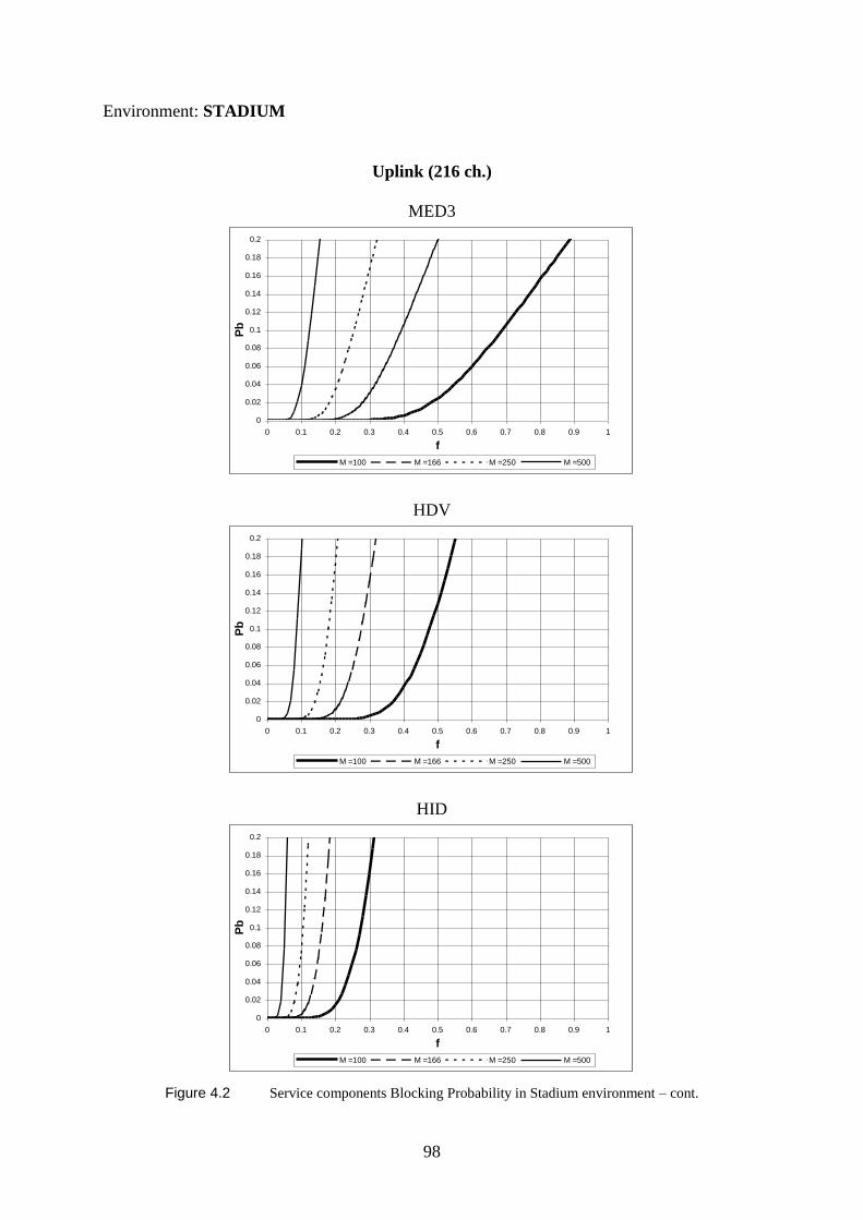
98
Environment: STADIUM
Uplink (216 ch.)
MED3
0
0.02
0.04
0.06
0.08
0.1
0.12
0.14
0.16
0.18
0.2
0 0.1 0.2 0.3 0.4 0.5 0.6 0.7 0.8 0.9 1
f
Pb
M =100 M =166 M =250 M =500
HDV
0
0.02
0.04
0.06
0.08
0.1
0.12
0.14
0.16
0.18
0.2
0 0.1 0.2 0.3 0.4 0.5 0.6 0.7 0.8 0.9 1
f
Pb
M =100 M =166 M =250 M =500
HID
0
0.02
0.04
0.06
0.08
0.1
0.12
0.14
0.16
0.18
0.2
0 0.1 0.2 0.3 0.4 0.5 0.6 0.7 0.8 0.9 1
f
Pb
M =100 M =166 M =250 M =500
Figure 4.2 Service components Blocking Probability in Stadium environment – cont.
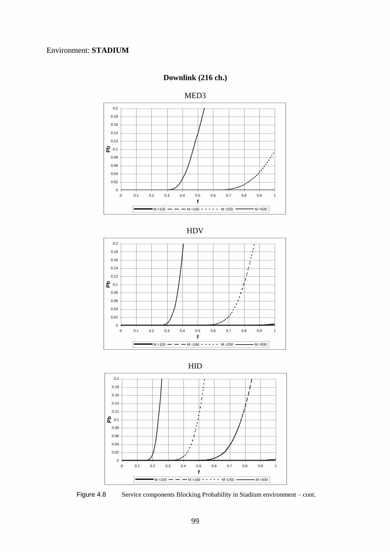
99
Environment: STADIUM
Downlink (216 ch.)
MED3
0
0.02
0.04
0.06
0.08
0.1
0.12
0.14
0.16
0.18
0.2
0 0.1 0.2 0.3 0.4 0.5 0.6 0.7 0.8 0.9 1
f
Pb
M =100 M =166 M =250 M =500
HDV
0
0.02
0.04
0.06
0.08
0.1
0.12
0.14
0.16
0.18
0.2
0 0.1 0.2 0.3 0.4 0.5 0.6 0.7 0.8 0.9 1
f
Pb
M =100 M =166 M =250 M =500
HID
0
0.02
0.04
0.06
0.08
0.1
0.12
0.14
0.16
0.18
0.2
0 0.1 0.2 0.3 0.4 0.5 0.6 0.7 0.8 0.9 1
f
Pb
M =100 M =166 M =250 M =500
Figure 4.8 Service components Blocking Probability in Stadium environment – cont.
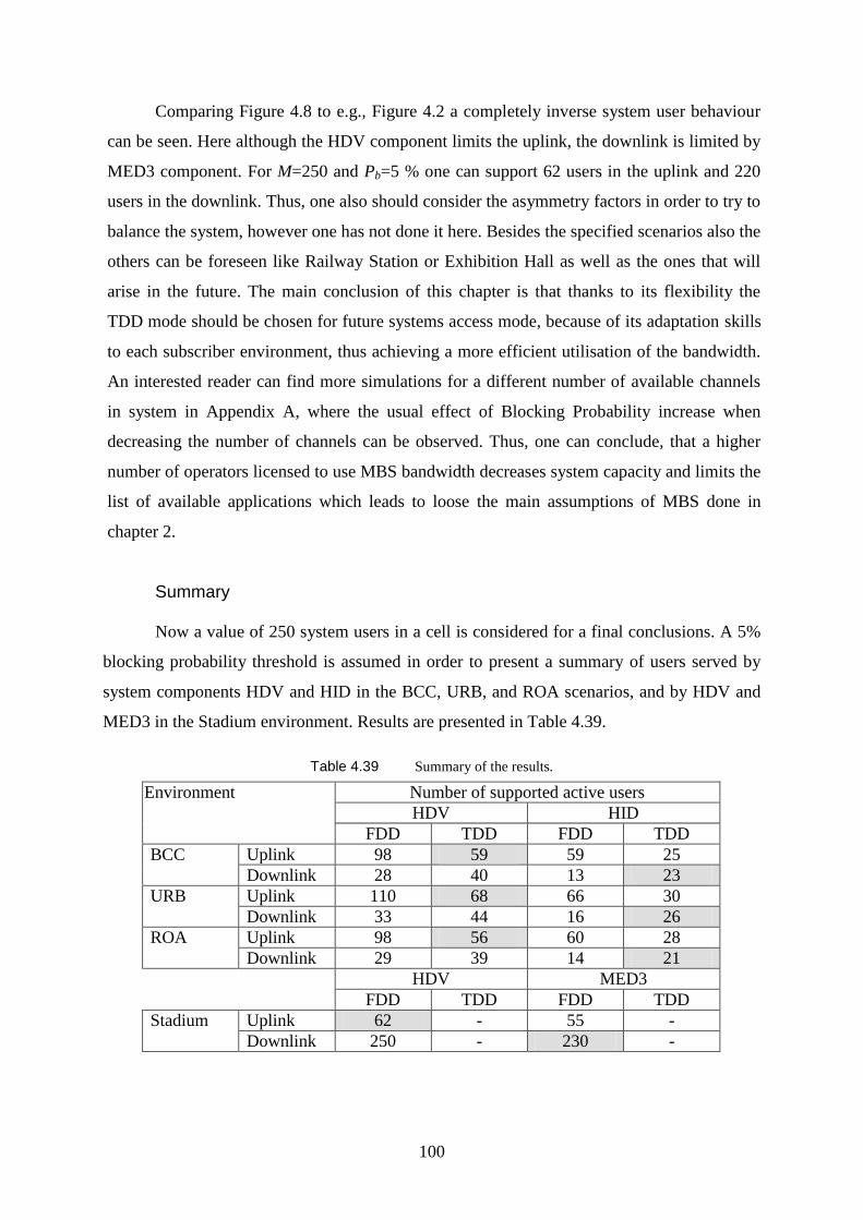
100
Comparing Figure 4.8 to e.g., Figure 4.2 a completely inverse system user behaviour
can be seen. Here although the HDV component limits the uplink, the downlink is limited by
MED3 component. For M=250 and Pb=5 % one can support 62 users in the uplink and 220
users in the downlink. Thus, one also should consider the asymmetry factors in order to try to
balance the system, however one has not done it here. Besides the specified scenarios also the
others can be foreseen like Railway Station or Exhibition Hall as well as the ones that will
arise in the future. The main conclusion of this chapter is that thanks to its flexibility the
TDD mode should be chosen for future systems access mode, because of its adaptation skills
to each subscriber environment, thus achieving a more efficient utilisation of the bandwidth.
An interested reader can find more simulations for a different number of available channels
in system in Appendix A, where the usual effect of Blocking Probability increase when
decreasing the number of channels can be observed. Thus, one can conclude, that a higher
number of operators licensed to use MBS bandwidth decreases system capacity and limits the
list of available applications which leads to loose the main assumptions of MBS done in
chapter 2.
Summary
Now a value of 250 system users in a cell is considered for a final conclusions. A 5%
blocking probability threshold is assumed in order to present a summary of users served by
system components HDV and HID in the BCC, URB, and ROA scenarios, and by HDV and
MED3 in the Stadium environment. Results are presented in Table 4.39.
Table 4.39 Summary of the results.
Environment Number of supported active users
HDV HID
FDD TDD FDD TDD
BCC Uplink 98 59 59 25
Downlink 28 40 13 23
URB Uplink 110 68 66 30
Downlink 33 44 16 26
ROA Uplink 98 56 60 28
Downlink 29 39 14 21
HDV MED3
FDD TDD FDD TDD
Stadium Uplink 62 - 55 -
Downlink 250 - 230 -
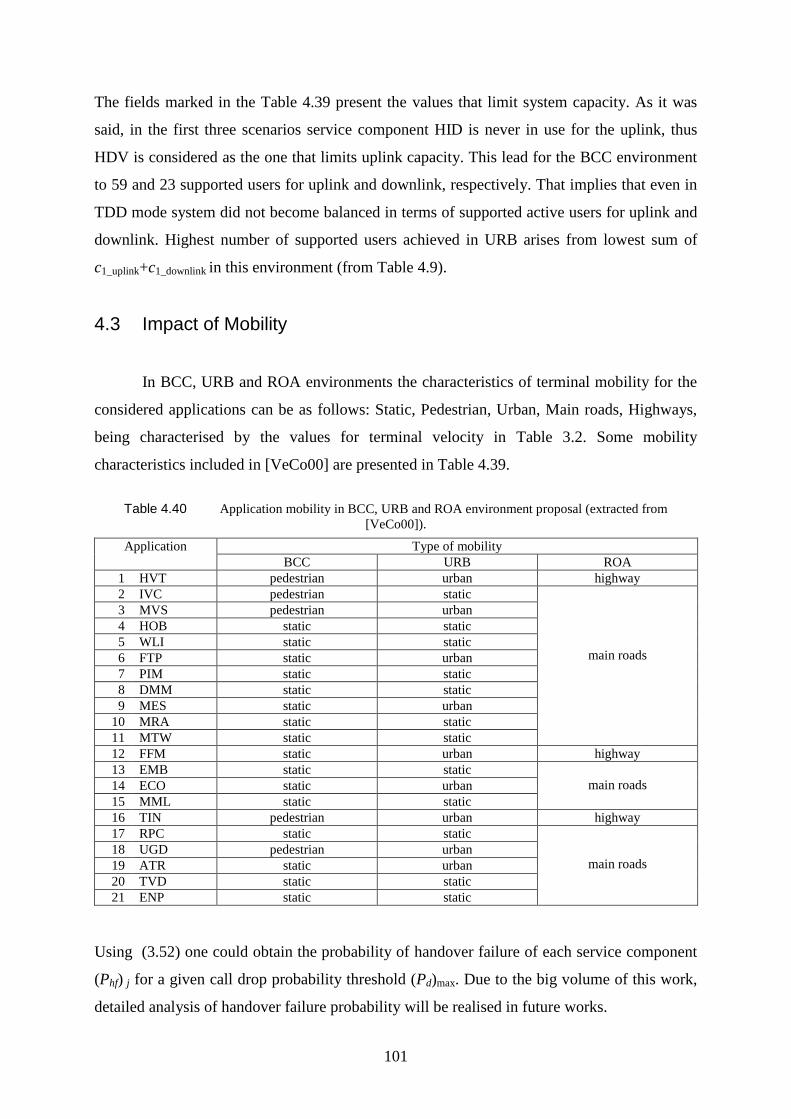
101
The fields marked in the Table 4.39 present the values that limit system capacity. As it was
said, in the first three scenarios service component HID is never in use for the uplink, thus
HDV is considered as the one that limits uplink capacity. This lead for the BCC environment
to 59 and 23 supported users for uplink and downlink, respectively. That implies that even in
TDD mode system did not become balanced in terms of supported active users for uplink and
downlink. Highest number of supported users achieved in URB arises from lowest sum of
c1_uplink+c1_downlink in this environment (from Table 4.9).
4.3 Impact of Mobility
In BCC, URB and ROA environments the characteristics of terminal mobility for the
considered applications can be as follows: Static, Pedestrian, Urban, Main roads, Highways,
being characterised by the values for terminal velocity in Table 3.2. Some mobility
characteristics included in [VeCo00] are presented in Table 4.39.
Table 4.40 Application mobility in BCC, URB and ROA environment proposal (extracted from
[VeCo00]).
Application Type of mobility
BCC URB ROA
1 HVT pedestrian urban highway
2 IVC pedestrian static
main roads
3 MVS pedestrian urban
4 HOB static static
5 WLI static static
6 FTP static urban
7 PIM static static
8 DMM static static
9 MES static urban
10 MRA static static
11 MTW static static
12 FFM static urban highway
13 EMB static static
main roads 14 ECO static urban
15 MML static static
16 TIN pedestrian urban highway
17 RPC static static
main roads 18 UGD pedestrian urban
19 ATR static urban
20 TVD static static
21 ENP static static
Using (3.52) one could obtain the probability of handover failure of each service component
(Phf) j for a given call drop probability threshold (Pd)max. Due to the big volume of this work,
detailed analysis of handover failure probability will be realised in future works.

102
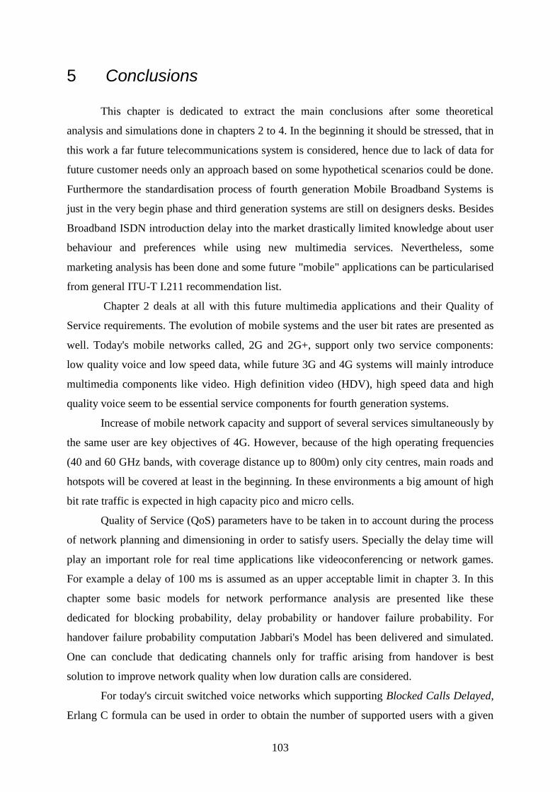
103
5 Conclusions
This chapter is dedicated to extract the main conclusions after some theoretical
analysis and simulations done in chapters 2 to 4. In the beginning it should be stressed, that in
this work a far future telecommunications system is considered, hence due to lack of data for
future customer needs only an approach based on some hypothetical scenarios could be done.
Furthermore the standardisation process of fourth generation Mobile Broadband Systems is
just in the very begin phase and third generation systems are still on designers desks. Besides
Broadband ISDN introduction delay into the market drastically limited knowledge about user
behaviour and preferences while using new multimedia services. Nevertheless, some
marketing analysis has been done and some future "mobile" applications can be particularised
from general ITU-T I.211 recommendation list.
Chapter 2 deals at all with this future multimedia applications and their Quality of
Service requirements. The evolution of mobile systems and the user bit rates are presented as
well. Today's mobile networks called, 2G and 2G+, support only two service components:
low quality voice and low speed data, while future 3G and 4G systems will mainly introduce
multimedia components like video. High definition video (HDV), high speed data and high
quality voice seem to be essential service components for fourth generation systems.
Increase of mobile network capacity and support of several services simultaneously by
the same user are key objectives of 4G. However, because of the high operating frequencies
(40 and 60 GHz bands, with coverage distance up to 800m) only city centres, main roads and
hotspots will be covered at least in the beginning. In these environments a big amount of high
bit rate traffic is expected in high capacity pico and micro cells.
Quality of Service (QoS) parameters have to be taken in to account during the process
of network planning and dimensioning in order to satisfy users. Specially the delay time will
play an important role for real time applications like videoconferencing or network games.
For example a delay of 100 ms is assumed as an upper acceptable limit in chapter 3. In this
chapter some basic models for network performance analysis are presented like these
dedicated for blocking probability, delay probability or handover failure probability. For
handover failure probability computation Jabbari's Model has been delivered and simulated.
One can conclude that dedicating channels only for traffic arising from handover is best
solution to improve network quality when low duration calls are considered.
For today's circuit switched voice networks which supporting Blocked Calls Delayed,
Erlang C formula can be used in order to obtain the number of supported users with a given
104
allowable delay. In blocking probability computations one usually is interested in number of
supported users. Erlang B is the most popular traffic engineers tool for voice networks traffic
dimensioning today, but its usage is limited only for voice networks. The modelling of future
Multiservice networks is delivered in chapter 3.
Markov Modulated Poisson Processes (MMPP) are used to compute blocking
probability, with different arrival rates for different service components. Because the number
of channels available in MBS cells seems to be similar to the expected number of users in a
cell, we cannot assume that new call arrival is independent of the number of calls being in
progress. Thus, Bernoulli case of BPP theory has been chosen in order to simulate MMPP
process. Furthermore, independence in service components activation during application
service time is assumed, allowing the model to capture traffic burstiness which is very
important for a correct simulation of future networks, with their data applications (e-mail,
WEB browsing) bursty nature.
In chapter 4 some foreseen scenarios are simulated using BPP theory. More than 20
applications getting access to 6 service components with data rates from 384 kbit/s up to
31872 kbit/s were considered. The set of simulations of blocking probability as a function of
active users gives an overall view of forecasted future environments. Three of the main
environments for future MBS are: Business City Centre, Urban, Main Roads. As it was
remarked, in these scenarios service component HID is never in use for the uplink, thus HDV
is considered as the one that limits uplink capacity. This leads for example in the BCC
environment, to 59 and 23 supported users for uplink and downlink, respectively. That
implies that even in TDD mode the system did not become balanced in terms of supported
active users for uplink and downlink. The highest number of supported users achieved in
URB arises from lowest sum of c1_uplink+c1_downlink in this environment.
Furthermore one also presents an analysis of hotspots, where users behaviour can be
extremely different. Such situations have to be also taken into account in system
standardisation.
Comparing results and charts from chapter 4 to these presented in Appendix A one can
observe an effect of increase of blocking probability while decreasing number of available in
cell channels. Decrease of number of available in system channels leads also to some
limitations in served applications list e.g., in FDD mode only few scenarios (mainly for 2
operators) are capable to support Fast Ethernet connections.
105
Future Works
Besides trying to achieve a balanced system by changing the number of channels in
uplink and downlink, future work will be mainly focused in market and real statistics (e.g.
from B-ISDN or UMTS networks) analysis in order to improve input parameters and obtain
real results. Some other environments can be simulated, like exhibition hall or port (fleet
management together with subscribers services) to make system capacity dimensioning more
effective. Furthermore to control overall network planning process, propagation models (for
40 GHz and 60 GHz) should be attached to this work as well. Influence of the impact of
terminal mobility on traffic performance also will take part of future works. Some analysis
concerning to delay time in radio interface (Medium Access Control protocol study) should
be done also.
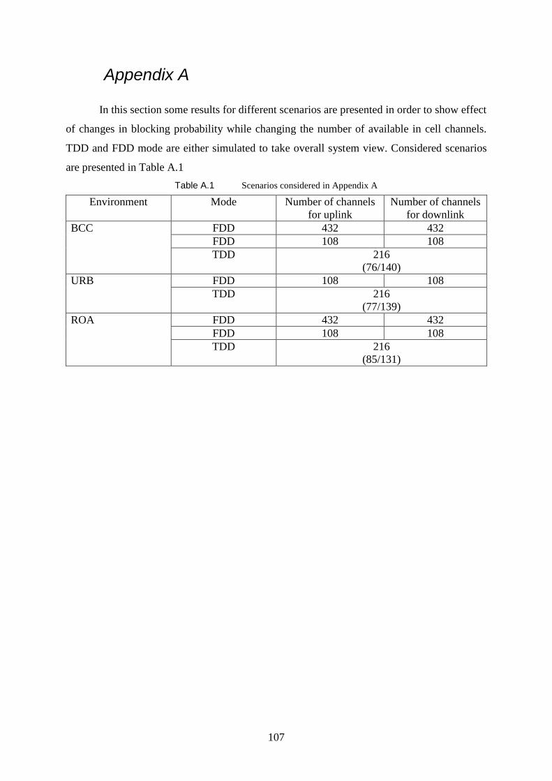
107
Appendix A In this section some results for different scenarios are presented in order to show effect
of changes in blocking probability while changing the number of available in cell channels.
TDD and FDD mode are either simulated to take overall system view. Considered scenarios
are presented in Table A.1
Table A.1 Scenarios considered in Appendix A
Environment Mode Number of channels
for uplink
Number of channels
for downlink
BCC FDD 432 432
FDD 108 108
TDD 216
(76/140)
URB FDD 108 108
TDD 216
(77/139)
ROA FDD 432 432
FDD 108 108
TDD 216
(85/131)
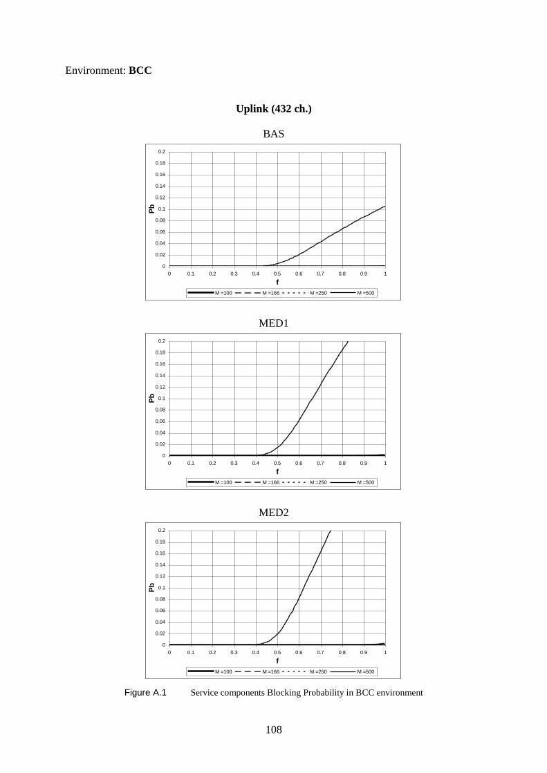
108
Environment: BCC
Uplink (432 ch.)
BAS
0
0.02
0.04
0.06
0.08
0.1
0.12
0.14
0.16
0.18
0.2
0 0.1 0.2 0.3 0.4 0.5 0.6 0.7 0.8 0.9 1
f
Pb
M =100 M =166 M =250 M =500
MED1
0
0.02
0.04
0.06
0.08
0.1
0.12
0.14
0.16
0.18
0.2
0 0.1 0.2 0.3 0.4 0.5 0.6 0.7 0.8 0.9 1
f
Pb
M =100 M =166 M =250 M =500
MED2
0
0.02
0.04
0.06
0.08
0.1
0.12
0.14
0.16
0.18
0.2
0 0.1 0.2 0.3 0.4 0.5 0.6 0.7 0.8 0.9 1
f
Pb
M =100 M =166 M =250 M =500
Figure A.1 Service components Blocking Probability in BCC environment

109
Environment: BCC
Downlink (432 ch.)
BAS
0
0.02
0.04
0.06
0.08
0.1
0.12
0.14
0.16
0.18
0.2
0 0.1 0.2 0.3 0.4 0.5 0.6 0.7 0.8 0.9 1
f
Pb
M =100 M =166 M =250 M =500
MED1
0
0.02
0.04
0.06
0.08
0.1
0.12
0.14
0.16
0.18
0.2
0 0.1 0.2 0.3 0.4 0.5 0.6 0.7 0.8 0.9 1
f
Pb
M =100 M =166 M =250 M =500
MED2
0
0.02
0.04
0.06
0.08
0.1
0.12
0.14
0.16
0.18
0.2
0 0.1 0.2 0.3 0.4 0.5 0.6 0.7 0.8 0.9 1
f
Pb
M =100 M =166 M =250 M =500
Figure A.1 Service components Blocking Probability in BCC environment – cont.
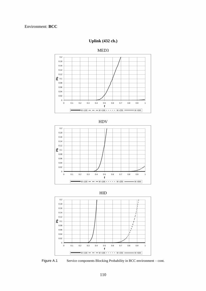
110
Environment: BCC
Uplink (432 ch.)
MED3
0
0.02
0.04
0.06
0.08
0.1
0.12
0.14
0.16
0.18
0.2
0 0.1 0.2 0.3 0.4 0.5 0.6 0.7 0.8 0.9 1
f
Pb
M =100 M =166 M =250 M =500
HDV
0
0.02
0.04
0.06
0.08
0.1
0.12
0.14
0.16
0.18
0.2
0 0.1 0.2 0.3 0.4 0.5 0.6 0.7 0.8 0.9 1
f
Pb
M =100 M =166 M =250 M =500
HID
0
0.02
0.04
0.06
0.08
0.1
0.12
0.14
0.16
0.18
0.2
0 0.1 0.2 0.3 0.4 0.5 0.6 0.7 0.8 0.9 1
f
Pb
M =100 M =166 M =250 M =500
Figure A.1 Service components Blocking Probability in BCC environment – cont.
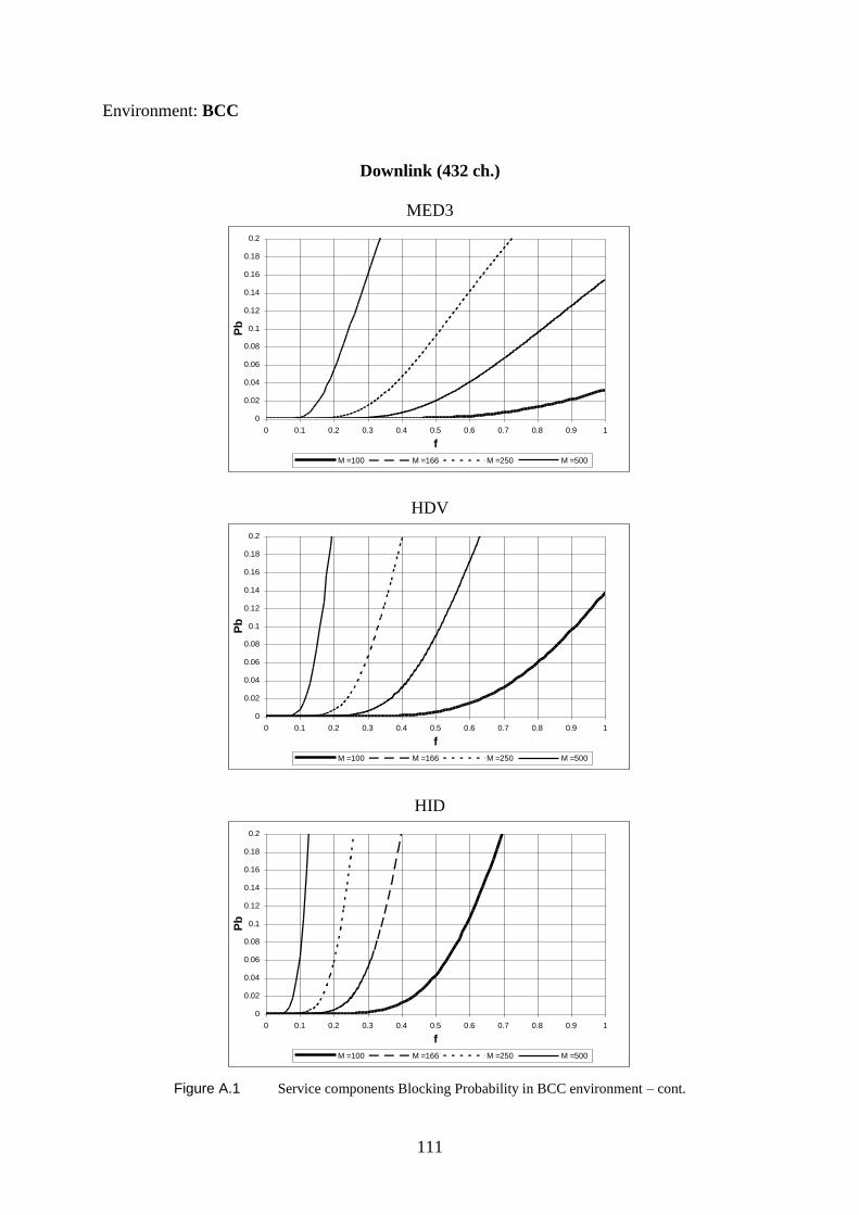
111
Environment: BCC
Downlink (432 ch.)
MED3
0
0.02
0.04
0.06
0.08
0.1
0.12
0.14
0.16
0.18
0.2
0 0.1 0.2 0.3 0.4 0.5 0.6 0.7 0.8 0.9 1
f
Pb
M =100 M =166 M =250 M =500
HDV
0
0.02
0.04
0.06
0.08
0.1
0.12
0.14
0.16
0.18
0.2
0 0.1 0.2 0.3 0.4 0.5 0.6 0.7 0.8 0.9 1
f
Pb
M =100 M =166 M =250 M =500
HID
0
0.02
0.04
0.06
0.08
0.1
0.12
0.14
0.16
0.18
0.2
0 0.1 0.2 0.3 0.4 0.5 0.6 0.7 0.8 0.9 1
f
Pb
M =100 M =166 M =250 M =500
Figure A.1 Service components Blocking Probability in BCC environment – cont.
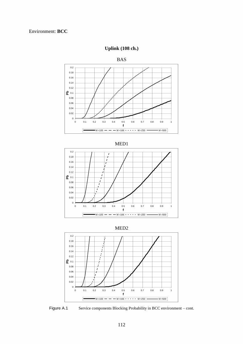
112
Environment: BCC
Uplink (108 ch.)
BAS
0
0.02
0.04
0.06
0.08
0.1
0.12
0.14
0.16
0.18
0.2
0 0.1 0.2 0.3 0.4 0.5 0.6 0.7 0.8 0.9 1
f
Pb
M =100 M =166 M =250 M =500
MED1
0
0.02
0.04
0.06
0.08
0.1
0.12
0.14
0.16
0.18
0.2
0 0.1 0.2 0.3 0.4 0.5 0.6 0.7 0.8 0.9 1
f
Pb
M =100 M =166 M =250 M =500
MED2
0
0.02
0.04
0.06
0.08
0.1
0.12
0.14
0.16
0.18
0.2
0 0.1 0.2 0.3 0.4 0.5 0.6 0.7 0.8 0.9 1
f
Pb
M =100 M =166 M =250 M =500
Figure A.1 Service components Blocking Probability in BCC environment – cont.

113
Environment: BCC
Downlink (108 ch.)
BAS
0
0.02
0.04
0.06
0.08
0.1
0.12
0.14
0.16
0.18
0.2
0 0.1 0.2 0.3 0.4 0.5 0.6 0.7 0.8 0.9 1
f
Pb
M =100 M =166 M =250 M =500
MED1
0
0.02
0.04
0.06
0.08
0.1
0.12
0.14
0.16
0.18
0.2
0 0.1 0.2 0.3 0.4 0.5 0.6 0.7 0.8 0.9 1
f
Pb
M =100 M =166 M =250 M =500
MED2
0
0.02
0.04
0.06
0.08
0.1
0.12
0.14
0.16
0.18
0.2
0 0.1 0.2 0.3 0.4 0.5 0.6 0.7 0.8 0.9 1
f
Pb
M =100 M =166 M =250 M =500
Figure A.1 Service components Blocking Probability in BCC environment – cont.
114
Environment: BCC
Uplink (108 ch.)
MED3
0
0.02
0.04
0.06
0.08
0.1
0.12
0.14
0.16
0.18
0.2
0 0.1 0.2 0.3 0.4 0.5 0.6 0.7 0.8 0.9 1
f
Pb
M =100 M =166 M =250 M =500
HDV
0
0.02
0.04
0.06
0.08
0.1
0.12
0.14
0.16
0.18
0.2
0 0.1 0.2 0.3 0.4 0.5 0.6 0.7 0.8 0.9 1
f
Pb
M =100 M =166 M =250 M =500
HID
0
0.02
0.04
0.06
0.08
0.1
0.12
0.14
0.16
0.18
0.2
0 0.1 0.2 0.3 0.4 0.5 0.6 0.7 0.8 0.9 1
f
Pb
M =100 M =166 M =250 M =500
Figure A.1 Service components Blocking Probability in BCC environment – cont.
115
Environment: BCC
Downlink (108 ch.)
MED3
0
0.02
0.04
0.06
0.08
0.1
0.12
0.14
0.16
0.18
0.2
0 0.1 0.2 0.3 0.4 0.5 0.6 0.7 0.8 0.9 1
f
Pb
M =100 M =166 M =250 M =500
HDV
0
0.02
0.04
0.06
0.08
0.1
0.12
0.14
0.16
0.18
0.2
0 0.1 0.2 0.3 0.4 0.5 0.6 0.7 0.8 0.9 1
f
Pb
M =100 M =166 M =250 M =500
HID
0
0.02
0.04
0.06
0.08
0.1
0.12
0.14
0.16
0.18
0.2
0 0.1 0.2 0.3 0.4 0.5 0.6 0.7 0.8 0.9 1
f
Pb
M =100 M =166 M =250 M =500
Figure A.1 Service components Blocking Probability in BCC environment – cont.

116
Environment: BCC
Uplink (76 ch.)
BAS
0
0.02
0.04
0.06
0.08
0.1
0.12
0.14
0.16
0.18
0.2
0 0.1 0.2 0.3 0.4 0.5 0.6 0.7 0.8 0.9 1
f
Pb
M =100 M =166 M =250 M =500
MED1
0
0.02
0.04
0.06
0.08
0.1
0.12
0.14
0.16
0.18
0.2
0 0.1 0.2 0.3 0.4 0.5 0.6 0.7 0.8 0.9 1
f
Pb
M =100 M =166 M =250 M =500
MED2
0
0.02
0.04
0.06
0.08
0.1
0.12
0.14
0.16
0.18
0.2
0 0.1 0.2 0.3 0.4 0.5 0.6 0.7 0.8 0.9 1
f
Pb
M =100 M =166 M =250 M =500
Figure A.1 Service components Blocking Probability in BCC environment – cont.

117
Environment: BCC
Downlink (140 ch.)
BAS
0
0.02
0.04
0.06
0.08
0.1
0.12
0.14
0.16
0.18
0.2
0 0.1 0.2 0.3 0.4 0.5 0.6 0.7 0.8 0.9 1
f
Pb
M =100 M =166 M =250 M =500
MED1
0
0.02
0.04
0.06
0.08
0.1
0.12
0.14
0.16
0.18
0.2
0 0.1 0.2 0.3 0.4 0.5 0.6 0.7 0.8 0.9 1
f
Pb
M =100 M =166 M =250 M =500
MED2
0
0.02
0.04
0.06
0.08
0.1
0.12
0.14
0.16
0.18
0.2
0 0.1 0.2 0.3 0.4 0.5 0.6 0.7 0.8 0.9 1
f
Pb
M =100 M =166 M =250 M =500
Figure A.1 Service components Blocking Probability in BCC environment – cont.
118
Environment: BCC
Uplink (76 ch.)
MED3
0
0.02
0.04
0.06
0.08
0.1
0.12
0.14
0.16
0.18
0.2
0 0.1 0.2 0.3 0.4 0.5 0.6 0.7 0.8 0.9 1
f
Pb
M =100 M =166 M =250 M =500
HDV
0
0.02
0.04
0.06
0.08
0.1
0.12
0.14
0.16
0.18
0.2
0 0.1 0.2 0.3 0.4 0.5 0.6 0.7 0.8 0.9 1
f
Pb
M =100 M =166 M =250 M =500
HID
0
0.02
0.04
0.06
0.08
0.1
0.12
0.14
0.16
0.18
0.2
0 0.1 0.2 0.3 0.4 0.5 0.6 0.7 0.8 0.9 1
f
Pb
M =100 M =166 M =250 M =500
Figure A.1 Service components Blocking Probability in BCC environment – cont.

119
Environment: BCC
Downlink (140 ch.)
MED3
0
0.02
0.04
0.06
0.08
0.1
0.12
0.14
0.16
0.18
0.2
0 0.1 0.2 0.3 0.4 0.5 0.6 0.7 0.8 0.9 1
f
Pb
M =100 M =166 M =250 M =500
HDV
0
0.02
0.04
0.06
0.08
0.1
0.12
0.14
0.16
0.18
0.2
0 0.1 0.2 0.3 0.4 0.5 0.6 0.7 0.8 0.9 1
f
Pb
M =100 M =166 M =250 M =500
HID
0
0.02
0.04
0.06
0.08
0.1
0.12
0.14
0.16
0.18
0.2
0 0.1 0.2 0.3 0.4 0.5 0.6 0.7 0.8 0.9 1
f
Pb
M =100 M =166 M =250 M =500
Figure A.1 Service components Blocking Probability in BCC environment – cont.
120
Environment: URB
Uplink (108 ch.)
BAS
0
0.02
0.04
0.06
0.08
0.1
0.12
0.14
0.16
0.18
0.2
0 0.1 0.2 0.3 0.4 0.5 0.6 0.7 0.8 0.9 1
f
Pb
M =100 M =166 M =250 M =500
MED1
0
0.02
0.04
0.06
0.08
0.1
0.12
0.14
0.16
0.18
0.2
0 0.1 0.2 0.3 0.4 0.5 0.6 0.7 0.8 0.9 1
f
Pb
M =100 M =166 M =250 M =500
MED2
0
0.02
0.04
0.06
0.08
0.1
0.12
0.14
0.16
0.18
0.2
0 0.1 0.2 0.3 0.4 0.5 0.6 0.7 0.8 0.9 1
f
Pb
M =100 M =166 M =250 M =500
Figure A.2 Service components Blocking Probability in URB environment.
121
Environment: URB
Downlink (108 ch.)
BAS
0
0.02
0.04
0.06
0.08
0.1
0.12
0.14
0.16
0.18
0.2
0 0.1 0.2 0.3 0.4 0.5 0.6 0.7 0.8 0.9 1
f
Pb
M =100 M =166 M =250 M =500
MED1
0
0.02
0.04
0.06
0.08
0.1
0.12
0.14
0.16
0.18
0.2
0 0.1 0.2 0.3 0.4 0.5 0.6 0.7 0.8 0.9 1
f
Pb
M =100 M =166 M =250 M =500
MED2
0
0.02
0.04
0.06
0.08
0.1
0.12
0.14
0.16
0.18
0.2
0 0.1 0.2 0.3 0.4 0.5 0.6 0.7 0.8 0.9 1
f
Pb
M =100 M =166 M =250 M =500
Figure A.2 Service components Blocking Probability in URB environment – cont.
122
Environment: URB
Uplink (108 ch.)
MED3
0
0.02
0.04
0.06
0.08
0.1
0.12
0.14
0.16
0.18
0.2
0 0.1 0.2 0.3 0.4 0.5 0.6 0.7 0.8 0.9 1
f
Pb
M =100 M =166 M =250 M =500
HDV
0
0.02
0.04
0.06
0.08
0.1
0.12
0.14
0.16
0.18
0.2
0 0.1 0.2 0.3 0.4 0.5 0.6 0.7 0.8 0.9 1
f
Pb
M =100 M =166 M =250 M =500
HID
0
0.02
0.04
0.06
0.08
0.1
0.12
0.14
0.16
0.18
0.2
0 0.1 0.2 0.3 0.4 0.5 0.6 0.7 0.8 0.9 1
f
Pb
M =100 M =166 M =250 M =500
Figure A.2 Service components Blocking Probability in URB environment – cont.
123
Environment: URB
Downlink (108 ch.)
MED3
0
0.02
0.04
0.06
0.08
0.1
0.12
0.14
0.16
0.18
0.2
0 0.1 0.2 0.3 0.4 0.5 0.6 0.7 0.8 0.9 1
f
Pb
M =100 M =166 M =250 M =500
HDV
0
0.02
0.04
0.06
0.08
0.1
0.12
0.14
0.16
0.18
0.2
0 0.1 0.2 0.3 0.4 0.5 0.6 0.7 0.8 0.9 1
f
Pb
M =100 M =166 M =250 M =500
HID
0
0.02
0.04
0.06
0.08
0.1
0.12
0.14
0.16
0.18
0.2
0 0.1 0.2 0.3 0.4 0.5 0.6 0.7 0.8 0.9 1
f
Pb
M =100 M =166 M =250 M =500
Figure A.2 Service components Blocking Probability in URB environment – cont.
124
Environment: URB
Uplink (77 ch.)
BAS
0
0.02
0.04
0.06
0.08
0.1
0.12
0.14
0.16
0.18
0.2
0 0.1 0.2 0.3 0.4 0.5 0.6 0.7 0.8 0.9 1
f
Pb
M =100 M =166 M =250 M =500
MED1
0
0.02
0.04
0.06
0.08
0.1
0.12
0.14
0.16
0.18
0.2
0 0.1 0.2 0.3 0.4 0.5 0.6 0.7 0.8 0.9 1
f
Pb
M =100 M =166 M =250 M =500
MED2
0
0.02
0.04
0.06
0.08
0.1
0.12
0.14
0.16
0.18
0.2
0 0.1 0.2 0.3 0.4 0.5 0.6 0.7 0.8 0.9 1
f
Pb
M =100 M =166 M =250 M =500
Figure A.2 Service components Blocking Probability in URB environment – cont.
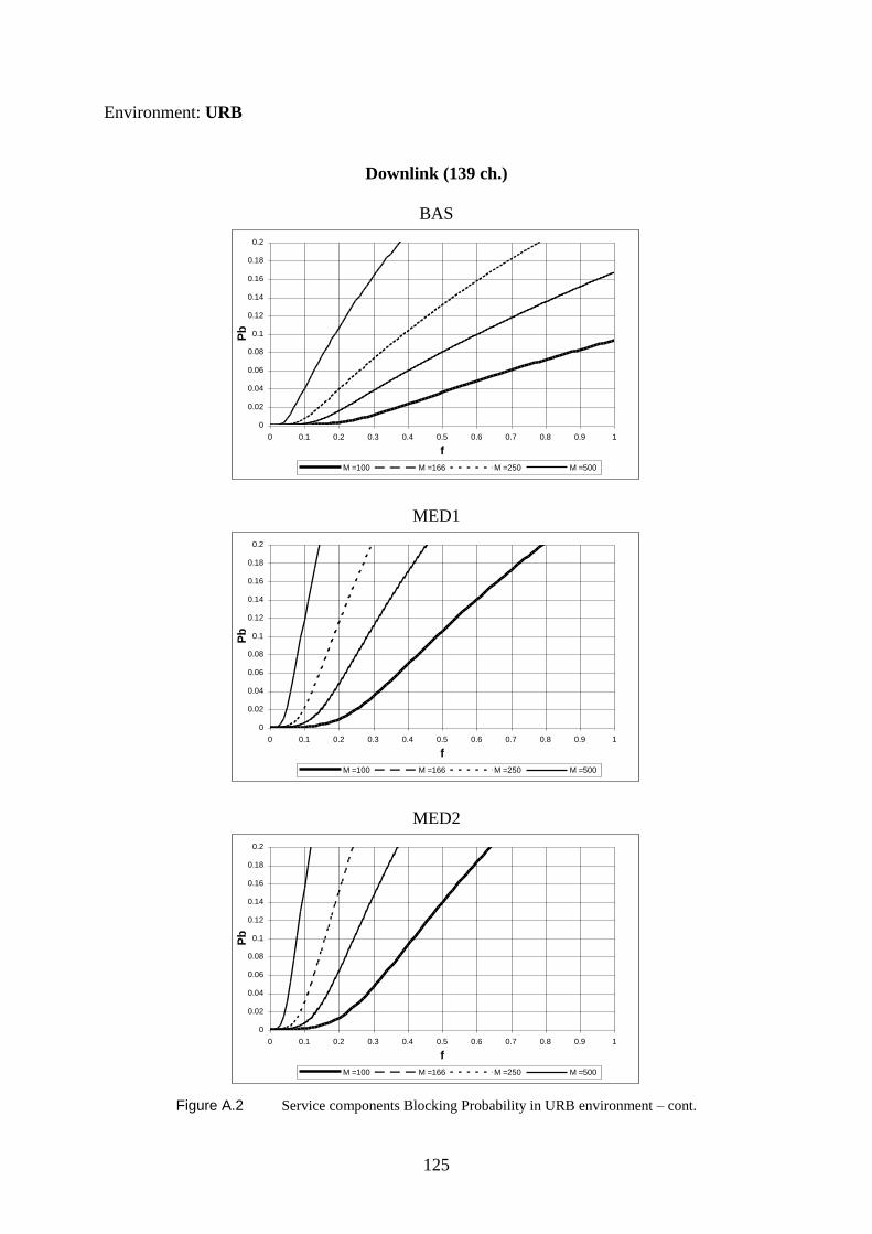
125
Environment: URB
Downlink (139 ch.)
BAS
0
0.02
0.04
0.06
0.08
0.1
0.12
0.14
0.16
0.18
0.2
0 0.1 0.2 0.3 0.4 0.5 0.6 0.7 0.8 0.9 1
f
Pb
M =100 M =166 M =250 M =500
MED1
0
0.02
0.04
0.06
0.08
0.1
0.12
0.14
0.16
0.18
0.2
0 0.1 0.2 0.3 0.4 0.5 0.6 0.7 0.8 0.9 1
f
Pb
M =100 M =166 M =250 M =500
MED2
0
0.02
0.04
0.06
0.08
0.1
0.12
0.14
0.16
0.18
0.2
0 0.1 0.2 0.3 0.4 0.5 0.6 0.7 0.8 0.9 1
f
Pb
M =100 M =166 M =250 M =500
Figure A.2 Service components Blocking Probability in URB environment – cont.
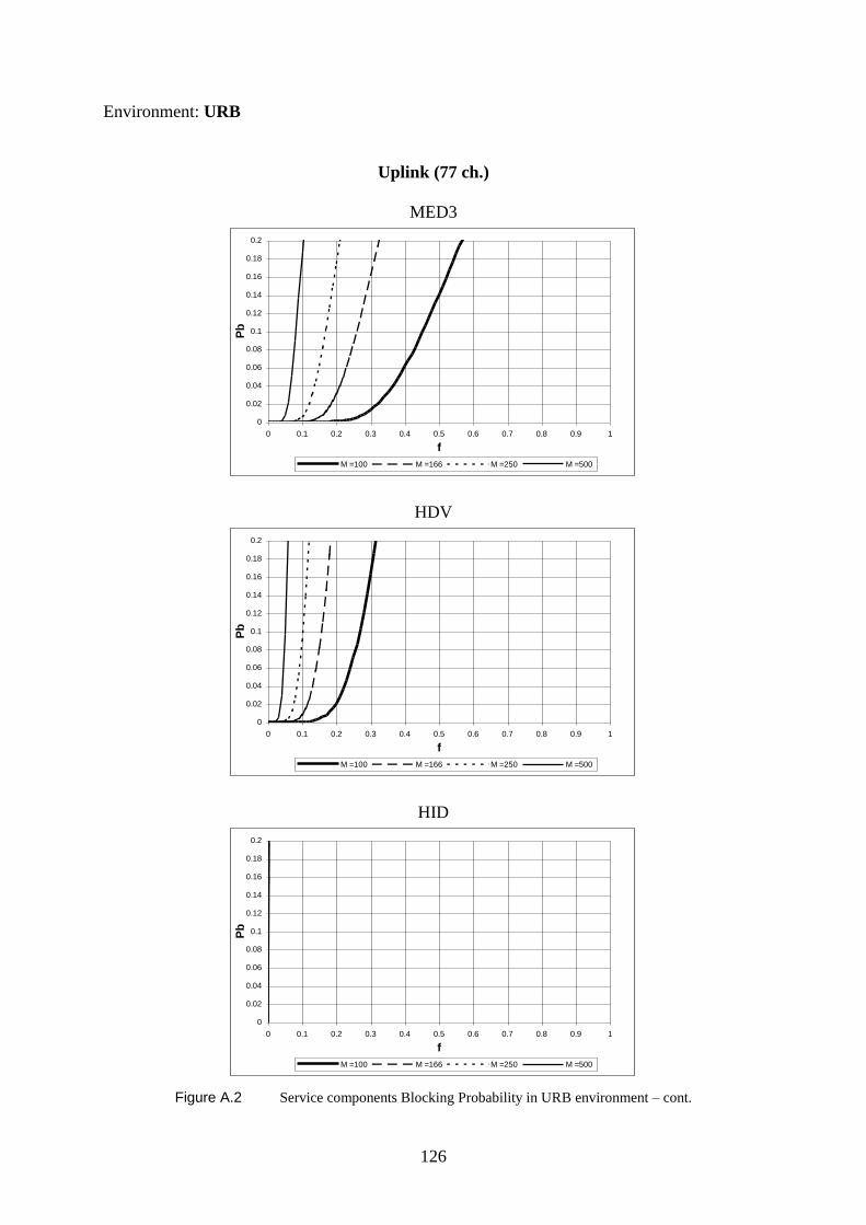
126
Environment: URB
Uplink (77 ch.)
MED3
0
0.02
0.04
0.06
0.08
0.1
0.12
0.14
0.16
0.18
0.2
0 0.1 0.2 0.3 0.4 0.5 0.6 0.7 0.8 0.9 1
f
Pb
M =100 M =166 M =250 M =500
HDV
0
0.02
0.04
0.06
0.08
0.1
0.12
0.14
0.16
0.18
0.2
0 0.1 0.2 0.3 0.4 0.5 0.6 0.7 0.8 0.9 1
f
Pb
M =100 M =166 M =250 M =500
HID
0
0.02
0.04
0.06
0.08
0.1
0.12
0.14
0.16
0.18
0.2
0 0.1 0.2 0.3 0.4 0.5 0.6 0.7 0.8 0.9 1
f
Pb
M =100 M =166 M =250 M =500
Figure A.2 Service components Blocking Probability in URB environment – cont.
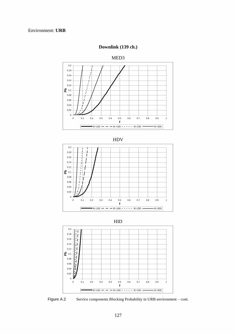
127
Environment: URB
Downlink (139 ch.)
MED3
0
0.02
0.04
0.06
0.08
0.1
0.12
0.14
0.16
0.18
0.2
0 0.1 0.2 0.3 0.4 0.5 0.6 0.7 0.8 0.9 1
f
Pb
M =100 M =166 M =250 M =500
HDV
0
0.02
0.04
0.06
0.08
0.1
0.12
0.14
0.16
0.18
0.2
0 0.1 0.2 0.3 0.4 0.5 0.6 0.7 0.8 0.9 1
f
Pb
M =100 M =166 M =250 M =500
HID
0
0.02
0.04
0.06
0.08
0.1
0.12
0.14
0.16
0.18
0.2
0 0.1 0.2 0.3 0.4 0.5 0.6 0.7 0.8 0.9 1
f
Pb
M =100 M =166 M =250 M =500
Figure A.2 Service components Blocking Probability in URB environment – cont.
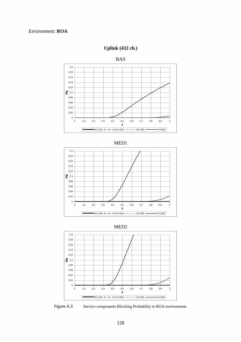
128
Environment: ROA
Uplink (432 ch.)
BAS
0
0.02
0.04
0.06
0.08
0.1
0.12
0.14
0.16
0.18
0.2
0 0.1 0.2 0.3 0.4 0.5 0.6 0.7 0.8 0.9 1
f
Pb
M =100 M =166 M =250 M =500
MED1
0
0.02
0.04
0.06
0.08
0.1
0.12
0.14
0.16
0.18
0.2
0 0.1 0.2 0.3 0.4 0.5 0.6 0.7 0.8 0.9 1
f
Pb
M =100 M =166 M =250 M =500
MED2
0
0.02
0.04
0.06
0.08
0.1
0.12
0.14
0.16
0.18
0.2
0 0.1 0.2 0.3 0.4 0.5 0.6 0.7 0.8 0.9 1
f
Pb
M =100 M =166 M =250 M =500
Figure A.3 Service components Blocking Probability in ROA environment.
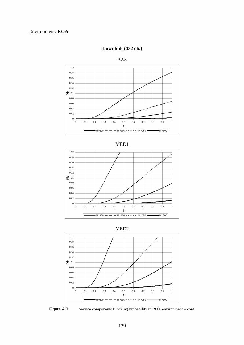
129
Environment: ROA
Downlink (432 ch.)
BAS
0
0.02
0.04
0.06
0.08
0.1
0.12
0.14
0.16
0.18
0.2
0 0.1 0.2 0.3 0.4 0.5 0.6 0.7 0.8 0.9 1
f
Pb
M =100 M =166 M =250 M =500
MED1
0
0.02
0.04
0.06
0.08
0.1
0.12
0.14
0.16
0.18
0.2
0 0.1 0.2 0.3 0.4 0.5 0.6 0.7 0.8 0.9 1
f
Pb
M =100 M =166 M =250 M =500
MED2
0
0.02
0.04
0.06
0.08
0.1
0.12
0.14
0.16
0.18
0.2
0 0.1 0.2 0.3 0.4 0.5 0.6 0.7 0.8 0.9 1
f
Pb
M =100 M =166 M =250 M =500
Figure A.3 Service components Blocking Probability in ROA environment – cont.
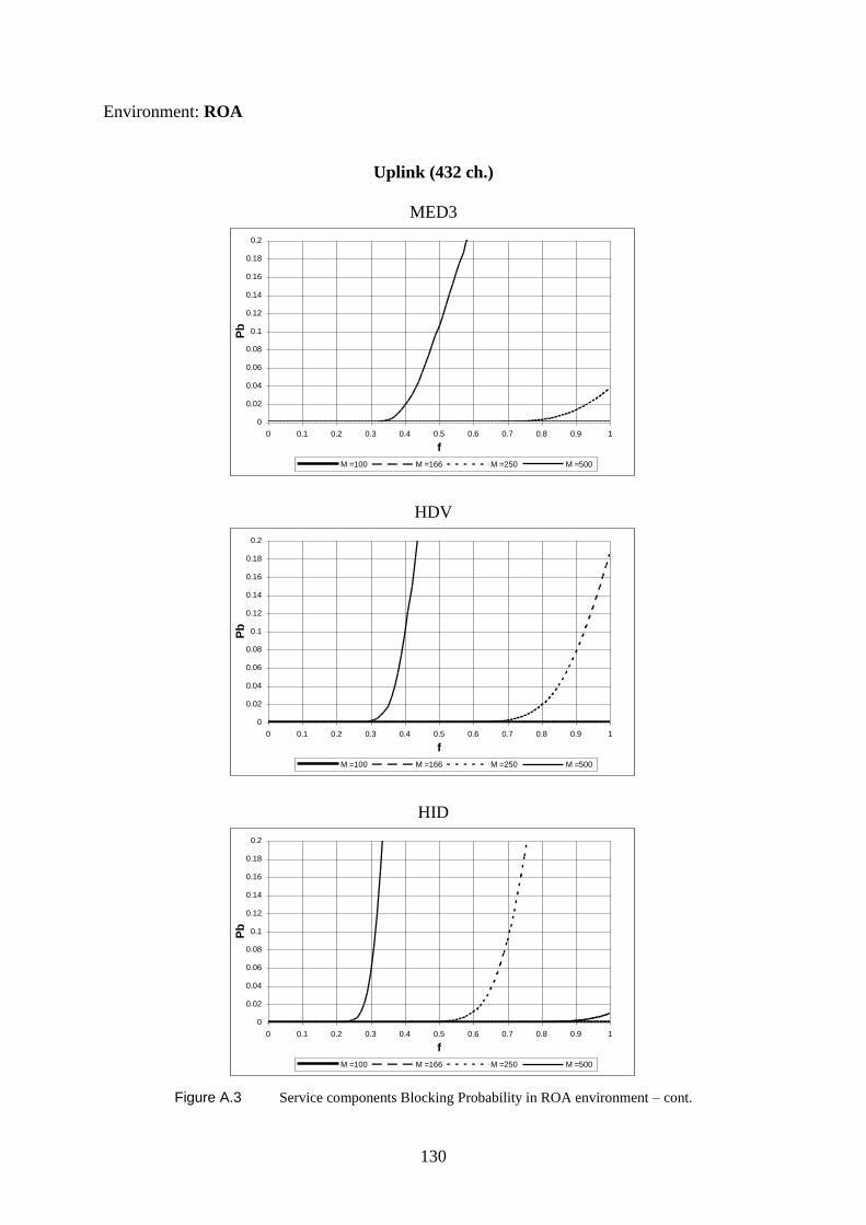
130
Environment: ROA
Uplink (432 ch.)
MED3
0
0.02
0.04
0.06
0.08
0.1
0.12
0.14
0.16
0.18
0.2
0 0.1 0.2 0.3 0.4 0.5 0.6 0.7 0.8 0.9 1
f
Pb
M =100 M =166 M =250 M =500
HDV
0
0.02
0.04
0.06
0.08
0.1
0.12
0.14
0.16
0.18
0.2
0 0.1 0.2 0.3 0.4 0.5 0.6 0.7 0.8 0.9 1
f
Pb
M =100 M =166 M =250 M =500
HID
0
0.02
0.04
0.06
0.08
0.1
0.12
0.14
0.16
0.18
0.2
0 0.1 0.2 0.3 0.4 0.5 0.6 0.7 0.8 0.9 1
f
Pb
M =100 M =166 M =250 M =500
Figure A.3 Service components Blocking Probability in ROA environment – cont.
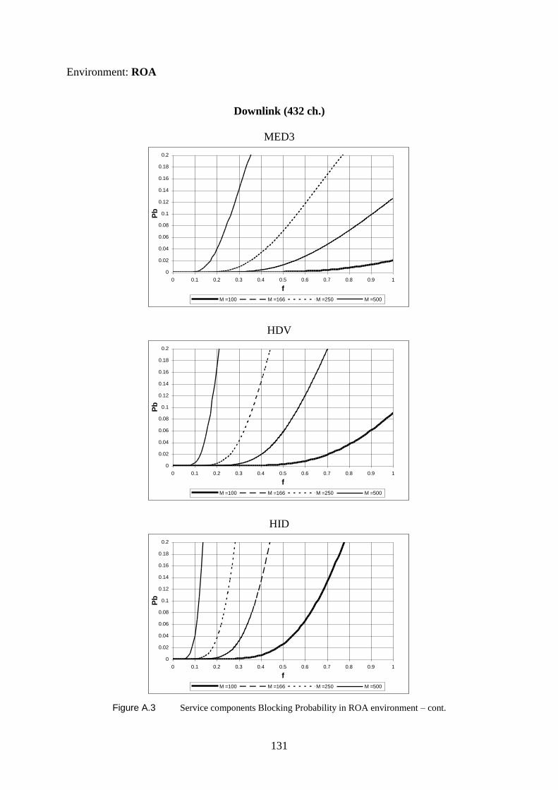
131
Environment: ROA
Downlink (432 ch.)
MED3
0
0.02
0.04
0.06
0.08
0.1
0.12
0.14
0.16
0.18
0.2
0 0.1 0.2 0.3 0.4 0.5 0.6 0.7 0.8 0.9 1
f
Pb
M =100 M =166 M =250 M =500
HDV
0
0.02
0.04
0.06
0.08
0.1
0.12
0.14
0.16
0.18
0.2
0 0.1 0.2 0.3 0.4 0.5 0.6 0.7 0.8 0.9 1
f
Pb
M =100 M =166 M =250 M =500
HID
0
0.02
0.04
0.06
0.08
0.1
0.12
0.14
0.16
0.18
0.2
0 0.1 0.2 0.3 0.4 0.5 0.6 0.7 0.8 0.9 1
f
Pb
M =100 M =166 M =250 M =500
Figure A.3 Service components Blocking Probability in ROA environment – cont.

132
Environment: ROA
Uplink (108 ch.)
BAS
0
0.02
0.04
0.06
0.08
0.1
0.12
0.14
0.16
0.18
0.2
0 0.1 0.2 0.3 0.4 0.5 0.6 0.7 0.8 0.9 1
f
Pb
M =100 M =166 M =250 M =500
MED1
0
0.02
0.04
0.06
0.08
0.1
0.12
0.14
0.16
0.18
0.2
0 0.1 0.2 0.3 0.4 0.5 0.6 0.7 0.8 0.9 1
f
Pb
M =100 M =166 M =250 M =500
MED2
0
0.02
0.04
0.06
0.08
0.1
0.12
0.14
0.16
0.18
0.2
0 0.1 0.2 0.3 0.4 0.5 0.6 0.7 0.8 0.9 1
f
Pb
M =100 M =166 M =250 M =500
Figure A.3 Service components Blocking Probability in ROA environment – cont.

133
Environment: ROA
Downlink (108 ch.)
BAS
0
0.02
0.04
0.06
0.08
0.1
0.12
0.14
0.16
0.18
0.2
0 0.1 0.2 0.3 0.4 0.5 0.6 0.7 0.8 0.9 1
f
Pb
M =100 M =166 M =250 M =500
MED1
0
0.02
0.04
0.06
0.08
0.1
0.12
0.14
0.16
0.18
0.2
0 0.1 0.2 0.3 0.4 0.5 0.6 0.7 0.8 0.9 1
f
Pb
M =100 M =166 M =250 M =500
MED2
0
0.02
0.04
0.06
0.08
0.1
0.12
0.14
0.16
0.18
0.2
0 0.1 0.2 0.3 0.4 0.5 0.6 0.7 0.8 0.9 1
f
Pb
M =100 M =166 M =250 M =500
Figure A.3 Service components Blocking Probability in ROA environment – cont.

134
Environment ROA
Uplink (108 ch.)
MED3
0
0.02
0.04
0.06
0.08
0.1
0.12
0.14
0.16
0.18
0.2
0 0.1 0.2 0.3 0.4 0.5 0.6 0.7 0.8 0.9 1
f
Pb
M =100 M =166 M =250 M =500
HDV
0
0.02
0.04
0.06
0.08
0.1
0.12
0.14
0.16
0.18
0.2
0 0.1 0.2 0.3 0.4 0.5 0.6 0.7 0.8 0.9 1
f
Pb
M =100 M =166 M =250 M =500
HID
0
0.02
0.04
0.06
0.08
0.1
0.12
0.14
0.16
0.18
0.2
0 0.1 0.2 0.3 0.4 0.5 0.6 0.7 0.8 0.9 1
f
Pb
M =100 M =166 M =250 M =500
Figure A.3 Service components Blocking Probability in ROA environment – cont.

135
Environment: ROA
Uplink (85 ch.)
BAS
0
0.02
0.04
0.06
0.08
0.1
0.12
0.14
0.16
0.18
0.2
0 0.1 0.2 0.3 0.4 0.5 0.6 0.7 0.8 0.9 1
f
Pb
M =100 M =166 M =250 M =500
MED1
0
0.02
0.04
0.06
0.08
0.1
0.12
0.14
0.16
0.18
0.2
0 0.1 0.2 0.3 0.4 0.5 0.6 0.7 0.8 0.9 1
f
Pb
M =100 M =166 M =250 M =500
MED2
0
0.02
0.04
0.06
0.08
0.1
0.12
0.14
0.16
0.18
0.2
0 0.1 0.2 0.3 0.4 0.5 0.6 0.7 0.8 0.9 1
f
Pb
M =100 M =166 M =250 M =500
Figure A.3 Service components Blocking Probability in ROA environment – cont.

136
Environment: ROA
Downlink (131 ch.)
BAS
0
0.02
0.04
0.06
0.08
0.1
0.12
0.14
0.16
0.18
0.2
0 0.1 0.2 0.3 0.4 0.5 0.6 0.7 0.8 0.9 1
f
Pb
M =100 M =166 M =250 M =500
MED1
0
0.02
0.04
0.06
0.08
0.1
0.12
0.14
0.16
0.18
0.2
0 0.1 0.2 0.3 0.4 0.5 0.6 0.7 0.8 0.9 1
f
Pb
M =100 M =166 M =250 M =500
MED2
0
0.02
0.04
0.06
0.08
0.1
0.12
0.14
0.16
0.18
0.2
0 0.1 0.2 0.3 0.4 0.5 0.6 0.7 0.8 0.9 1
f
Pb
M =100 M =166 M =250 M =500
Figure A.3 Service components Blocking Probability in ROA environment – cont.
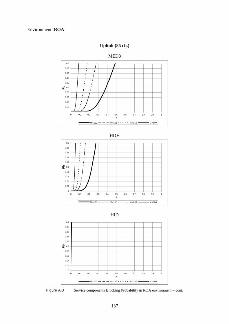
137
Environment: ROA
Uplink (85 ch.)
MED3
0
0.02
0.04
0.06
0.08
0.1
0.12
0.14
0.16
0.18
0.2
0 0.1 0.2 0.3 0.4 0.5 0.6 0.7 0.8 0.9 1
f
Pb
M =100 M =166 M =250 M =500
HDV
0
0.02
0.04
0.06
0.08
0.1
0.12
0.14
0.16
0.18
0.2
0 0.1 0.2 0.3 0.4 0.5 0.6 0.7 0.8 0.9 1
f
Pb
M =100 M =166 M =250 M =500
HID
0
0.02
0.04
0.06
0.08
0.1
0.12
0.14
0.16
0.18
0.2
0 0.1 0.2 0.3 0.4 0.5 0.6 0.7 0.8 0.9 1
f
Pb
M =100 M =166 M =250 M =500
Figure A.3 Service components Blocking Probability in ROA environment – cont.

138
Environment: ROA
Downlink (131 ch.)
MED3
0
0.02
0.04
0.06
0.08
0.1
0.12
0.14
0.16
0.18
0.2
0 0.1 0.2 0.3 0.4 0.5 0.6 0.7 0.8 0.9 1
f
Pb
M =100 M =166 M =250 M =500
HDV
0
0.02
0.04
0.06
0.08
0.1
0.12
0.14
0.16
0.18
0.2
0 0.1 0.2 0.3 0.4 0.5 0.6 0.7 0.8 0.9 1
f
Pb
M =100 M =166 M =250 M =500
HID
0
0.02
0.04
0.06
0.08
0.1
0.12
0.14
0.16
0.18
0.2
0 0.1 0.2 0.3 0.4 0.5 0.6 0.7 0.8 0.9 1
f
Pb
M =100 M =166 M =250 M =500
Figure A.3 Service components Blocking Probability in ROA environment – cont.
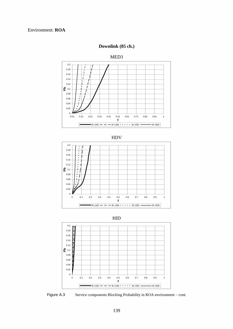
139
Environment: ROA
Downlink (85 ch.)
MED3
0
0.02
0.04
0.06
0.08
0.1
0.12
0.14
0.16
0.18
0.2
0.01 0.11 0.21 0.31 0.41 0.51 0.61 0.71 0.81 0.91 1
f
Pb
M =100 M =166 M =250 M =500
HDV
0
0.02
0.04
0.06
0.08
0.1
0.12
0.14
0.16
0.18
0.2
0 0.1 0.2 0.3 0.4 0.5 0.6 0.7 0.8 0.9 1
f
Pb
M =100 M =166 M =250 M =500
HID
0
0.02
0.04
0.06
0.08
0.1
0.12
0.14
0.16
0.18
0.2
0 0.1 0.2 0.3 0.4 0.5 0.6 0.7 0.8 0.9 1
f
Pb
M =100 M =166 M =250 M =500
Figure A.3 Service components Blocking Probability in ROA environment – cont.

140
141
References
[Adas97] A. Adas, "Traffic Models in Broadband Networks" IEEE Communications
Magazine, Jul. 1997, pp. 82-89.
[AdZu98] R.G. Addie, M. Zukerman and T.D. Neame, "Broadband Traffic Modelling:
Simple Solutions to Hard Problems," IEEE Communications Magazine, Vol.
36, No. 8, Aug. 1998, pp. 88-95.
[AwVl96] G.A.Awater and H.A.van de Vlag, "Exact Computation of Time and Call
Blocking Probabilities in Large, Multi-traffic, Multi-resource Loss Systems,"
Performance Evaluation, Vol. 25, Mar. 1996, pp.41-58.
[Beck00] F. Beckman "General Mobile Internet Market Requirements on the
development of Services for UMTS/WCDMA", Ericsson Internal
Documentation, No ERA/GG-00:0019.
[BuCN99] D. Bull, N. Canagarajah and A. Nix, Insights into Mobile Multimedia
Communications, Academic Press, New York, NY, USA, 1999.
[CoPr97] L.M. Correia, R. Prasad "An Overview of Wireless Broadband
Communications", IEEE Communications Magazine, Jul. 1997, pp. 28-33.
[DuSm94] J. Dunlop and D.G. Smith, Telecommunications Engineering, Chapman and
Hall, London, UK, 1994.
[EN1399] [EN/LZT 123 4613 R1B] Ericsson Student Text "WCDMA Experimental
System Survey", Ericsson Radio systems AB, 1999.
[EN7499] EN/LZT 123 5374 R1B Ericsson Student Text "GPRS System Survey",
Ericsson Radio systems AB, 1999.
[FrMe94] V.S.Frost and B.Melamed, "Traffic Modeling For Telecommunications
Networks," IEEE Communications Magazine, Vol. 32, No. 3, Mar. 1994, pp.
70-81.
[Hill79] M.T. Hills, "Telecommunications Switching Principles" George allen &
UNWIN, London 1979.
[HoRa86] D. Hong and T.S. Rappaport, "Traffic Model and Performance Analysis for
Cellular Mobile Radio Telephone Systems with Prioritized and Non-prioritized
Hand-off Procedures," IEEE Transactions on Vehicular Technology, Vol. VT-
35, No. 3, Aug. 1986, pp.77-92.
142
[Jabb96] B. Jabbari, "Teletraffic Aspects of Evolving and Next-Generation Wireless
Communication Networks," IEEE Personal Communications Magazine, Vol.
3, No. 6, Dec. 1996, pp. 4-9.
[KeLi99] K.Kennedy and R.Litjens, "Performance Evaluation Of A Hybrid Radio
Resource Allocation Algorithm In A GSM/GPRS Network," in Proc. of
PIMRC'99 – 10th
IEEE International Symposium on Personal Indoor and
Mobile Radio Communications, Osaka, Japan, Sep. 1999.
[Klei76] L. Kleinrock, Queuing Systems, Wiley-Interscience, Chichester, Sussex, UK,
1976.
[Kwok95] T. Kwok, "A vision for Residential Broadband Services: ATM to the home",
IEEE Network, Vol. 9, No. 5, Sep/Oct. 1995, pp. 14-28.
[Kwok97] T. Kwok, "Residential Broadband Internet Servicess and Applications
Requirements, IEEE Communications Magazine, Vol. 35, No. 7, Jul. 1997, pp.
76-83.
[Mino93] D. Minoli, "Enterprise Networking: Fractional T1 to Sonet, Frame Relay to
BISDN", Artech House, Norwood, 1993.
[MMMM98] M.A. Marsan, S. Marano, C.Mastroianni and M.Meo, "Performance Analysis
of Cellular Mobile Communication Networks Supporting Multimedia
Services," in Proc. of 6th
International Symposium on Modeling, Analysis and
Simulation of Computer and Telecommunication Systems, Los Alamitos, CA,
USA, 1998, pp. 274-281.
[NaAc95] M.Naghshined and A.S.Acampora, "QOS Provisioning in Micro-Cellular
Networks Supporting Multimedia Traffic," in Proc. of Infocom'95 – The IEEE
Conference on Computer Communications, Los Alamitos, CA, USA, 1995,
pp.1075-1084.
[NaBK00] S.Nanda and K. Balachandran, and S.Kumar, "Adaptation Techniques in
Wireless Packet Data Services," IEEE Communications Magazine, Vol. 38, No
1, Jan 2000, pp.54-65.
[Phil87] D.T. Philips, "Operations Research", John Wiley & Sons, Inc 1987
[Pras98] R. Prasad "An Overview of CDMA Evolution Toward Wideband CDMA",
IEEE Communications Surveys, Q4 1998, Vol. 1, no 1.
143
[Rapp96] T.S. Rappaport, Wireless Communications, IEEE Press, Piscataway, NJ, USA,
1996.
[RoPa99] I. Rombogiannakis and M. Paterakis, "Voice /Data Integrated Wireless
Channel Access in Third Generation Digital Cellular Networks: The
Performance of Bursty Data Generated by Interactive Applications,"
International Journal of Wireless Information Networks, Vol. 5, No. 1, 1998,
pp. 1-12.
[Schw97] M. Schwartz, "Telecommunication Networks", Addison-Wesley Publishing
Company, Nov 1987.
[SMRA89] P. Sen, B. Maglaris, N. Rikli, D. Anastassiou "Models for Packed Switching of
Variable-Bit-Rate Video Sources", Journal on Selected Areas in
Telecommunication, vol. 37, no 5, 1989 pp. 865 – 869.
[VeCo98] F. Velez, L.M. Correia, "Capacity Trade-offs in Mobile Broadband Systems
using Guard Channels for High Mobility Handover," in Proc. of PIRC'98 - 9th
IEEE International Symposium on Personal Indoor, and Mobile Radio
Communications, Boston, Massachusetts, USA, Sep. 1998, pp. 749-753.
[VeCo99] F.J.Velez, L.M.Correia, "New Calls Traffic Performance in Micro-cellular
Mobile Broadband Systems with High Mobility Handover", in Proc. of.
ConfTele'99-II Conference on Telecomunications, Sesimbra, Portugal, Apr.
1999.
[VeCo00] F.J.Velez, L.M.Correia, "Multiservice Traffic in Mobile Broadband Systems",
Internal Report, Instituto de Telecomunicacoes, Lisbon, Portugal, Oct. 2000.
[Vele99] F.J. Velez, "Multi-service Traffic Analysis in Mobile Broadband Systems", in
Proc. of 4th
ACTS Mobile Communications Summit, Sorrento, Italy, June 1999,
pp.239-244.
[Wirt97] P.E.Wirth, "The Role of Teletraffic Modelling in the New Communications
Paradigms," IEEE Communications Magazine, Vol. 35, No. 8, Aug. 1997, pp.
86-92.
[Yaco93] M.D. Yacoub, Foundations of Mobile Radio Engineering, CRC Press, Boca
Raton, FL, USA, 1993.