Multiscale modelling of nanomechanics and …nkioussi/publications/2003PhilMag.Review.pdfMultiscale modelling of nanomechanics and micromechanics: an overview ... (MMM) approaches

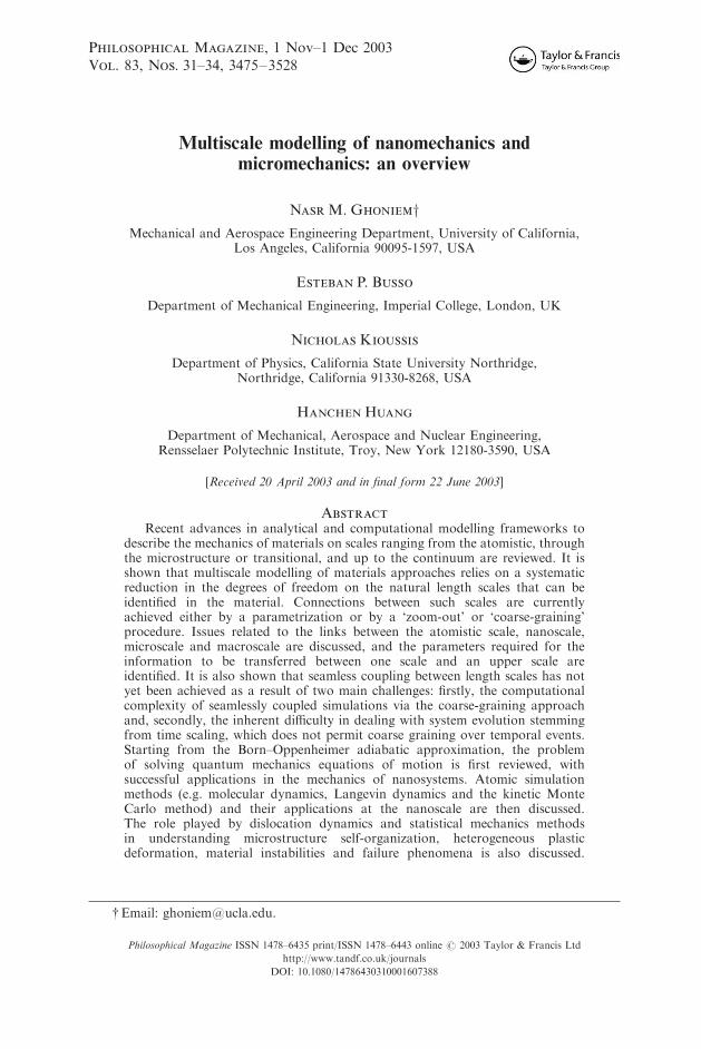
Philosophical Magazine, 1 Nov–1 Dec 2003Vol. 83, Nos. 31–34, 3475–3528

Multiscale modelling of nanomechanics andmicromechanics: an overview

Nasr M. GhoniemyMechanical and Aerospace Engineering Department, University of California,

Los Angeles, California 90095-1597, USA

Esteban P. Busso

Department of Mechanical Engineering, Imperial College, London, UK

Nicholas Kioussis

Department of Physics, California State University Northridge,Northridge, California 91330-8268, USA

Hanchen Huang

Department of Mechanical, Aerospace and Nuclear Engineering,Rensselaer Polytechnic Institute, Troy, New York 12180-3590, USA

[Received 20 April 2003 and in final form 22 June 2003]

Abstract

Recent advances in analytical and computational modelling frameworks todescribe the mechanics of materials on scales ranging from the atomistic, throughthe microstructure or transitional, and up to the continuum are reviewed. It isshown that multiscale modelling of materials approaches relies on a systematicreduction in the degrees of freedom on the natural length scales that can beidentified in the material. Connections between such scales are currentlyachieved either by a parametrization or by a ‘zoom-out’ or ‘coarse-graining’procedure. Issues related to the links between the atomistic scale, nanoscale,microscale and macroscale are discussed, and the parameters required for theinformation to be transferred between one scale and an upper scale areidentified. It is also shown that seamless coupling between length scales has notyet been achieved as a result of two main challenges: firstly, the computationalcomplexity of seamlessly coupled simulations via the coarse-graining approachand, secondly, the inherent difficulty in dealing with system evolution stemmingfrom time scaling, which does not permit coarse graining over temporal events.Starting from the Born–Oppenheimer adiabatic approximation, the problemof solving quantum mechanics equations of motion is first reviewed, withsuccessful applications in the mechanics of nanosystems. Atomic simulationmethods (e.g. molecular dynamics, Langevin dynamics and the kinetic MonteCarlo method) and their applications at the nanoscale are then discussed.The role played by dislocation dynamics and statistical mechanics methodsin understanding microstructure self-organization, heterogeneous plasticdeformation, material instabilities and failure phenomena is also discussed.

Philosophical Magazine ISSN 1478–6435 print/ISSN 1478–6443 online # 2003 Taylor & Francis Ltd

http://www.tandf.co.uk/journals

DOI: 10.1080/14786430310001607388

yEmail: [email protected].

Finally, we review the main continuum-mechanics-based framework used todayto describe the nonlinear deformation behaviour of materials at the local (e.g.single phase or grain level) and macroscopic (e.g. polycrystal) scales. Emphasis isplaced on recent progress made in crystal plasticity, strain gradient plasticity andhomogenization techniques to link deformation phenomena simultaneouslyoccurring at different scales in the material microstructure with its macroscopicbehaviour. In view of this wide range of descriptions of material phenomenainvolved, the main theoretical and computational difficulties and challenges arecritically assessed.

} 1. Introduction

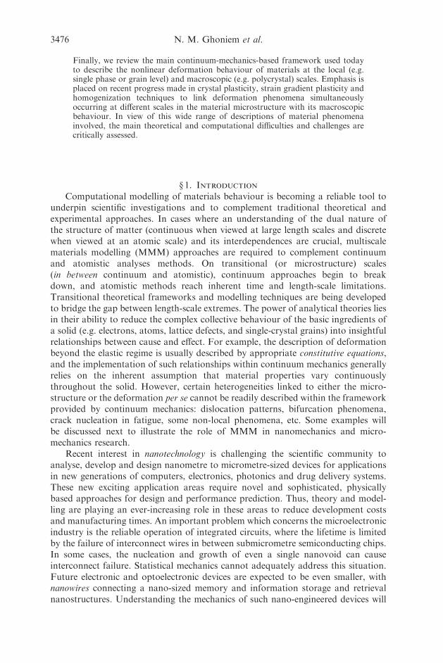
Computational modelling of materials behaviour is becoming a reliable tool tounderpin scientific investigations and to complement traditional theoretical andexperimental approaches. In cases where an understanding of the dual nature ofthe structure of matter (continuous when viewed at large length scales and discretewhen viewed at an atomic scale) and its interdependences are crucial, multiscalematerials modelling (MMM) approaches are required to complement continuumand atomistic analyses methods. On transitional (or microstructure) scales(in between continuum and atomistic), continuum approaches begin to breakdown, and atomistic methods reach inherent time and length-scale limitations.Transitional theoretical frameworks and modelling techniques are being developedto bridge the gap between length-scale extremes. The power of analytical theories liesin their ability to reduce the complex collective behaviour of the basic ingredients ofa solid (e.g. electrons, atoms, lattice defects, and single-crystal grains) into insightfulrelationships between cause and effect. For example, the description of deformationbeyond the elastic regime is usually described by appropriate constitutive equations,and the implementation of such relationships within continuum mechanics generallyrelies on the inherent assumption that material properties vary continuouslythroughout the solid. However, certain heterogeneities linked to either the micro-structure or the deformation per se cannot be readily described within the frameworkprovided by continuum mechanics: dislocation patterns, bifurcation phenomena,crack nucleation in fatigue, some non-local phenomena, etc. Some examples willbe discussed next to illustrate the role of MMM in nanomechanics and micro-mechanics research.

Recent interest in nanotechnology is challenging the scientific community toanalyse, develop and design nanometre to micrometre-sized devices for applicationsin new generations of computers, electronics, photonics and drug delivery systems.These new exciting application areas require novel and sophisticated, physicallybased approaches for design and performance prediction. Thus, theory and model-ling are playing an ever-increasing role in these areas to reduce development costsand manufacturing times. An important problem which concerns the microelectronicindustry is the reliable operation of integrated circuits, where the lifetime is limitedby the failure of interconnect wires in between submicrometre semiconducting chips.In some cases, the nucleation and growth of even a single nanovoid can causeinterconnect failure. Statistical mechanics cannot adequately address this situation.Future electronic and optoelectronic devices are expected to be even smaller, withnanowires connecting a nano-sized memory and information storage and retrievalnanostructures. Understanding the mechanics of such nano-engineered devices will

3476 N. M. Ghoniem et al.

enable high levels of reliability and useful lifetimes to be achieved. Undoubtedly,defects are expected to play a major role in these nanosystems and microsystemsowing to the crucial impact on the physical and mechanical performance.

The potential of MMM approaches for computational materials design is alsogreat. Such possibility was recently illustrated on a six-component Ti-based alloy,with a composition predetermined by electronic properties, which was shown toexhibit an entirely new twin- and dislocation-free deformation mechanism, leadingto ‘unexpected new properties, such as high ductility and strength, and Invar andElinvar behaviour’ (Saito et al. 2003). Such an alloy would be unlikely to be found bytrial and error. This points to a paradigm shift in modelling, away from reproducingknown properties of known materials and towards simulating the behaviour ofpossible alloys as a forerunner to finding real materials with these properties.

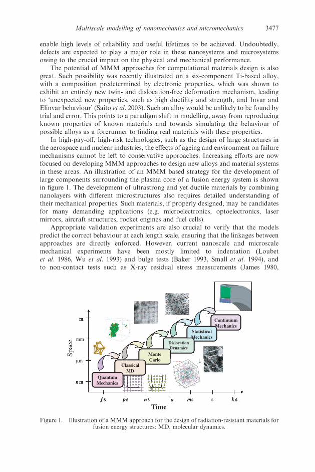
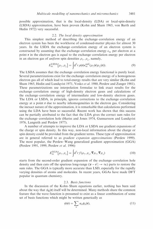
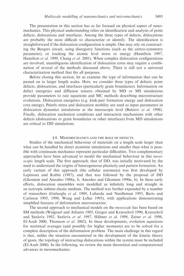
In high-pay-off, high-risk technologies, such as the design of large structures inthe aerospace and nuclear industries, the effects of ageing and environment on failuremechanisms cannot be left to conservative approaches. Increasing efforts are nowfocused on developing MMM approaches to design new alloys and material systemsin these areas. An illustration of an MMM based strategy for the development oflarge components surrounding the plasma core of a fusion energy system is shownin figure 1. The development of ultrastrong and yet ductile materials by combiningnanolayers with different microstructures also requires detailed understanding oftheir mechanical properties. Such materials, if properly designed, may be candidatesfor many demanding applications (e.g. microelectronics, optoelectronics, lasermirrors, aircraft structures, rocket engines and fuel cells).

Appropriate validation experiments are also crucial to verify that the modelspredict the correct behaviour at each length scale, ensuring that the linkages betweenapproaches are directly enforced. However, current nanoscale and microscalemechanical experiments have been mostly limited to indentation (Loubetet al. 1986, Wu et al. 1993) and bulge tests (Baker 1993, Small et al. 1994), andto non-contact tests such as X-ray residual stress measurements (James 1980,

Multiscale modelling of nanomechanics and micromechanics 3477

ContinuumMechanics

StatisticalMechanics

DislocationDynamics

p sf s n s s m k s

n m

m

MonteCarlo

ClassicalMD

QuantumMechanics

3

S

3

S

b

0

1000

2000

3000

4000

5000

z(a)

0

1000

2000

3000

4000

5000

x(a)

0

1000

2000

3000

4000

5000

y(a)

X Y

Z

σ = 165 Mpa

ContinuumMechanics


DislocationDynamics

p sf s n s s m k s

n m

m

MonteCarlo

ClassicalMD

QuantumMechanics

3

S

3

S

b

0

1000

2000

3000

4000

5000

z(a)

0

1000

2000

3000

4000

5000

x(a)

0

1000

2000

3000

4000

5000

y(a)

X Y

Z

σ = 165 Mpa

ContinuumMechanics


DislocationDynamics

p sf s n s s m k s

n m

m

MonteCarlo

ClassicalMD

QuantumMechanics

ContinuumMechanics


DislocationDynamics

p sf s n s s ms s k s

Time

n m

m

MonteCarlo

ClassicalMD

QuantumMechanics

3

S

3

S

b

0

1000

2000

3000

4000

5000

z(a)

0

1000

2000

3000

4000

5000

x(a)

0

1000

2000

3000

4000

5000

y(a)

X Y

Z

σ = 165 Mpaµm

mm

Spac

e

Figure 1. Illustration of a MMM approach for the design of radiation-resistant materials forfusion energy structures: MD, molecular dynamics.

Segmueller and Murakami 1988). Multiscale interconnected approaches will need tobe developed to interpret new and highly specialized nanomechanical and micro-mechanical tests. One of the advantages of these approaches is that, at each stage,physically meaningful parameters are predicted and used in subsequent models,avoiding the use of empiricism and fitting parameters.

As the material dimensions become smaller, its resistance to deformation isincreasingly determined by internal or external discontinuities (e.g. surfaces, grainboundaries and dislocation cell walls). The Hall–Petch relationship has been widelyused to explain grain-size effects, although the basis of the relationship is strictlyrelated to dislocation pile-ups at grain boundaries. Recent experimental observationson nanocrystalline materials with grains of the order of 10–20 nm indicate thatthe material is weaker than would be expected from the Hall–Petch relationship(Erb et al. 1996, Campbell et al. 1998). Thus, the interplay between interfacial orgrain-boundary effects and slip mechanisms within a single-crystal grain may resultin either strength or weakness, depending on their relative sizes. Although experi-mental observations of plastic deformation heterogeneities are not new, the signifi-cance of these observations has not been addressed until very recently. In the samemetallic alloys, regular patterns of highly localized deformation zones, surroundedby vast material volumes which contain little or no deformation, are frequently seen(Mughrabi 1983, 1987, Amodeo and Ghoniem 1988). The length scale associatedwith these patterns (e.g. typically the size of dislocation cells, the ladder spacingin persistent slip bands (PSBs) or the spacing between coarse shear bands) controlsthe material strength and ductility. As it may not be possible to homogenize suchtypes of microstructure in an average sense using either atomistic simulations orcontinuum theories, new intermediate approaches will be needed.

The issues discussed above, in addition to the ever-increasingly powerfuland sophisticated computer hardware and software available, are driving thedevelopment of MMM approaches in nanomechanics and micromechanics. It isexpected that, within the next decade, new concepts, theories and computationaltools will be developed to make truly seamless multiscale modelling a reality.In this overview article, we briefly outline the status of research in each componentthat makes up the MMM paradigm for modelling nanosystems and microsystems:quantum mechanics (QM), molecular dynamics (MD), Monte Carlo (MC) method,dislocation dynamics (DD), statistical mechanics (SM) and, finally, continuummechanics (CM).

} 2. Computational quantum mechanics

2.1. Essential conceptsThere is little doubt that most of the low-energy physics, chemistry, materials

science and biology can be explained by the QM of electrons and ions and that,in many cases, the properties and behaviour of materials derive from the quantum-mechanical description of events at the atomic scale. Although there are manyexamples in materials science of significant progress having been made withoutany need for quantum-mechanical modelling, this progress is often limited as onepushes forward and encounters the atomic world. For instance, the understanding ofthe properties of dislocations comes from classical elasticity theory, but even in thesecases, until recently, very little was known about the core of a dislocation or theeffect of chemistry on the core, precisely because this part of the dislocation requires


detailed quantum-mechanical modelling. The ability of QM to predict the totalenergy and the atomic structure of a system of electrons and nuclei enables one toreap a tremendous benefit from a quantum-mechanical calculation. Many methodshave been developed for solving the Schrodinger equation that can be used tocalculate a wide range of physical properties of materials, which require only aspecification of the ions present (by their atomic number). These methods are usuallyreferred to as ab initio methods.

In considering the motion of electrons in condensed matter, we are dealing withthe problem of describing the motion of an enormous number of electrons and nuclei(about 1023) obeying the laws of QM. Prediction of the electronic and geometricstructure of a solid requires calculation of the quantum-mechanical total energy ofthe system and subsequent minimization of that energy with respect to the electronicand nuclear coordinates. Because of the large difference between the masses ofelectrons and nuclei and the fact that the forces on the particles are the same, theelectrons respond essentially instantaneously to the motion of the nuclei. Thus, thenuclei can be treated adiabatically, leading to a separation of the electronic andnuclear coordinates in the many-body wave function

ðfRI, rngÞ ¼ elðfrng; fRIgÞ nucðfRIgÞ, ð1Þ

which is the so-called Born–Oppenheimer approximation (Parr and Yang 1989,Dreizler and Gross 1990). The adiabatic principle reduces the many-body problemin the solution of the dynamics of the electrons in some frozen-in configuration {RI}of the nuclei; this is an example of the philosophy behind systematic degree-of-freedom elimination which is itself at the heart of multiscale modelling.

Even with this simplification, the many-body problem remains formidable. TheHamiltonian for the N-electron system moving in condensed matter with fixed nucleiis (in atomic units)

H ¼XNi¼1

�12=2

i þXNi¼1

v�i ðriÞ þ12

Xi

Xj 6¼i

1

jri � rjj, ð2Þ

where the first term is the kinetic energy operator, v�ðrÞ is the one-electron spin-dependent external potential (e.g. the electron–nucleus interaction), and the thirdterm represents the effect of the electron–electron interactions which poses the mostdifficult problem in any electronic structure calculation.

Density functional theory (DFT) (Hohenberg and Kohn 1964, Kohn andSham 1965, Jones and Gunnarsson 1989, Parr and Yang 1989, Dreizler and Gross1990) has been proven to be a very powerful quantum-mechanical method ininvestigating the electronic structure of atoms, molecules and solids. Here, theelectron density �ðrÞ, or spin density ��ðrÞ, is the fundamental quantity, ratherthan the total wave function employed for example in Hartree–Fock theory(Ashcroft and Mermin 1976). The DFT makes successful predictions of ground-state properties for moderately correlated electronic systems (Perdew 1999). DFTcan provide accurate ground-state properties for real materials (such as total energiesand energy differences, cohesive energies of solids and atomization energies of mole-cules, surface energies, energy barriers, atomic structure, and magnetic moments)and provides a scheme for calculating them (Jones and Gunnarsson 1989, Fulde1993, Perdew 1999).


We next give a brief discussion of the essential concepts of DFT. Hohenberg andKohn (1964) proved that the total energy, including exchange and correlation, of anelectron gas (even in the presence of a static external potential) is a unique functionalof the electron density. The minimum value of the total-energy functional is theground-state energy of the system, and the density that yields this minimum valueis the exact single-particle ground-state density. Kohn and Sham (1965) then showedhow it is possible, formally, to replace the many-electron problem by an exactlyequivalent set of self-consistent one-electron equations

�12=

2þ v�ðrÞ þ

ðd3r0

�ðr0Þ

jr� r0jþ v�xcðrÞ

� � k�ðrÞ ¼ �k� k�ðrÞ, ð3Þ

where k�ðrÞ are the Kohn–Sham orbitals, and the spin-dependent exchange–correlation potential is defined as

v�xcðrÞ �dExc½�", �#�

d��ðrÞ: ð4Þ

Here, Exc½�", �#� is the exchange–correlation energy and the density ��ðrÞ of electronsof spin �(¼ " , #) is found by summing the squares of the occupied orbitals:

��ðrÞ ¼Xk

j k�ðrÞj2�ð�� k�Þ, ð5Þ

where �ðxÞ is the step function and � is the chemical potential. The exchange–correlation energy is ‘nature’s glue’. It is largely responsible for the binding ofatoms to form molecules and solids. The total electronic density is

�ðrÞ ¼ �"ðrÞ þ �#ðrÞ: ð6Þ

Aside from the nucleus–nucleus repulsion energy, the total energy is

E ¼Xk�

h k�j �12=2

j k�i�ð�� k�Þ þX�

ðd3r v�ðrÞ��ðrÞ þU½�� þ Exc½�", �#�, ð7Þ

where

U½�� ¼ 12

ðd3r

ðd3r0

�ðrÞ�ðr0Þ

jr� r0jð8Þ

is the Hartree self-repulsion of the electron density.The Kohn–Sham equations represent a mapping of the interacting many-

electron system on to a system of non-interacting electrons moving in an effectivenon-local potential owing to all the other electrons. The Kohn–Sham equations mustbe solved self-consistently so that the occupied electron states generate a chargedensity that produces the electronic potential that was used to construct theequations. New iterative diagonalization approaches can be used to minimizethe total-energy functional (Car and Parrinello 1985, Gilan 1989, Payne et al.1992). These are much more efficient than the traditional diagonalization methods.If the exchange–correlation energy functional were known exactly, then takingthe functional derivative with respect to the density would produce an exchange–correlation potential that included the effects of exchange and correlation exactly.

The complexity of the real many-body problem is contained in the unknownexchange–correlation potential v�xcðrÞ. Nevertheless, making simple approximations,we can hope to circumvent the complexity of the problem. Indeed the simplest


possible approximation, that is the local-density (LDA) or local-spin-density(LSDA) approximation, have been proven (Kohn and Sham 1965, von Barth andHedin 1972) very successful.

2.2. The local density approximationThis simplest method of describing the exchange–correlation energy of an

electron system has been the workhorse of condensed-matter physics for almost 30years. In the LSDA the exchange–correlation energy of an electron system isconstructed by assuming that the exchange–correlation energy �xc per electron at apoint r in the electron gas is equal to the exchange–correlation energy per electronin an electron gas of uniform spin densities �", �#, namely,

ELSDAxc �", �#

� �¼

ðd3r �ðrÞ�unifxc ð�"ðrÞ�#ðrÞÞ: ð9Þ

The LSDA assumes that the exchange–correlation energy functional is purely local.Several parametrizations exist for the exchange–correlation energy of a homogenouselectron gas all of which lead to total-energy results that are very similar (Kohn andSham 1965, Hedin and Lundqvist 1971, Vosko et al. 1980, Perdew and Zunger 1981).These parametrizations use interpolation formulae to link exact results for theexchange–correlation energy of high-density electron gases and calculations ofthe exchange–correlation energy of intermediate and low-density electron gases.The LDA or LSDA, in principle, ignores corrections to the exchange–correlationenergy at a point r due to nearby inhomogeneities in the electron gas. Consideringthe inexact nature of the approximation, it is remarkable that calculations performedusing the LDA have been so successful. Recent work has shown that this successcan be partially attributed to the fact that the LDA gives the correct sum rules forthe exchange–correlation hole (Hariss and Jones 1974, Gunnarsson and Lundqvist1976, Langreth and Perdew 1977).

A number of attempts to improve the LDA or LSDA use gradient expansions ofthe charge or spin density. In this way, non-local information about the charge orspin density could be provided from the gradient terms. These type of approximationare in general referred to as gradient expansion approximations (Perdew 1999).The most popular, the Perdew–Wang generalized gradient approximation (GGA)(Perdew 1991, 1999, Perdew et al. 1996)

EGGAxc �", �#

� �¼

ðd3r f ð�", �#,=�",=�#Þ ð10Þ

starts from the second-order gradient expansion of the exchange–correlation holedensity and then cuts off the spurious long-range (jr� r

0j ! 1) parts to restore the

sum rules. The GGA is typically more accurate than LSD, especially for the rapidlyvarying densities of atoms and molecules. In recent years, GGAs have made DFTpopular in quantum chemistry.

2.3. Basis functionsIn the discussion of the Kohn–Sham equations earlier, nothing has been said

about the way that kðrÞ itself will be determined. Many methods share the commonfeature that the wave function is presumed to exist as a linear combination of someset of basis functions which might be written generically as

ðrÞ ¼Xn

�n�nðrÞ, ð11Þ


where �n is the weight associated with the nth basis function �nðrÞ. The solution ofthe Kohn–Sham equations in turn becomes a search for unknown coefficients ratherthan unknown functions. Part of the variety associated with the many differentimplementations of DFT codes is associated with the choice of basis functionsand the form of the effective crystal potential. In deciding on a particular set ofbasis functions, a compromise will have to be made between high-accuracy results,which require a large basis set, and computational costs, which favour small basissets. Similar arguments hold with respect to the functional forms of the �nðrÞ. Thereare several powerful techniques in electronic structure calculations. The variousmethods may be divided into those which express the wave functions as linearcombinations of some fixed basis functions, say linear combination of atomicorbitals localized about each atomic site (Eschrig 1989) or those which use afree-electron-like basis, the so-called plane-wave basis set (Payne et al. 1992,Denteneer and van Haeringen 1985). Alternatively, there are those methods whichemploy matching of partial waves, such as the full-potential linear-augmented-plane-wave method (Wimmer et al. 1981), the full-potential linear muffin-tin-orbitalmethod (Price and Cooper 1989, Price et al. 1992) and the full-potentialKorringa–Kohn–Rostoker method (Papanikolaou et al. 2002).

2.4. Nanomechanics applicationsElectronic structure calculations based on DFT also can be applied for studies

of non-periodic systems, such as those containing point, planar or line defects, orquantum dots if a periodic supercell is used. The supercell contains the defect sur-rounded by a region of bulk crystal or vacuum for the case of a surface. Periodicboundary conditions are applied to the supercell so that the supercell is reproducedthroughout space. It is essential to include enough bulk solid (or vacuum) in thesupercell to prevent the defects in neighbouring cells from interacting appreciablywith each other. The independence of defects in neighbouring cells can be checked byincreasing the volume of the supercell until the calculated defect energy is converged.Using the supercell geometry, one can study even molecules (Rappe et al. 1992),provided that the supercell is large enough that the interactions between themolecules are negligible.

The implementation of the DFT within the LDA or the GGA for the exchange–correlation energy, the development of new linearized methods for solving the single-particle Schrodinger equations and the use of powerful computers allow for a highlyefficient treatment of up to several hundreds of atoms and has led to an outburst oftheoretical work in condensed-matter physics and materials physics. Representativesuccessful applications of DFT for a wide variety of materials ranging from metals tosemiconductors to ceramics include the electronic, structural and magnetic proper-ties of surfaces (LaBella et al. 1999, Ruberto et al. 2002), interfaces (Batirev et al.1999), grain boundaries (Wu et al. 1994, Lu et al. 1999, Lu and Kioussis 2001), alloys(Kent and Zunger 2001, Janotti et al. 2002), chemisorption of molecules on surfaces(Durr et al. 2001), C nanotubes (Chan et al. 2001, Yildrim et al. 2001) and quantumdots (Wang et al. 1999). For example, recent ab initio calculations predict that tworows of hydrogen atoms chemisorbed on selective sites exterior to an armchaircarbon nanotube catalyses the breaking of the nearest-neighbour C–C bond of thenanotube through the concerted formation of C–H bonds, leading to the unzippingof the nanotube wall (Scudder et al. 2003). This remarkable hydrogen-induced unzip-ping mechanism lends strong support to the recent experimental observations


(Nikolaev et al. 1997) for the coalescence of single-walled nanotubes in the presenceof atomic H.

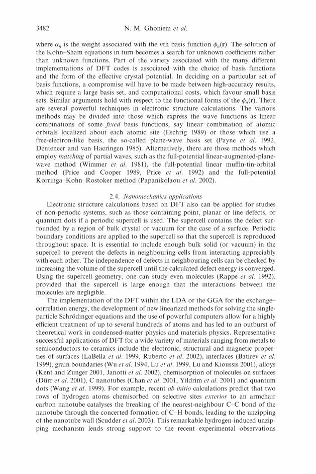
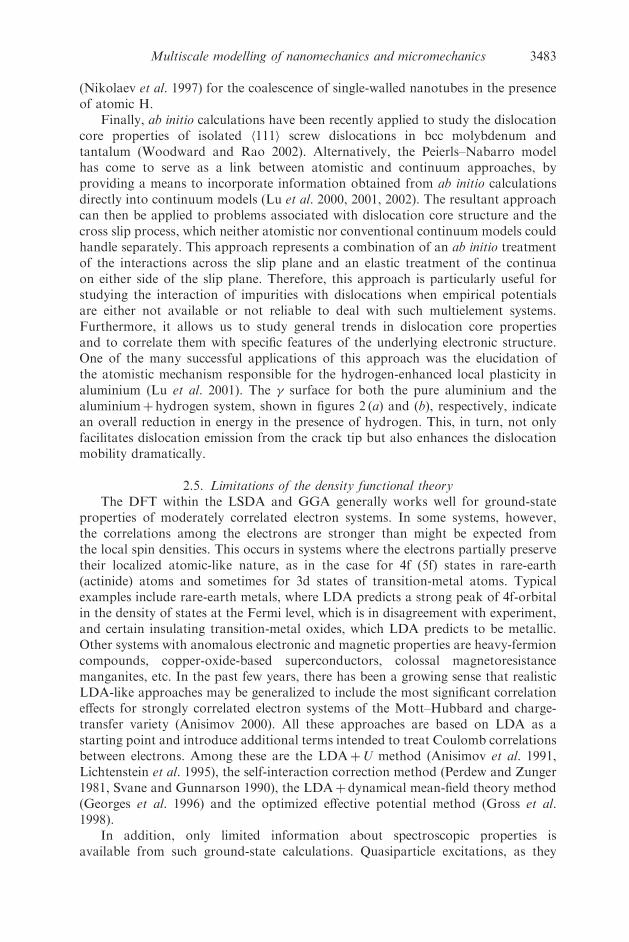
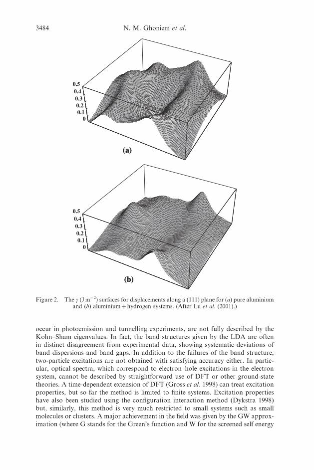
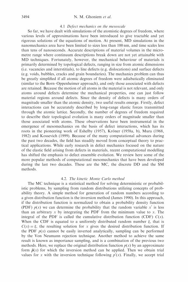
Finally, ab initio calculations have been recently applied to study the dislocationcore properties of isolated 111h i screw dislocations in bcc molybdenum andtantalum (Woodward and Rao 2002). Alternatively, the Peierls–Nabarro modelhas come to serve as a link between atomistic and continuum approaches, byproviding a means to incorporate information obtained from ab initio calculationsdirectly into continuum models (Lu et al. 2000, 2001, 2002). The resultant approachcan then be applied to problems associated with dislocation core structure and thecross slip process, which neither atomistic nor conventional continuum models couldhandle separately. This approach represents a combination of an ab initio treatmentof the interactions across the slip plane and an elastic treatment of the continuaon either side of the slip plane. Therefore, this approach is particularly useful forstudying the interaction of impurities with dislocations when empirical potentialsare either not available or not reliable to deal with such multielement systems.Furthermore, it allows us to study general trends in dislocation core propertiesand to correlate them with specific features of the underlying electronic structure.One of the many successful applications of this approach was the elucidation ofthe atomistic mechanism responsible for the hydrogen-enhanced local plasticity inaluminium (Lu et al. 2001). The � surface for both the pure aluminium and thealuminiumþ hydrogen system, shown in figures 2 (a) and (b), respectively, indicatean overall reduction in energy in the presence of hydrogen. This, in turn, not onlyfacilitates dislocation emission from the crack tip but also enhances the dislocationmobility dramatically.

2.5. Limitations of the density functional theoryThe DFT within the LSDA and GGA generally works well for ground-state

properties of moderately correlated electron systems. In some systems, however,the correlations among the electrons are stronger than might be expected fromthe local spin densities. This occurs in systems where the electrons partially preservetheir localized atomic-like nature, as in the case for 4f (5f) states in rare-earth(actinide) atoms and sometimes for 3d states of transition-metal atoms. Typicalexamples include rare-earth metals, where LDA predicts a strong peak of 4f-orbitalin the density of states at the Fermi level, which is in disagreement with experiment,and certain insulating transition-metal oxides, which LDA predicts to be metallic.Other systems with anomalous electronic and magnetic properties are heavy-fermioncompounds, copper-oxide-based superconductors, colossal magnetoresistancemanganites, etc. In the past few years, there has been a growing sense that realisticLDA-like approaches may be generalized to include the most significant correlationeffects for strongly correlated electron systems of the Mott–Hubbard and charge-transfer variety (Anisimov 2000). All these approaches are based on LDA as astarting point and introduce additional terms intended to treat Coulomb correlationsbetween electrons. Among these are the LDAþU method (Anisimov et al. 1991,Lichtenstein et al. 1995), the self-interaction correction method (Perdew and Zunger1981, Svane and Gunnarson 1990), the LDAþ dynamical mean-field theory method(Georges et al. 1996) and the optimized effective potential method (Gross et al.1998).

In addition, only limited information about spectroscopic properties isavailable from such ground-state calculations. Quasiparticle excitations, as they


occur in photoemission and tunnelling experiments, are not fully described by theKohn–Sham eigenvalues. In fact, the band structures given by the LDA are oftenin distinct disagreement from experimental data, showing systematic deviations ofband dispersions and band gaps. In addition to the failures of the band structure,two-particle excitations are not obtained with satisfying accuracy either. In partic-ular, optical spectra, which correspond to electron–hole excitations in the electronsystem, cannot be described by straightforward use of DFT or other ground-statetheories. A time-dependent extension of DFT (Gross et al. 1998) can treat excitationproperties, but so far the method is limited to finite systems. Excitation propertieshave also been studied using the configuration interaction method (Dykstra 1998)but, similarly, this method is very much restricted to small systems such as smallmolecules or clusters. A major achievement in the field was given by the GW approx-imation (where G stands for the Green’s function and W for the screened self energy


(a)

00.10.20.30.40.5

(a)

(b)

00.10.20.30.40.5

(b)

Figure 2. The g (Jm�2) surfaces for displacements along a (111) plane for (a) pure aluminiumand (b) aluminiumþ hydrogen systems. (After Lu et al. (2001).)

correction) (Hedin and Lundqvist 1969) for the self-energy, which allows for a veryaccurate evaluation of the self-energy on the basis of results from a preceding DFTcalculation. Highly accurate band structures for real materials have been obtained bythis method, including bulk semiconductors, insulators, metals, semiconductor sur-faces, atoms, defects and clusters, thus making the GWA a standard tool in predict-ing the electron quasiparticle spectrum of moderately correlated electron systems(Louie 1996).

2.6. Connections to interatomic potentialsThe direct use of DFT methods to perform full quantumMD simulations on real

materials is limited to a hundred or so atoms and a simulation time of a fewpicoseconds. Thus, the next step of coarse graining the problem is to remove theelectronic degrees of freedom by imagining the atoms to be held together by somesort of glue or interatomic potential, thereby allowing large-scale atomistic simula-tions for millions of atoms and a simulation time of nanoseconds. Such simulations,employing either the embedded-atom method (EAM) type (Daw and Baskes 1983,1984) or the Finnis–Sinclair (1984) type in metals, and the Stillinger–Weber (1985)type (Ackland and Vitek 1990) or the Tersoff (1986) type in covalent materials,have been extremely useful in investigating generic phenomena in simple systems.Empirical potentials involve the fitting of parameters to a predetermined experi-mental or ab initio database, which includes physical quantities such as the latticeconstant, the elastic constants, the vacancy formation energy and the surface energy.However, at the same time, they may not provide the desired physical accuracy formany real complex materials of interest. For example, reliable interatomic potentialsusually are not available for multielement materials and for systems containingsubstitutional or interstitial alloying impurities.

There is consequently growing need to develop more accurate interatomicpotentials, derived from QM, that can be applied to large-scale atomistic simulations.This is especially so for directionally bonded systems, such as transition metals, andfor chemically or structurally complex systems, such as intermetallics and alloys. Thetight-binding (TB) (Cohen et al. 1994, Mehl and Papaconstantopoulos 1996) and theself-consistent-charge density functional TB MD approach is becoming widespreadin the atomistic simulation community, because it allows one to evaluate both ionicand electronic properties (Frauenheim et al. 1998). The success of TB MD stands ona good balance between the accuracy of the physical representation of the atomicinteractions and the resulting computational cost. TB MD implements an empiricalparametrization of the bonding interactions based on the expansion of the electronicwave functions on a very simple basis set. Recently, novel analytic bond-orderpotentials have been derived for atomistic simulations by coarse graining the elec-tronic structure within the orthogonal two-centre TB representation (Pettifor 1989,Pettifor and Oleinik 1999, 2000). Quantum-based interatomic potentials for transi-tion metals that contain explicit angular-force contributions have been developedfrom first-principles, DFT-based generalized pseudopotential theory (Moriarty 1988,Moriarty and Widom 1997, Moriarty et al. 2002).

2.7. Linear scaling electronic structure methodsAwealth of efficient methods, the so-called order-N (O(N)) methods, have recently

been developed (Yang 1991, Li et al. 1993, Ordejon et al. 1993, Goedecker 1999) for


calculating the electronic properties of an extended system that require an amountof computation that scales linearly with the size N of the system. On the contrary,the widely used Carr–Parinello (1985) MD methods and various minimization tech-niques (Payne et al. 1992) are limited because the computational time required scalesas N3, where N can be defined to be the number of atoms or the volume of thesystem. Thus, these methods are an essential tool for the calculation of the electronicstructure of large systems containing many atoms. Most O(N) algorithms are builtaround the density matrix or its representation in terms of Wannier functions(Marzari and Vanderbilt 1997) and take advantage of its decay properties. To obtainlinear scaling, one has to cut off the exponentially decaying quantities when they aresmall enough. This introduces the concept of a localization region. Only inside thislocalization region is the quantity calculated; outside it is assumed to vanish. Forsimplicity the localization region is usually taken to be a sphere, even though theoptimal shape might be different.

O(N) methods have become as essential part of most large-scale atomisticsimulations based on either TB or semiempirical methods. The use of O(N) methodswithin DFT methods is not yet widespread. All the algorithms that would allow us totreat very large basis sets within DFT have certain shortcomings. An illustration ofthe wide range of areas where O(N) methods have made possible the study of systemsthat were too large to be studied with conventional methods include the 90� partialdislocation in silicon (Nunes et al. 1996), the surface reconstruction properties ofsilicon nanobars (Ismail-Beigi and Arias 1999), the molecular crash simulation of C60

fullerenes colliding with a diamond surface (Galli and Mauri 1994), the irradiation-mediated knockout of carbon atoms from carbon nanotubes (Ajayan et al. 1998) andthe geometric structure of large bimolecules (Lewis et al. 1997).

} 3. Large-scale atomistic simulations

The ab initio methods presented in } 2 are rigorous but limited by present-daycomputers to systems containing a few hundred atoms at most. Such methodsserve two important purposes. Firstly, they provide direct information on theresponse of materials to external environments (e.g. force and temperature).Secondly, they also generate a database of properties that can be used to constructeffective (empirical) interatomic potentials. To determine the properties of an ensem-ble of atoms larger than can be handled by computational QM, the description of theatomic interactions must be approximated. The MD method is developed to enablestudies of the properties of material volumes containing millions to billions of atomswith effective interatomic potentials. The basic idea is to eliminate all electronicdegrees of freedom and to assume that the electrons are glued to the nuclei. Thus,the interaction between two atoms is represented by a potential function that dependson the atomic configuration (i.e. relative displacement) and the local environment(i.e. electrons). Based on the electronic structure database, or alternatively usingexperimental measurements of specific properties, approximate effective potentialscan be constructed. According to classical Newtonian mechanics, the dynamicevolution of all atoms can be fully determined by numerical integration. In principle,once the positions and velocities of atoms in the finite ensemble within the simu-lation cell are known, all thermodynamic properties can be readily extracted.The implementation and practice of MD simulations are more involved than theconceptual description alluded to here. A successful simulation depends on three


major factors:

(i) the computational implementation of the MD method;(ii) the construction of accurate interatomic potentials; and(iii) the analysis of massive data resulting from computer simulations.

In the following, we briefly present key concepts in the numerical implementationof MD methods and then discuss salient aspects of the last two topics.

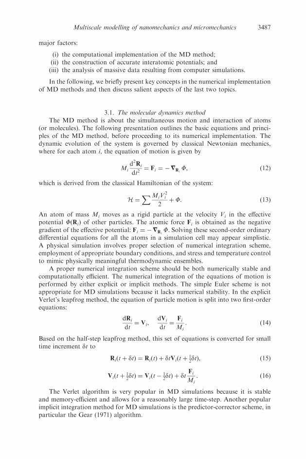
3.1. The molecular dynamics methodThe MD method is about the simultaneous motion and interaction of atoms

(or molecules). The following presentation outlines the basic equations and princi-ples of the MD method, before proceeding to its numerical implementation. Thedynamic evolution of the system is governed by classical Newtonian mechanics,where for each atom i, the equation of motion is given by

Mi

d2Ri

dt2¼ Fi ¼ �=Ri

F, ð12Þ

which is derived from the classical Hamiltonian of the system:

H ¼XMiV

2i

2þ F: ð13Þ

An atom of mass Mi moves as a rigid particle at the velocity Vi in the effectivepotential FðRiÞ of other particles. The atomic force Fi is obtained as the negativegradient of the effective potential: Fi ¼ �=Ri

F. Solving these second-order ordinarydifferential equations for all the atoms in a simulation cell may appear simplistic.A physical simulation involves proper selection of numerical integration scheme,employment of appropriate boundary conditions, and stress and temperature controlto mimic physically meaningful thermodynamic ensembles.

A proper numerical integration scheme should be both numerically stable andcomputationally efficient. The numerical integration of the equations of motion isperformed by either explicit or implicit methods. The simple Euler scheme is notappropriate for MD simulations because it lacks numerical stability. In the explicitVerlet’s leapfrog method, the equation of particle motion is split into two first-orderequations:

dRi

dt¼ Vi,

dVi

dt¼

Fi

Mi

: ð14Þ

Based on the half-step leapfrog method, this set of equations is converted for smalltime increment dt to

Riðtþ dtÞ ¼ RiðtÞ þ dtViðtþ12dtÞ, ð15Þ

Viðtþ12dtÞ ¼ Viðt�

12dtÞ þ dt

Fi

Mi

: ð16Þ

The Verlet algorithm is very popular in MD simulations because it is stableand memory-efficient and allows for a reasonably large time-step. Another popularimplicit integration method for MD simulations is the predictor-corrector scheme, inparticular the Gear (1971) algorithm.


Similar to the numerical integration scheme, proper use of boundary conditionsis crucial to obtaining a physically meaningful MD simulation. The boundary of asimulation cell is usually within close proximity to each simulated atom, because oflimited computational power. Simulations for 109 atoms represent the upper limit ofcomputation today with simple interatomic potentials (for examples see Lennard-Jones (1924)). Total simulation times are typically less than 10 ns as a result of shortintegration time steps in the femtosecond range. The boundary of a simulation cellmay not be a real physical interface, rather it is merely the interface of the simulationcell and its surroundings. Various boundary conditions are used in mechanics simu-lations. Since dislocations dominate the linking of nanomechanics and micromecha-nics, the following presentation focuses on those boundary conditions relevant to thelong-range strain fields of dislocations. These include the rigid boundary condition(Kuramoto et al. 2000), the periodic boundary condition (Kido et al. 2000), thedirect linking of atomistic and continuum regions (Oritz and Phillips 1999), andthe flexible (Green’s function) boundary condition (Sinclair 1971, Hoagland 1976,Woo and Puls 1976, Rao et al. 1998).

The rigid boundary condition is probably the simplest. According to this condi-tion, boundary atoms are fixed during MD simulations. For simple dislocationconfigurations, the initial strain field, say of an infinitely long straight dislocation,is imposed on all atoms in the simulation cell. During subsequent simulations,boundary atoms are not allowed to relax. This rigidity of the boundary conditionnaturally leads to inaccuracy in the simulation results. The inaccuracy also exists inthe application of the periodic boundary condition. Here, the simulation cell isrepeated periodically to fill the entire space. When one dislocation is included inthe simulation cell, an infinite number of its images are included in the entire spacebecause of the infinite repetition of the simulation cell. Modifications have beenmade to include dipoles in a simulation cell, and to subtract the image effects.However, it is difficult to extend such modifications to general dislocation config-urations, which are more complex.

In contrast with the two approximate boundary conditions, the direct linkingand flexible boundary conditions can be rigorous. The direct linking of atomistic andcontinuum region (Qrtiz and Phillips 1999) aims at seamless bridging of two differentscales. This idea has been extended to include direct linking of atomistic and electro-nic structure regions (Abraham et al. 1987). Once numerically robust and efficient,the direct linking scheme should be the most reliable and desirable boundary con-dition. At present, the other rigorous scheme, namely the flexible boundary condi-tion, is more commonly used in dislocation simulations. This scheme has gonethrough the implementations in two and three dimensions. In the 1970s, the two-dimensional version of this boundary condition was implemented (Sinclair 1971,Hoagland et al. 1976, Woo and Puls 1976), allowing the simulation of a singlestraight dislocation. In these simulations, periodic boundary conditions are appliedalong the dislocation line. On the plane normal to the dislocation line, the simulationcell is divided into three regions. The innermost region is the MD region, in whichatoms follow Newtonian dynamics according to the MD method outlined earlier.The intermediate region is the flexible region (or Green’s function region), in whichthe force on each atom is calculated and then used to generate displacements ofall atoms in the simulation cell according to the Green’s function of displacement.Since a periodic boundary condition is applied along the dislocation line, line forcesare calculated in the flexible region, making the displacement two dimensional. The


outermost region contains atoms that serve as background for force calculations inthe flexible region. As a result of renewed interest in DD, flexible boundary condi-tions have been extended to three dimensions and are often referred to as the Green’sfunction boundary conditions (Rao et al. 1998). Flexible or Green’s function bound-ary conditions have clear advantages in allowing for full relaxation of one or a fewdislocations in a simulation cell, without suffering from the artefacts of image dis-locations. However, Green’s function calculations are time-consuming limitingapplications of the Green’s function boundary condition. Recently, a tabulationand interpolation scheme (Golubov et al. 2001) has been developed, improving thecomputational efficiency by two orders of magnitude and yet maintaining the accu-racy of linear elasticity. With this improvement, the Green’s function boundaryconditions work well for static simulations of dislocations. However, they are notapplicable to truly dynamic simulations. During dislocation motion, elastic wavesare emitted and, when they interact with the simulation cell boundaries or borders,they are reflected and can lead to interference or even resonance in the simulationcell. Approximate approaches (Ohsawa and Kuramoto 1999, Cai et al. 2000) havebeen proposed to damp the waves at the boundary, but a fully satisfactory solution isstill not available.

In addition to the numerical integration and boundary condition issues, success-ful MD simulations rely on the proper control of thermodynamic variables: stressand temperature. When the internal stress, as derived from interatomic interactions,is not balanced by the external stress, the simulation cell deforms accordingly. At lowstress levels, this response is consistent with linear elasticity. Under general stressconditions, the formulation of Parrinello and Rahman (1981) provides a mechanismto track the deformation. In this formulation, the three vectors describing theshape of simulation cell are equated to position vectors of three imaginary atoms.The driving force of the imaginary atoms is the imbalance of internal and externalstresses, and the movements of those atoms are governed by Newton’s equations ofmotion. This formulation works well when an equilibrated stress state is sought.However, large fluctuations in the deformation are unavoidable according to theParrinello–Rahman method; the lattice constant may fluctuate by about 0.5%around its equilibrium value. This large fluctuation may introduce artefacts in thesimulation of kinetic process, and caution should be exercised. The other thermo-dynamic variable, temperature, is controlled through the kinetic energy or velocitiesof all atoms. Using frictional forces to add or subtract heat, the Nose (1984)–Hoover(1985) method provides a mechanism of controlling the temperature of a simulationcell. When the temperature is uniform in space and constant in time, little difficultyexists. When the temperature changes, however, the strength of the frictional forcedictates the transition time. A fast transition is usually necessary because of the shorttime reachable in MD simulations. However, such a transition is generally too fastcompared with realistic processes. This transition problem exists in other tempera-ture control mechanisms, such as velocity scaling or introduction of random forces.

3.2. Interatomic potentialsA proper MD method is a necessary condition for physically meaningful simu-

lations. However, the method says nothing about how simulated atoms interactwith each other. The latter aspect is solely determined by prescribed interatomicpotentials and is more crucial in obtaining physically meaningful results. In general,there is a compromise between the potential rigorousness and the computational


efficiency. For high computational efficiency, pair potentials, such as the Lennard-Jones (1924) and the Morse (1929) potentials are used. With the increasing demandon accuracy and available computational power, many-body potentials such as theFinnis–Sinclair (1984) potential and the EAM (Daw and Baskes 1983, 1984) havebeen commonly used. In the same category are effective-medium and glue models(Ercolessi et al. 1986). Angle-dependent potentials, which are also many-body,include the well-known Stillinger–Weber (1985) potential and the Tersoff (1986)potential. Potentials that have a QM basis, such as the generalized pseudopotential(Moriarty 1988, 1994), the bond order potential (Pettifor 1989) and the inversionmethod (Chen 1990, Zhang et al. 1997) have also been used for greater accuracy.

In general, interatomic potentials are empirical or semiempirical and therebyhave fitting parameters. Simpler potentials, like the Lennard-Jones potential, havevery few fitting parameters, which can be easily determined from crystal properties.On the other hand, these potentials suffer from non-transferability. Since thesepotentials are fitted to only a few perfect crystal properties, their applicability instudying defects is by default questionable. The more sophisticated potentials, likethe EAM, particularly the force matching approach (Ercolessi and Adams 1994), useseveral or many defect properties to determine the EAM functions, in either analy-tical or tabular form. Materials properties, of either the perfect crystal or the defec-tive structures, are obtained from ab initio calculations and reliable experiments. It isworth pointing out that these interatomic potentials apply for specific classes ofmaterials. Strictly speaking, pair potentials are applicable to simulations of rare-gas behaviour. However, applications to simple metal systems can also providequalitative guidance. The EAM type of potential has proven to be a good choicefor simple metals. Applications to metals such as aluminium, copper, silver and iron(except its magnetic properties) have been very successful. The radial function formof the EAM is computationally advantageous. However, this advantage is accom-panied by the inability to describe covalent systems, in which angular dependencedominates. In studying silicon, diamond, carbon and other covalent systems, angulardependent potentials, particularly the Stillinger–Weber (1985) potential, the Tersoff(1986) potential, and the bond-order potential (Pettifor 1989) are among the leadingcandidates. A modification of the EAM has been proposed to include the angulardependence by Baskes (1987), and applied to SiC by Huang et al. (1995); the mod-ification by Pasianot et al. (1991) is similar.

3.3. Applications of atomistic simulations in mechanicsThis section focuses on the applications of MD simulations to mechanics

problems at the nanoscale. Furthermore, the presentation is focused on nano-mechanics of point defects, dislocations and interfaces (free surfaces and grainboundaries) under applied stress. Mechanics of nanotubes have also receivedmuch attention (Dumitrica et al. 2003) but will not be treated here.

We start with point defects. Under stress, the normal diffusion process governedby point defect motion is polarized by the action of the stress field. The diffusionprocess of a point defect has been investigated by a combination of molecular statics(MS) and MD simulations. Diffusion anisotropy, which is intrinsic in low-symmetrycrystals, can be enhanced by the action of stress (Woo et al. 2002). The stress effecton a point defect, in particular its formation and migration energies, is crucialto the analysis of kinetic processes, but this is usually not a first-order effect innanomechanics.


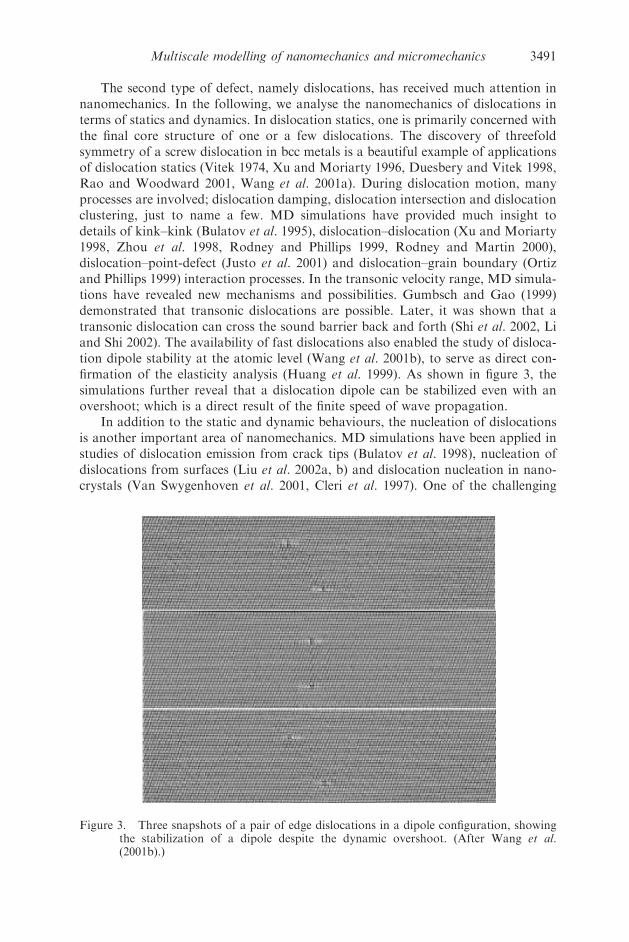
The second type of defect, namely dislocations, has received much attention innanomechanics. In the following, we analyse the nanomechanics of dislocations interms of statics and dynamics. In dislocation statics, one is primarily concerned withthe final core structure of one or a few dislocations. The discovery of threefoldsymmetry of a screw dislocation in bcc metals is a beautiful example of applicationsof dislocation statics (Vitek 1974, Xu and Moriarty 1996, Duesbery and Vitek 1998,Rao and Woodward 2001, Wang et al. 2001a). During dislocation motion, manyprocesses are involved; dislocation damping, dislocation intersection and dislocationclustering, just to name a few. MD simulations have provided much insight todetails of kink–kink (Bulatov et al. 1995), dislocation–dislocation (Xu and Moriarty1998, Zhou et al. 1998, Rodney and Phillips 1999, Rodney and Martin 2000),dislocation–point-defect (Justo et al. 2001) and dislocation–grain boundary (Ortizand Phillips 1999) interaction processes. In the transonic velocity range, MD simula-tions have revealed new mechanisms and possibilities. Gumbsch and Gao (1999)demonstrated that transonic dislocations are possible. Later, it was shown that atransonic dislocation can cross the sound barrier back and forth (Shi et al. 2002, Liand Shi 2002). The availability of fast dislocations also enabled the study of disloca-tion dipole stability at the atomic level (Wang et al. 2001b), to serve as direct con-firmation of the elasticity analysis (Huang et al. 1999). As shown in figure 3, thesimulations further reveal that a dislocation dipole can be stabilized even with anovershoot; which is a direct result of the finite speed of wave propagation.

In addition to the static and dynamic behaviours, the nucleation of dislocationsis another important area of nanomechanics. MD simulations have been applied instudies of dislocation emission from crack tips (Bulatov et al. 1998), nucleation ofdislocations from surfaces (Liu et al. 2002a, b) and dislocation nucleation in nano-crystals (Van Swygenhoven et al. 2001, Cleri et al. 1997). One of the challenging


Figure 3. Three snapshots of a pair of edge dislocations in a dipole configuration, showingthe stabilization of a dipole despite the dynamic overshoot. (After Wang et al.(2001b).)

problems that remain is treating the interaction of boundaries with elastic wavesemitted by a moving dislocation. It is usually necessary to separate this interactionfrom the true dynamics of a moving dislocation. Several recent studies haveattempted to damp out boundary effects (Ohsawa and Kuramoto 1999, Cai et al.2000, Wang et al. 2001b), but the problem is still not satisfactorily solved.

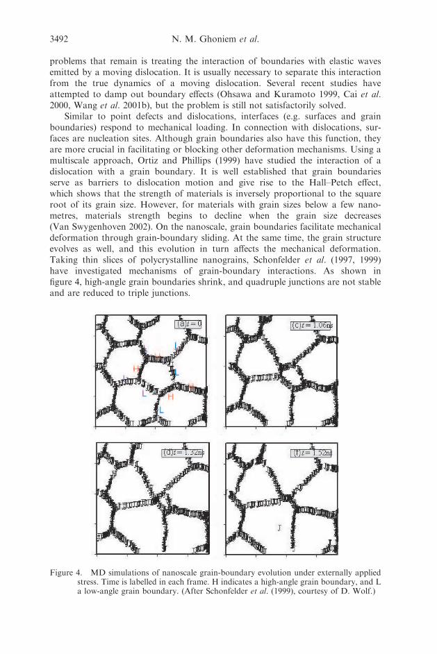
Similar to point defects and dislocations, interfaces (e.g. surfaces and grainboundaries) respond to mechanical loading. In connection with dislocations, sur-faces are nucleation sites. Although grain boundaries also have this function, theyare more crucial in facilitating or blocking other deformation mechanisms. Using amultiscale approach, Ortiz and Phillips (1999) have studied the interaction of adislocation with a grain boundary. It is well established that grain boundariesserve as barriers to dislocation motion and give rise to the Hall–Petch effect,which shows that the strength of materials is inversely proportional to the squareroot of its grain size. However, for materials with grain sizes below a few nano-metres, materials strength begins to decline when the grain size decreases(Van Swygenhoven 2002). On the nanoscale, grain boundaries facilitate mechanicaldeformation through grain-boundary sliding. At the same time, the grain structureevolves as well, and this evolution in turn affects the mechanical deformation.Taking thin slices of polycrystalline nanograins, Schonfelder et al. (1997, 1999)have investigated mechanisms of grain-boundary interactions. As shown infigure 4, high-angle grain boundaries shrink, and quadruple junctions are not stableand are reduced to triple junctions.


Figure 4. MD simulations of nanoscale grain-boundary evolution under externally appliedstress. Time is labelled in each frame. H indicates a high-angle grain boundary, and La low-angle grain boundary. (After Schonfelder et al. (1999), courtesy of D. Wolf.)

The presentation in this section has so far focused on physical aspect of nano-mechanics. This physical understanding relies on identification and analysis of pointdefects, dislocations and interfaces. Among the three types of defects, dislocationsare probably the most difficult to characterize or identify. The identification isstraightforward if the dislocation configuration is simple. One may rely on construct-ing the Burgers circuit, using disregistry functions (such as the centro-symmetryparameter), or tracking the atomic level stress or energy (Hamilton 1997,Hamilton et al. 1999, Chang et al. 2001). When complex dislocation configurationsare involved, unambiguous identification of dislocation cores may require a combi-nation of several of the methods discussed above. There is still not a universalcharacterization method that fits all purposes.

Before closing this section, let us examine the type of information that can bepassed on to larger length scales. Here, we consider three types of defects: pointdefects, dislocations, and interfaces (particularly grain boundaries). Information ondefect energetics and diffusion tensors obtained by MD or MS simulationsprovide parameters to rate equations and MC methods describing microstructureevolutions. Dislocation energetics (e.g. kink-pair formation energy and dislocationcore energy), Peierls stress and dislocation mobility are used as input parameters indislocation dynamics simulations at the mesoscopic level (Bulatov et al. 1998).Finally, dislocation nucleation conditions and interaction mechanisms with otherdefects (dislocations or grain boundaries or other interfaces) from MD simulationsare critical to DD simulations.

} 4. Mesomechanics and the role of defects

Studies of the mechanical behaviour of materials on a length scale larger thanwhat can be handled by direct atomistic simulations and smaller than what is poss-ible with continuum mechanics represent particular difficulties. Two complementaryapproaches have been advanced to model the mechanical behaviour in this meso-scopic length scale. The first approach, that of DD, was initially motivated by theneed to understand the origins of heterogeneous plasticity and pattern formation. Anearly variant of this approach (the cellular automata) was first developed byLepinoux and Kubin (1987), and that was followed by the proposal of DD(Ghoniem and Amodeo 1988a, b, Amodeo and Ghoniem 1990a, b). In these earlyefforts, dislocation ensembles were modelled as infinitely long and straight inan isotropic infinite elastic medium. The method was further expanded by a numberof researchers (Guluoglu et al. 1989, Lubarda and Needleman 1993, Barts andCarlsson 1995, 1998, Wang and LeSar 1995), with applications demonstratingsimplified features of deformation microstructure.

The second approach to mechanical models on the mesoscale has been based onSM methods (Walgraef and Aifantis 1985, Gregor and Kratochvil 1990, Kratochviland Saxlova 1992, Saxlova et al. 1997, Hahner et al. 1998, Zaiser et al. 1998,El-Azab 2000, Thomson et al. 2002). In these developments, evolution equationsfor statistical averages (and possibly for higher moments) are to be solved for acomplete description of the deformation problem. The main challenge in this regardis that, unlike the situation encountered in the development of the kinetic theoryof gases, the topology of interacting dislocations within the system must be included(El-Azab 2000). In the following, we review the main theoretical and computationaladvances in mesomechanics.


4.1 Defect mechanics on the mesoscaleSo far, we have dealt with simulations of the atomistic degrees of freedom, where

various levels of approximations have been introduced to give tractable and yetrigorous solutions of the equations of motion. At present, MD simulations in thenanomechanics area have been limited to sizes less than 100 nm, and time scales lessthan tens of nanoseconds. Accurate descriptions of material volumes in the micro-metre range where continuum descriptions break down are not yet attainable withMD techniques. Fortunately, however, the mechanical behaviour of materials isprimarily determined by topological defects, ranging in size from atomic dimensions(i.e. vacancies and interstitials), to line defects (e.g. dislocations) and surface defects(e.g. voids, bubbles, cracks and grain boundaries). The mechanics problem can thusbe greatly simplified if all atomic degrees of freedom were adiabatically eliminated(similar to the Born–Oppenheimer approach), and only those associated with defectsare retained. Because the motion of all atoms in the material is not relevant, and onlyatoms around defects determine the mechanical properties, one can just followmaterial regions around defects. Since the density of defects is many orders ofmagnitude smaller than the atomic density, two useful results emerge. Firstly, defectinteractions can be accurately described by long-range elastic forces transmittedthrough the atomic lattice. Secondly, the number of degrees of freedom requiredto describe their topological evolution is many orders of magnitude smaller thanthose associated with atoms. These observations have been instrumental in theemergence of mesomechanics on the basis of defect interactions, which has itsroots in the pioneering work of Eshelby (1957), Kroner (1958a, b), Mura (1968,1982) and Kossevich (1999). Because of the many computational advances duringthe past two decades, the field has steadily moved from conceptual theory to prac-tical applications. While early research in defect mechanics focused on the natureof the elastic field arising from defects in materials, recent computational modellinghas shifted the emphasis to defect ensemble evolution. We review here some of themore popular methods of computational mesomechanics that have been developedduring the last two decades. These are the MC, the discrete DD and the SMmethods.

4.2. The kinetic Monte Carlo methodThe MC technique is a statistical method for solving deterministic or probabil-

istic problems, by sampling from random distributions utilizing concepts of prob-ability theory. A simple method for generation of random numbers according toa given distribution function is the inversion method (James 1990). In this approach,if the distribution function is normalized to obtain a probability density function(PDF) pðxÞ we can determine the probability that the random variable x0 is lessthan an arbitrary x by integrating the PDF from the minimum value to x. Theintegral of the PDF is called the cumulative distribution function (CDF) CðxÞ.When the CDF is equated to a uniformly distributed random number , that isCðxÞ ¼ , the resulting solution for x gives the desired distribution function. Ifthe PDF pðxÞ cannot be easily inverted analytically, sampling can be performedby the Von Neumann rejection technique. Another method to achieve the sameresult is known as importance sampling, and is a combination of the previous twomethods. Here, we replace the original distribution function pðxÞ by an approximateform ~ppðxÞ for which the inversion method can be applied. Then we obtain trialvalues for x with the inversion technique following p0ðxÞ. Finally, we accept trial


values with the probability proportional to the weight w, given by w ¼ pðxÞ= ~ppðxÞ.The rejection technique has been shown to be a special case of importance sampling,where p0ðxÞ is a constant (James 1980).

When the configurational space is discrete, and all rates at which they occurcan be determined, we can choose and execute a single change to the system fromthe list of all possible changes at each MC step. This is the general idea of the kineticMonte Carlo (KMC) method (Doran 1970, Beeler 1982, Heinisch 1995). The mainadvantage of this approach is that it can take into account simultaneous differentmicroscopic mechanisms and can cover very different time scales.

First, we tabulate the rates at which each event will occur anywhere in thesystem: ri. The probability of event occurrence is defined as the rate at which theevent takes place relative to the sum of all possible event rates. Once an event isselected, the system is changed, and the list of events that can occur at the next stepis updated. Hence, one event denoted by m is randomly chosen from all of theM events that can possibly occur, as follows:

Xm�1

i¼0

ri

�XMi¼0

ri < <Xmi¼0

ri

�XMi¼0

ri, ð17Þ

where ri is the rate at which event i occurs (r0 ¼ 0) and is a random numberuniformly distributed in the range [2 ð0, 1Þ].

After a particular event is selected, the table of all possible events is updated(Battaile and Srolovitz 1997). In the Metropolis et al. (1953) scheme, a fixed timeincrement is chosen such that at most one event occurs during a time step. However,this approach is inefficient since, in many time steps, no events will happen. Analternative technique, known as the n-fold way algorithm and introduced by Bortzet al. (1975), ensures that one event occurs somewhere in the system. Thus, the timeincrement itself, dt, corresponding to each step is variable, because it depends on thecorresponding event probability, as

�t ¼ � ln ðÞ

�XMi¼1

ri: ð18Þ

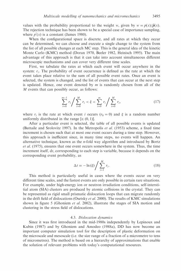
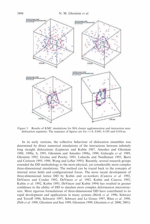
This method is particularly useful in cases where the events occur on verydifferent time scales, and the fastest events are only possible in certain rare situations.For example, under high-energy ion or neutron irradiation conditions, self-intersti-tial atom (SIA) clusters are produced by atomic collisions in the crystal. They canbe represented as rigid small prismatic dislocation loops that can migrate randomlyin the drift field of dislocations (Osetsky et al. 2000). The results of KMC simulationsshown in figure 5 (Ghoniem et al. 2002), illustrate the stages of SIA motion andclustering in the stress field of dislocations.

4.3. Dislocation dynamicsSince it was first introduced in the mid-1980s independently by Lepinoux and

Kubin (1987) and by Ghoniem and Amodeo (1988a), DD has now become animportant computer simulation tool for the description of plastic deformation onthe microscale and mesoscale (i.e. the size range of a fraction of a micrometre to tensof micrometres). The method is based on a hierarchy of approximations that enablethe solution of relevant problems with today’s computational resources.


In its early versions, the collective behaviour of dislocation ensembles wasdetermined by direct numerical simulations of the interactions between infinitelylong straight dislocations (Lepinoux and Kubin 1987, Amodeo and Ghoniem1988, 1990a, b, 1991, Ghoniem and Amodeo 1988a, 1990, Guluoglu et al. 1989,Ghoniem 1992, Groma and Pawley 1993, Lubarda and Needleman 1993, Bartsand Carlsson 1995, 1998, Wang and LeSar 1995). Recently, several research groupsextended the DD methodology to the more physical, yet considerably more complexthree-dimensional simulations. The method can be traced back to the concepts ofinternal stress fields and configurational forces. The more recent development ofthree-dimensional lattice DD by Kubin and co-workers (Canova et al. 1992,DeVincre and Condat 1992, DeVincre et al. 1992, Kubin and Canova 1992,Kubin et al. 1992, Kubin 1993, DeVincre and Kubin 1994) has resulted in greaterconfidence in the ability of DD to simulate more complex deformation microstruc-ture. More rigorous formulations of three-dimensional DD have contributed to itsrapid development and applications in many systems (Hirth et al. 1996, Schwarzand Tersoff 1996, Schwartz 1997, Schwarz and Le Goues 1997, Rhee et al. 1998,Zbib et al. 1998, Ghoniem and Sun 1999, Ghoniem 1999, Ghoniem et al. 2000, 2001).


Figure 5. Results of KMC simulations for SIA cluster agglomeration and interaction neardislocation segments. The sequence of figures are for t¼ 0, 0.043, 0.189 and 0.416 ns.

When the Green’s functions are known, the elastic field of a dislocation loop canbe constructed by a surface integration. The starting point in this calculation is thedisplacement field in a crystal containing a dislocation loop, which can be expressedas (Volterra 1907, Mura 1968)

uiðxÞ ¼ �

ðS

Cjlmnbmo

o x0lGijðx, x

0Þnn dSðx

0Þ, ð19Þ

where Cjlmn is the elastic constants tensor, Gijðx,x0Þ are the Green’s functions at x due

to a point force applied at x0, S is the surface capping the loop, nn is a unit normal toS and bm is the Burgers vector. The elastic distortion tensor ui, j can be obtained fromequation (19) by differentiation. The symmetric part of ui, j (elastic strain tensor) isthen used in the stress–strain relationship to find the stress tensor at a field point x,caused by the dislocation loop.

In an elastically isotropic and infinite medium, a more efficient form of equation(19) can be expressed as a line integral performed over the closed dislocation loop(deWit 1960):

ui ¼ �bi4p

þC

Akdlk þ1

8p

þC

�ikibiR, pp þ1

1� �kmnbnR,mi

� �dlk, ð20Þ

where � and are the shear modulus and Poisson’s ratio respectively, b is theBurgers vector with the Cartesian components bi, and the vector potentialAkðRÞ ¼ �ijkXisj=RðRþ R � sÞ satisfies the differential equation �pikAk, pðRÞ ¼ XiR

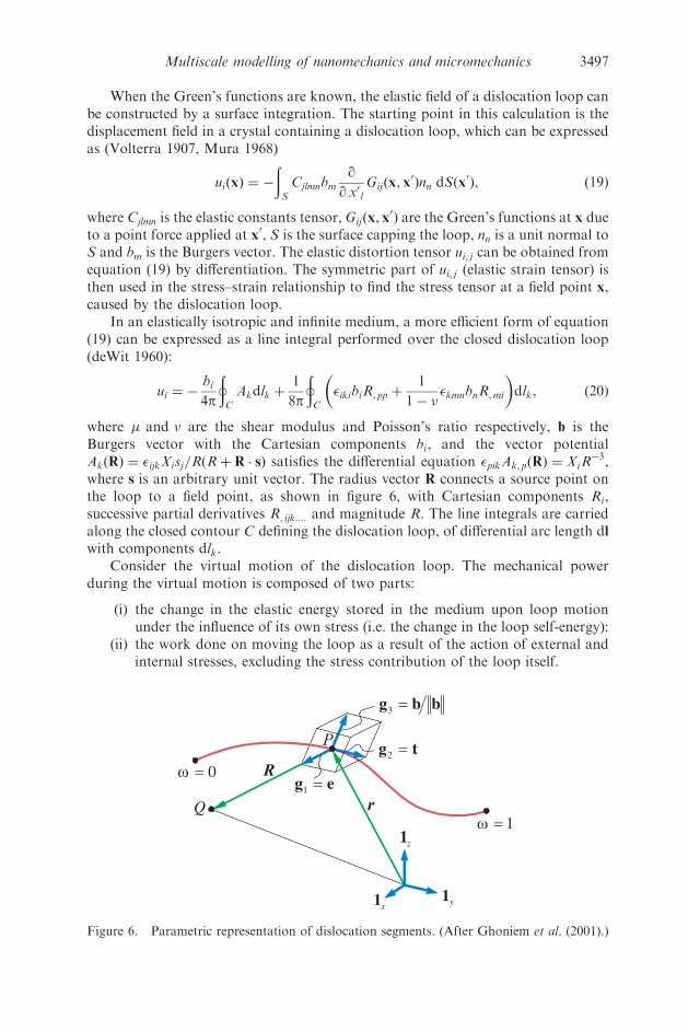
�3,where s is an arbitrary unit vector. The radius vector R connects a source point onthe loop to a field point, as shown in figure 6, with Cartesian components Ri,successive partial derivatives R, ijk...: and magnitude R. The line integrals are carriedalong the closed contour C defining the dislocation loop, of differential arc length dlwith components dlk.

Consider the virtual motion of the dislocation loop. The mechanical powerduring the virtual motion is composed of two parts:

(i) the change in the elastic energy stored in the medium upon loop motionunder the influence of its own stress (i.e. the change in the loop self-energy):

(ii) the work done on moving the loop as a result of the action of external andinternal stresses, excluding the stress contribution of the loop itself.


x1 y1

1

0

1

eg1

tg2

bbg =3

Q

Figure 6. Parametric representation of dislocation segments. (After Ghoniem et al. (2001).)

These two components constitute the Peach–Koehler (1950) work . The mainidea of DD is to derive approximate equations of motion from the principle ofvirtual power dissipation of the second law of thermodynamics (Ghoniem et al.2001), by finding virtual Peach–Kohler forces that would result in the simultaneousdisplacement of all dislocation loops in the crystal. A major simplification is that thismany-body problem is reduced to the single-loop problem. In this simplification,instead of moving all the loops simultaneously, they are moved sequentially, withthe motion of each one against the collective field of all other loops. The approachis reminiscent of the single-electron simplification of the many-electron problemin QM.

In finite systems, Green’s functions are not invariant under x ! x0 transforma-

tions, and they become functions of both source and field points (i.e. not functions ofthe radius vector alone any more). This does not allow the reduction of the surfaceintegral of equation (20) to a simpler line integral by application of the Stokestheorem. In addition, closed-form solutions for Green’s functions and their spatialderivatives are available only for elastically isotropic materials. Therefore, rigorousthree-dimensional DD in finite anisotropic systems (e.g. thin films and quantumdots) are very demanding and have not yet been implemented.

If the material is assumed to be elastically isotropic and infinite, a great reductionin the level of required computations ensues. Firstly, surface integrals can bereplaced by line integrals along the dislocation. Secondly, Green’s functions andtheir derivatives have analytical solutions. Thus, the starting point in most DDsimulations so far is a description of the elastic field of dislocation loops of arbitraryshapes by line integrals of the form proposed by deWit (1960) :

�ij ¼�

4p

þC

1

2R,mpp �jmndli þ �imndlj

� �þ

1

1� �kmn R, ijm � �ijR, ppm

� �dlk

� �, ð21Þ

where � and are the shear modulus and Poisson’s ratio respectively. The lineintegral is discretized, and the stress field of dislocation ensembles is obtained by asummation process over line segments.

Recently, Ghoniem and Sun (1999) and Ghoniem et al. (2001) have shown that,if dislocation loops are discretized into curved parametric segments, one can obtainthe field by numerical integration over the scalar parameter that represents thesegment. One of these segments is described by a parameter ! that varies, forexample, from 0 to 1 at end nodes of the segment. The segment is fully determinedas an affine mapping on the scalar interval 2 ½0, 1�, if we introduce the tangent vectorT, the unit tangent vector t and the unit radius vector e, as follows: T ¼ dl=d!,t ¼ T=jTj, e ¼ R=R. Let the Cartesian orthonormal basis set be denoted by1 � f1x, 1y, 1zg, I ¼ 1� 1 as the second-order unit tensor, and � denotes the tensorproduct. Now define the three vectors ðg1 ¼ e, g2 ¼ t, g3 ¼ b=jbjÞ as a covariantbasis set for the curvilinear segment, and their contravariant reciprocals asgi� gj ¼ �ij, where �

ij is the mixed Kronecker delta and V ¼ ðg1 � g2Þ � g3 the volume

spanned by the vector basis, as shown in figure 6.The differential stress field is given by

dr

d!¼

�V jTj

4pð1� ÞR2g1� g1 þ g1 � g

1� �

þ ð1� Þ g2 � g2 þ g2 � g2

� �� 3g1 � g1 þ I� ��

:

ð22Þ


Once the parametric curve for the dislocation segment is mapped on to thescalar interval {! 2 ½0, 1�}, the stress field everywhere is obtained as a fast numericalquadrature sum (Ghoniem and Sun 1999). The Peach–Kohler (1950) force exertedon any other dislocation segment can be obtained from the total stress field (externaland internal) at the segment as

FPK ¼ �b� t: ð23Þ

The total self-energy of the dislocation loop is determined by double line inte-grals. However, Gavazza (1976) have shown that the first variation in the self-energyof the loop can be written as a single line integral, and that the majority of thecontribution is governed by the local line curvature. Based on these methodsfor evaluations of the interaction and self-forces, the weak variational form of thegoverning equation of motion of a single dislocation loop was developed byGhoniem et al. (2000): ð

�

Ftk � B�kV�

� �drk dsj j ¼ 0: ð24Þ

Here, Ftk are the components of the resultant force, consisting of the Peach–Koehler

force FPK (generated by the sum of the external and internal stress fields), the self-force Fs and the osmotic force FO (in case climb is also considered (Ghoniem et al.2000). The resistivity matrix (inverse mobility) is B�k, V� are the velocity vectorcomponents, and the line integral is carried along the arc length of the dislocationds. To simplify the problem, let us define the following dimensionless parameters:

r�¼

r

a, f

�¼

F

�a, t� ¼

�t

B:

Here, a is lattice constant, � the shear modulus and t is time. Hence equation (24)can be rewritten in dimensionless matrix form asð

G�

d r�T � f��dr�

dt�

� �ds�� ¼ 0: ð25Þ

Here, f� ¼ ½f �1 , f�2 , f

�3 �

T, and r�¼ ½r�1, r

�2, r

�3�T, which are all dependent on the dimen-

sionless time t�. Following Ghoniem et al. (2000), a closed dislocation loop canbe divided into Ns segments. In each segment j, we can choose a set of generalizedcoordinates qm at the two ends, thus allowing parametrization of the form:

r�¼ CQ: ð26Þ

Here, C ¼ ½C1ð!Þ,C2ð!Þ, . . . ,Cmð!Þ�, Cið!Þ, ði ¼ 1, 2, . . . ,mÞ are shape functionsdependent on the parameter (04!4 1), and Q ¼ ½q1, q2, . . . , qm�

T, where qi are aset of generalized coordinates. Substituting equation (26) into equation (25) weobtain XNs

j¼1

ðGj

�QT� C

Tf�� C

TCdQ

dt�

� �dsj j ¼ 0 ð27Þ

Let

f j ¼

ðGj

CTf� dsj j, kj ¼

ðGj

CTC dsj j:


Following a similar procedure to the finite-element method, we assemble the equa-tion of motion for all contiguous segments in global matrices and vectors as

F ¼XNs

j¼1

f j , K ¼XNs

j¼1

kj;

then, from equation (27), we obtain

KdQ

dt�¼ F: ð28Þ

The solution of the set of ordinary differential equations (28) describes themotion of an ensemble of dislocation loops as an evolutionary dynamic system.However, additional protocols or algorithms are used to treat

(i) strong dislocation interactions (e.g. junctions or tight dipoles),(ii) dislocation generation and annihilation and(iii) adaptive meshing as dictated by large curvature variations (Ghoniem et al.

2000).

In the parametric method (Kukta and Freund 1998, Ghoniem 1999, Ghoniemet al. 2000, 2001) presented above, the dislocation loop can be geometrically repre-sented as a continuous (to second derivative) composite space curve. This has twoadvantages: firstly, there is no abrupt variation or singularities associated with theself-force at the joining nodes in between segments; secondly, very drastic variationsin dislocation curvature can be easily handled without excessive remeshing. Otherapproximation methods have been developed by a number of groups. Theseapproaches differ mainly in the representation of dislocation loop geometry, themanner by which the elastic field and self-energies are calculated, and some addi-tional details related to how boundary and interface conditions are handled. Thesuitability of each method is determined by the required level of accuracy andresolution in a given application.

Generally, coarse resolution is obtained by the lattice method, developed byKubin et al. (1992) and Moulin et al. (1997), where straight dislocation segments(either pure screw or edge in the earliest versions, or of a mixed character in morerecent versions) are allowed to jump on specific lattice sites and orientations. Straightdislocation segments of mixed character in the the force method, developed by Hirthet al. (1996) and Zbib et al. (1998) are moved in a rigid-body fashion along thenormal to their midpoints, but they are not tied to an underlying spatial lattice orgrid. The advantage of this method is that the explicit information on the elastic fieldis not necessary, since closed-form solutions for the interaction forces are directlyused. The differential stress method developed by Schwarz and Tersoff (1996) andSchwarz (1997) is based on calculations of the stress field of a differential straightline element on the dislocation. Using numerical integration, Peach–Koehler forceson all other segments are determined . The Brown (1967) procedure is then utilized toremove the singularities associated with the self-force calculation. The method ofthe phase field microelasticity (Khachaturyan 2000, Wang et al. 2000, 2001c) is of adifferent nature. It is based on the Khachaturyan–Shatalov reciprocal space theoryof the strain in an arbitrary elastically homogeneous system of misfitting coherentinclusions embedded into the parent phase. Thus, consideration of individualsegments of all dislocation lines is not required. Instead, the temporal and


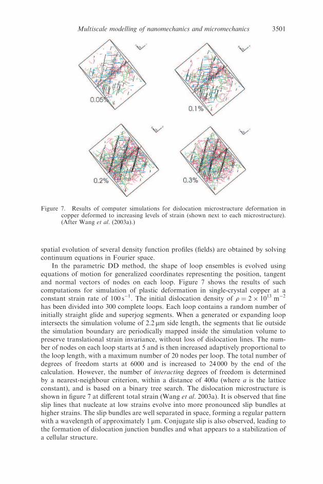
spatial evolution of several density function profiles (fields) are obtained by solvingcontinuum equations in Fourier space.

In the parametric DD method, the shape of loop ensembles is evolved usingequations of motion for generalized coordinates representing the position, tangentand normal vectors of nodes on each loop. Figure 7 shows the results of suchcomputations for simulation of plastic deformation in single-crystal copper at aconstant strain rate of 100 s�1. The initial dislocation density of � ¼ 2� 1013 m�2

has been divided into 300 complete loops. Each loop contains a random number ofinitially straight glide and superjog segments. When a generated or expanding loopintersects the simulation volume of 2.2 mm side length, the segments that lie outsidethe simulation boundary are periodically mapped inside the simulation volume topreserve translational strain invariance, without loss of dislocation lines. The num-ber of nodes on each loop starts at 5 and is then increased adaptively proportional tothe loop length, with a maximum number of 20 nodes per loop. The total number ofdegrees of freedom starts at 6000 and is increased to 24 000 by the end of thecalculation. However, the number of interacting degrees of freedom is determinedby a nearest-neighbour criterion, within a distance of 400a (where a is the latticeconstant), and is based on a binary tree search. The dislocation microstructure isshown in figure 7 at different total strain (Wang et al. 2003a). It is observed that fineslip lines that nucleate at low strains evolve into more pronounced slip bundles athigher strains. The slip bundles are well separated in space, forming a regular patternwith a wavelength of approximately 1 mm. Conjugate slip is also observed, leading tothe formation of dislocation junction bundles and what appears to a stabilization ofa cellular structure.


Figure 7. Results of computer simulations for dislocation microstructure deformation incopper deformed to increasing levels of strain (shown next to each microstructure).(After Wang et al. (2003a).)

4.4. Statistical mechanicsTwo of the most fascinating features of microscale plasticity are the spontaneous

formation of dislocation patterns, and the highly intermittent and spatially localizednature of plastic flow. Dislocation patterns consist of alternating dislocation-richand dislocation-poor regions usually in the micrometre range (e.g. dislocation cells,subgrains, bundles, veins, walls and channels). On the other hand, the local valuesof strain rates associated with intermittent dislocation avalanches are estimated tobe of the order of (1–10)�106 times greater than externally imposed strain rates(Neuhauser 1983, Zaiser 2001). Understanding such collective phenomena is ofparamount importance in two respects.

(i) It will allow materials design approaches that are more fundamentallybased to mitigate the detrimental effects of plastic deformation, fatigue andfracture on material failure.

(ii) It will shed light on the intriguing physics of both self-organizationphenomena and the behaviour of critical-state systems (e.g. avalanches andpercolation).

Because of the high density of dislocations and the strong nature of interactions,direct computer simulations of inhomogeneous plastic deformation and dislocationpatterns are still unattainable. Even if direct computer simulations are successfulin the description of these collective phenomena, it is very desirable to obtainglobal kinetic or thermodynamic principles for understanding the self-organizationassociated with plasticity on the microscale. To attain these objectives, and to enablea direct link with continuum deformation theory, the SM approach has beenadvanced (Neumann 1971, Walgraef and Aifantis 1985, Ghoniem et al. 1990,Gregor and Kratochvil 1990, Kratochvil and Saxlova 1992, Hahner 1996, Saxlovaet al. 1997, Zaiser and Hahner 1997, Hahner et al. 1998, Zaiser et al. 1998,El-Azab 2000, Thomson et al. 2002, LeSar and Richman 2003). The fundamentaldifficulty here is that dislocations, unlike particles, are linear objects of considerabletopological complexity. Hence, when concepts of statistical mechanics and thetheory of rate processes are used, some level of phenomenological description isunavoidable.

Statistical models of dislocation cells, PSBs, shear bands or other organizeddislocation structures attempt to develop continuum equations for dislocation den-sities that contain spatial gradients that drive instabilities and self-organization.Several models have been recently advanced, and will be reviewed briefly here.

The Walgraef–Aifantis (1985) statistical model has gained interest, because ofits ability to predict dislocation pattern formation under cyclic deformation. Themodel is formulated as a set of reaction–diffusion equations with spatial derivativesthat lead to inhomogeneous dislocation distributions and will thus be consideredfirst here. In this model, the static dislocation density, formed by the immobilizeddislocations of the forest, subgrain walls or boundaries, is defined as �s, and themobile dislocation density for dislocations gliding between obstacles is defined as �m.For simplicity, consider systems oriented for single slip. Hence, the mobile disloca-tion density �m is divided into two subfamily densities representing dislocationsgliding in the direction of the Burgers vector (�þm) or in the opposite direction(��m) (with �m ¼ �þm þ ��m). These dislocation densities are related to the strainrate via the Orowan relation _�� ¼ b�mvg, where b is the length of Burgers vector,�m the total mobile dislocation density and vg the glide velocity in the primary


slip plane. Moreover, the dislocation densities are related to the internal stress by therelation

�i ¼�b

2p�þ �b �1=2s ð29Þ

where � is the shear modulus and is a constant. In the last equation, the firstcontribution comes from obstacles such as precipitates or pre-existing walls sepa-rated by an effective spacing � and, the second part is the contribution from the staticdislocation population which also opposes dislocation motion. The internal stress �ireduces the effective stress �e defined as �e ¼ �a � �i, with �a representing the appliedstress. Finally, the glide velocity is related to the effective stress via appropriatephenomenological relations expressing the fact that individual dislocation motionis initiated when the effective stress acting on a dislocation exceeds the yield stress,in the form vg / ð�e=�0Þ

m. This can be put more explicitly as

vg ¼ v0 exp ��

kT

�e�0

� ��m , ð30Þ

where �0 is the yield stress and m > 1. The essential features of DD are theirmobility, which includes thermal diffusion and climb, and their mutual interactionprocesses. By taking into account these mechanisms, the resulting dynamic systemcan be written as (Walgraef and Aifantis 1985)

ot�s ¼ �= � Js þ vg�m�1=2s � vsd�

2s � vg��m�s � �s þ vgGð�sÞ�m,

ot�þm ¼ �= � Jþ þ

2�s � vgGð�sÞ�

þm � vg��

þmð�s þ �

�mÞ,

ot��m ¼ �= � J� þ

2�s � vgGð�sÞ�

�m � vg��

�mð�s þ �

þmÞ,

ð31Þ

where � is the characteristic separation length between dislocations for spontaneousannihilation (Essmann and Mughrabi 1979), d is the characteristic length of sponta-neous dipole collapse, is the frequency of a dislocation freeing from the forest andis proportional to vg= �dd where �dd is the characteristic dipole destabilization lengthwhich is inversely proportional to the effective stress, and ¼ 0vg�e. The differentcharacteristic lengths introduced here, or at least their order of magnitude, may inprinciple be evaluated from microscopic analysis (Neumann 1971, Essmann andMughrabi 1979). Because of mutual interactions, thermal activation and climb,the forest dislocations mobility is represented by a diffusive current J ¼ �Ds=�s,which represents the effective diffusion within the forest. The current of mobiledislocations is taken as J ¼ vg�

m and represents the flux caused by gliding dis-

locations, in the present case, it is the flux caused by their edge component. Stabilityand numerical analyses of the previous set of equations have provided informationon the conditions for formation of PSBs in fatigued specimens. It is shown that PSBformation is triggered by the clustering of dislocations or dislocation dipoles, whichbecome finally immobile and arrange themselves in regularly spaced walls of highdislocation density (Walgraef and Aifantis 1985).

Another class of models is based on the evolution of dipolar loops, triggered bytheir interaction with gliding dislocations (Kratochvil and Saxlova 1992, Saxlovaet al. 1997, Kubin and Kratochvil 2000). The proposed statistical models are of thereaction–transport type and focus on the feedback between the evolution of glidedislocations and the dipole density, as conceptualized earlier by Mughrabi (1981).


The result is the sweeping of dipole loops by screw dislocations, which initiates theformation of dislocation walls. In this approach, dipole generation and interactionsplay a secondary role and are introduced in an ad hoc and qualitative way.

To illustrate briefly the statistical approach of Kratochvil and co-workers, let usconsider N loops of one type (i.e. either interstitial or vacancy), i ¼ 1, . . . ,N. For theith loop, the equation of motion can be then expressed as

dridt

¼ BXNj 6¼i

f intðri � rjÞ þ fext

!, ð32Þ

where B is the loop mobility, fext is the force caused by stress gradients and glidedislocations and f int is the interaction force between dipoles. In order to obtain acontinuous field description, equation (32) is multiplied by the delta function�ðr� riÞ, and the result is differentiated with respect to r; thus we have

d

dr

dridt�ðr� riÞ

� �¼ B

d

dr

XNi¼1

f intðri � rjÞ þ fext

!�ðr� riÞ

" #: ð33Þ

By introduction of the discrete density function %ðr, r1, . . . , rNÞ ¼PN

j 6¼i �ðr� riÞ, andtaking the sum on the right-hand side of equation (33), it can be replaced by aweighted integral. Summing the above equation for all loops, one obtains

d

dt%ðrÞ þ

d

drBfðrÞ%ðrÞ½ � ¼ 0, ð34Þ

where

fðrÞ �

ðf intðs� rÞ%ðsÞ dsþ fext: ð35Þ

As a first approximation it can be assumed that % in equation (34) and definition(35) represents the local averaged loop density %ðrÞ independent of detailed looppositions ri. Then, equation (34) represents the balance equation for the continuousdistribution of loops described by the density %ðrÞ. Since the interaction forcebetween loops fint is short range, Kratochvil and co-workers utilized a Taylor seriesexpansion of %ðrÞ around r to obtain finally

fðrÞ ¼ �d%ðrÞ

dr

ððs� rÞfintðs� rÞdsþ fext: ð36Þ

From the balance equation (34) and approximation (36), the problem of loop–loop interaction was shown to be represented as a diffusion equation in a drift field:

d

dt%ðrÞ ¼

d

drDd%ðrÞ

dr

� �þ

d

drfext, ð37Þ

where D is an effective diffusion coefficient, given by

D ¼ B%ðrÞ

ðsEf intðsÞ ds: ð38Þ

When the motion of screw dislocations is coupled with equation (37), self-organized patterns of dipolar loops may be attainable, as conjectured by Mughrabi(1981).

In an attempt to generalize the statistical description of dislocations, El-Azab(2000) described the dislocation content of a slip system by introducing the distribu-tion �ðiÞðx, v, t, tÞ. Considering only glide motion, the tangent vector is described


by a single scalar parameter: t ¼ tð�Þ. The distribution function �ðiÞ is defined in ageneralized phase space, such that �ðiÞðx, v, �, tÞ dxdv d� is the dislocation line lengthcontained in the phase space volume dxdv d� at time t on the ith slip system. Theapproach of El-Azab (2000) is to consider the conservation equation of the disloca-tion density tensor a, for which dislocations on the ith slip system contribute:

aðiÞðx, tÞ ¼

ðv

ð�

t� bðiÞ�ðiÞðx, v, �, tÞ dv d�: ð39Þ

The condition of compatibility of the total distortion field in the crystal is writtenas aþ =� bP ¼ 0 (Kroner 1981). Considering a volume O, this can be extended to

A ¼

ðOa dOþ

ðO=� bP dO ¼ 0: ð40Þ

P is the plastic distortion tensor. Equation (40) corresponds to the principle ofinvariance of the total Burgers vector. For interacting dislocations, however,El-Azab (2000) included additional source terms to the conservation equations.Thus, for the ith slip system we have

d

dt

ðOaðiÞ dO

� �¼

ðO

XSðiÞ dO , i ¼ 1,N: ð41ÞP

SðiÞ includes all possible tensorial sources SðiÞ resulting from Burgers vector reac-

tions and cross-slip. The time rate of variation in the dislocation density tensor interms of the distribution function has been worked out by El-Azab (2000) as

d

dt

ðx

aðiÞðx, tÞ dx

� �¼

ðx

ðv

ð�

t� bðiÞ o

otþ v � =þ _vv � =v

� ��ðiÞ dxdv d�, ð42Þ

where the terms containing _�� o=o� cancel each other. The right-hand side of equation(41) can also be represented by a phase space integral of scalar source functionsð

O

XSðiÞ dO ¼

ðx

ðv

ð�

t� bðiÞX

SðiÞ dx dv d�: ð43Þ

From the last two equations, El-Azab (2000) finally obtained a set of kinetic equa-tions, of the form

o

otþ v � =þ _vv � =v

� ��ðiÞ ¼

XSðiÞ, i ¼ 1,N: ð44Þ

It is also shown that this generalized approach can be reduced to the more simplifiedformulation of Groma (1997) in the special case of a system of parallel edge disloca-tions in a single-slip configuration. The linear stability analysis of Groma (1997)shows that a homogeneous stationary solution is unstable and that density perturba-tions grow, leading to pattern formation.

In an effort to connect DD simulations to continuum theories, Hartley (2003)introduced the concept of a dislocation distribution vector, defined as

q ðtÞ � t� ðtÞ ð45Þ

so that the magnitude of q ðtÞ is

j q ðtÞj ¼ q ðtÞ, ð46Þ


which is the total length per unit volume of dislocation lines with tangents parallelto t, and with Burgers vector b . The dislocation distribution vector is related tothe Nye tensor a, by

a ¼X

b � q , ð47Þ

where the sum is carried over all Burgers vectors in all slip systems. The curvaturetensor of the deformed volume is given by

j ¼ 12Tr ðaÞ I� a: ð48Þ

Thus, it may be possible to compute the volumetric distortions associated withthe movement of dislocations within a simulation volume, and then connect thesedistortions to continuum theories.

Zaiser (2001) noted that, because of the highly intermittent nature of plastic flow,the instantaneous active slip volume in fcc metals is of the order of 10�6 only andthat, at typical strain rates of 10�4 s�1, the time between neighbouring avalanchesexceeds the lifetime of an individual avalanche by four to six orders of magnitude.On that basis, he concluded that plastic deformation can be characterized as a slowlydriven non-equilibrium system exhibiting large fluctuations. To estimate the magni-tude of such fluctuations, Hahner (1996) proposed that, if one neglects dislocationmultiplication and annihilation, the average work done by the internal stress must bezero, and that the work of the external stress is dissipated into heat. Thus, one canwrite

� intv

D E¼ 0, ð49Þ

where � int and v are internal stresses and dislocation velocities on slip system .Recognizing that the effective stress �eff has an external �ext plus an internal �intcomponent, and upon separating the stress and velocity into average (representedby h� � �i) and fluctuating (represented by d � � �) components, Zaiser (2001) arrives atthe following expressions for the autocorrelation functions of the effective stress � eff ,and dislocation velocity v fluctuations:

ðd� eff Þ2

D E¼ � int

D E� eff

D E,

ðdv Þ2� �v � �2 ¼

� int

D E� eff

D E ¼ b2� � int

D EB _�� ,

ð50Þ

where B is the mobility, and _�� is the average shear strain rate. Using typical valuesfor copper in the previous equations, the relative velocity fluctuation is found to beof the order of 107 Zaiser (2001) in accordance with the experimental measurementsof Neuhauser (1983).

Recently, detailed measurements of the misorientation angles across dislocationwalls have been made by Hughes et al. (1998). Zaiser (2001) formulated a velocity-averaged stochastic version of equation (44) for the distribution function of surplusdislocation segments or geometrically necessary dislocations to show that the prob-ability distribution function for misorientation angles is in good agreement with theexperimental measurements of Hughes et al. (1998).


A percolation-type stochastic dislocation model has been advanced by Thomsonand co-workers (Thomson and Levine 1998, Shim et al. 2001, Thomson et al. 2002).In this model, which is limited to stage III deformation, the weakest cell in a bandundergoes a burst of strain, which initiates a cluster of newly strained cells. Sliptransmission to neighbouring cells is assumed to be of the form s� ¼ as, where s is thenumber of dislocations in the strained cell, a is a pile-up amplification factor and s� isthe number of dislocations in the previously unstrained cell. The key parameter a insuch a model is assumed to depend on two types of mechanisms: firstly, a randomdistribution of sources within the cell walls and/or, secondly a distribution of locksholding up dislocations within the cell walls. Their analysis shows that percolatingslip clusters conform to the universality class of percolation theory (Stauffer andAharony 1992). Furthermore, it can be effectively used to describe slip transmissionin stage III, and that a well-defined percolation threshold can be identified.

The power of SM can be brought to bear on one of the most important chal-lenges for the multiscale modelling approach. The large disparity in time and lengthscales during plastic deformation limit the reach of direct DD simulations. Hence, itis of interest to determine the necessary coarse-graining strategies for both temporaland spatial variables. LeSar and co-workers (Lesar et al. 1989, LeSar and Rickman2002, 2003, Rickman et al. 2003) have begun to tackle this issue by investigations ofa number of specific problems, namely the combined motion of dislocations andsolutes, and the problem of the long-range interactions of blocks of dislocationensembles.

In the limit where the solute mobility is high relative to that of dislocations,dislocation–solute atmosphere pairs can be treated as quasi-particles, and thedegrees of freedom associated with individual solute atoms can be eliminated(Rickman et al. 2003). Thus, an effective mobility can be derived and can be relatedto the details of such interaction. However, in the other extreme limit of low solutemobility compared with dislocations, the solute atoms function essentially asstatic traps for dislocations. In this case, LeSar and co-workers modelled slip as adiscrete one-dimensional ‘birth-and-death’ stochastic process (Van Kampen 1992).LeSar and Rickman (2003) found that the dislocation diffusivity is modified by�Dðc, �=kBTÞ:

�D

D0¼ �c

�t=� � 1

c �t=� � 1ð Þ þ 1, ð51Þ

where �t=� ¼ exp ��=kBTð Þ is the mean residence time in a trapped state, D0 is thediffusivity when there are no traps, c � Nt=N is the trap (i.e. solute) concentration.These examples show that it may be possible to average out fast time variables in DDsimulations.

The issue of spatial averaging has been recently dealt with by LeSar andRickman (2002) and Wang et al. (2003b). Starting from the work of Kossevich(1979) on the interaction energy of systems of dislocations, an energy expressionin terms of the dislocation density tensor (Rickman et al. 2003) is derived. The basicidea in this approach is to divide space into small averaging volumes to calculate thelocal multipole moments of the dislocation microstructure and then to write theenergy (LeSar and Rickman 2002) or the force (Wang et al. 2003b) as an expansionover the multipoles. Numerical implementation of the multipole expansion for thePeach–Kohler force on a test dislocation separated from a volume containing adense dislocation aggregate revealed that such a technique is highly accurate and


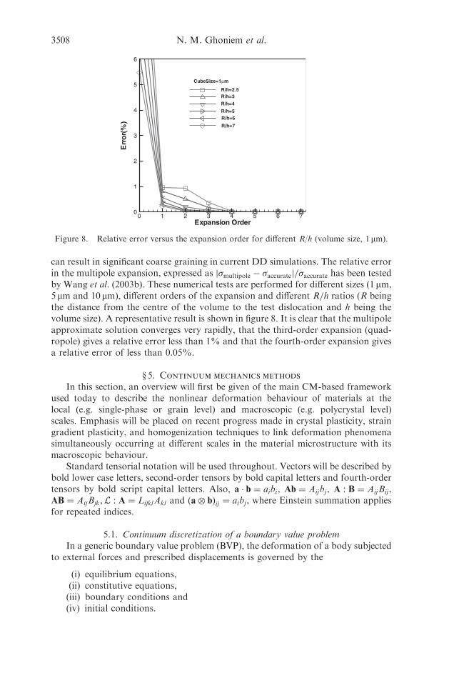
can result in significant coarse graining in current DD simulations. The relative errorin the multipole expansion, expressed as j�multipole � �accuratej=�accurate has been testedby Wang et al. (2003b). These numerical tests are performed for different sizes (1 mm,5 mm and 10 mm), different orders of the expansion and different R=h ratios (R beingthe distance from the centre of the volume to the test dislocation and h being thevolume size). A representative result is shown in figure 8. It is clear that the multipoleapproximate solution converges very rapidly, that the third-order expansion (quad-ropole) gives a relative error less than 1% and that the fourth-order expansion givesa relative error of less than 0:05%.

} 5. Continuum mechanics methods

In this section, an overview will first be given of the main CM-based frameworkused today to describe the nonlinear deformation behaviour of materials at thelocal (e.g. single-phase or grain level) and macroscopic (e.g. polycrystal level)scales. Emphasis will be placed on recent progress made in crystal plasticity, straingradient plasticity, and homogenization techniques to link deformation phenomenasimultaneously occurring at different scales in the material microstructure with itsmacroscopic behaviour.

Standard tensorial notation will be used throughout. Vectors will be described bybold lower case letters, second-order tensors by bold capital letters and fourth-ordertensors by bold script capital letters. Also, a � b ¼ aibi, Ab ¼ Aijbj, A : B ¼ AijBij ,AB ¼ AijBjk,L : A ¼ LijklAkl and ða� bÞij ¼ aibj, where Einstein summation appliesfor repeated indices.

5.1. Continuum discretization of a boundary value problemIn a generic boundary value problem (BVP), the deformation of a body subjected

to external forces and prescribed displacements is governed by the

(i) equilibrium equations,(ii) constitutive equations,(iii) boundary conditions and(iv) initial conditions.


Expansion Order

Err

or(

%)

0 1 2 3 4 5 6 70

1

2

3

4

5

6

R/h=2.5R/h=3

R/h=4

R/h=5R/h=6

R/h=7

CubeSize=1µm

Figure 8. Relative error versus the expansion order for different R/h (volume size, 1mm).

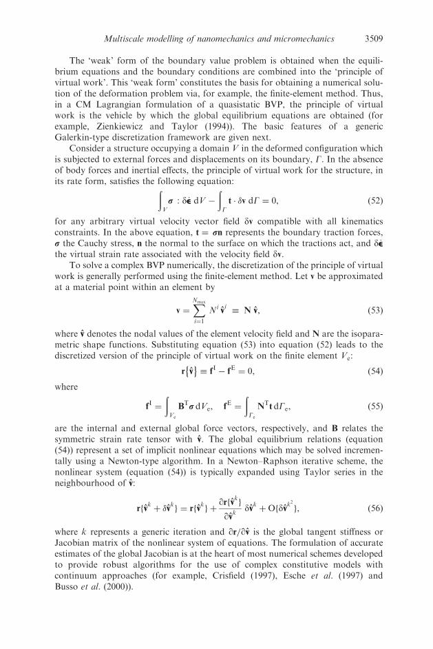
The ‘weak’ form of the boundary value problem is obtained when the equili-brium equations and the boundary conditions are combined into the ‘principle ofvirtual work’. This ‘weak form’ constitutes the basis for obtaining a numerical solu-tion of the deformation problem via, for example, the finite-element method. Thus,in a CM Lagrangian formulation of a quasistatic BVP, the principle of virtualwork is the vehicle by which the global equilibrium equations are obtained (forexample, Zienkiewicz and Taylor (1994)). The basic features of a genericGalerkin-type discretization framework are given next.

Consider a structure occupying a domain V in the deformed configuration whichis subjected to external forces and displacements on its boundary, G. In the absenceof body forces and inertial effects, the principle of virtual work for the structure, inits rate form, satisfies the following equation:ð

V

r : d_ee dV �

ðGt � �v dG ¼ 0, ð52Þ

for any arbitrary virtual velocity vector field dv compatible with all kinematicsconstraints. In the above equation, t ¼ rn represents the boundary traction forces,r the Cauchy stress, n the normal to the surface on which the tractions act, and d_eethe virtual strain rate associated with the velocity field dv.

To solve a complex BVP numerically, the discretization of the principle of virtualwork is generally performed using the finite-element method. Let v be approximatedat a material point within an element by

v ¼XNmax

i¼1

Nivvi� N vv, ð53Þ

where vv denotes the nodal values of the element velocity field and N are the isopara-metric shape functions. Substituting equation (53) into equation (52) leads to thediscretized version of the principle of virtual work on the finite element Ve:

r vv �

� fI� f

E¼ 0, ð54Þ

where

fI¼

ðVe

BTr dVe, f

E¼

ðGe

NTt dGe, ð55Þ

are the internal and external global force vectors, respectively, and B relates thesymmetric strain rate tensor with vv. The global equilibrium relations (equation(54)) represent a set of implicit nonlinear equations which may be solved incremen-tally using a Newton-type algorithm. In a Newton–Raphson iterative scheme, thenonlinear system (equation (54)) is typically expanded using Taylor series in theneighbourhood of vv:

rfvvkþ �vv

kg ¼ rfvv

kg þ

orfvvkg

ovvk

dvvk þOfdvvk2

g, ð56Þ

where k represents a generic iteration and or=ovv is the global tangent stiffness orJacobian matrix of the nonlinear system of equations. The formulation of accurateestimates of the global Jacobian is at the heart of most numerical schemes developedto provide robust algorithms for the use of complex constitutive models withcontinuum approaches (for example, Crisfield (1997), Esche et al. (1997) andBusso et al. (2000)).


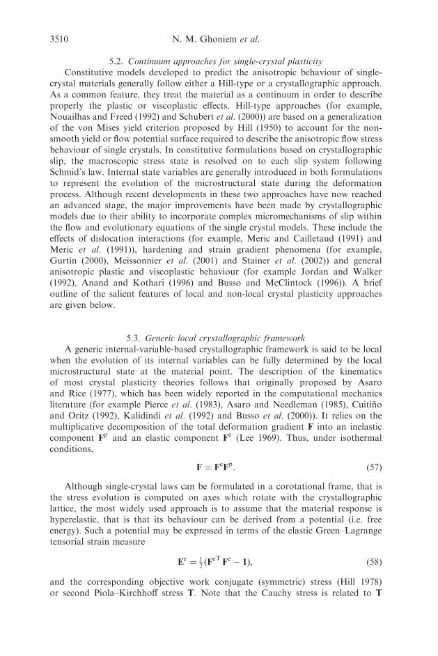
5.2. Continuum approaches for single-crystal plasticityConstitutive models developed to predict the anisotropic behaviour of single-

crystal materials generally follow either a Hill-type or a crystallographic approach.As a common feature, they treat the material as a continuum in order to describeproperly the plastic or viscoplastic effects. Hill-type approaches (for example,Nouailhas and Freed (1992) and Schubert et al. (2000)) are based on a generalizationof the von Mises yield criterion proposed by Hill (1950) to account for the non-smooth yield or flow potential surface required to describe the anisotropic flow stressbehaviour of single crystals. In constitutive formulations based on crystallographicslip, the macroscopic stress state is resolved on to each slip system followingSchmid’s law. Internal state variables are generally introduced in both formulationsto represent the evolution of the microstructural state during the deformationprocess. Although recent developments in these two approaches have now reachedan advanced stage, the major improvements have been made by crystallographicmodels due to their ability to incorporate complex micromechanisms of slip withinthe flow and evolutionary equations of the single crystal models. These include theeffects of dislocation interactions (for example, Meric and Cailletaud (1991) andMeric et al. (1991)), hardening and strain gradient phenomena (for example,Gurtin (2000), Meissonnier et al. (2001) and Stainer et al. (2002)) and generalanisotropic plastic and viscoplastic behaviour (for example Jordan and Walker(1992), Anand and Kothari (1996) and Busso and McClintock (1996)). A briefoutline of the salient features of local and non-local crystal plasticity approachesare given below.

5.3. Generic local crystallographic frameworkA generic internal-variable-based crystallographic framework is said to be local

when the evolution of its internal variables can be fully determined by the localmicrostructural state at the material point. The description of the kinematicsof most crystal plasticity theories follows that originally proposed by Asaroand Rice (1977), which has been widely reported in the computational mechanicsliterature (for example Pierce et al. (1983), Asaro and Needleman (1985), Cuitinoand Oritz (1992), Kalidindi et al. (1992) and Busso et al. (2000)). It relies on themultiplicative decomposition of the total deformation gradient F into an inelasticcomponent F

p and an elastic component Fe (Lee 1969). Thus, under isothermal

conditions,

F ¼ FeFp: ð57Þ

Although single-crystal laws can be formulated in a corotational frame, that isthe stress evolution is computed on axes which rotate with the crystallographiclattice, the most widely used approach is to assume that the material response ishyperelastic, that is that its behaviour can be derived from a potential (i.e. freeenergy). Such a potential may be expressed in terms of the elastic Green–Lagrangetensorial strain measure

Ee¼ 1

2ðF

eTFe� 1Þ, ð58Þ

and the corresponding objective work conjugate (symmetric) stress (Hill 1978)or second Piola–Kirchhoff stress T. Note that the Cauchy stress is related to T


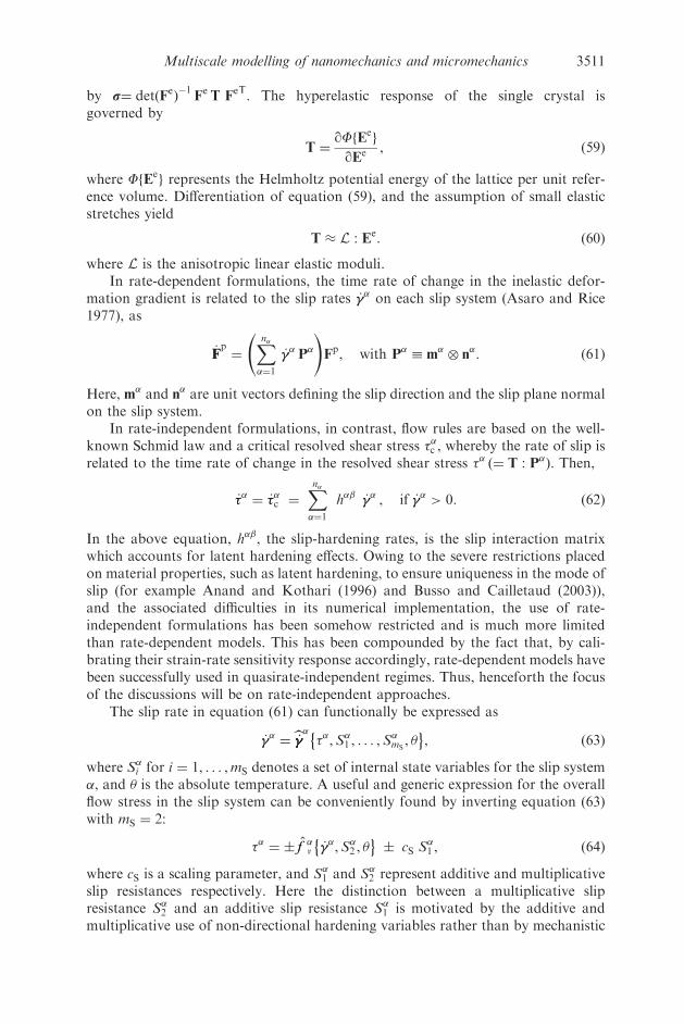
by r¼ detðFeÞ�1

FeT F

eT. The hyperelastic response of the single crystal isgoverned by

T ¼oFfEe

g

oEe , ð59Þ

where FfEeg represents the Helmholtz potential energy of the lattice per unit refer-

ence volume. Differentiation of equation (59), and the assumption of small elasticstretches yield

T L : Ee: ð60Þ

where L is the anisotropic linear elastic moduli.In rate-dependent formulations, the time rate of change in the inelastic defor-

mation gradient is related to the slip rates _�� on each slip system (Asaro and Rice1977), as

_FFp¼

Xn��¼1

_�� P�

!Fp, with P

�� m

�� n

�: ð61Þ

Here, m� and n� are unit vectors defining the slip direction and the slip plane normal

on the slip system.In rate-independent formulations, in contrast, flow rules are based on the well-

known Schmid law and a critical resolved shear stress ��c , whereby the rate of slip isrelated to the time rate of change in the resolved shear stress �� ð¼ T : P�Þ. Then,

_�� ¼ _��c ¼Xn��¼1

h� _�� , if _�� > 0: ð62Þ

In the above equation, h� , the slip-hardening rates, is the slip interaction matrixwhich accounts for latent hardening effects. Owing to the severe restrictions placedon material properties, such as latent hardening, to ensure uniqueness in the mode ofslip (for example Anand and Kothari (1996) and Busso and Cailletaud (2003)),and the associated difficulties in its numerical implementation, the use of rate-independent formulations has been somehow restricted and is much more limitedthan rate-dependent models. This has been compounded by the fact that, by cali-brating their strain-rate sensitivity response accordingly, rate-dependent models havebeen successfully used in quasirate-independent regimes. Thus, henceforth the focusof the discussions will be on rate-independent approaches.

The slip rate in equation (61) can functionally be expressed as

_�� ¼b_��_�� ,S�1 , . . . ,S�mS, �

�, ð63Þ

where S�i for i ¼ 1, . . . ,mS denotes a set of internal state variables for the slip system�, and � is the absolute temperature. A useful and generic expression for the overallflow stress in the slip system can be conveniently found by inverting equation (63)with mS ¼ 2:

�� ¼ ff �v _��,S�2 , � �

cS S�1 , ð64Þ

where cS is a scaling parameter, and S�1 and S�2 represent additive and multiplicativeslip resistances respectively. Here the distinction between a multiplicative slipresistance S�2 and an additive slip resistance S�1 is motivated by the additive andmultiplicative use of non-directional hardening variables rather than by mechanistic


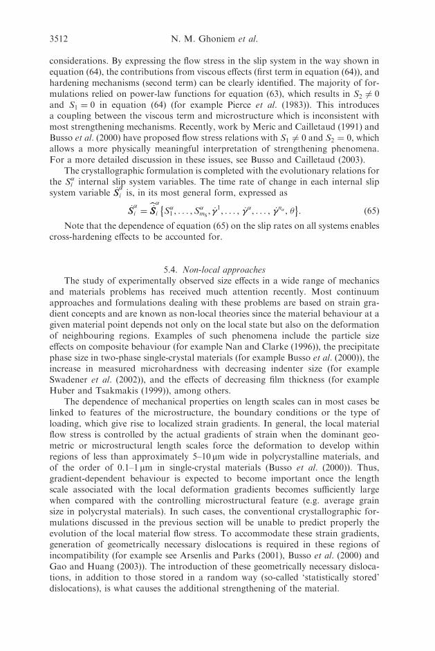
considerations. By expressing the flow stress in the slip system in the way shown inequation (64), the contributions from viscous effects (first term in equation (64)), andhardening mechanisms (second term) can be clearly identified. The majority of for-mulations relied on power-law functions for equation (63), which results in S2 6¼ 0and S1 ¼ 0 in equation (64) (for example Pierce et al. (1983)). This introducesa coupling between the viscous term and microstructure which is inconsistent withmost strengthening mechanisms. Recently, work by Meric and Cailletaud (1991) andBusso et al. (2000) have proposed flow stress relations with S1 6¼ 0 and S2 ¼ 0, whichallows a more physically meaningful interpretation of strengthening phenomena.For a more detailed discussion in these issues, see Busso and Cailletaud (2003).

The crystallographic formulation is completed with the evolutionary relations forthe S�i internal slip system variables. The time rate of change in each internal slipsystem variable _SS

�i is, in its most general form, expressed as

_SS�i ¼

b_SS_SS�i S�1 , . . . ,S�mS, _��1, . . . , _��, . . . , _��n� , �

�: ð65Þ

Note that the dependence of equation (65) on the slip rates on all systems enablescross-hardening effects to be accounted for.

5.4. Non-local approachesThe study of experimentally observed size effects in a wide range of mechanics

and materials problems has received much attention recently. Most continuumapproaches and formulations dealing with these problems are based on strain gra-dient concepts and are known as non-local theories since the material behaviour at agiven material point depends not only on the local state but also on the deformationof neighbouring regions. Examples of such phenomena include the particle sizeeffects on composite behaviour (for example Nan and Clarke (1996)), the precipitatephase size in two-phase single-crystal materials (for example Busso et al. (2000)), theincrease in measured microhardness with decreasing indenter size (for exampleSwadener et al. (2002)), and the effects of decreasing film thickness (for exampleHuber and Tsakmakis (1999)), among others.

The dependence of mechanical properties on length scales can in most cases belinked to features of the microstructure, the boundary conditions or the type ofloading, which give rise to localized strain gradients. In general, the local materialflow stress is controlled by the actual gradients of strain when the dominant geo-metric or microstructural length scales force the deformation to develop withinregions of less than approximately 5–10 mm wide in polycrystalline materials, andof the order of 0.1–1 mm in single-crystal materials (Busso et al. (2000)). Thus,gradient-dependent behaviour is expected to become important once the lengthscale associated with the local deformation gradients becomes sufficiently largewhen compared with the controlling microstructural feature (e.g. average grainsize in polycrystal materials). In such cases, the conventional crystallographic for-mulations discussed in the previous section will be unable to predict properly theevolution of the local material flow stress. To accommodate these strain gradients,generation of geometrically necessary dislocations is required in these regions ofincompatibility (for example see Arsenlis and Parks (2001), Busso et al. (2000) andGao and Huang (2003)). The introduction of these geometrically necessary disloca-tions, in addition to those stored in a random way (so-called ‘statistically stored’dislocations), is what causes the additional strengthening of the material.


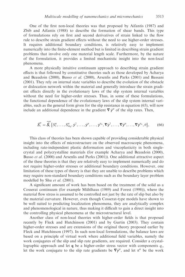
One of the first non-local theories was that proposed by Aifantis (1987) andZbib and Aifantis (1988) to describe the formation of shear bands. This typeof formulations rely on first and second derivatives of strain linked to the flowrule to describe strain gradient effects without the need to use higher-order stresses.It requires additional boundary conditions, is relatively easy to implementnumerically into the finite-element method but is limited in describing strain gradientproblems that involve only one material length scale. Furthermore, by the natureof the formulation, it provides a limited mechanistic insight into the non-localphenomena.

A more physically intuitive continuum approach to describing strain gradienteffects is that followed by constitutive theories such as those developed by Acharyaand Beaudoin (2000), Busso et al. (2000), Arsenlis and Parks (2001) and Bassani(2001). They rely on internal state variables to describe the evolution of the obstacleor dislocation network within the material and generally introduce the strain gradi-ent effects directly in the evolutionary laws of the slip system internal variableswithout the need for higher-order stresses. Thus, in some of these formulations,the functional dependence of the evolutionary laws of the slip system internal vari-ables, such as the general form given for the slip resistance in equation (65), will nowinclude an additional dependence in the gradient = _�� of the slip rates. Then,

_SS�i ¼

b_SS_SS�i S�1 , . . . ,S�mS, _��1, . . . , _��, . . . , _��n� ,= _��1, . . . ,= _��, . . . ,= _��n� , �

�, ð66Þ

This class of theories has been shown capable of providing considerable physicalinsight into the effects of microstructure on the observed macroscopic phenomena,including rate-independent plastic deformation and viscoplasticity in both single-crystal and polycrystalline materials (for example Acharya and Beaudoin (2000),Busso et al. (2000) and Arsenlis and Parks (2001)). One additional attractive aspectof the these theories is that they are relatively easy to implement numerically and donot require higher-order stresses or additional boundary conditions. However, onelimitation of these types of theory is that they are unable to describe problems whichmay require non-standard boundary conditions such as the boundary layer problemmodelled by Shu et al. (2001).

A significant amount of work has been based on the treatment of the solid as aCosserat continuum (for example Muhlhaus (1989) and Forest (1998)), where thematerial flow stress is assumed to be controlled not just by the rate of slip but also bythe material curvature. However, even though Cosserat-type models have shown tobe well suited to predicting localization phenomena, they are analytically complexand phenomenological in nature, thus making it difficult to gain a direct insight intothe controlling physical phenomena at the microstructural level.

Another class of non-local theories with higher-order fields is that proposedrecently by Fleck and Hutchinson (2001) and by Gurtin (2003). They containhigher-order stresses and are extensions of the original theory proposed earlier byFleck and Hutchinson (1997). In such non-local formulations, the balance laws arebased on a principle of virtual work where additional field variables, namely thework conjugates of the slip and slip rate gradients, are required. Consider a crystal-lographic approach and let q be a higher-order stress vector with components qi,let the work conjugate to the slip rate gradients be = _��, and let p� be the work


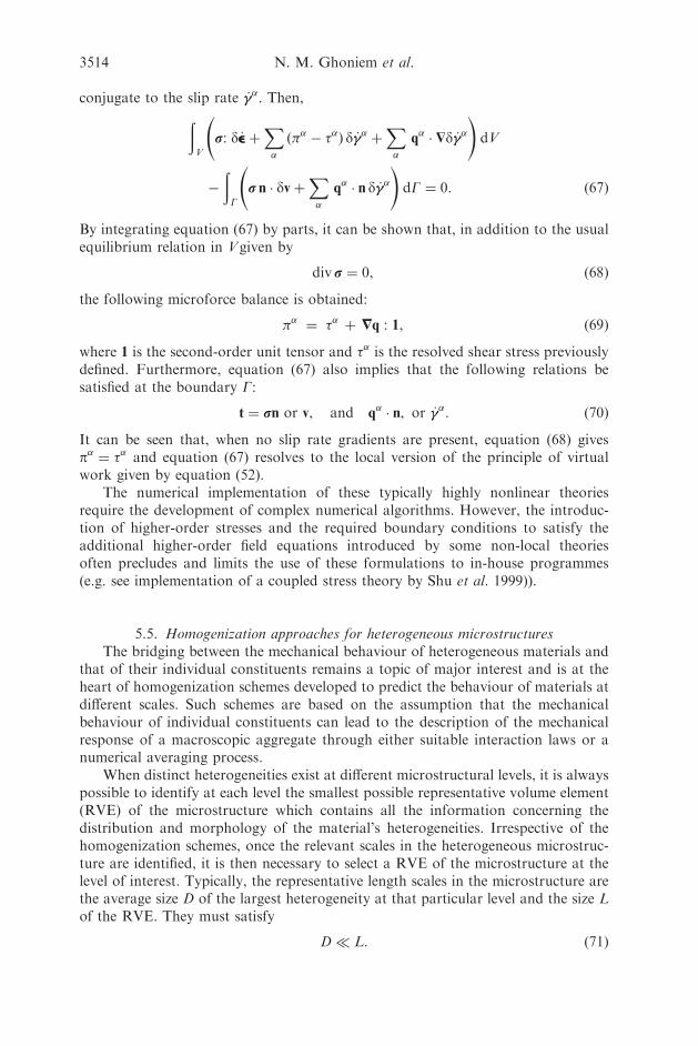
conjugate to the slip rate _��. Then,ðV

r: d_eeþX�

ð�� Þ d _�� þX�

q�� Jd _��

!dV

�

ðG

r n � dvþX�

q�� n d _��

!dG ¼ 0: ð67Þ

By integrating equation (67) by parts, it can be shown that, in addition to the usualequilibrium relation in Vgiven by

div r ¼ 0, ð68Þ

the following microforce balance is obtained:

�� ¼ �� þ =q : 1, ð69Þ

where 1 is the second-order unit tensor and �� is the resolved shear stress previouslydefined. Furthermore, equation (67) also implies that the following relations besatisfied at the boundary G:

t ¼ rn or v, and q�� n, or _��: ð70Þ

It can be seen that, when no slip rate gradients are present, equation (68) givesp� ¼ �� and equation (67) resolves to the local version of the principle of virtualwork given by equation (52).

The numerical implementation of these typically highly nonlinear theoriesrequire the development of complex numerical algorithms. However, the introduc-tion of higher-order stresses and the required boundary conditions to satisfy theadditional higher-order field equations introduced by some non-local theoriesoften precludes and limits the use of these formulations to in-house programmes(e.g. see implementation of a coupled stress theory by Shu et al. 1999)).

5.5. Homogenization approaches for heterogeneous microstructuresThe bridging between the mechanical behaviour of heterogeneous materials and

that of their individual constituents remains a topic of major interest and is at theheart of homogenization schemes developed to predict the behaviour of materials atdifferent scales. Such schemes are based on the assumption that the mechanicalbehaviour of individual constituents can lead to the description of the mechanicalresponse of a macroscopic aggregate through either suitable interaction laws or anumerical averaging process.

When distinct heterogeneities exist at different microstructural levels, it is alwayspossible to identify at each level the smallest possible representative volume element(RVE) of the microstructure which contains all the information concerning thedistribution and morphology of the material’s heterogeneities. Irrespective of thehomogenization schemes, once the relevant scales in the heterogeneous microstruc-ture are identified, it is then necessary to select a RVE of the microstructure at thelevel of interest. Typically, the representative length scales in the microstructure arethe average size D of the largest heterogeneity at that particular level and the size Lof the RVE. They must satisfy

D � L: ð71Þ


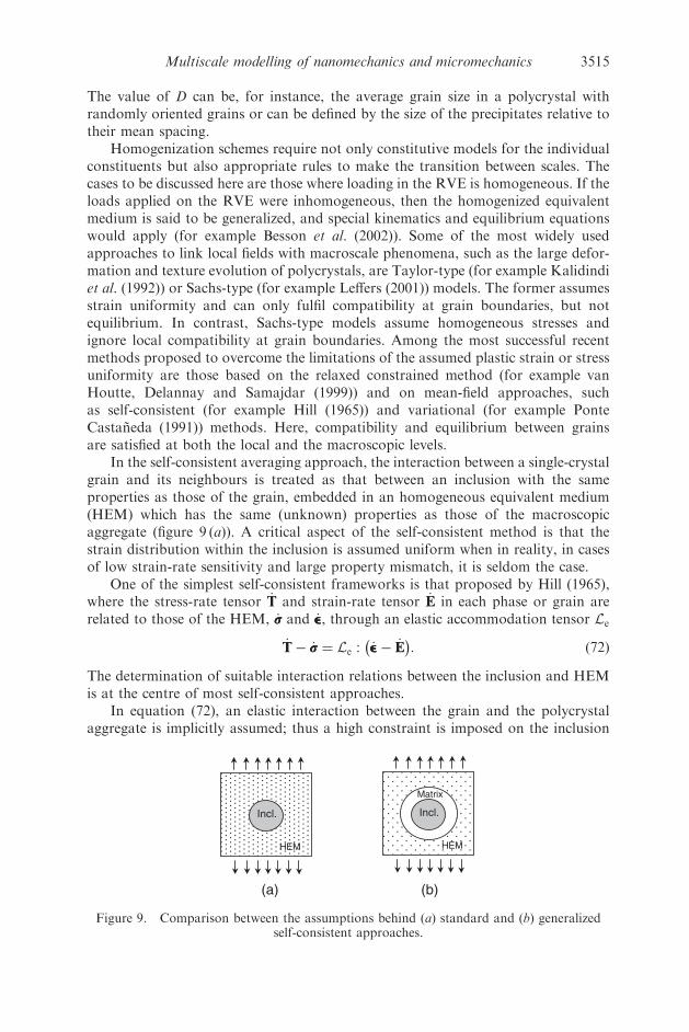
The value of D can be, for instance, the average grain size in a polycrystal withrandomly oriented grains or can be defined by the size of the precipitates relative totheir mean spacing.

Homogenization schemes require not only constitutive models for the individualconstituents but also appropriate rules to make the transition between scales. Thecases to be discussed here are those where loading in the RVE is homogeneous. If theloads applied on the RVE were inhomogeneous, then the homogenized equivalentmedium is said to be generalized, and special kinematics and equilibrium equationswould apply (for example Besson et al. (2002)). Some of the most widely usedapproaches to link local fields with macroscale phenomena, such as the large defor-mation and texture evolution of polycrystals, are Taylor-type (for example Kalidindiet al. (1992)) or Sachs-type (for example Leffers (2001)) models. The former assumesstrain uniformity and can only fulfil compatibility at grain boundaries, but notequilibrium. In contrast, Sachs-type models assume homogeneous stresses andignore local compatibility at grain boundaries. Among the most successful recentmethods proposed to overcome the limitations of the assumed plastic strain or stressuniformity are those based on the relaxed constrained method (for example vanHoutte, Delannay and Samajdar (1999)) and on mean-field approaches, suchas self-consistent (for example Hill (1965)) and variational (for example PonteCastaneda (1991)) methods. Here, compatibility and equilibrium between grainsare satisfied at both the local and the macroscopic levels.

In the self-consistent averaging approach, the interaction between a single-crystalgrain and its neighbours is treated as that between an inclusion with the sameproperties as those of the grain, embedded in an homogeneous equivalent medium(HEM) which has the same (unknown) properties as those of the macroscopicaggregate (figure 9 (a)). A critical aspect of the self-consistent method is that thestrain distribution within the inclusion is assumed uniform when in reality, in casesof low strain-rate sensitivity and large property mismatch, it is seldom the case.

One of the simplest self-consistent frameworks is that proposed by Hill (1965),where the stress-rate tensor _TT and strain-rate tensor _EE in each phase or grain arerelated to those of the HEM, _rr and _ee, through an elastic accommodation tensor Le

_TT� _rr ¼ Le : _ee� _EE� �

: ð72Þ

The determination of suitable interaction relations between the inclusion and HEMis at the centre of most self-consistent approaches.

In equation (72), an elastic interaction between the grain and the polycrystalaggregate is implicitly assumed; thus a high constraint is imposed on the inclusion


HEM

Incl.

HEM

Incl.

Matrix

(a) (b)

Figure 9. Comparison between the assumptions behind (a) standard and (b) generalizedself-consistent approaches.

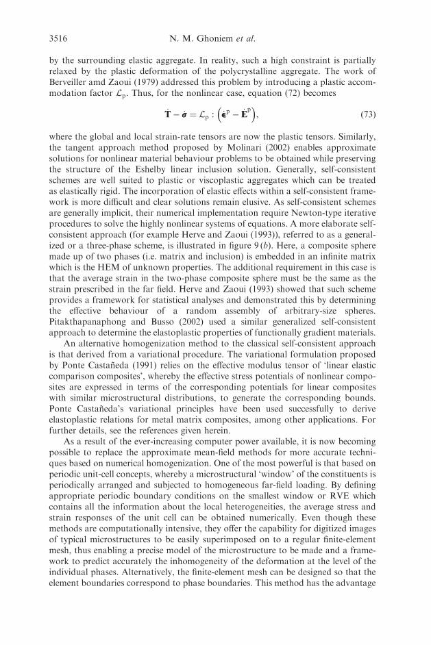
by the surrounding elastic aggregate. In reality, such a high constraint is partiallyrelaxed by the plastic deformation of the polycrystalline aggregate. The work ofBerveiller amd Zaoui (1979) addressed this problem by introducing a plastic accom-modation factor Lp. Thus, for the nonlinear case, equation (72) becomes

_TT� _rr ¼ Lp : _eep � _EEp

� �, ð73Þ

where the global and local strain-rate tensors are now the plastic tensors. Similarly,the tangent approach method proposed by Molinari (2002) enables approximatesolutions for nonlinear material behaviour problems to be obtained while preservingthe structure of the Eshelby linear inclusion solution. Generally, self-consistentschemes are well suited to plastic or viscoplastic aggregates which can be treatedas elastically rigid. The incorporation of elastic effects within a self-consistent frame-work is more difficult and clear solutions remain elusive. As self-consistent schemesare generally implicit, their numerical implementation require Newton-type iterativeprocedures to solve the highly nonlinear systems of equations. A more elaborate self-consistent approach (for example Herve and Zaoui (1993)), referred to as a general-ized or a three-phase scheme, is illustrated in figure 9 (b). Here, a composite spheremade up of two phases (i.e. matrix and inclusion) is embedded in an infinite matrixwhich is the HEM of unknown properties. The additional requirement in this case isthat the average strain in the two-phase composite sphere must be the same as thestrain prescribed in the far field. Herve and Zaoui (1993) showed that such schemeprovides a framework for statistical analyses and demonstrated this by determiningthe effective behaviour of a random assembly of arbitrary-size spheres.Pitakthapanaphong and Busso (2002) used a similar generalized self-consistentapproach to determine the elastoplastic properties of functionally gradient materials.

An alternative homogenization method to the classical self-consistent approachis that derived from a variational procedure. The variational formulation proposedby Ponte Castaneda (1991) relies on the effective modulus tensor of ‘linear elasticcomparison composites’, whereby the effective stress potentials of nonlinear compo-sites are expressed in terms of the corresponding potentials for linear compositeswith similar microstructural distributions, to generate the corresponding bounds.Ponte Castaneda’s variational principles have been used successfully to deriveelastoplastic relations for metal matrix composites, among other applications. Forfurther details, see the references given herein.

As a result of the ever-increasing computer power available, it is now becomingpossible to replace the approximate mean-field methods for more accurate techni-ques based on numerical homogenization. One of the most powerful is that based onperiodic unit-cell concepts, whereby a microstructural ‘window’ of the constituents isperiodically arranged and subjected to homogeneous far-field loading. By definingappropriate periodic boundary conditions on the smallest window or RVE whichcontains all the information about the local heterogeneities, the average stress andstrain responses of the unit cell can be obtained numerically. Even though thesemethods are computationally intensive, they offer the capability for digitized imagesof typical microstructures to be easily superimposed on to a regular finite-elementmesh, thus enabling a precise model of the microstructure to be made and a frame-work to predict accurately the inhomogeneity of the deformation at the level of theindividual phases. Alternatively, the finite-element mesh can be designed so that theelement boundaries correspond to phase boundaries. This method has the advantage


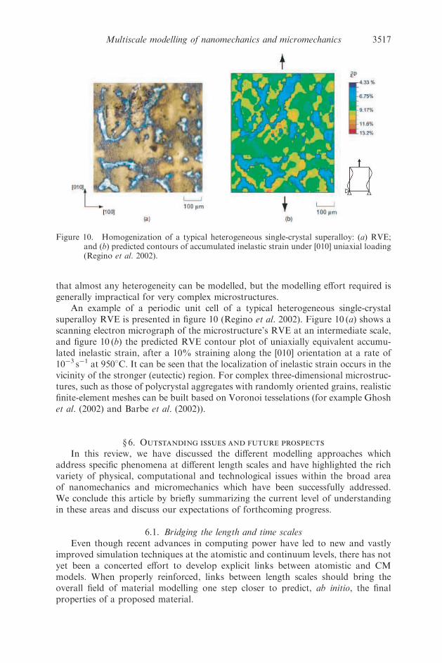
that almost any heterogeneity can be modelled, but the modelling effort required isgenerally impractical for very complex microstructures.

An example of a periodic unit cell of a typical heterogeneous single-crystalsuperalloy RVE is presented in figure 10 (Regino et al. 2002). Figure 10 (a) shows ascanning electron micrograph of the microstructure’s RVE at an intermediate scale,and figure 10 (b) the predicted RVE contour plot of uniaxially equivalent accumu-lated inelastic strain, after a 10% straining along the [010] orientation at a rate of10�3 s�1 at 950�C. It can be seen that the localization of inelastic strain occurs in thevicinity of the stronger (eutectic) region. For complex three-dimensional microstruc-tures, such as those of polycrystal aggregates with randomly oriented grains, realisticfinite-element meshes can be built based on Voronoi tesselations (for example Ghoshet al. (2002) and Barbe et al. (2002)).

} 6. Outstanding issues and future prospects

In this review, we have discussed the different modelling approaches whichaddress specific phenomena at different length scales and have highlighted the richvariety of physical, computational and technological issues within the broad areaof nanomechanics and micromechanics which have been successfully addressed.We conclude this article by briefly summarizing the current level of understandingin these areas and discuss our expectations of forthcoming progress.

6.1. Bridging the length and time scalesEven though recent advances in computing power have led to new and vastly

improved simulation techniques at the atomistic and continuum levels, there has notyet been a concerted effort to develop explicit links between atomistic and CMmodels. When properly reinforced, links between length scales should bring theoverall field of material modelling one step closer to predict, ab initio, the finalproperties of a proposed material.


Figure 10. Homogenization of a typical heterogeneous single-crystal superalloy: (a) RVE;and (b) predicted contours of accumulated inelastic strain under [010] uniaxial loading(Regino et al. 2002).

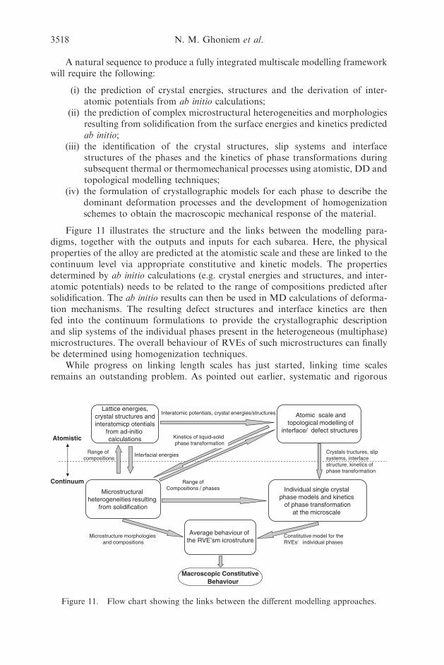
A natural sequence to produce a fully integrated multiscale modelling frameworkwill require the following:

(i) the prediction of crystal energies, structures and the derivation of inter-atomic potentials from ab initio calculations;

(ii) the prediction of complex microstructural heterogeneities and morphologiesresulting from solidification from the surface energies and kinetics predictedab initio;

(iii) the identification of the crystal structures, slip systems and interfacestructures of the phases and the kinetics of phase transformations duringsubsequent thermal or thermomechanical processes using atomistic, DD andtopological modelling techniques;

(iv) the formulation of crystallographic models for each phase to describe thedominant deformation processes and the development of homogenizationschemes to obtain the macroscopic mechanical response of the material.

Figure 11 illustrates the structure and the links between the modelling para-digms, together with the outputs and inputs for each subarea. Here, the physicalproperties of the alloy are predicted at the atomistic scale and these are linked to thecontinuum level via appropriate constitutive and kinetic models. The propertiesdetermined by ab initio calculations (e.g. crystal energies and structures, and inter-atomic potentials) needs to be related to the range of compositions predicted aftersolidification. The ab initio results can then be used in MD calculations of deforma-tion mechanisms. The resulting defect structures and interface kinetics are thenfed into the continuum formulations to provide the crystallographic descriptionand slip systems of the individual phases present in the heterogeneous (multiphase)microstructures. The overall behaviour of RVEs of such microstructures can finallybe determined using homogenization techniques.

While progress on linking length scales has just started, linking time scalesremains an outstanding problem. As pointed out earlier, systematic and rigorous


Lattice energies,crystal structures andinteratomicp otentials

from ad-initiocalculations

Atomic scale andtopological modelling of

interface/ defect structures

Microstructuralheterogeneities resulting

from solidification

Individual single crystalphase models and kinetics

of phase transformationat the microscale

Average behaviour ofthe RVE’sm icrostruture

Interatomic potentials, crystal energies/structures

Interfacial energiesRange ofcompositions

Crystals tructures, slipsystems, interfacestructure, kinetics ofphase transformation

Range ofCompositions / phases

Microstructure morphologiesand compositions

Constitutive model for theRVEs' individual phases

Kinetics of liquid-solidphase transformation

Macroscopic ConstitutiveBehaviour

Atomistic

Continuum

Figure 11. Flow chart showing the links between the different modelling approaches.

reduction in the degrees of freedom that describe material evolution will lead toself-consistent length scale linking, and hence confident predictions of mechanicalproperties. On the other hand, methods for self-consistent linking of time scales arestill lacking. Events at the atomic scale are often in the picosecond to nanosecondrange, while microstructure evolution takes place on much longer time scales:seconds to years. Since the time evolution of the microstructure is path dependent,events that occur in the picosecond to nanosecond time scale (e.g. atomic jumps andnucleation) may have profound effects on microstructure evolution. In addition,relaxation time scales in atomic models cannot be matched by continuum relaxationtime scales. Thus, when a MD model is directly linked to the continuum, matchingcan be accomplished for static or quasistatic problems, while it has not been shownfor fully dynamic problems. Progress in this area is needed.

6.2. Atomistic scalesAtomistic simulations have mainly supplemented experimentally obtained infor-

mation until now. Nevertheless, future developments are expected in four majordirections:

(i) higher accuracy;(ii) larger systems;(iii) computationally faster methods; and(iv) more general approaches.

Density functional approaches have evolved rather rapidly during the pastdecade to address accuracy. The introduction of generalized gradient correctionshas improved the accuracy of binding energies, surface energies and energy barriers.While the standard local spin density and generalized gradient approximations forthe exchange–correlation energy can work for certain cases of strong correlation,that is where electrons partially preserve their localized atomic-like nature, theyfail dramatically for others. Novel functionals, such as the recently developedself-correlation-free meta-GGA and self-interaction-free hyper-GGA, might yielda more reliable description of strong correlations. It is also possible that the useof quantum MC methods for benchmark calculations could provide a fruitful pathto assess and improve density functionals. Concurrent with the above effortsin developing more accurate functionals within the spirit of DFT, several othermethods have been recently developed to treat the ground-state properties ofcondensed systems that exhibit strong correlations. As alluded to in } 2, these includethe self-interaction correction method, the LDAþU method, the LDAþdynamicmean-field theory method, and the optimized effective potential method. In addition,the time-dependent extension of DFT and the GWA will provide a way to treat theexcitation properties of moderately correlated electron systems.

Two other areas of developments, perhaps the most important ones, are fastermethods, to enable dynamic processes to be simulated over sufficiently long timescales, and O(N) methods. Recasting the electronic structure calculations in an O(N)form which scales linearly with N will have important conceptual and practicalimplications for the treatment of sufficiently large systems. If the full calculationon a large system could be carried out in a time of O(N), then the properties of asmall region of the large system could be calculated in a time independent of thesystem size. Such quantum O(N) methods will have exactly the same scaling asclassical empirical potential methods. Furthermore the independence between the


different regions will allow them to be readily adapted to parallel computations.This would enable calculations on large systems of great interest in areas whichare beyond current capabilities, such as materials science and biology, to beperformed.

A single method is unlikely to meet all goals in multiscale modelling of nano-mechanics and micromechanics. Even with O(N) algorithms, it will not be possible inthe foreseeable future to treat systems containing millions of atoms at a highlyaccurate DFT level using large basis sets, as would be necessary for certain materialsscience applications. Such problems can only be approached if one succeeds inlinking methods of different accuracies, such as DFT methods with classical forcefields, and applying the high-accuracy method only to regions where the low-accuracy method is expected to fail. Hybrid methods of this type will certainly bebased on the same notions of locality as O(N) methods and will employ similartechniques.

In atomistic MD simulations, two areas are worth exploring. The first is thedirect linking between atomistic and mesomechanics or microstructure–mechanicssimulations. Approaches linking directly atomistic and continuum methods do exist;however, a two-way connection between atomistic and DD simulations has not yetbeen achieved. Atomistic simulations are capable of providing interaction rules ormechanisms for a finite number of dislocation configurations, most of these beingof high symmetry. In DD simulations, a few dislocations may interact at closeproximity, forming a low-symmetry configuration with respect to the simulationcell boundaries. It would be desirable to take such a configuration, to describe it inMD simulations and then to feed the resulting configuration back to DD simulationsin a seamless fashion. The second area is dislocation interaction with interfaces.A dislocation behaves differently near a surface or at a grain boundary, when com-pared with bulk dislocations. A fair understanding of how a dislocation nucleates ata surface or grain boundary (i.e. dislocation absorption or blockage at interfaces)exists. The interaction of a dislocation with an interface depends very much on thenature of the interface. Different grain-boundary structures (e.g. low-angle versushigh-angle grain boundaries) and compositions (e.g. pure versus segregated grainboundaries) lead to a large number of interaction mechanisms. Many of thesemechanisms remain to be explored; thus a comprehensive description of disloca-tion–grain-boundary interaction needs to be developed.

In addition to the areas discussed above, it is worth pointing out that themechanics of nanotubes (and related nanocomposites) is within the reach of MDsimulations today. There are common features between the mechanics of nanotubesand that of crystalline solids. For instance, the 5–7 structure in a nanotube glides in asimilar fashion to a dislocation in a crystal, thus making the study of the mechanicsof a single nanotube relatively easy. However, when the interface of a nanotube anda matrix (e.g. polymer) is involved, the representation of atomic interactions can be achallenging issue.

6.3. Transitional-continuum scalesThe significant role that defects play in determining the mechanical properties of

metallic materials and the vast progress recently made in computational techniqueshas led to the emergence of the field of mesomechanics, which focuses on the behav-iour of defects rather than that of atoms. Thus mesomechanics describes themechanics of heterogeneities and irregularities in materials, including topological


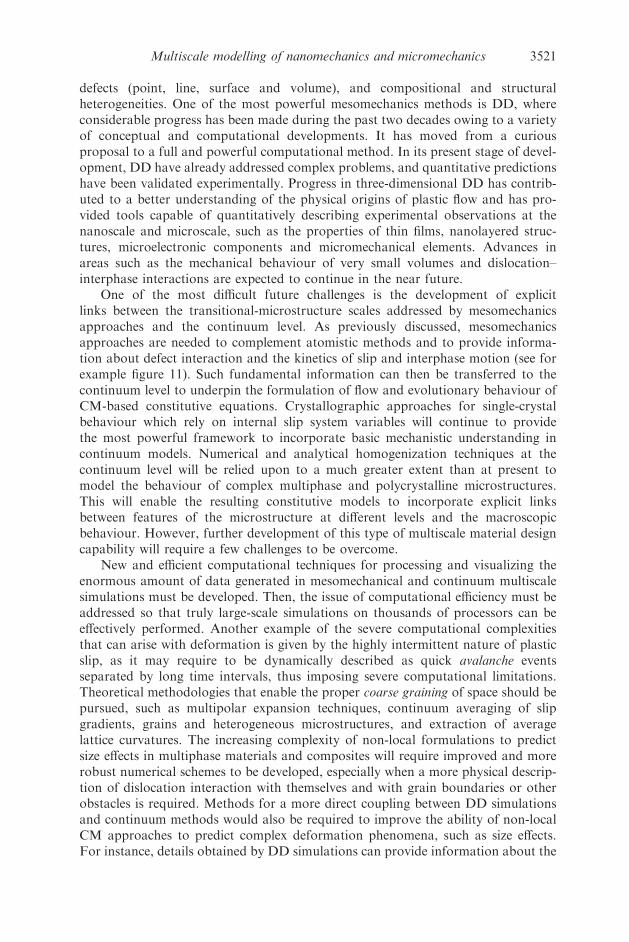
defects (point, line, surface and volume), and compositional and structuralheterogeneities. One of the most powerful mesomechanics methods is DD, whereconsiderable progress has been made during the past two decades owing to a varietyof conceptual and computational developments. It has moved from a curiousproposal to a full and powerful computational method. In its present stage of devel-opment, DD have already addressed complex problems, and quantitative predictionshave been validated experimentally. Progress in three-dimensional DD has contrib-uted to a better understanding of the physical origins of plastic flow and has pro-vided tools capable of quantitatively describing experimental observations at thenanoscale and microscale, such as the properties of thin films, nanolayered struc-tures, microelectronic components and micromechanical elements. Advances inareas such as the mechanical behaviour of very small volumes and dislocation–interphase interactions are expected to continue in the near future.

One of the most difficult future challenges is the development of explicitlinks between the transitional-microstructure scales addressed by mesomechanicsapproaches and the continuum level. As previously discussed, mesomechanicsapproaches are needed to complement atomistic methods and to provide informa-tion about defect interaction and the kinetics of slip and interphase motion (see forexample figure 11). Such fundamental information can then be transferred to thecontinuum level to underpin the formulation of flow and evolutionary behaviour ofCM-based constitutive equations. Crystallographic approaches for single-crystalbehaviour which rely on internal slip system variables will continue to providethe most powerful framework to incorporate basic mechanistic understanding incontinuum models. Numerical and analytical homogenization techniques at thecontinuum level will be relied upon to a much greater extent than at present tomodel the behaviour of complex multiphase and polycrystalline microstructures.This will enable the resulting constitutive models to incorporate explicit linksbetween features of the microstructure at different levels and the macroscopicbehaviour. However, further development of this type of multiscale material designcapability will require a few challenges to be overcome.

New and efficient computational techniques for processing and visualizing theenormous amount of data generated in mesomechanical and continuum multiscalesimulations must be developed. Then, the issue of computational efficiency must beaddressed so that truly large-scale simulations on thousands of processors can beeffectively performed. Another example of the severe computational complexitiesthat can arise with deformation is given by the highly intermittent nature of plasticslip, as it may require to be dynamically described as quick avalanche eventsseparated by long time intervals, thus imposing severe computational limitations.Theoretical methodologies that enable the proper coarse graining of space should bepursued, such as multipolar expansion techniques, continuum averaging of slipgradients, grains and heterogeneous microstructures, and extraction of averagelattice curvatures. The increasing complexity of non-local formulations to predictsize effects in multiphase materials and composites will require improved and morerobust numerical schemes to be developed, especially when a more physical descrip-tion of dislocation interaction with themselves and with grain boundaries or otherobstacles is required. Methods for a more direct coupling between DD simulationsand continuum methods would also be required to improve the ability of non-localCM approaches to predict complex deformation phenomena, such as size effects.For instance, details obtained by DD simulations can provide information about the


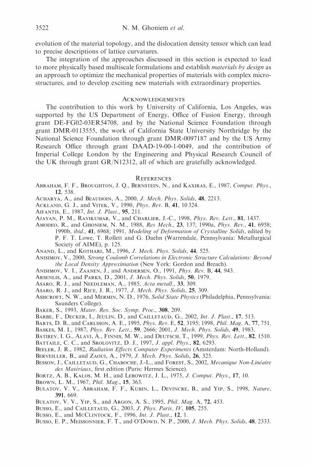
evolution of the material topology, and the dislocation density tensor which can leadto precise descriptions of lattice curvatures.

The integration of the approaches discussed in this section is expected to leadto more physically based multiscale formulations and establish materials by design asan approach to optimize the mechanical properties of materials with complex micro-structures, and to develop exciting new materials with extraordinary properties.

Acknowledgements

The contribution to this work by University of California, Los Angeles, wassupported by the US Department of Energy, Office of Fusion Energy, throughgrant DE-FG02-03ER54708, and by the National Science Foundation throughgrant DMR-0113555, the work of California State University Northridge by theNational Science Foundation through grant DMR-0097187 and by the US ArmyResearch Office through grant DAAD-19-00-1-0049, and the contribution ofImperial College London by the Engineering and Physical Research Council ofthe UK through grant GR/N12312, all of which are gratefully acknowledged.

References

Abraham, F. F., Broughton, J. Q., Bernstein, N., and Kaxiras, E., 1987, Comput. Phys.,12, 538.

Acharya, A., and Beaudoin, A., 2000, J. Mech. Phys. Solids, 48, 2213.Ackland, G. J., and Vitek, V., 1990, Phys. Rev. B, 41, 10 324.Aifantis, E., 1987, Int. J. Plast., 95, 211.Ajayan, P. M., Ravikumar, V., and Charlier, J.-C., 1998, Phys. Rev. Lett., 81, 1437.Amodeo, R., and Ghoniem, N. M., 1988, Res Mech., 23, 137; 1990a, Phys. Rev., 41, 6958;

1990b, ibid., 41, 6968; 1991, Modeling of Deformation of Crystalline Solids, edited byP. F. T. Lowe, T. Rollett and G. Daehn (Warrendale, Pennsylvania: MetallurgicalSociety of AIME), p. 125.

Anand, L., and Kothari, M., 1996, J. Mech. Phys. Solids, 44, 525.Anisimov, V., 2000, Strong Coulomb Correlations in Electronic Structure Calculations: Beyond

the Local Density Approximation (New York: Gordon and Breach).Anisimov, V. I., Zaanen, J., and Andersen, O., 1991, Phys. Rev. B, 44, 943.Arsenlis, A., and Parks, D., 2001, J. Mech. Phys. Solids, 50, 1979.Asaro, R. J., and Needleman, A., 1985, Acta metall., 33, 309.Asaro, R. J., and Rice, J. R., 1977, J. Mech. Phys. Solids, 25, 309.Ashcroft, N. W., and Mermin, N. D., 1976, Solid State Physics (Philadelphia, Pennsylvania:

Saunders College).Baker, S., 1993, Mater. Res. Soc. Symp. Proc., 308, 209.Barbe, F., Decker, I., Jeulin, D., and Cailletaud, G., 2002, Int. J. Plast., 17, 513.Barts, D. B., and Carlsson, A. E., 1995, Phys. Rev. E, 52, 3195; 1998, Phil. Mag. A, 77, 751.Baskes, M. I., 1987, Phys. Rev. Lett., 59, 2666; 2001, J. Mech. Phys. Solids, 49, 1983.Batirev, I. G., Alavi, A., Finnis, M. W., and Deutsch, T., 1999, Phys. Rev. Lett., 82, 1510.Battaile, C. C., and Srolovitz, D. J., 1997, J. appl. Phys., 82, 6293.Beeler, J. R., 1982, Radiation Effects Computer Experiments (Amsterdam: North-Holland).Berveiller, B., and Zaoui, A., 1979, J. Mech. Phys. Solids, 26, 325.Besson, J., Cailletaud, G., Chaboche, J.-L., and Forest, S., 2002,Mecanique Non-Lineaire

des Materiaux, first edition (Paris: Hermes Science).Bortz, A. B., Kalos, M. H., and Lebowitz, J. L., 1975, J. Comput. Phys., 17, 10.Brown, L. M., 1967, Phil. Mag., 15, 363.Bulatov, V. V., Abraham, F. F., Kubin, L., Devincre, B., and Yip, S., 1998, Nature,

391, 669.Bulatov, V. V., Yip, S., and Argon, A. S., 1995, Phil. Mag. A, 72, 453.Busso, E., and Cailletaud, G., 2003, J. Phys. Paris, IV, 105, 255.Busso, E., and McClintock, F., 1996, Int. J. Plast., 12, 1.Busso, E. P., Meissonnier, F. T., and O’Dowd, N. P., 2000, J. Mech. Phys. Solids, 48, 2333.


Cai, W., de Koning, M., Bulatov, V. V., and Yip, S., 2000, Phys. Rev. Lett., 85, 3213.Campbell, G., Foiles, S., Huang, H., Hughes, D., King, W., Lassila, D., Nikkel, D.,

Diaz de la Rubia, T., Shu, J. Y., and Smyshlyaev, V. P., 1998, Mater. Sci. Engng,A251, 1.

Canova, G., Brechet, Y., and Kubin, L. P., 1992, Modeling of Plastic Deformation and itsEngineering Applications, edited by S. I. Anderson, J. B. Bilde-Sorensen, N. Hansen,D. Juul Jensen, T. Leffers, H. Lilholt, T. Lorentzen, O. B. Pedersen, and B. Ralph(Risø, Roskilde: Risø National Laboratory).

Canova, G., Brechet, Y., Kubin, L. P., DeVincre, B., Pontikis, V., and Condat, M.,1993, Microstructures and Physical Properties, edited by J. Rabiet (Geneva: CH-Transtech).

Car, R., and Parrinello, M., 1985, Phys. Rev. Lett., 55, 2471.Chan, S.-P., Chen, G., Gong, X., and Liu, Z., 2001, Phys. Rev. Lett., 87, 205 502.Chang, J. P., Cai, W., Bulatov, V. V., and Yip, S., 2001, Mater. Sci. Engng, A309, 160.Chen, N. X., 1990, Phys. Rev. Lett., 64, 1193.Cleri, F., Wolf, D., Yip, S., and Phillpot, S. R., 1997, Acta mater., 45, 4993.Cohen, R. E., Mehl, M., and Papaconstantopoulos, D. A., 1994, Phys. Rev. B, 50, 14 694.Crisfield, M. A., 1997, Non-linear Finite Element Analysis of Solids and Structures, Vols 1

and 2, fourth edition (New York: Wiley).Cuitin‹ o, A. M., and Ortiz, M., 1992, Modelling Simulation Mater. Sci. Engng, 1, 225.Daw, M., and Baskes, M., 1983, Phys. Rev. Lett., 50, 1285; 1984, Phys. Rev. B, 29, 6443.Denteneer, P. J., and van Haeringen, W., 1985, J. Phys. C, 18, 4127.DeVincre, B., and Condat, M., 1992, Acta metall., 40, 2629.DeVincre, B., and Kubin, L. P., 1994, Modelling Simulation Mater. Sci. Engng, 2, 559.DeVincre, B., Pontikis, V., Brechet, Y., Canova, G., Condat, M., and Kubin, L. P.,

1992, Microscopic Simulations of Complex Hydrodynamic Phenomena, edited byM. Mareschal and B. L. Lolian (New York: Plenum), p. 413.

deWit, R., 1960, Solid. St. Phys., 10, 249.Doran, D. G., 1970, Radiat. Effects, 2, 249.Dreizler, R. M., and Gross, E. K. U., 1990, Density Functional Theory (Berlin: Springer).Duesbery, M. S., and Vitek, V., 1998, Acta mater., 46, 1481.Dumitrica, T., Belytscko, T., and Yakobson, B. I., 2003, J. chem. Phys., 118, 9485.Du« rr, M., Raschke, M. B., Pehlke, E., and Ho« fer, U., 2001, Phys. Rev. Lett., 86, 123.Dykstra, C. E., 1988, Ab initio Calculation of the Structure and Properties of Molecules

(Amsterdam: Elsevier).El-Azab, A., 2000, Phys. Rev. B, 61, 11956.Erb, U., Palumbo, G., Zugic, R., and Aust, K., 1996, Treatise on Materials Science and

Engineering (Pittsburgh, Pennsylvania: The Minerals, Metals and Materials ResearchSociety), p. 93.

Ercolessi, F., and Adams, J., 1994, Europhys. Lett., 26, 583.Ercolessi, F., Tosatti, E., and Parrinello, M., 1986, Phys. Rev. Lett., 57, 719.Esche, S. K., Kinzel, G. L., and Altan, T., 1997, Int. J. numer. Meth. Engng, 40, 4577.Eschrig, H., 1989, Optimized LCAO Method and the Electronic Structure of Extended

Systems (Berlin: Springer).Eshelby, J. D., 1957, Proc. R. Soc. A, 241, 376.Essmann, U., and Mughrabi, H., 1979, Phil. Mag. A, 40, 731.Finnis, M., and Sinclair, J., 1984, Phil. Mag. A, 50, 45.Fleck, N. A., and Hutchinson, J., 1997, Adv. appl. Mech., 33, 295; 2001, J. Mech. Phys.

Solids, 49, 2245.Forest, S., 1998, Acta mater., 46, 3265.Frauenheim, T., Porezag, D., Elstner, M., Jungnickel, G., Elsner, J., Haugk, M., and

Sieck, A., 1998, Mater. Res. Soc. Symp. Proc., 491, 91.Fulde, P., 1993, Electron Correlations in Molecules and Solids (Berlin: Springer).Galli, G., and Mauri, F., 1994, Phys. Rev. Lett., 73, 3471.Gao, H., and Huang, Y., 2003, Scripta metall., 48, 113.Gavazza, S., and Barnett, D., 1976, J. Mech. Phys. Solids, 24, 171.Gear, C., 1971, Numerical Initial Value Problems in Ordinary Differential Equations

(Englewood Cliffs, New Jersey: Prentice-Hall).


Georges, A., Kotliar, G., Krauth, W., and Rozenberg, M., 1996, Rev. mod. Phys., 68, 13.Ghoniem, N. M., 1992, Non-Linear Phenomena in Material Science II, edited by L. Kubin and

G. Martin (Dordrecht: Kluwer); 1999, J. Engng Mater. Technol., 121, 136.Ghoniem, N. M., and Amodeo, R. J., 1988a, Solid St. Phenomena, 3–4, 377; 1988b, Int J.

Engng Sci., 26, 653; 1990, Patterns, Defects and Material Instabilities, edited byD. Walgreaf and N. Ghoniem (Dordrecht: Kluwer), p. 303.

Ghoniem, N. M., Huang, J., and Wang, Z., 2001, Phil. Mag. Lett., 82, 55.Ghoniem, N. M., Matthews, J. R., and Amodeo, R. J., 1990, Res Mech., 29, 197.Ghoniem, N. M., and Sun, L. Z., 1999, Phys. Rev. B, 60, 128.Ghoniem, N. M., Tong, S., Huang, J., Singh, B., and Wen, M., 2002, J. nucl. Mater., 307–

311, 843.Ghoniem, N. M., Tong, S.-H., and Sun, L. Z., 2000, Phys. Rev., 61, 913.Ghosh, S., Nowak, Z., and Lee, K., 2002, Acta mater., 45, 2215.Gillan, M. J., 1989, J. Phys.: condens. Matter, 1, 689.Goedecker, S., 1999, Rev. of mod. Phys., 71, 1085.Golubov, S. I., Liu, X. L., Huang, H. C., andWoo, C. H., 2001, Comput. Phys. Commun.,

137, 312.Gregor, V., and Kratochvil, J., 1990, Res. Mech., 29, 197.Groma, I., 1997, Phys. Rev. B, 56, 5807.Groma, I., and Pawley, G. S., 1993, Phil. Mag. A, 67, 1459.Gross, E. K. U., Kreibich, T., Lein, M., and Petersilka, M., 1998, Electron Correlations

and Materials Properties, edited by N. K. A. Gonis and M. Ciftan (New York:Kluwer-Plenum), p. 393.

Guluoglu, A. N., Srolovitz, D. J., LeSar, R., and Lomdahl, R. S., 1989, Scripta metall.,23, 1347.

Gumbsch, P., and Gao, H., 1999, Science, 283, 965.Gunnarsson, O., and Lundqvist, B. I., 1976, Phys. Rev. B, 13, 4274.Gurtin, M. E., 2000, J. Mech. Phys. Solids, 48, 989; 2003, Int. J. Plast., 19, 47.Ha« hner, P., 1996, Appl. Phys. A, 62, 473.Ha« hner, P., Bay, K., and Zaiser, M., 1998, Phys. Rev. Lett., 81, 2470.Hamilton, J. C., 1997, Phys. Rev. B, 55, R7402.Hamilton, J. C., Stumpf, R., Bromann, K., Giovannini, M., Kern, K., and Brune, H.,

1999, Phys. Rev. Lett., 82, 4488.Harris, J., and Jones, R. O., 1974, J. Phys. F, 4, 1170.Hartley, C., 2003, Proceedings of the International Conference on Plasticity, Quebec City,

Canada. Phil. Mag., this issue.Hedin, L., and Lundqvist, S., 1969, Solid St. Phys., 23, 1; 1971, J. Phys. C, 4, 2064.Heinisch, H. L., 1995, Nucl. Instrum. Meth. B, 102, 47.Herve, E., and Zaoui, A., 1993, Int. J. Engng Sci., 31, 1.Hill, R., 1950, The Mathematical Theory of Plasticity, fourth edition (Oxford: Clarendon);

1965, J. Mech. Phys. Solids, 14, 89.Hirth, J. P., Rhee, M., and Zbib, H., 1996, J. Comput.-Aided Mater. Des., 3, 164.Hoagland, R. G., Hirth, J. P., and Gehlen, P. C., 1976, Phil. Mag. A, 34, 413.Hohenberg, P., and Kohn, W., 1964, Phys. Rev., 136, B864.Hoover, W. G., 1985, Phys. Rev. A, 31, 1695.Huang, H. C., Ghoniem, N. M., Diaz de la Rubia, T., Rhee, M., Zbib, H., and Hirth, J.

P., 1999, J. Engng Mater. Technol., 121, 143.Huang, H. C., Ghoniem, N. M., Wong, J. K., and Baskes, M. I., 1995,Modelling Simulation

Mater. Sci. Engng, 3, 615.Huber, N., and Tsakmakis, C., 1999, J. Mech. Phys. Solids, 47, 1589.Hughes, D., Chrzan, D., Liu, Q., and Hansen, N., 1998, Phys. Rev. Lett., 81, 4664.Ismail-Beigi, S., and Arias, T. A., 1999, Phys. Rev. Lett., 82, 2127.James, F., 1980, Rep. Prog. Phys., 43, 1145; 1990, Comput. Phys. Commun., 60, 329.Janotti, A., Zhang, S. B., Wei, S.-H. and van de Walle, C. G., 2002, Phys. Rev. Lett.,

89, 086 403.Jones, R. O., and Gunnarsson, O., 1989, Rev. mod. Phys., 61, 689.Jordan, E., and Walker, K., 1992, J. Engng Mater. Technol., 114, 19.


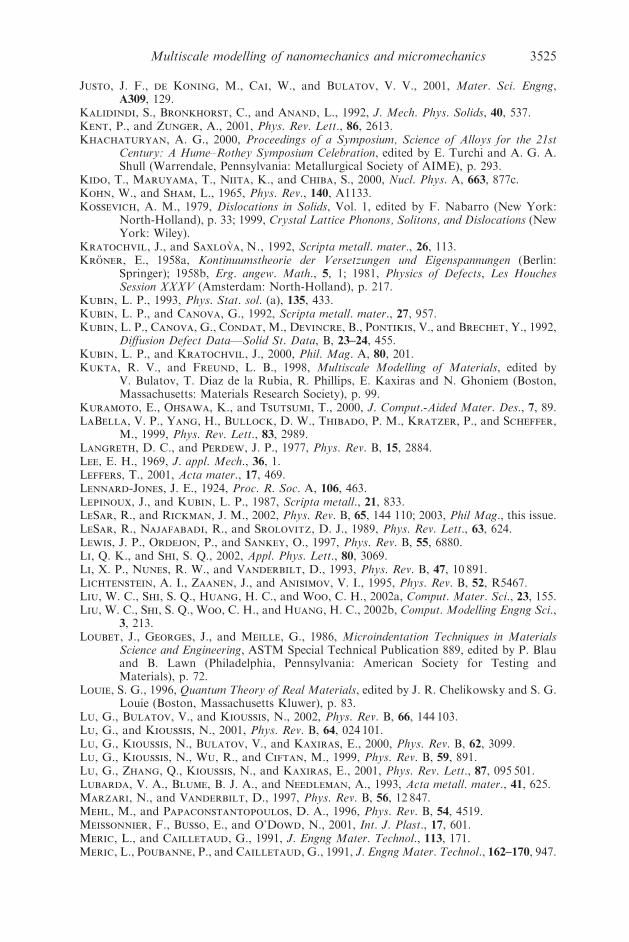
Justo, J. F., de Koning, M., Cai, W., and Bulatov, V. V., 2001, Mater. Sci. Engng,A309, 129.

Kalidindi, S., Bronkhorst, C., and Anand, L., 1992, J. Mech. Phys. Solids, 40, 537.Kent, P., and Zunger, A., 2001, Phys. Rev. Lett., 86, 2613.Khachaturyan, A. G., 2000, Proceedings of a Symposium, Science of Alloys for the 21st

Century: A Hume–Rothey Symposium Celebration, edited by E. Turchi and A. G. A.Shull (Warrendale, Pennsylvania: Metallurgical Society of AIME), p. 293.

Kido, T., Maruyama, T., Niita, K., and Chiba, S., 2000, Nucl. Phys. A, 663, 877c.Kohn, W., and Sham, L., 1965, Phys. Rev., 140, A1133.Kossevich, A. M., 1979, Dislocations in Solids, Vol. 1, edited by F. Nabarro (New York:

North-Holland), p. 33; 1999, Crystal Lattice Phonons, Solitons, and Dislocations (NewYork: Wiley).

Kratochvil, J., and Saxlov' a, N., 1992, Scripta metall. mater., 26, 113.Kro« ner, E., 1958a, Kontinuumstheorie der Versetzungen und Eigenspannungen (Berlin:

Springer); 1958b, Erg. angew. Math., 5, 1; 1981, Physics of Defects, Les HouchesSession XXXV (Amsterdam: North-Holland), p. 217.

Kubin, L. P., 1993, Phys. Stat. sol. (a), 135, 433.Kubin, L. P., and Canova, G., 1992, Scripta metall. mater., 27, 957.Kubin, L. P., Canova, G., Condat, M., Devincre, B., Pontikis, V., and Brechet, Y., 1992,

Diffusion Defect Data—Solid St. Data, B, 23–24, 455.Kubin, L. P., and Kratochvil, J., 2000, Phil. Mag. A, 80, 201.Kukta, R. V., and Freund, L. B., 1998, Multiscale Modelling of Materials, edited by

V. Bulatov, T. Diaz de la Rubia, R. Phillips, E. Kaxiras and N. Ghoniem (Boston,Massachusetts: Materials Research Society), p. 99.

Kuramoto, E., Ohsawa, K., and Tsutsumi, T., 2000, J. Comput.-Aided Mater. Des., 7, 89.LaBella, V. P., Yang, H., Bullock, D. W., Thibado, P. M., Kratzer, P., and Scheffer,

M., 1999, Phys. Rev. Lett., 83, 2989.Langreth, D. C., and Perdew, J. P., 1977, Phys. Rev. B, 15, 2884.Lee, E. H., 1969, J. appl. Mech., 36, 1.Leffers, T., 2001, Acta mater., 17, 469.Lennard-Jones, J. E., 1924, Proc. R. Soc. A, 106, 463.Lepinoux, J., and Kubin, L. P., 1987, Scripta metall., 21, 833.LeSar, R., and Rickman, J. M., 2002, Phys. Rev. B, 65, 144 110; 2003, Phil Mag., this issue.LeSar, R., Najafabadi, R., and Srolovitz, D. J., 1989, Phys. Rev. Lett., 63, 624.Lewis, J. P., Ordejon, P., and Sankey, O., 1997, Phys. Rev. B, 55, 6880.Li, Q. K., and Shi, S. Q., 2002, Appl. Phys. Lett., 80, 3069.Li, X. P., Nunes, R. W., and Vanderbilt, D., 1993, Phys. Rev. B, 47, 10 891.Lichtenstein, A. I., Zaanen, J., and Anisimov, V. I., 1995, Phys. Rev. B, 52, R5467.Liu, W. C., Shi, S. Q., Huang, H. C., and Woo, C. H., 2002a, Comput. Mater. Sci., 23, 155.Liu, W. C., Shi, S. Q., Woo, C. H., and Huang, H. C., 2002b, Comput. Modelling Engng Sci.,

3, 213.Loubet, J., Georges, J., and Meille, G., 1986, Microindentation Techniques in Materials

Science and Engineering, ASTM Special Technical Publication 889, edited by P. Blauand B. Lawn (Philadelphia, Pennsylvania: American Society for Testing andMaterials), p. 72.

Louie, S. G., 1996, Quantum Theory of Real Materials, edited by J. R. Chelikowsky and S. G.Louie (Boston, Massachusetts Kluwer), p. 83.

Lu, G., Bulatov, V., and Kioussis, N., 2002, Phys. Rev. B, 66, 144 103.Lu, G., and Kioussis, N., 2001, Phys. Rev. B, 64, 024 101.Lu, G., Kioussis, N., Bulatov, V., and Kaxiras, E., 2000, Phys. Rev. B, 62, 3099.Lu, G., Kioussis, N., Wu, R., and Ciftan, M., 1999, Phys. Rev. B, 59, 891.Lu, G., Zhang, Q., Kioussis, N., and Kaxiras, E., 2001, Phys. Rev. Lett., 87, 095 501.Lubarda, V. A., Blume, B. J. A., and Needleman, A., 1993, Acta metall. mater., 41, 625.Marzari, N., and Vanderbilt, D., 1997, Phys. Rev. B, 56, 12 847.Mehl, M., and Papaconstantopoulos, D. A., 1996, Phys. Rev. B, 54, 4519.Meissonnier, F., Busso, E., and O’Dowd, N., 2001, Int. J. Plast., 17, 601.Meric, L., and Cailletaud, G., 1991, J. Engng Mater. Technol., 113, 171.Meric, L., Poubanne, P., and Cailletaud, G., 1991, J. EngngMater. Technol., 162–170, 947.


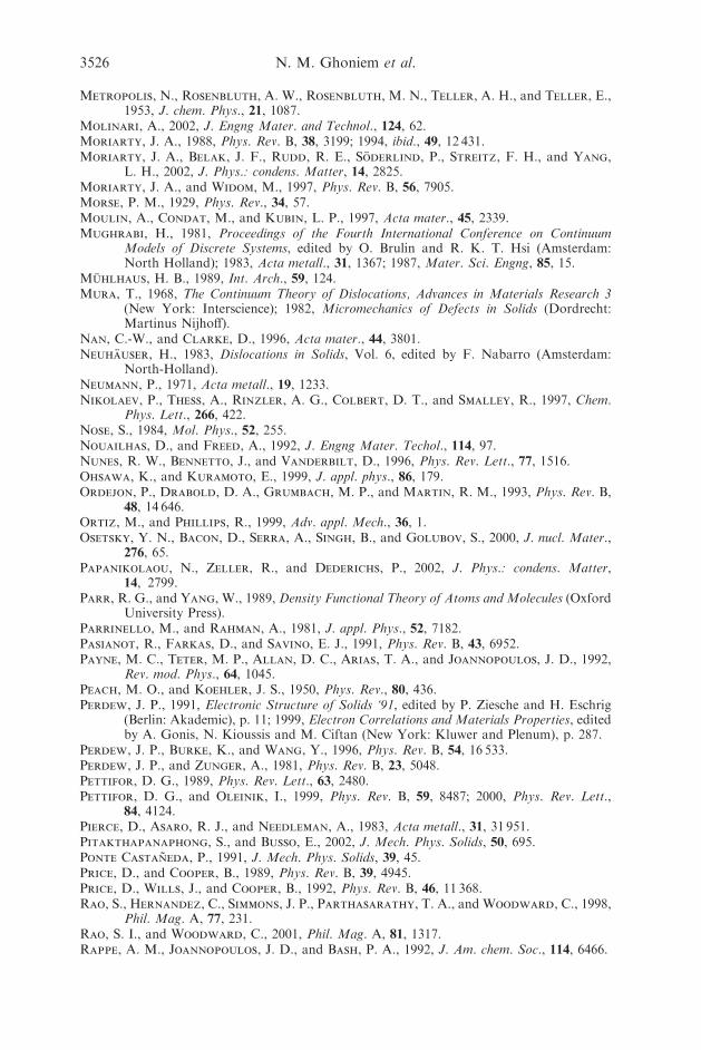
Metropolis, N., Rosenbluth, A. W., Rosenbluth, M. N., Teller, A. H., and Teller, E.,1953, J. chem. Phys., 21, 1087.

Molinari, A., 2002, J. Engng Mater. and Technol., 124, 62.Moriarty, J. A., 1988, Phys. Rev. B, 38, 3199; 1994, ibid., 49, 12 431.Moriarty, J. A., Belak, J. F., Rudd, R. E., So« derlind, P., Streitz, F. H., and Yang,

L. H., 2002, J. Phys.: condens. Matter, 14, 2825.Moriarty, J. A., and Widom, M., 1997, Phys. Rev. B, 56, 7905.Morse, P. M., 1929, Phys. Rev., 34, 57.Moulin, A., Condat, M., and Kubin, L. P., 1997, Acta mater., 45, 2339.Mughrabi, H., 1981, Proceedings of the Fourth International Conference on Continuum

Models of Discrete Systems, edited by O. Brulin and R. K. T. Hsi (Amsterdam:North Holland); 1983, Acta metall., 31, 1367; 1987, Mater. Sci. Engng, 85, 15.

Mu« hlhaus, H. B., 1989, Int. Arch., 59, 124.Mura, T., 1968, The Continuum Theory of Dislocations, Advances in Materials Research 3

(New York: Interscience); 1982, Micromechanics of Defects in Solids (Dordrecht:Martinus Nijhoff).

Nan, C.-W., and Clarke, D., 1996, Acta mater., 44, 3801.Neuha« user, H., 1983, Dislocations in Solids, Vol. 6, edited by F. Nabarro (Amsterdam:

North-Holland).Neumann, P., 1971, Acta metall., 19, 1233.Nikolaev, P., Thess, A., Rinzler, A. G., Colbert, D. T., and Smalley, R., 1997, Chem.

Phys. Lett., 266, 422.Nose, S., 1984, Mol. Phys., 52, 255.Nouailhas, D., and Freed, A., 1992, J. Engng Mater. Techol., 114, 97.Nunes, R. W., Bennetto, J., and Vanderbilt, D., 1996, Phys. Rev. Lett., 77, 1516.Ohsawa, K., and Kuramoto, E., 1999, J. appl. phys., 86, 179.Ordejon, P., Drabold, D. A., Grumbach, M. P., and Martin, R. M., 1993, Phys. Rev. B,

48, 14 646.Ortiz, M., and Phillips, R., 1999, Adv. appl. Mech., 36, 1.Osetsky, Y. N., Bacon, D., Serra, A., Singh, B., and Golubov, S., 2000, J. nucl. Mater.,

276, 65.Papanikolaou, N., Zeller, R., and Dederichs, P., 2002, J. Phys.: condens. Matter,

14, 2799.Parr, R. G., and Yang, W., 1989, Density Functional Theory of Atoms and Molecules (Oxford

University Press).Parrinello, M., and Rahman, A., 1981, J. appl. Phys., 52, 7182.Pasianot, R., Farkas, D., and Savino, E. J., 1991, Phys. Rev. B, 43, 6952.Payne, M. C., Teter, M. P., Allan, D. C., Arias, T. A., and Joannopoulos, J. D., 1992,

Rev. mod. Phys., 64, 1045.Peach, M. O., and Koehler, J. S., 1950, Phys. Rev., 80, 436.Perdew, J. P., 1991, Electronic Structure of Solids ‘91, edited by P. Ziesche and H. Eschrig

(Berlin: Akademic), p. 11; 1999, Electron Correlations and Materials Properties, editedby A. Gonis, N. Kioussis and M. Ciftan (New York: Kluwer and Plenum), p. 287.

Perdew, J. P., Burke, K., and Wang, Y., 1996, Phys. Rev. B, 54, 16 533.Perdew, J. P., and Zunger, A., 1981, Phys. Rev. B, 23, 5048.Pettifor, D. G., 1989, Phys. Rev. Lett., 63, 2480.Pettifor, D. G., and Oleinik, I., 1999, Phys. Rev. B, 59, 8487; 2000, Phys. Rev. Lett.,

84, 4124.Pierce, D., Asaro, R. J., and Needleman, A., 1983, Acta metall., 31, 31 951.Pitakthapanaphong, S., and Busso, E., 2002, J. Mech. Phys. Solids, 50, 695.Ponte Castan‹ eda, P., 1991, J. Mech. Phys. Solids, 39, 45.Price, D., and Cooper, B., 1989, Phys. Rev. B, 39, 4945.Price, D., Wills, J., and Cooper, B., 1992, Phys. Rev. B, 46, 11 368.Rao, S., Hernandez, C., Simmons, J. P., Parthasarathy, T. A., and Woodward, C., 1998,

Phil. Mag. A, 77, 231.Rao, S. I., and Woodward, C., 2001, Phil. Mag. A, 81, 1317.Rappe, A. M., Joannopoulos, J. D., and Bash, P. A., 1992, J. Am. chem. Soc., 114, 6466.


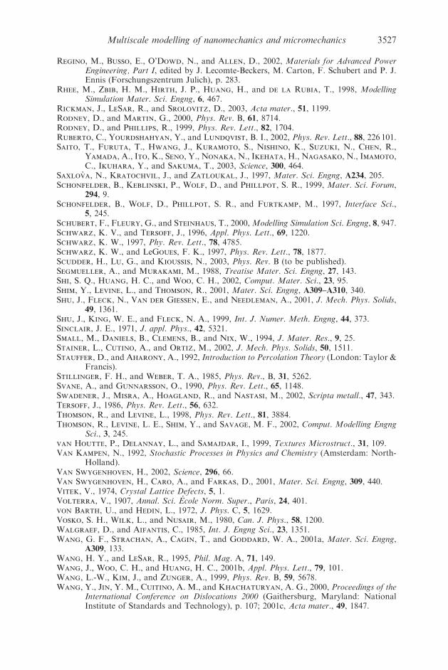
Regino, M., Busso, E., O’Dowd, N., and Allen, D., 2002, Materials for Advanced PowerEngineering, Part I, edited by J. Lecomte-Beckers, M. Carton, F. Schubert and P. J.Ennis (Forschungszentrum Julich), p. 283.

Rhee, M., Zbib, H. M., Hirth, J. P., Huang, H., and de la Rubia, T., 1998, ModellingSimulation Mater. Sci. Engng, 6, 467.

Rickman, J., LeSar, R., and Srolovitz, D., 2003, Acta mater., 51, 1199.Rodney, D., and Martin, G., 2000, Phys. Rev. B, 61, 8714.Rodney, D., and Phillips, R., 1999, Phys. Rev. Lett., 82, 1704.Ruberto, C., Yourdshahyan, Y., and Lundqvist, B. I., 2002, Phys. Rev. Lett., 88, 226 101.Saito, T., Furuta, T., Hwang, J., Kuramoto, S., Nishino, K., Suzuki, N., Chen, R.,

Yamada, A., Ito, K., Seno, Y., Nonaka, N., Ikehata, H., Nagasako, N., Imamoto,C., Ikuhara, Y., and Sakuma, T., 2003, Science, 300, 464.

Saxlov' a, N., Kratochvil, J., and Zatloukal, J., 1997, Mater. Sci. Engng, A234, 205.Schonfelder, B., Keblinski, P., Wolf, D., and Phillpot, S. R., 1999, Mater. Sci. Forum,

294, 9.Schonfelder, B., Wolf, D., Phillpot, S. R., and Furtkamp, M., 1997, Interface Sci.,

5, 245.Schubert, F., Fleury, G., and Steinhaus, T., 2000,Modelling Simulation Sci. Engng, 8, 947.Schwarz, K. V., and Tersoff, J., 1996, Appl. Phys. Lett., 69, 1220.Schwarz, K. W., 1997, Phy. Rev. Lett., 78, 4785.Schwarz, K. W., and LeGoues, F. K., 1997, Phys. Rev. Lett., 78, 1877.Scudder, H., Lu, G., and Kioussis, N., 2003, Phys. Rev. B (to be published).Segmueller, A., and Murakami, M., 1988, Treatise Mater. Sci. Engng, 27, 143.Shi, S. Q., Huang, H. C., and Woo, C. H., 2002, Comput. Mater. Sci., 23, 95.Shim, Y., Levine, L., and Thomson, R., 2001, Mater. Sci. Engng, A309–A310, 340.Shu, J., Fleck, N., Van der Giessen, E., and Needleman, A., 2001, J. Mech. Phys. Solids,

49, 1361.Shu, J., King, W. E., and Fleck, N. A., 1999, Int. J. Numer. Meth. Engng, 44, 373.Sinclair, J. E., 1971, J. appl. Phys., 42, 5321.Small, M., Daniels, B., Clemens, B., and Nix, W., 1994, J. Mater. Res., 9, 25.Stainer, L., Cutino, A., and Ortiz, M., 2002, J. Mech. Phys. Solids, 50, 1511.Stauffer, D., and Aharony, A., 1992, Introduction to Percolation Theory (London: Taylor &

Francis).Stillinger, F. H., and Weber, T. A., 1985, Phys. Rev., B, 31, 5262.Svane, A., and Gunnarsson, O., 1990, Phys. Rev. Lett., 65, 1148.Swadener, J., Misra, A., Hoagland, R., and Nastasi, M., 2002, Scripta metall., 47, 343.Tersoff, J., 1986, Phys. Rev. Lett., 56, 632.Thomson, R., and Levine, L., 1998, Phys. Rev. Lett., 81, 3884.Thomson, R., Levine, L. E., Shim, Y., and Savage, M. F., 2002, Comput. Modelling Engng

Sci., 3, 245.van Houtte, P., Delannay, L., and Samajdar, I., 1999, Textures Microstruct., 31, 109.Van Kampen, N., 1992, Stochastic Processes in Physics and Chemistry (Amsterdam: North-

Holland).Van Swygenhoven, H., 2002, Science, 296, 66.Van Swygenhoven, H., Caro, A., and Farkas, D., 2001, Mater. Sci. Engng, 309, 440.Vitek, V., 1974, Crystal Lattice Defects, 5, 1.Volterra, V., 1907, Annal. Sci. Ecole Norm. Super., Paris, 24, 401.von Barth, U., and Hedin, L., 1972, J. Phys. C, 5, 1629.Vosko, S. H., Wilk, L., and Nusair, M., 1980, Can. J. Phys., 58, 1200.Walgraef, D., and Aifantis, C., 1985, Int. J. Engng Sci., 23, 1351.Wang, G. F., Strachan, A., Cagin, T., and Goddard, W. A., 2001a, Mater. Sci. Engng,

A309, 133.Wang, H. Y., and LeSar, R., 1995, Phil. Mag. A, 71, 149.Wang, J., Woo, C. H., and Huang, H. C., 2001b, Appl. Phys. Lett., 79, 101.Wang, L.-W., Kim, J., and Zunger, A., 1999, Phys. Rev. B, 59, 5678.Wang, Y., Jin, Y. M., Cuitino, A. M., and Khachaturyan, A. G., 2000, Proceedings of the

International Conference on Dislocations 2000 (Gaithersburg, Maryland: NationalInstitute of Standards and Technology), p. 107; 2001c, Acta mater., 49, 1847.


Wang, Z., Ghoniem, N., LeSar, R., and Sriram, S., 2003a, Modelling Simulation Mater.Sci. Engng (submitted).

Wang, Z., LeSar, R., and Ghoniem, N., 2003b (to be published).Wimmer, E., Krakauer, H., Weinert, M., and Freeman, A., 1981, Phys. Rev. B, 24, 864.Woo, C. H., Huang, H. C., and Zhu, W. J., 2002, Appl. Phys. A, 76, 101.Woo, C. H., and Puls, M. P., 1976, J. Phys. C, 9, L27.Woodward, C., and Rao, S. I., 2002, Phys. Rev. Lett., 88, 216 402.Wu, R., Freeman, A., and Olson, G., 1994, Science, 265, 376.Wu, T., Lee, C.-K., and Wang, R., 1993, Mater. Res. Soc. Symp. Proc., 308, 133.Xu, W., and Moriarty, J. A., 1996, Phys. Rev. B, 54, 6941; 1998, Comput. Mater. Sci., 9, 348.Yang, W., 1991, Phys. Rev. Lett., 66, 1438.Yildirim, T., Gu« lseren, O., and Ciraci, S., 2001, Phys. Rev., B, 64, 075 404.Zaiser, M., 2001, Mater. Science Engng, A309–A310, 304.Zaiser, M., Avlonitis, M., and Aifantis, E. C., 1998, Acta mater., 46, 4143.Zaiser, M., and Ha« hner, P., 1997, Phys. Stat. sol. (b), 199, 267.Zbib, H., and Aifantis, E., 1988, Res. Mech., 23, 261.Zbib, R. M., Rhee, M., and Hirth, J. P., 1998, Int. J. Mech. Sci., 40, 113.Zhang, W. Q., Xie, Q., Ge, X. J., and Chen, N. X., 1997, J. appl. Phys., 82, 578.Zhou, S. J., Preston, D. L., Lomdahl, P. S., and Beazley, D. M., 1998, Science, 279, 1525.Zienkiewicz, O. C., and Taylor, R. L., 1994, The Finite Element Method, fourth edition

(New York: McGraw-Hill).

3528 Multiscale modelling of nanomechanics and micromechanics

Documents

Multiscale modelling of nanomechanics and …nkioussi/publications/2003PhilMag.Review.pdfMultiscale modelling of nanomechanics and micromechanics: an overview ... (MMM) approaches