Multiscale Denoising of Photographic Images

Umesh Rajashekar and Eero P. Simoncelli

New York University

Chapter 11 in The Essential Guide to Image Processing, 2nd edition, pages:241-261.

Editor: Al Bovik, Academic Press, 2009

1 Introduction

Signal acquisition is a noisy business. In photographic images, there is noise within the light intensity signal(e.g., photon noise), and additional noise can arise within the sensor (e.g., thermal noise in a CMOS chip),as well as in subsequent processing (e.g., quantization). Image noise can be quite noticeable, as in imagescaptured by inexpensive cameras built into cellular telephones, or imperceptible, as in images captured byprofessional digital cameras. Stated simply, the goal of image denoising is to recover the “true” signal (or itsbest approximation) from these noisy acquired observations. All such methods rely on understanding andexploiting the differences between the properties of signal and noise.

Formally, solutions to the denoising problem rely on three fundamental components: a signal model,a noise model, and finally a measure of signal fidelity (commonly known as the objective function) thatis to be minimized. In this chapter, we’ll describe the basics of image denoising, with an emphasis onsignal properties. For noise modeling, we’ll restrict ourselves to the case in which images are corrupted byadditive, white, Gaussian noise - that is, we’ll assume each pixel is contaminated by adding a sample drawnindependently from a Gaussian probability distribution of fixed variance. A variety of other noise modelsand corruption processes are considered in Chapter 7. Throughout, we’ll use the well known mean squarederror (MSE) measure as an objective function.

We develop a sequence of three image denoising methods, motivating each one by observing a particularproperty of photographic images that emerges when they are decomposed into subbands at different spatialscales. We’ll examine each of these properties quantitatively by examining statistics across a training set ofphotographic images and noise samples. And for each property, we’ll use this quantitative characterization todevelop two example denoising functions: a binary threshold function that retains or discards each multi-scalecoefficient depending on whether it is more likely to be dominated by noise or signal, and a continuous-valuedfunction that multiplies each coefficient by an optimized scalar value. Although these methods are quitesimple, they capture many of the concepts that are used in state-of-the-art denoising systems. Toward theend of the chapter, we briefly describe several alternative approaches.

2 Distinguishing Images from Noise in Multiscale Representations

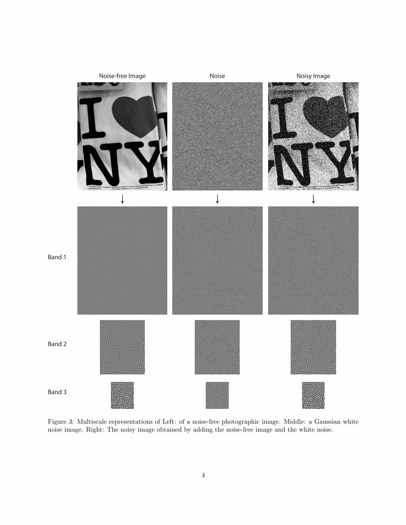
Consider the images in the top row of Figure 3. Your visual system is able to recognize effortlessly thatthe image in the left column is a photograph while the image in the middle column is filled with noise.How does it do this? We might hypothesize that it simply recognizes the difference in the distributionsof pixel values in the two images. But the distribution of pixel values of photographic images is highlyinconsistent from image to image, and more importantly, one can easily generate a noise image whose pixeldistribution is matched to any given image (by simply spatially scrambling the pixels). So it seems thatvisual discrimination of photographs and noise cannot be accomplished based on the statistics of individual

1

256

Fourier

Transform

256

Band-0

(Residual)

256

Band-1

128

Band-2

64

Low Pass

Band

256

Figure 1: A graphical depiction of the multiscale image representation used for all examples in this chapter.Left column: An image and its centered Fourier transform. The white circles represent filters used to selectbands of spatial frequencies. Middle column: Inverse Fourier transforms of the various spatial frequenciesbands selected by the idealized filters in the left column. Each filtered image represents only a subset ofthe entire frequency space (indicated by the arrows originating from the left column). Depending on theirmaximum spatial frequency, some of these filtered images can be downsampled in the pixel domain withoutany loss of information. Right column: Downsampled versions of the filtered images in the middle column.The resulting images form the subbands of a multiscale “pyramid” representation [1,2]. The original imagecan be exactly recovered from these subbands by reversing the procedure used to construct the representation.

2

Noisy Image Denoised Image

y x(y) x

Figure 2: Block diagram of multiscale denoising. The noisy photographic image is first decomposed into amultiscale representation. The noisy pyramid coefficients, y, are then denoised using the functions, x(y),resulting in denoised coefficients, x. Finally, the pyramid of denoised coefficients used to reconstruct thedenoised image.

pixels. Nevertheless, the joint statistics of pixels reveal striking differences, and these may be exploited todistinguish photographs from noise, and also to restore an image that has been corrupted by noise, a processcommonly referred to as denoising. Perhaps the most obvious (and historically, the oldest) observationis that spatially proximal pixels of photographs are correlated, whereas the noise pixels are not. Thus, asimple strategy for denoising an image is to separate it into smooth and non-smooth parts, or equivalently,low-frequency and a high-frequency components. This decomposition can then be applied recursively to thelowpass component to generate a multi-scale representation, as illustrated in Figure 1. The lower frequencysubbands are smoother, and thus can be subsampled to allow a more efficient representation, generallyknown as a multiscale pyramid [1,2]. The resulting collection of frequency subbands contains the exact sameinformation as the input image, but, as we shall see, it has been separated in such a way that it is more easilydistinguished from noise. A detailed development of multiscale representations can be found in Chapter 6of this book.

Transformation of an input image to a multiscale image representation has almost become a de facto pre-processing step for a wide variety of image processing and computer vision applications. For this chapter,we’ll assume a three-step denoising methodology:

1. Compute the multiscale representation of the noisy image.

2. Denoise the noisy coefficients, y, of all bands except the low pass band using denoising functions x(y)to get an estimate, x, of the true signal coefficient, x.

3. Invert the multiscale representation (i.e., recombine the subbands) to obtain a denoised image.

This sequence is illustrated in Figure 2. Given this general framework, our problem is to determine the formof the denoising functions, x(y).

3 Subband Denoising - A Global Approach

We begin by making some observations about the differences between photographic images and randomnoise. Figure 3 shows the multiscale decomposition of an essentially noise-free photograph, random noise,and a noisy image obtained by adding the two. The pixels of the signal (the noise-free photograph) lie in theinterval [0, 255]. The noise pixels are uncorrelated samples of a Gaussian distribution with zero mean andstandard deviation of 60. When we look at the subbands of the noisy image, we notice that band 1 of the

3

Noise-free Image

Band 3

Band 2

Band 1

Noise Noisy Image

Figure 3: Multiscale representations of Left: of a noise-free photographic image. Middle: a Gaussian whitenoise image. Right: The noisy image obtained by adding the noise-free image and the white noise.

4

0 1 2 3 4 5−8

−4

0

4

8

Log2 (variance)

0 1 2 3 4 5

0

0.5

1

Band Number

f( )

(A)

(B)

Figure 4: Band denoising functions. (A) Plot of average log variance of subbands of a multiscale pyramid asa function of the band number averaged over the photographic images in our training set (solid line, denotinglog(|~x|2)) and Gaussian white noise image of standard deviation of 60 (dashed line, denoting log(|~n|2). Forvisualization purposes, the curves have been normalized so that the log of the noise variance was equal to0.0 (B) Optimal thresholding function (black) and weighting function (gray) as a function of band number.

noisy image is almost indistinguishable from the corresponding band for the noise image; band 2 of the noisyimage is contaminated by noise, but some of the features from the original image remain visible; and band 3looks nearly identical to the corresponding band of the original image. These observations suggest that, onaverage, noise coefficients tend to have larger amplitude than signal coefficients in the high frequency bands(e.g. band 1), whereas signal coefficients tend to be more dominant in the low frequency bands (e.g. band3).

3.1 Band Thresholding

This observation about the relative strength of signal and noise in different frequency bands leads us to ourfirst denoising technique: we can set each coefficient that lies in a band that is significantly corrupted bynoise (e.g., band 1) to zero, and retain the other bands without modification. In other words, we make abinary decision to retain or discard each subband. But how do we decide which bands to keep and whichto discard? To address this issue, let us denote the entire band of noise-free image coefficients as a vector,~x, the coefficients of the noise image as ~n, and the band of noisy coefficients as ~y = ~x + ~n. Then the totalsquared error incurred if we should decide to retain the noisy band is |~x− ~y|2 = |~n|2, and the error incurredif we discard the band is |~x−~0|2 = |~x|2. Since our objective is to minimize the mean squared error betweenthe original and denoised coefficients, the optimal decision is to retain the band whenever the signal energy(i.e., the squared norm of the signal vector, ~x) is greater than that of the noise (i.e., |~x|2 > |~n|2) and discardit otherwise1

To implement this algorithm, we need to know the energy (or variance) of the noise-free signal, |~x|2, andnoise, |~n|2. There are several possible ways for us to obtain these.

• Method I : we can assume values for either or both, based on some prior knowledge or principles aboutimages or our measurement device.

• Method II : we can estimate them in advance from a set of “training” or calibration measurements.For the noise, we might imagine measuring the variability in the pixel values for photographs of a set

1Minimizing the total energy is equivalent to minimizing the mean squared error, since the latter is obtained from the former

by dividing by the number of elements.

5

of known test images. For the photographic images, we could measure the variance of subbands ofnoise-free images. In both cases, we must assume that our training images have the same varianceproperties as the images that we will subsequently denoise.

• Method III : we can attempt to determine the variance of signal and/or noise from the observed noisycoefficients of the image we are trying to denoise. For example, if the noise energy is known to have avalue of E2

n, we could estimate the signal energy as |~x|2 = |~y−~n|2 ≈ |~y|2−E2n, where the approximation

assumes that the noise is independent of the signal, and that the actual noise energy is close to theassumed value: |~n|2 ≈ E2

n.

These three methods of obtaining parameters may be combined, obtaining some parameters with one methodand others with another.

For our purposes, we assume that the noise variance is known in advance (Method I), and we use MethodII to obtain estimates of the signal variance by looking at values across a training set of images. Figure4A shows a plot of the variance as a function of the band number, for 30 photographic images2 (solid line)compared with that of 30 equal-sized Gaussian white noise images (dashed line) of a fixed standard deviationof 60. For ease of comparison, we have plotted the logarithm of the band variance, and normalized the curvesso that the variance of the noise bands is 1.0 (and hence the log variance is zero). The plot confirms ourobservation that, on average, noise dominates the higher frequency bands (0 through 2) and signal dominatesthe lower frequency bands (3 and above). Furthermore, we see that the signal variance is nearly a straightline. Figure 4B shows the optimal binary denoising function (solid black line) that results from assumingthese signal variances. This is a step function, with the step located at the point where the signal variancecrosses the noise variance.

We can examine the behavior of this method visually, by retaining or discarding the subbands of thepyramid of noisy coefficients according to the optimal rule in Figure 4B, and then generating a denoised imageby inverting the pyramid transformation. Figure 8C shows the result of applying this denoising technique tothe noisy image shown in Fig. 8B. We can see that a substantial amount of the noise has been eliminated,although the denoised image appears somewhat blurred since the high frequency bands have been discarded.The performance of this denoising scheme can be quantified using the mean squared error (MSE), or with therelated measure of peak signal-to-noise-ratio (PSNR), which is essentially a log-domain version of the mean

squared error. If we define the MSE between two vectors ~x and ~y, each of size N , as MSE(~x, ~y) = 1N|~x − ~y|

2,

then the PSNR (assuming 8-bit images) is defined as PSNR(~x, ~y) = 10 log102552

MSE(~x,~y) and measured in units

of decibels (dB). For the current example, the PSNR of the noisy and denoised image were 13.40dB and24.45dB respectively. Figure 9 shows the improvement in PSNR over the noisy image across 5 differentimages.

3.2 Band Weighting

In the previous section, we developed a binary denoising function based on knowledge of the relative strengthof signal and noise in each band. In general, we can write the solution for each individual coefficient:

x(~y) = f(|~y|) · y (1)

where the binary-valued function, f(·), is written as a function of the energy of the noisy coefficients, |~y|,to allow estimation of signal or noise variance from the observation (as described in Method III above).An examination of the pyramid decomposition of the noisy image in Figure 3 suggests that the binaryassumption is overly restrictive. Band 1, for example, contains some residual signal that is visible despitethe large amount of noise. And band 3 shows some noise in the presence of strong signal coefficients. Thisobservation suggests that instead of the binary retain-or-discard technique, we might obtain better resultsby allowing f(·) to take on real values that depend on the relative strength of the signal and noise.

2All images in our training set are of New York City street scenes, each of size 1536×1024 pixels. The images were acquired

using a Canon 30D digital SLR camera.

6

But how do we determine the optimal real-valued denoising function f(·)? For each band of noisycoefficients ~y, we seek a scalar value, a, that minimizes the error |a~y − ~x|2. To find the optimal value, wecan expand the error as a2~yT ~y − 2a~yT ~x + ~xT ~x, differentiate it with respect to a, set the result to zero, andsolve for a. The optimal value is found to be

a =~yT ~x

~yT ~y(2)

Using the fact that the noise is uncorrelated with the signal (i.e. ~xT~n ≈ 0) and the definition of the noisyimage ~y = ~x + ~n, we may express the optimal value as

a =|~x|2

|~x|2 + |~n|2(3)

That is, the optimal scalar multiplier is a value in the range [0, 1], which depends on the relative strength ofsignal and noise. As described under Method II in the previous section, we may estimate this quantity fromtraining examples.

To compute this function f(·), we performed a five-band decomposition of the images and noise in ourtraining set and computed the average values of |~x|2 and |~n|2, indicated by the solid and dashed lines inFigure 4A. The resulting function is plotted in gray as a function of the band number in Figure 4B. Asexpected, bands 0-1, which are dominated by noise, have a weight close to zero; bands 4 and above, whichhave more signal energy, have a weight close to 1.0; and bands 2-3 are weighted by intermediate values. Sincethis denoising function includes the binary functions as a special case, the denoising performance cannot beany worse than band thresholding, and will in general be better. To denoise a noisy image, we compute itsfive-band decomposition, and weight each band in accordance to its weight indicated in Figure 4B and invertthe pyramid to obtain the denoised image. An example of this denoising is shown in Figure 8D. The PSNRof the noisy and denoised images were 13.40dB and 25.04dB - an improvement of more than 11.5dB! Thisdenoising performance is consistent across images, as shown in Figure 9.

Previously, the value of the optimal scalar was derived using Method II. But we can use the fact that~x = ~y − ~n, and the knowledge that noise is uncorrelated with the signal (i.e. ~xT~n ≈ 0), to rewrite Eq. (2) asa function of each band as:

a = f(|~y|) =|~y|2 − |~n|2

|~y|2. (4)

If we assume that the noise energy is known, then this formulation is an example of Method III, and moregenerally, we now can rewrite x(~y) = f(|~y|) · y.

The denoising function in Eq. (4) is often applied to coefficients in a Fourier transform representation,where it is known as the ‘Wiener filter’. In this case, each Fourier transform coefficient is multiplied by avalue that depends on the variances of the signal and noise at each spatial frequency- that is, the powerspectra of the signal and noise. The power spectrum of natural images is commonly modeled using a powerlaw, F (Ω) = A/Ωp, where Ω is spatial frequency, p is the exponent controlling the falloff of the signal powerspectrum (typically near 2), A is a scale factor controlling the overall signal power, is the unique form that isconsistent with a process that is both translation- and scale-invariant (see Chapter 9). Note that this modelis consistent with the measurements of Figure 4, since the frequency of the subbands grows exponentiallywith the band number. If, in addition, the noise spectrum is assumed to be flat (as it would be, for example,with Gaussian white noise), then the Wiener filter is simply

|H(Ω)|2 =|A/Ωp|

|A/Ωp| + σ2N

, (5)

where σ2N is the noise variance.

7

Figure 5: Log histograms of coefficients of a band in the multiscale pyramid for a photographic image (solid)and Gaussian white noise of standard deviation of 60 (dashed). As expected, the log of the distribution ofthe Gaussian noise is parabolic.

4 Subband Coefficient Denoising - A Pointwise Approach

The general form of denoising in the Section 3 involved weighting the entire band by a single number -0 or 1 for band thresholding, or a scalar between 0 and 1 for band weighting. However, we can observethat in a noisy band such as band 2 in Figure 3, the amplitudes of signal coefficients tend to be either verysmall, or quite substantial. The simple interpretation is that images have isolated features such as edges thattend to produce large coefficients in a multiscale representation. The noise, on the other hand, is relativelyhomogeneous.

To verify this observation, we used the 30 images in our training set and 30 Gaussian white noise images(standard deviation of 60) of the same size and computed the distribution of signal and noise coefficients in aband. Figure 5 shows the log of the distribution of the magnitude of signal (solid line) and noise coefficients(dashed line) in one band of the multiscale decomposition. We can see that the distribution tails are heavierand the frequency of small values is higher for the signal coefficients, in agreement with our observationsabove.

From this basic observation, we can see that signal and noise coefficients might be further distinguishedbased on their magnitudes. This idea has been used for decades in video cassette recorders for removingmagnetic tape noise, where it is known as ”coring”. We capture it using a denoising function of the form:

x(y) = f(|y|) · y (6)

where x(y) is the estimate of a single noisy coefficient y. Note that unlike the denoising scheme in Eq. (1),the value of the denoising function, f(·), will now be different for each coefficient.

4.1 Coefficient-Thresholding

Consider first the case where the function f(·) is constrained to be binary, analogous to our previous devel-opment of band thresholding. Given a band of noisy coefficients, our goal now is to determine a thresholdsuch that coefficients whose magnitudes are less than this threshold are set to zero, and all coefficients whosemagnitudes are greater than or equal to the threshold are retained.

The criterion for selecting the threshold is again selected so as to minimize the mean squared error. Wedetermined this threshold empirically using our image training set. We computed the five-band pyramidfor the noise-free and noisy images (corrupted by Gaussian noise of standard deviation of 60) to get pairsof noisy coefficients, y, and their corresponding noise-free coefficients, x, for a particular band. Let us nowconsider an arbitrary threshold value, say T . As in the case of band thresholding, there are two types oferror introduced at any threshold level. First, when the magnitude of the observed coefficient, y, is below

8

0 100 200

0

100

200

0 300 6000

300

600

0 1000 20000

1000

2000

0 100 200

0

0.5

1

0 300 600

0

0.5

1

0 1000 2000

0

0.5

1

(A)

(B)

Band 1 Band 3Band 2

y

f(|y|)

x(y)

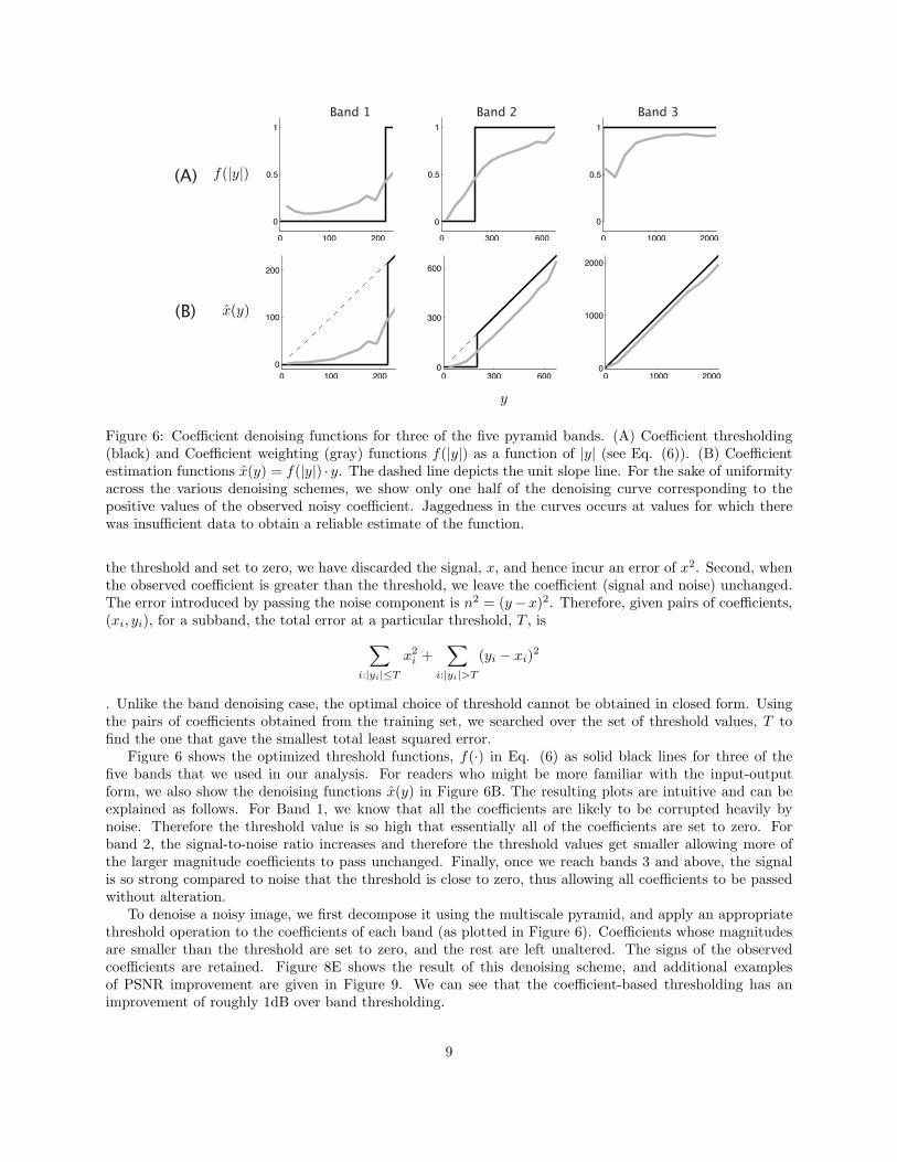
Figure 6: Coefficient denoising functions for three of the five pyramid bands. (A) Coefficient thresholding(black) and Coefficient weighting (gray) functions f(|y|) as a function of |y| (see Eq. (6)). (B) Coefficientestimation functions x(y) = f(|y|) · y. The dashed line depicts the unit slope line. For the sake of uniformityacross the various denoising schemes, we show only one half of the denoising curve corresponding to thepositive values of the observed noisy coefficient. Jaggedness in the curves occurs at values for which therewas insufficient data to obtain a reliable estimate of the function.

the threshold and set to zero, we have discarded the signal, x, and hence incur an error of x2. Second, whenthe observed coefficient is greater than the threshold, we leave the coefficient (signal and noise) unchanged.The error introduced by passing the noise component is n2 = (y−x)2. Therefore, given pairs of coefficients,(xi, yi), for a subband, the total error at a particular threshold, T , is

∑

i:|yi|≤T

x2i +

∑

i:|yi|>T

(yi − xi)2

. Unlike the band denoising case, the optimal choice of threshold cannot be obtained in closed form. Usingthe pairs of coefficients obtained from the training set, we searched over the set of threshold values, T tofind the one that gave the smallest total least squared error.

Figure 6 shows the optimized threshold functions, f(·) in Eq. (6) as solid black lines for three of thefive bands that we used in our analysis. For readers who might be more familiar with the input-outputform, we also show the denoising functions x(y) in Figure 6B. The resulting plots are intuitive and can beexplained as follows. For Band 1, we know that all the coefficients are likely to be corrupted heavily bynoise. Therefore the threshold value is so high that essentially all of the coefficients are set to zero. Forband 2, the signal-to-noise ratio increases and therefore the threshold values get smaller allowing more ofthe larger magnitude coefficients to pass unchanged. Finally, once we reach bands 3 and above, the signalis so strong compared to noise that the threshold is close to zero, thus allowing all coefficients to be passedwithout alteration.

To denoise a noisy image, we first decompose it using the multiscale pyramid, and apply an appropriatethreshold operation to the coefficients of each band (as plotted in Figure 6). Coefficients whose magnitudesare smaller than the threshold are set to zero, and the rest are left unaltered. The signs of the observedcoefficients are retained. Figure 8E shows the result of this denoising scheme, and additional examplesof PSNR improvement are given in Figure 9. We can see that the coefficient-based thresholding has animprovement of roughly 1dB over band thresholding.

9

Although this denoising method is more powerful than the whole-band methods described in the previoussection, note that it requires more knowledge of the signal and the noise. Specifically, the coefficient thresholdvalues were derived based on knowledge of the distributions of both signal and noise coefficients. The formerwas obtained from training images, and thus relies on the additional assumption that the image to bedenoised has a distribution that is the same as that seen in the training images. The latter was obtained byassuming the noise was white and Gaussian, of known variance. As with the band denoising methods, it isalso possible to approximate the optimal denoising function directly from the noisy image data, although thisprocedure is significantly more complex than the one outlined above. Specifically, Donoho and Johnstone [3]proposed a methodology known as SUREshrink for selecting the threshold based on the observed noisy data,and showed it to be optimal for a variety of some classes of regular functions [4]. They also explored anotherdenoising function, known as soft-thresholding, in which a fixed value is subtracted from the coefficientswhose magnitudes are greater than the threshold. This function is continuous (as opposed to the hardthresholding function) and has been shown to produce more visually pleasing images.

4.2 Coefficient-Weighting

As in the band denoising case, a natural extension of the coefficient thresholding method is to allow thefunction f(·) to take on scalar values between 0.0 and 1.0. Given a noisy coefficient value, y, we areinterested in finding the scalar value f(|y|) = a that minimizies

∑

i:yi=y

(xi − f(|yi|) · yi)2 =

∑

i:yi=y

(xi − a · y)2.

We differentiate this equation with respect to a, set the result equal to zero, and solve for a resulting in theoptimal estimate a = f(|y|) = (1/y) · (

∑

i xi/∑

i 1). The best estimate, x(y) = f(|y|) · y, is therefore simplythe conditional mean of all noisy coefficients, xi, whose noisy coefficients are such that yi = y. In practise,it is likely that no noisy coefficient has a value that is exactly equal to y. Therefore, we bin the coefficientssuch that y − δ ≤ |yi| ≤ y + δ, where δ is a small positive value.

The plot of this function f(|y|) as a function of y is shown as a light gray line in Figure 6A for three ofthe five bands that we used in our analysis; the functions for the other bands (4 and above) look identical toband 3. We also show the denoising functions, x(y), in 6B. The reader will notice that, similar to the Bandweighting functions, these functions are smooth approximations of the hard thresholding functions, whosethresholds always occur when the weighting estimator reaches a value of 0.5.

To denoise a noisy image, we first decompose the image using a five-band multiscale pyramid. For agiven band, we use the smooth function f(·) that was learned in the previous step (for that particular band),and multiply the magnitude of each noisy coefficient, y, by the corresponding value, f(|y|). The sign of theobserved coefficients are retained. The modified pyramid is then inverted to result in the denoised imageas shown in Figure 8F. The method outperforms the coefficient thresholding method (since thresholding isagain a special case of the scalar-valued denoising function). Improvements in PSNR over across five differentimages are shown in Figure 9.

As in the coefficient thresholding case, this method relies on a fair amount of knowledge about the signaland noise. Although the denoising function can be learned from training images (as was done here), thisneeds to be done for each band, and for each noise level, and it assumes that the image to be denoised hascoefficient distributions similar to those of the training set. An alternative formulation, known as Bayesiancoring was developed by Simoncelli and Adelson [5], who assumed a generalized Gaussian model (see Chapter9) for the coefficient distributions. They then fit the parameters of this model adaptively to the noisy image,and then computed the optimal denoising function from the fitted model.

5 Subband Neighborhood Denoising - Striking a Balance

The technique presented in Section 3 was global, in that all coefficients in a band were multiplied by the samevalue. The technique in Section 4, on the other hand, was completely local: each coefficient was multiplied

10

0 50 100

0

0.5

1

0 150 300

0

0.5

1

0 500 1000

0

0.5

1

Band 1Band 3Band 2

f(|y|)

|y|

Figure 7: Neighborhood thresholding (black) and neighborhood weighting (gray) functions f(|y|) as a func-tion of |y| (see Eq. (7) ) for various bands. Jaggedness in the curves occurs at values for which there wasinsufficient data to obtain a reliable estimate of the function.

by a value that depended only on the magnitude of that particular coefficient. Looking again at the bandsof the noise-free signal in Figure 3, we can see that a method that treats each coefficient in isolation is notexploiting all of the available information about the signal. Specifically, the large magnitude coefficients tendto be spatially adjacent to other large magnitude coefficients (e.g., because they lie along contours or otherspatially localized features). Hence, we should be able to improve the denoising of individual coefficientsby incorporating knowledge of neighboring coefficients. In particular, we can use the energy of a smallneighborhood around a given coefficient to provide some predictive information about the coefficient beingdenoised. In the form of our generic equation for denoising, we may write:

x(y) = f(|y|) · y (7)

where y now corresponds to a neighborhood of multiscale coefficients around the coefficient to be denoised,y, and | · | indicates the vector magnitude.

5.1 Neighborhood Thresholding

Analogous to previous sections, we first consider a simple form of neighbor thresholding in which the function,f(·) in Eq. (7) is binary. Our methodology for determining the optimal function is identical to the techniquepreviously discussed in Section 4.1, with the exception that we are now trying to find a threshold based onthe local energy |y| instead of the coefficient magnitude, |y|. For this simulation, we used a neighborhood of5 × 5 coefficients surrounding the central coefficient.

To find the denoising functions, we begin by computing the five-band pyramid for the noise-free andnoisy images in the training set. For a given subband we create triplets of noise-free coefficients, xi, noisycoefficients, yi, and the energy, |yi|, of the 5 × 5 neighborhood around yi. For a particular threshold value,T , the total error is given by

∑

i:|yi|≤T

x2i +

∑

i:|yi|>T

(yi − xi)2.

11

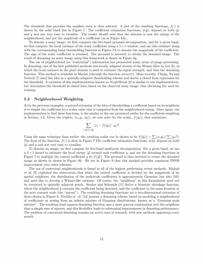
The threshold that provides the smallest error is then selected. A plot of the resulting functions, f(·) isshown by the solid black line in Figure 7. The coefficient estimation functions, x(y), depend on both |y|and y and not very easy to visualize. The reader should note that the abscissa is now the energy of theneighborhood, and not the amplitude of a coefficient (as in Figure 6A).

To denoise a noisy image, we first compute the five-band pyramid decomposition, and for a given band,we first compute the local variance of the noisy coefficient using a 5× 5 window, and use this estimate alongwith the corresponding band thresholding function in Figure 7A to denoise the magnitude of the coefficient.The sign of the noisy coefficient is retained. The pyramid is inverted to obtain the denoised image. Theresult of denoising an noisy image using this framework is shown in Figure 8g.

The use of neighborhood (or “contextual”) information has permeated many areas of image processing.In denoising, one of the first published methods was locally adapted version of the Weiner filter by Lee [6], inwhich the local variance in the pixel domain is used to estimate the signal strength, and thus the denoisingfunction. This method is available in Matlab (through the function wiener2 ). More recently, Chang, Yu andVetterli [7] used this idea in a spatially-adaptive thresholding scheme and derive a closed form expression forthe threshold. A variation of this implementation known as NeighShrink [8] is similar to our implementation,but determines the threshold in closed form based on the observed noisy image, thus obviating the need fortraining.

5.2 Neighborhood Weighting

As in the previous examples, a natural extension of the idea of thresholding a coefficient based on its neighborsis to weight the coefficient by a scalar value that is computed from the neighborhood energy. Once again, ourimplementation to find these functions, is the similar to the one presented earlier for the coefficient-weightingin Section, 4.2. Given the triplets, (xi,yi, |yi|), we now solve for the scalar, f(|yi|), that minimizes:

∑

i:|yi|=|y|

(xi − f(|yi|) · yi)2.

Using the same technique from earlier, the resulting scalar can be shown to be f(|yi|) =∑

i(xiyi)/∑

i(yi2).

The form of the function, f(·) is show in Figure 7.The coefficient estimation functions, x(y), depend on both|y| and y and not very easy to visualize.

To denoise an image, we first compute its five-band multiscale decomposition. For a given band, we usea 5 × 5 kernel to estimate the local energy |~y| around each coefficient y, and use the denoising functions inFigure 7 to multiply the central coefficient y by f(|~y|). The pyramid is then inverted to create the denoisedimage as shown in shown in Figure 8h. We see in Figure 9 that this method provides consistent PSNRimprovement over other schemes.

The use of contextual neighborhoods is found in all of the highest performing recent methods. Michaket al. [9] exploited the observation that when the central coefficient is divided by the magnitude of itsspatial neighbors, the distribution of the multiscale coefficients is approximately Gaussian (see also [10])and used this to develop a Wiener-like estimate. Of course, the “neighbors” in this formulation need notbe restricted to spatially adjacent pixels. Sendur and Selesnick [11] derive a bivariate shrinkage function,where the neighborhood y contains the coefficient being denoised, and the coefficient in the same location atthe next coarsest scale (the “parent”). The resulting denoising functions are a two-dimensional extension ofthose shown in Figure 6. Portilla et. al. [12] present a denoising scheme based on modeling a neighborhoodof coefficients as arising from an infinite mixture of Gaussian distributions, known as a “Gaussian scalemixture”. The resulting least-squares denoising function uses a more general combination over the neighborsthan a simple sum of squares, and this flexibility leads to substantial improvements in denoising performance.The problem of contextual denoising remains an active area of research, with new methods appearing everymonth.

12

A B

HG

FE

DC

Figure 8: Example image Denoising results. (A) Original Image (B) Noisy Image (13.40dB) (C) Band Thresh-olding (24.45dB) (D) Band Weighting (25.04dB) (E) Coefficient Thresholding (24.97dB) (F) CoefficientWeighting (25.72dB) (G)Neighborhood Thresholding (26.24dB) (H) Neighborhood Weighting (26.60dB).All images have been cropped from the original to highlight the details more clearly.

13

PS

NR

(d

B)

imp

rove

me

nt

ove

r th

e n

ois

y im

ag

e

1 2 3 4 5

1 2 3 4 5

6

8

10

12

14Band Thresholding

Band Weighting

Coeff. ThreshodlingCoeff. Weighting

Nbr. Thresh

Nbr. Weighting

Figure 9: PSNR improvement (in dB) , relative to that of the noisy image. Each group of bars shows theperformance of the six denoising schemes for one of the images shown in the bottom row. All denoisingschemes used the exact same Gaussian white noise sample of standard deviation 60.

6 Statistical Modeling For Optimal Denoising

In order to keep the presentation focused and simple, we have resorted to using a training set of noise-free andnoisy coefficients to learn parameters for the denoising function (such as the threshold or weighting values).In particular, given training pairs of noise-free and noisy coefficients, (xn, yn), we have solved a regression

problem to obtain the parameters of the denoising function: θ = argminθ

∑

n(xn − f(yn; θ) · yn)2. Thismethodology is appealing because it does not depend on models of image or noise, and this directness makesit easy to understand. It can also be useful for image enhancement in practical situations where it mightbe difficult to model the signal and noise. Recently, such an approach [13] was used to produce denoisingresults that are comparable to the state-of-the-art. As shown in that work, the data-driven approach canalso be used to compensate for other distortions such as blurring.

But there are two clear drawbacks in the regression approach. First, the underlying assumption of sucha training scheme is that the ensemble of training images is representative of all images. But some of thephotographic image properties we’ve described, while general, do vary significantly from image to image, andit is thus preferable to adapt the denoising solution to the properties of the specific image being denoised.Second, the simplistic form of training we have described requires that the denoising functions must beseparately learned for each noise level. Both of these drawbacks can be somewhat alleviated by consideringa more abstract probabilistic formulation.

14

6.1 The Bayesian View

If we consider the noise-free and noisy coefficients, x and y, to be instances of two random variables X andY respectively, we may rewrite the mean squared error criterion

∑

n

(xn − g(yn))2 ≈ EX,Y (X − g(Y ))2

=

∫

dX

∫

dY P (X,Y )(X − g(Y ))2

=

∫

dX P (X)︸ ︷︷ ︸

Prior

∫

dY P (Y |X)︸ ︷︷ ︸

Noise Model

(X − g(Y ))2︸ ︷︷ ︸

Loss function

(8)

where EX,Y (·) indicates the expected value, taken over random variables X and Y .As described earlier in Section 4.2, the denoising function, g(Y ), that minimizes this expression is the

conditional expectation E(X|Y ). In the framework described above, we have replaced all our samples (xn, yn)by their probability density functions. In general, the prior, P (X), is the model for multiscale coefficientsin the ensemble of noise-free images. The conditional density, P (Y |X), is a model for the noise corruptionprocess. Thus, this formulation cleanly separates the description of the noise from the description of theimage properties, allowing us to learn the image model, P (X), once and then re-use it for any level or typeof noise since (P (Y |X) need not be restricted to additive white Gaussian). The problem of image modelingis an active area of research, and is described in more detail in Chapter 9.

6.2 Empirical Bayesian Methods

The Bayesian approach, assumes that we know (or have learned from a training set) the densities P (X) andP (Y |X). While the idea of a single prior, P (X), for all images in an ensemble is exciting and motivatesmuch of the work in image modeling, denoising solutions based on this model are unable to adapt to thepeculiarities of a particular image. The most successful recent image denoising techniques are based onempirical Bayes methods. The basic idea is define a parametric prior P (X; θ) and adjust the parameters, θ,for each image that is to be denoised. This adaptation can be difficult to achieve, since one generally hasaccess only to the noisy data samples, Y , and not the noise-free samples, X. A conceptually simple methodis to select the parameters that maximize the probability, but this utilizes a separate criterion (likelihood)for the parameter estimation and denoising, and can thus lead to suboptimal results. A more abstract butmore consistent method relies on optimizing Stein’s unbiased risk estimator (SURE) [14–17].

7 Conclusions

The main objective of this chapter was to lead the reader through a sequence of simple denoising techniques,illustrating how observed properties of noise and image structure can be formalized statistically and usedto design and optimize denoising methods. We presented a unified framework for multiscale denoising ofthe form x(∗) = f(∗) · y, and developed three different versions, each one using a different definition for ∗.The first was a global model in which entire bands of multiscale coefficients were modified using a commondenoising function, while the second was a local technique in which each individual coefficient was modifiedusing a function that depended on its own value. The third approach adopted a compromise between thesetwo extremes, using a function that depended on local neighborhood information to denoise each coefficient.For each of these denoising schemes, we presented two variations: a thresholding operator and a weightingoperator.

An important aspect of our examples that we discussed only briefly is the choice of image representa-tion. Our examples were based on an overcomplete multi-scale decomposition into octave-width frequencychannels. While the development of orthogonal wavelets has had a profound impact on the application ofcompression, the artifacts that arise from the critical sampling of these decompositions are higly visible and

15

detrimental when they are used for denoising. Since denoising generally less concerned about the economyof representation (and in particular, about the number of coefficients), it makes sense to relax the criticalsampling requirement, sampling subbands at rates equal to or higher than their associated Nyquist limits. Infact, it has been demonstrated repeatedly (e.g., [18]) and recently proven [17] that redundancy in the imagerepresentation can lead directly to improved denoising performance. There has also been significant effort indeveloping multiscale geometric transforms such as Ridgelets, Curvelets, and Wedgelets which aim to providebetter signal compaction by representing relevant image features such as edges and contours. And althoughthis chapter has focused on multiscale image denoising, there have also been significant improvements indenoising in the pixel domain [19].

The three primary components of our the general statistical formalism of Eq. (8) – signal model, noisemodel, and error function – are all active areas of research. As mentioned previously, statistical modelingof images is discussed in Chapter 9. Regarding the noise, we’ve assumed an additive Gaussian model,but the noise that contaminates real images is often correlated, non-Gaussian, and even signal-dependent.Modeling of image noise is described in Chapter 7. And finally, there is room for improvement in the choiceof objective function. Throughout this chapter, we minimized the error in the pyramid domain, but alwaysreported the PSNR results in the image domain. If the multiscale pyramid is orthonormal, minimizingerror in the multiscale domain is equivalent to minimizing error in the pixel domain. But in over-completerepresentations, this is no longer true, and noise that starts out white in the pixel domain is correlated in thepyramid domain. Recent approaches in image denoising attempt to minimize the mean-squared error in theimage domain while still operating in an over-complete transform domain [13,17]. But even if the denoisingscheme is designed to minimize PSNR in the pixel domain, it is well known that PSNR does not provide agood description of perceptual image quality (see Chapter 20). An important topic of future research is thusto optimize denoising functions using a perceptual metric for image quality [20].

8 Acknowledgments

All photographs used for training and testing were taken by Nicolas Bonnier. We thank Martin Raphan andSiwei Lyu for their comments and suggestions on the presentation of the material in this chapter.

References

[1] E. H. Adelson, C. H. Anderson, J. R. Bergen, P. J. Burt, and J. M. Ogden, “Pyramid methods in imageprocessing,” RCA Engineer, vol. 29, no. 6, pp. 33–41, 1984.

[2] P. J. Burt and E. H. Adelson, “The laplacian pyramid as a compact image code,” IEEE Transactionson Communications, vol. COM-31, pp. 532–540, Apr. 1983.

[3] D. L. Donoho and I. M. Johnstone, “Ideal spatial adaptation by wavelet shrinkage,” Biometrika, vol. 81,no. 3, pp. 425–455, 1994.

[4] D. L. Donoho and I. M. Johnstone, “Adapting to unknown smoothness via wavelet shrinkage,” Journalof the American Statistical Association, vol. 90, no. 432, pp. 1200–1224, 1995.

[5] E. P. Simoncelli and E. H. Adelson, “Noise removal via bayesian wavelet coring,” in Image Processing,1996. Proceedings., International Conference on (E. Adelson, ed.), vol. 1, pp. 379–382 vol.1, 1996.

[6] J. S. Lee, “Digital image enhancement and noise filtering by use of local statistics,” vol. PAMI-2,pp. 165–168, March 1980.

[7] S. G. Chang, B. Yu, and M. Vetterli, “Spatially adaptive wavelet thresholding with context modelingfor image denoising,” Image Processing, IEEE Transactions on, vol. 9, no. 9, pp. 1522–1531, 2000.

16

[8] G. Chen, T. Bui, and A. Krzyzak, “Image denoising using neighbouring wavelet coefficients,” in Acous-tics, Speech, and Signal Processing, 2004. Proceedings. (ICASSP ’04). IEEE International Conferenceon (T. Bui, ed.), vol. 2, pp. ii–917–20 vol.2, 2004.

[9] M. Kivanc Mihcak, I. Kozintsev, K. Ramchandran, and P. Moulin, “Low-complexity image denoisingbased on statistical modeling of wavelet coefficients,” Signal Processing Letters, IEEE, vol. 6, no. 12,pp. 300–303, 1999.

[10] D. L. Ruderman and W. Bialek, “Statistics of natural images: Scaling in the woods,” Phys. Rev. Letters,vol. 73, no. 6, pp. 814–817, 1994.

[11] L. Sendur and I. W. Selesnick, “Bivariate shrinkage functions for wavelet-based denoising exploitinginterscale dependency,” Signal Processing, IEEE Transactions on, vol. 50, no. 11, pp. 2744–2756, 2002.

[12] J. Portilla, V. Strela, M. Wainwright, and E. Simoncelli, “Image denoising using scale mixtures ofgaussians in the wavelet domain,” Image Processing, IEEE Transactions on, vol. 12, no. 11, pp. 1338–1351, 2003.

[13] Y. Hel-Or and D. Shaked, “A discriminative approach for wavelet denoising,” Image Processing, IEEETransactions on, vol. 17, no. 4, pp. 443–457, 2008.

[14] D. L. Donoho, “Denoising by soft-thresholding,” IEEE Trans. Info. Theory, vol. 43, pp. 613–627, 1995.

[15] J. C. Pesquet and D. Leporini, “A new wavelet estimator for image denoising,” in 6th InternationalConference on Image Processing and its Applications, (Dublin, Ireland), pp. 249–253, July 1997.

[16] F. Luisier, T. Blu, and M. Unser, “A new SURE approach to image denoising: Interscale orthonormalwavelet thresholding,” IEEE Trans. Image Proc., vol. 16, March 2007.

[17] M. Raphan and E. P. Simoncelli, “Optimal denoising in redundant bases,” IEEE Trans Image Processing,vol. 17, pp. 1342–1352, aug 2008.

[18] R. R. Coifman and D. L. Donoho, “Translation-invariant de-noising,” in Wavelets and statistics (A. An-toniadis and G. Oppenheim, eds.), San Diego: Springer-Verlag lecture notes, 1995.

[19] K. Dabov, A. Foi, V. Katkovnik, and K. Egiazarian, “Image denoising by sparse 3-d transform-domaincollaborative filtering,” Image Processing, IEEE Transactions on, vol. 16, no. 8, pp. 2080–2095, 2007.

[20] S. S. Channappayya, A. C. Bovik, C. Caramanis, and R. W. Heath, “Design of linear equalizers opti-mized for the structural similarity index,” Image Processing, IEEE Transactions on, vol. 17, pp. 857–872,June 2008.

17