MULTISCALE ANALYSIS OF SPECTRAL BROADENING OFACOUSTIC WAVES BY A TURBULENT SHEAR LAYER ∗

JOSSELIN GARNIER† , ETIENNE GAY‡ , AND ERIC SAVIN§

Abstract. We consider the scattering of acoustic waves emitted by an active source above aplane turbulent shear layer. The layer is modeled by a moving random medium with small spatialand temporal fluctuations of its mean velocity, and constant density and speed of sound. We developa multi-scale perturbative analysis for the acoustic pressure field transmitted by the layer and deriveits power spectral density when the correlation function of the velocity fluctuations is known. Ouraim is to compare the proposed analytical model with some experimental results obtained for jet flowsin open wind tunnels. We start with the Euler equations for an ideal fluid flow and linearize themabout an ambient, unsteady inhomogeneous flow. We study the transmitted pressure field withoutfluctuations of the ambient flow velocity to obtain the Green’s function of the unperturbed mediumwith constant characteristics. Then we use a Lippmann-Schwinger equation to derive an analyticalexpression of the transmitted pressure field, as a function of the velocity fluctuations within thelayer. Its power spectral density is subsequently computed invoking a stationary-phase argument,assuming in addition that the source is time-harmonic and the layer is thin. We finally study theinfluence of the source tone frequency and ambient flow velocity on the power spectral density of thetransmitted pressure field and compare our results with other analytical models and experimentaldata.

Key words. Aeroacoustics, shear layer, scattering, spectral broadening.

1. Introduction. Wave propagation in random media has been extensively stu-died in the literature. When the random inhomogeneities are small it can be analyzedby perturbation techniques. The most efficient approaches are based on techniquesof separation of scales as introduced by e.g. Papanicolaou and his coauthors [2].It is found that the coherent (mean) wave amplitude decreases with the distancetraveled, since wave energy is converted to incoherent fluctuations. The coherent waveexperiences a deterministic spreading and a random time shift. These phenomena wereoriginally described by O’Doherty and Anstey in a geophysical context [34], and werestudied mathematically in [1, 14]. The incoherent wave intensity can be calculatedapproximatively from a transport equation which has the form of a linear radiativetransport equation [25,38].

Research on wave propagation in randomly heterogeneous media has long beenmotivated by communication and imaging problems. Geosciences were the first totake an interest in imaging in random media, typically source and reflector localiza-tion [2, 7]. The objective was to better understand the interactions of waves withthe medium in order to design and implement efficient imaging techniques. As thecoherent wave decays exponentially with the propagation distance, the relevant infor-mation is carried by the covariance function or second-order moment of the incoherentwave field. It turns out that this covariance function was also intensively studied forthe interpretation and analysis of time-reversal experiments [17–19]. As a result theanalysis and understanding of the correlation properties of incoherent wave fields has

∗Submitted to the editors March 10, 2020.Funding: This work was partly funded by DGA/DS Mission pour la Recherche et l’Innovation

Scientifique under grant 2015-60-0060.†Centre de Mathematiques Appliquees, Ecole Polytechnique, FR-91128 Palaiseau cedex, France

(josselin.garnier@polytechnique.edu).‡ONERA/DAAA, Universite Paris-Saclay, FR-92322 Chatillon, France (etienne.gay@vo2-

group.com).§ONERA/DTIS, Universite Paris-Saclay, FR-91123 Palaiseau, France (eric.savin@onera.fr).

1

arX

iv:2

003.

0401

7v1

[ph

ysic

s.fl

u-dy

n] 9

Mar

202

0

2 J. GARNIER, E. GAY, AND E. SAVIN

made significant progress in the recent years and is now the basis of many moderncorrelation-based imaging techniques [5, 6, 21].

This interest is not limited to a fixed environment, since in multiple fields the prop-agation of waves in a moving heterogeneous medium is an important phenomenon.In aeroacoustics for example, tests are performed in open jet wind tunnel in orderto measure the acoustic signature of an active source. In these experiments acousticwaves are transmitted by some device inside the flow, and then received by micro-phones outside the flow. The velocity difference between the jet and the test chamberinduces a turbulent shear layer, and therefore the acoustic waves interact with itand undergo several effects, such as phase and amplitude modulation. Their energyis spread over the frequency band–this is so-called spectral broadening or haystack-ing effect. Interactions between acoustic waves and turbulent shear layers have beenstudied in the literature. Candel et al. [10–12] for example conducted in the seven-ties a series of experiments which primarily motivated this research. These authorswere particularly interested in the power spectral density (PSD) of the pressure fieldtransmitted through the shear layer. Indeed, beyond its ballistic part, i.e. the directunscattered wave component, the transmitted pressure field has multiply scatteredcomponents that result from the interactions with the large turbulent eddies of theshear layer. Some properties of the shape of the induced PSD were deduced, in partic-ular for the two lobes observed on each side of the central peak located at the emissionfrequency of the source. The earlier observations made by Candel et al. [10–12] on thisspectral broadening effect were the starting point of more recent experiments tryingto reproduce it, as for example Krober et al. [27] or Sijtsma et al. [39].

Analytical models for the scattered pressure field transmitted by a shear layerand its PSD were developed in [22, 24] for example. They were based on Lighthill’swave equation [23, Section 2.2] derived in [28] with secondary source terms induced bythe interaction of an incident wave field with turbulent velocity fluctuations. In [8,9]mean-flow refraction effects were considered by modeling the shear layer as an oscillat-ing vortex sheet, and assuming that turbulence induces a random phase modulation ofthe field. Regarding computational experiments, Ewert et al. [15] numerically simu-lated the propagation of acoustic waves in a shear layer with a mean velocity gradientand turbulent velocity fluctuations considering the linearized Euler’s equations andPierce’s convected wave equation [35]. The turbulent velocity fluctuations are numer-ically synthesized by filtering a white noise to impose prescribed statistical propertiesto the turbulent velocity. They are then added to the steady mean flow to forman unsteady ambient flow around which the Euler’s equations are linearized. Theyconcurrently developed an analytical model of acoustic wave scattering based on aperturbative analysis of Lilley’s equation [23, Section 1.2] derived in [29], which wasfurther detailed in [32, 33, 36]. A key aspect of both approaches is a proper choice ofthe correlation function of the turbulent velocity fluctuations which is used to describestatistically the turbulence in the shear layer. In these works, the PSD of the acous-tic pressure field transmitted by the shear layer shows the two sidebands around theemission frequency mentioned above, but some essential features fail to be reproducedby numerical simulations. Clair and Gabard [13] performed numerical simulations ofacoustic wave scattering by a turbulent shear layer by the same methodology. A uni-form mean flow was chosen. They studied in particular the influence of the sourcefrequency, the turbulence convection velocity, and the direction of the observation (theangle between the line from the source location to the measurement location and themean flow direction) on the shape of the PSD of the scattered pressure. The turbulentzone is typically seen as a single large scale eddy by low frequency acoustic waves, as

SPECTRAL BROADENING BY A TURBULENT SHEAR LAYER 3

for scattering by a single vortex. As the frequency of the source increases, the finerturbulence eddies play an increased role in the acoustic scattering mechanism. Morerecently, Bennaceur et al. [4] reproduced numerically the spectral broadening effectby Large Eddy Simulations (LES) of the unsteady Navier-Stokes equations. Inflowvelocity perturbations were added to trigger the shear layer transition to a turbulentstate earlier in the simulation. The authors ended up observing a good agreementbetween the simulated PSD of the far-field transmitted pressure and the foregoingexperiments.

In this context we propose to carry out a mathematical study of the pressure fieldtransmitted through a plane turbulent shear layer. The main objective of this analysisis to determine a simple model from first principles that gives quantitive predictionsabout the transmitted pressure field in terms of the various parameters of the problem(jet velocity, correlation time and standard deviation of the velocity fluctuations,tone frequency, etc.) and that allows to reproduce and explain the experimentalobservations, in particular, that gives an analytical formula of the PSD. This paperextends to random flows the analysis of wave propagation phenomena in randomlystratified motionless media developed in [19] and it identifies the main ingredientsthat are necessary to explain the observations about the spectral broadening reportedin the literature.

The paper is organized as follows. Starting from Euler’s equations, we linearizethem about an ambient, unsteady inhomogeneous flow in Sect. 2. This linearizationstep is essential in identifying the acoustic contributions to the overall flow and inderiving their auto-correlation properties. In Sect. 3 an ambient flow with constantdensity, speed of sound, and velocity is considered so that the expression of the Green’sfunction of this ambient flow can be determined. An analytical expression of thepressure field transmitted by the flow is also derived. Then in Sect. 4 we use aLippmann-Schwinger equation to derive the pressure field transmitted by the flowwith small spatial and temporal fluctuations of the ambient velocity, invoking a Born-like (or single-scattering) approximation. The PSD of the transmitted pressure is alsocomputed in order to be able to compare the proposed model with other analyticalor experimental approaches. This is the main result of the paper, which is convenedin Prop. 6.2. To do so we develop a multiple scale analysis in Sect. 5 and use thestationary-phase theorem in Sect. 6. A numerical example is outlined in Sect. 7, beforea summary of this research is finally given in Sect. 8.

2. Linearized Euler equations about an unsteady inhomogeneous flow.The full non-linear Euler equations for an ideal fluid flow in the absence of friction,heat conduction, or heat production are:

d%

dt+ %∇ · v = 0 ,

dv

dt+

1

%∇p = 0 ,

ds

dt= 0 ,

(2.1)

where % is the fluid density, v is the particle velocity, s is the specific entropy, and pis the thermodynamic pressure given by the equation of state p = p#(%, s), where p#

is a function of the density and specific entropy. It arises from the thermodynamic

4 J. GARNIER, E. GAY, AND E. SAVIN

equilibrium of the fluid so it depends on its density and temperature, or entropy. Also:

(2.2)d

dt=

∂

∂t+ v ·∇

is the usual convective derivative following the particle paths.

2.1. Linearization of Euler equations about an ambient flow. Linearizedacoustics equations arise from the previous conservation equations when their vari-ables are expressed as sums of ambient quantities pertaining to the ambient flow(subscript 0), and lower-order acoustic fluctuations (primed quantities):

%(r, t) = %0(r, t) + %′(r, t) ,

v(r, t) = v0(r, t) + v′(r, t) ,

s(r, t) = s0(r, t) + s′(r, t) ,

p(r, t) = p0(r, t) + p′(r, t) ,

(2.3)

where r = (x, z) is the position within the flow, and x is the horizontal coordinatesand z is the vertical coordinate. In such a manner, the ambient quantities satisfy theEuler equations (2.1):

d%0dt

+ %0∇ · v0 = 0 ,

dv0dt

+1

%0∇p0 = 0 ,

ds0dt

= 0 ,

(2.4)

together with the following relations from the equation of state applicable to theambient flow p0 = p#(%0, s0):

∇p0 = c20∇%0 +

(∂p#

∂s

)%0

∇s0 ,

dp0dt

= c20d%0dt

,

(2.5)

where c0 > 0 is the speed of sound in the ambient flow, c20 = (∂p#

∂% )s0 . Here and fromnow on one has redefined the convective derivative as:

(2.6)d

dt=

∂

∂t+ v0 ·∇ ,

that is, the convective derivative within the ambient flow. The primed quantitiessatisfy the linearized Euler equations:

d%′

dt+ %′∇ · v0 + ∇ · (%0v′) = 0 ,

dv′

dt+ v′ ·∇v0 +

1

%0∇p′ − %′

%20∇p0 = 0 ,

ds′

dt+ v′ ·∇s0 = 0 .

(2.7)

In addition, one has from the linearized equation of state:

(2.8) p′ = c20%′ +

(∂p#

∂s

)%0

s′ .

SPECTRAL BROADENING BY A TURBULENT SHEAR LAYER 5

Combining Eq. (2.4), Eq. (2.5), and Eq. (2.8) we arrive at:

d

dt

(p′

%0c20

)+

1

%0c20v′ ·∇p0 + ∇ · v′ − s′ d

dt

[1

%0c20

(∂p#

∂s

)%0

]= 0 ,

dv′

dt+ v′ ·∇v0 +

1

%0∇p′ − p′

(%0c0)2∇p0 −

s′

(%0c0)2

(∂p#

∂s

)%0

∇p0 = 0 ,

ds′

dt+ v′ ·∇s0 = 0 .

(2.9)

Discarding the last terms in s′ in these first two equations because they are of secondorder by the arguments devised in [35], finally yields the system [16] (the last term inthe second equation below is apparently missing in [16, Eq. (2)]):

d

dt

(p′

K0

)+ ∇ · v′ + 1

K0v′ ·∇p0 = 0 ,

dv′

dt+

1

%0∇p′ + v′ ·∇v0 −

p′

%0K0∇p0 = 0 ,

(2.10)

with K0 = %0c20. In terms of the unknowns q := p′

K0(dimensionless pressure) and

u := %0v′ (momentum) it reads:

dq

dt+

1

%0∇ · u+

1

%0K0

(∂p#

∂s

)%0

u · ∇s0 = 0 ,

du

dt+K0∇q + (Tr(Dv0)I3 + Dv0)u+ (∇K0 −∇p0) q = 0 .

(2.11)

Here I3 is the 3× 3 identity matrix, Dv0 stands for the velocity strain matrix withinthe ambient flow, such that (Dv0)jk =

∂v0j∂rk

. Consequently (Dv0)u = u ·∇v0 asusually noted in fluid mechanics textbooks, and Tr(Dv0) = ∇ · v0. In the experiments[10–12, 27, 39] referred to in Sect. 1 where no combustion occurs and temperaturevariations are small, the (cold) jet flow can be considered as a thermally and caloricallyperfect gas, whereby its heat capacities at constant volume and constant pressure cvand cp, respectively, are constant. Therefore by the equation of state of a perfect gasc20 = γ p0%0 where γ =

cpcv

is Laplace’s coefficient, and the above system reduces to:

dq

dt+

1

%0∇ · u = 0 ,

du

dt+K0∇q + (Tr(Dv0)I3 + Dv0)u+ q(γ − 1)∇p0 = 0 .

(2.12)

Combining the latter with Eq. (2.4) we obtain:

dq

dt+

1

%0∇ · u = 0 ,

du

dt+K0∇q + (Tr(Dv0)I3 + Dv0)u− q(γ − 1)%0

dv0dt

= 0 .

(2.13)

2.2. Model of the ambient flow velocity. We define a fluctuation model ofthe ambient flow velocity as follows:

(2.14) v0(t, r) =

{v + εV (t,x, z) z ∈ [−L, 0] ,v elsewhere .

6 J. GARNIER, E. GAY, AND E. SAVIN

Here L > 0 is the width of the random flow, v is the constant ambient flow velocitywhich is parallel to the horizontal coordinates x of r = (x, z), and 0 ≤ ε � 1 is asmall parameter which scales the amplitude of its fluctuations V . This parameteris often called turbulence intensity in the dedicated literature, as it is related to thecomponents of the turbulent kinetic energy. The latter are generally different for eachdirection [10, 27, 39], but it is assumed in the above model that such intensities arecomparable for all directions. The fluctuations of the constant ambient flow velocityin Eq. (2.14) are given by the mean-square stationary random vector (V (t, r); t ∈R, r ∈ R3) with zero mean:

(2.15) E {V (t,x, z)} = 0 .

Its auto-correlation matrix function reads:

(2.16) E {V (t1, r1)⊗ V (t2, r2)} = RV (t1 − t2, r1 − r2)

= R(t1 − t2)δ(x1 − x2 − (t1 − t2)vt)δ(z1 − z2)1[−L,0](z1)

L,

where vt is the horizontal convection velocity of the turbulent structures (eddies) inthe shear layer, and t 7→ R(t) is a 3 × 3 matrix function which describes the auto-correlation in time. Here z 7→ 1I(z) is the characteristic function of the set I suchthat 1I(z) = 1 if z ∈ I, and 0 otherwise; and a ⊗ b stands for the usual tensorproduct of vectors a and b such that (a⊗ b)ij = aibj in Cartesian coordinates. Thelayer is supported in the region z ∈ [−L, 0] with −L ≤ 0. This model means that thefluctuations V are delta-correlated in space in the local frame moving at the turbulentvelocity vt. The delta function can be seen as the limit of a smooth (for instance,Gaussian) auto-correlation function when the correlation length is smaller than theacoustic wavelength.

3. Transmitted fields without fluctuation of the ambient flow velocity.We start by considering the problem (2.13) without fluctuation of the ambient flowvelocity. In this section we give the expression of the Green’s function for this problem.Thus, we consider general source terms s = (h,f) on the right hand-side of (2.13)with ε = 0, c.f. (2.14), as follows:

dq

dt+

1

%0∇ · u =

h

K0,

du

dt+K0∇q = %0f .

(3.1)

Here h/c20 (remember that K0 = %0c20) corresponds to a specific mass flow rate having

dimension of a density per second, and f corresponds to an acceleration exerted onthe fluid. The convective derivative (2.6) with the model (2.14) is:

(3.2)d

dt=

∂

∂t+ v ·∇ .

For the time being we consider the following specific Fourier transform and its inversewith respect to the time t and the horizontal spatial coordinates x:

(3.3) τ(ω,κ, z) =

∫∫eiω(t−κ·x) τ(t,x, z) dtdx ,

SPECTRAL BROADENING BY A TURBULENT SHEAR LAYER 7

0

zs

f

z

−L

V t xv

v

+ε ( , , )z

v

Fig. 1. Acoustic waves in an homogeneous or random flow of typical thickness L and ambientvelocity v. The emitting sources f are centered at some zs ≥ 0.

and:

(3.4) τ(t,x, z) =1

(2π)3

∫∫e−iω(t−κ·x) τ(ω,κ, z)ω2 dωdκ .

We note from this definition that κ is thus homogeneous to an inverse speed, orslowness. Therefore it is referred to as the (horizontal) slowness vector. Also theinverse Fourier transform with respect to that slowness vector solely will be consideredin the subsequent analysis:

(3.5) τ(ω,x, z) =1

(2π)2

∫eiωκ·x τ(ω,κ, z)ω2dκ .

Taking the Fourier transform (3.3) of the system (3.1) yields:

−iωβ(κ)q +iω

%0κ · ux +

1

%0

∂uz∂z

=h

K0,

−iωβ(κ)ux + iωK0qκ = %0fx ,

−iωuz +K0∂q

∂z= %0fz ,

(3.6)

with the definition (v = (vx, 0)):

(3.7) β(κ) := 1− κ · vx

8 J. GARNIER, E. GAY, AND E. SAVIN

and f = (fx, fz). Eliminating ux in the above one obtains:

∂uz∂z

= iωK0ζ(κ)2q +1

c20h+

%0β(κ)

κ · fx ,

∂q

∂z=

iω

K0uz +

1

c20fz ,

(3.8)

where for β(κ) 6= 0:

(3.9) ζ(κ) =

√β(κ)

c20− |κ|

2

β(κ)

is homogeneous to a slowness. We have thus arrived at a system of ordinary differentialequations for the scalar unknowns (q, uz). Its properties may be first analyzed byconsidering the homogeneous differential system:

(3.10)∂

∂z

(quz

)= iωζ

[0 1

K0ζ

K0ζ 0

](quz

).

Let I0(κ) = K0ζ(κ) be the acoustic impedance and:

(3.11) M0 =

[I

120 I

− 12

0

I120 −I−

12

0

],

[0 I−10

I0 0

]= M−1

0

[1 00 −1

]M0 .

Then the foregoing homogeneous system is diagonalized as:

(3.12)∂

∂zM0

(quz

)= iωζ

[1 00 −1

]M0

(quz

).

This introduces the upward and downward wave mode amplitudes a and b definedsuch that:

(3.13) M0

(quz

)=

[e+iωζ(κ)z 0

0 e−iωζ(κ)z

](ab

).

The latter then satisfy:

(3.14)∂

∂z

(ab

)= 0 ,

which means that these wave mode amplitudes are independent of z away from thesource position. When ζ(κ) is real the wave modes are propagating, a is the amplitudeof the upward propagating mode, and b is the amplitude of the downward propagatingmode. When ζ(κ) is imaginary the wave modes are evanescent (i.e. they decayexponentially with the propagation distance). Here we are interested in the far fieldexpression of the wave so we can restrict our attention to the propagating modes.Eq. (3.9) shows that, when v = 0, ζ(κ) is real if and only if c0|κ| ≤ 1. When v 6= 0but the Mach number M = |v|/c0 < 1, the κ-domain where ζ(κ) is real is morecomplicated, but it contains the disk c0|κ| ≤ 1

1+M . We only consider subsonic flowswith low Mach numbers in the subsequent developments, thus the condition M < 1will always be fulfilled. We can now state the main result of this section, that givesthe expression of the Green’s function in absence of fluctuation of the ambient flowvelocity in terms of upward and downward wavenumber components.

SPECTRAL BROADENING BY A TURBULENT SHEAR LAYER 9

Proposition 3.1 (Solution of Eq. (3.1) and Eq. (3.6)). The solution p =

(qu

)of Eq. (3.1) with the source term s =

(hf

)reads:

p(t,x, z) = G0 ∗ s(t,x, z)

=

∫∫∫G0(t− t′,x− x′, z − z′)s(t′,x′, z′)dt′dx′dz′ ,(3.15)

where

(3.16) G0(t,x, z) = G+0 (t,x, z) H(z) +G−0 (t,x, z)(1−H(z))

is the Green’s function expressed in terms of the Green’s function for upward (+) anddownward (−) waves

(3.17) G±0 (t,x, z) =%0

2(2π)3

∫∫eiω(κ·x±ζ(κ)z−t) g±0 (κ)⊗ g±0 (κ)ω2dωdκ ,

the Heaviside step function z 7→ H(z) (such that H(z) = 1 if z ≥ 0 and H(z) = 0otherwise), and the (generalized) eigenvectors of propagation:

(3.18) g±0 (κ) =1√ζ(κ)

1/K0

κ/β(κ)±ζ(κ)

.

For point sources located at the depth zs ∈ [−L, 0] with forcing terms S(t,x):

(3.19) s(t,x, z) = S(t,x)δ(z − zs) , S =

HF xFz

,

the solution:

(3.20) p =

quxuz

of the system (3.6) in the Fourier domain reads for any z ∈ (−L, zs):

p(ω,κ, z) =1

2e−iωζ(κ)(z−zs) %0 S−(ω,κ)g−0 (κ) ,(3.21)

where S−(ω,κ) = g−0 (κ) · S(ω,κ).

Remark. In (3.17) the integral is over all κ in R2. For κ such that ζ(κ) isimaginary, the sign of the square root of (3.9) which gives rise to an exponentiallydecaying function in (3.17) is selected. We are, however, interested only in the far-fieldexpression, so it is possible to restrict the integral over the κ-domain where ζ(κ) isreal-valued.

Proof. We specify the source s(t, r), considering that it is located at the depthzs and generates forcing terms F (t,x) = (F x(t,x), Fz(t,x)) and H(t,x) such that:

(3.22) f(t,x, z) = F (t,x)δ(z − zs) , h(t,x, z) = H(t,x)δ(z − zs) .

10 J. GARNIER, E. GAY, AND E. SAVIN

Then the vertical momentum uz and pressure q from Eq. (3.8) satisfy the jump con-ditions:

uz(ω,κ, z+s )− uz(ω,κ, z−s ) =

1

c20H(ω,κ) +

%0β(κ)

κ · F x(ω,κ) ,

q(ω,κ, z+s )− q(ω,κ, z−s ) =1

c20Fz(ω,κ) .

(3.23)

Consequently, the upward and downward propagating mode amplitudes of Eq. (3.13)satisfy the jump conditions:

a(ω,κ, z+s )− a(ω,κ, z−s ) = %0 e−iωζ(κ)zs Sa(ω,κ) ,

b(ω,κ, z+s )− b(ω,κ, z−s ) = %0 e+iωζ(κ)zs Sb(ω,κ) ,(3.24)

with the source contributions given by:

(3.25)

(Sa(ω,κ)Sb(ω,κ)

)= K−10 M0

(Fz(ω,κ)

H(ω,κ) + K0

β(κ)κ · F x(ω,κ)

).

One thus deduces that:(3.26)(

ab

)(ω,κ, z) = %0 H(z − zs)

[e−iωζ(κ)zs 0

0 e+iωζ(κ)zs

](SaSb

)(ω,κ) +

(AB

)(ω,κ) ,

where A and B are functions of ω and κ independent of z determined by the boundaryconditions imposed on the wave modes. They specify the wave forms impinging theambient flow (2.14) at its boundaries z = −L and z = 0 if the source lies withinit [20], −L < zs < 0, or z = −L and z = zs ≥ 0 if the source lies outside it [19]. Inagreement with the experiments we have in mind, we will consider in the subsequentdevelopments that the second situation rather takes place; see Fig. 2. However, forthe construction of the Green’s function pertaining to the ambient flow, let us firstconsider that −L < zs < 0. Assuming that no energy is coming upward from z = −∞or downward from z = +∞, translates into the radiation conditions:

(3.27) a(ω,κ,−L) = b(ω,κ, 0) = 0 .

Thus A = 0 and B = −%0 e+iωζ(κ)zs Sb(ω,κ), and one has with Eq. (3.13):

(quz

)(ω,κ, z) =

1

2e+iωζ(κ)(z−zs)

H(ω,κ)c20I0(κ)

+ %0κ·Fx(ω,κ)β(κ)I0(κ)

+ Fz(ω,κ)c20

H(ω,κ)c20

+ %0κ·Fx(ω,κ)β(κ) + I0(κ)Fz(ω,κ)

c20

H(z − zs)

+1

2e−iωζ(κ)(z−zs)

H(ω,κ)c20I0(κ)

+ %0κ·Fx(ω,κ)β(κ)I0(κ)

− Fz(ω,κ)c20

I0(κ)Fz(ω,κ)c20

− H(ω,κ)c20

− %0κ·Fx(ω,κ)β(κ)

(1−H(z − zs)) .(3.28)

From Eq. (3.6) one has ux = K0

β(κ) qκ away from the source. As a result, after definingthe four-dimensional fields p and S as in the proposition, Eq. (3.28) finally yields:

p(ω,κ, z) =1

2H(z − zs) e+iωζ(κ)(z−zs) %0 g

+0 (κ)⊗ g+0 (κ) S(ω,κ)

+1

2(1−H(z − zs)) e−iωζ(κ)(z−zs) %0 g

−0 (κ)⊗ g−0 (κ) S(ω,κ) ,(3.29)

SPECTRAL BROADENING BY A TURBULENT SHEAR LAYER 11

where the (generalized) eigenvectors of propagation g±0 (κ) are defined by (3.18). Thisresult identifies the Green’s function for upward waves G

+

0 (ω,κ, z − zs), z > zs, andthe Green’s function for downward waves G

−0 (ω,κ, z − zs), z < zs, as:

(3.30) G±0 (ω,κ, z) =

1

2e±iωζ(κ)z %0 g

±0 (κ)⊗ g±0 (κ) .

Since a⊗ b c = (b · c)a for any vector c, b · c being the usual inner product of b andc, the scalars:

S±(ω,κ) = g±0 (κ) · S(ω,κ)

=1√ζ(κ)

(H(ω,κ)

K0+κ · F x(ω,κ)

β(κ)± ζ(κ)Fz(ω,κ)

)(3.31)

then turn out to be the (generalized) coordinates of the forcing terms S on the eigen-vectors of propagation, in the Fourier domain.

0

f

z

−L

v

v

zs

a (0)b (0)

a ( )

( )ab zszs

zs

a −L( )−Lb

v

( ) = 0

( ) = 0zsb ++

−( )−

Fig. 2. Acoustic waves in an homogeneous flow of typical thickness L and ambient velocity v.The emitting sources f are centered at some zs ≥ 0, b is the downward wave mode, and a is theupward wave mode.

4. Transmitted fields with fluctuations of the ambient flow velocity. Wenow turn to the case of an ambient flow with a fluctuating velocity, namely Eq. (2.14)

12 J. GARNIER, E. GAY, AND E. SAVIN

with ε > 0. The system (2.13) reads in this case:

dq

dt+

1

%0∇ · u =

h

K0− εV ·∇q ,

du

dt+K0∇q = %0f − εV ·∇u+ ε%0(γ − 1)

dV

dtq − ε((∇ · V )I3 + DV )u ,

(4.1)

where ddt is the convective derivative (3.2). In view of Prop. 3.1 its solution can be

written as:

p = G0 ∗ (s− εKp) ,(4.2)

where:

(4.3) K =

[K0V ·∇ 0

(1− γ)dVdt

1%0

(∇ · V + V ·∇)I3 + 1%0

DV

].

This is a so-called Lippmann-Schwinger equation [30], of which a solution can formallybe constructed by induction:

(4.4) p(n+1) = p(0) − εG0 ∗Kp(n) =

I4 +

n∑j=1

(−εG0 ∗K)j

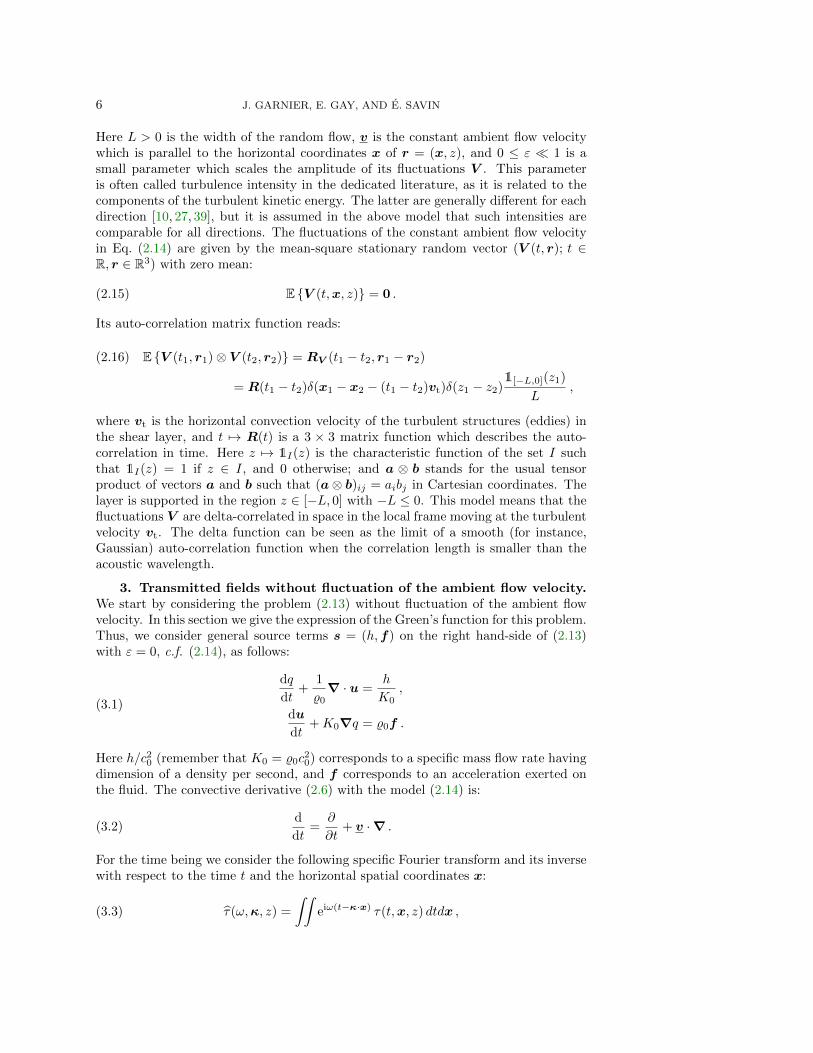
p(0) ,with p(0) := G0 ∗ s. We will focus on the power spectral density (PSD) of p in thesubsequent developments, and more particularly the corrections to the PSD of p(0)

induced by the random fluctuations εV (t, r) of the constant ambient flow velocity v.The leading correction term is proportional to ε2 as we will see below. Therefore, theabove expansion is truncated at order 2 because it is anticipated that higher orderterms will be negligible:

(4.5) p ' p(2) = p(0) − εG0 ∗Kp(0) + ε2 (G0 ∗K)2p(0) .

We note for convenience:

(4.6) p(01) = G0 ∗Kp(0) , p(02) = (G0 ∗K)2p(0) ,

the first-order and second-order terms, respectively, in the expansion of p about theunperturbed, or ballistic pressure/momentum fields p(0) solving Eq. (3.1). Fig. 3sketches the zeroth, first, and second order contributions to the perturbative expansion(4.5), where p(01) corresponds to the waves that have been scattered once by therandom heterogeneities of the ambient flow velocity v, and p(02) corresponds to thewaves that have been scattered twice. All these quantities are the combinations ofupward and downward fields. We show on Fig. 3 only the downward fields, i.e. thetransmitted fields for z ≤ −L.

Regarding the first-order perturbation p(01), we have explicitly:

(4.7) p(01)(t,x, z) =

∫∫∫G0(t− t′,x− x′, z − z′)Kp(0)(t′,x′, z′)dt′dx′dz′ .

The second-order perturbation p(02) is expressed similarly by iterating the convolutionproduct. As will be seen in the following Sect. 5, the first-order contribution in thisproposed perturbative model is responsible for the spectral broadening effect depictedin [10–12]. Therefore we will mainly focus on this term in the following analysis. Wecan now state the main result of this section, that gives the expression of the single-scattered wave in terms of the velocity perturbations.

SPECTRAL BROADENING BY A TURBULENT SHEAR LAYER 13

−L

V t xv

v

+ε ( , , )z

v

z

zs = 0+

o

o

p p p(0) (01) (02)

Fig. 3. Zeroth (ballistic), first, and second order perturbations in the second-order expansionof the transmitted pressure/momentum fields.

Proposition 4.1. Assume the forcing terms are point sources as in Prop. 3.1with zs = 0+. Then the first-order transmitted perturbations p(01) in the perturbativeexpansion (4.4) are given by:

p(01)(ω,κ, z) =%20 e−iωζ(κ)z

4(2π)3

(∫∫∫eiωσ(ω,κ,ω

′,κ′)z′ c(ω,κ, ω′,κ′) · V (ω′,κ′, z′)

×S−(ω − ω′, ωκ− ω

′κ′

ω − ω′

)ω′2dω′dκ′dz′

)g−0 (κ) ,(4.8)

where S− is the generalized coordinate given by Eq. (3.31), and the slowness σ is givenby:

(4.9) σ(ω,κ, ω′,κ′) = ζ(κ)−(

1− ω′

ω

)ζ

(ωκ− ω′κ′

ω − ω′

).

The vector c(ω,κ, ω′,κ′) is:

(4.10) c(ω,κ, ω′,κ′) = k(ω,κ, ω′,κ′)− iωσ(ω,κ, ω′,κ′)d(ω,κ, ω′,κ′)

where K0 = diag(K0,1%0I3), and k(ω,κ, ω′,κ′) and d(ω,κ, ω′,κ′) are given by:

(4.11) k(ω,κ, ω′,κ′) =1

%0K0ζ

(ωκ− ω′κ′

ω − ω′

)− 12

iω′%0(γ − 1)β(κ′)g1(κ)

+1

%0g1(κ) · g1

(ωκ− ω′κ′

ω − ω′

)(iω′κ′

0

)+

1

%0

(iω′κ′

0

)· g1

(ωκ− ω′κ′

ω − ω′

)g1(κ)

+ g−0 (κ)TK0g−0

(ωκ− ω′κ′

ω − ω′

)kd

(ω − ω′, ωκ− ω

′κ′

ω − ω′

),

14 J. GARNIER, E. GAY, AND E. SAVIN

(4.12) d(ω,κ, ω′,κ′) =1

%0g1(κ) · g1

(ωκ− ω′κ′

ω − ω′

)(01

)+

1

%0

(01

)· g1

(ωκ− ω′κ′

ω − ω′

)g1(κ) ,

respectively, with g−0 defined by (3.18) and

(4.13) kd(ω,κ) = iω

(κ

−ζ(κ)

), g1(κ) =

1√ζ(κ)

(κ/β(κ)−ζ(κ)

).

Proof. In the Fourier domain (3.3), the first-order perturbation reads:

p(01)(ω,κ, z)

=

∫∫eiω(t−κ·x) dtdx

∫∫∫G0(t− t′,x− x′, z − z′)Kp(0)(t′,x′, z′)dt′dx′dz′

=

∫ (∫∫eiω(t−κ·x)G0(t,x, z − z′)dtdx

)(∫∫eiω(t

′−κ·x′)Kp(0)(t′,x′, z′)dt′dx′)dz′

(4.14)

with the changes of variable t − t′ → t and x − x′ → x. The first bracketed termis nothing but G0(ω,κ, z − z′), while the second one is the Fourier transform of aproduct–hence a convolution product in the Fourier domain (3.3). In this setting, theFourier transform of the product of regular functions f(t,x, z) and g(t,x, z) reads:

(4.15) fg(ω,κ, z) =1

(2π)3

∫∫f(ω′,κ′, z) g

(ω − ω′, ωκ− ω

′κ′

ω − ω′, z

)ω′2dω′dκ′ .

Thus it remains to compute the Fourier transform (3.3) of K, which depends on timet and the horizontal spatial coordinates x through V (t,x, z) and its various productswith ∇ = (∇x, ∂z). As for the upper left term K11 = K0V ·∇ of K for instance, wehave:

(4.16) K11f(ω,κ, z) =K0

(2π)3

∫∫ [i(ωκ− ω′κ′) · V x(ω′,κ′, z) + Vz(ω

′,κ′, z)∂z

]× f

(ω − ω′, ωκ− ω

′κ′

ω − ω′, z

)ω′2dω′dκ′ .

Accordingly, the lower left term K21 = (1− γ)dVdt yields:

(4.17) K21f(ω,κ, z) =1

%0(2π)3

∫∫K21(ω′,κ′)V (ω′,κ′, z)

× f(ω − ω′, ωκ− ω

′κ′

ω − ω′, z

)ω′2dω′dκ′ ,

where

(4.18) K21(ω,κ) = iω%0(γ − 1)β(κ)I3,

SPECTRAL BROADENING BY A TURBULENT SHEAR LAYER 15

and the remaining lower right term K22 = 1%0

(∇ · V I3 + V ·∇ + DV ) yields:

(4.19) K22f(ω,κ, z) =1

%0(2π)3

∫∫ [(∂zVz(ω

′,κ′, z) + Vz(ω′,κ′, z)∂z

)I3

+ iωκ · V x(ω′,κ′, z)I3 + V (ω′,κ′, z)⊗(

iω′κ′

0

)+ ∂zV (ω′,κ′, z)⊗

(01

)]

× f(ω − ω′, ωκ− ω

′κ′

ω − ω′, z

)ω′2dω′dκ′ .

We finally apply the foregoing formulas to the calculation of p(01) in Eq. (4.14).Here p(0) is given by Prop. 3.1, Eq. (3.21), which is considered for the case zs = 0+

from now on in view of the application of [10–12] we have in mind. In this situationthe Green’s function G0 is reduced to its downward contribution G−0 in the expressionof p(0) and p(01), as one can see on Fig. 3, and p(0) is such that:

∂zp(0)(ω,κ, z) = −iωζ(κ)p(0)(ω,κ, z) .

This allows us to replace ∂z by −i(ω − ω′)ζ(ωκ−ω′κ′

ω−ω′ ) in the expressions of the Fouriertransforms of K11p

(0) and K22p(0) obtained with the above formulas.

Gathering the foregoing definitions of Eq. (4.16), Eq. (4.17), and Eq. (4.19) onearrives at:

p(01)(ω,κ, z) =%20 e−iωζ(κ)z

4(2π)3

(∫∫∫eiωσ(ω,κ,ω

′,κ′)z′(K(ω,κ, ω′,κ′, z′)

+ D(ω,κ, ω′,κ′, z′))S−(ω − ω′, ωκ− ω

′κ′

ω − ω′

)ω′2dω′dκ′dz′

)g−0 (κ) ,

where K and D are the scalar functions:

K(ω,κ, ω′,κ′, z′) = g−0 (κ)TK0K(ω,κ, ω′,κ′, z′)g−0

(ωκ− ω′κ′

ω − ω′

),

D(ω,κ, ω′,κ′, z′) = g−0 (κ)TK0D(ω,κ, ω′,κ′, z′)g−0

(ωκ− ω′κ′

ω − ω′

),

(4.20)

K0 = diag(K0,1%0, 1%0, 1%0

), and K and D are the 4× 4 matrices:

K(ω,κ, ω′,κ′, z′) =

(kd

(ω − ω′, ωκ− ω

′κ′

ω − ω′

)· V (ω′,κ′, z′)

)I4(4.21)

+

[0 0

K21(ω′,κ′)V (ω′,κ′, z′) K22(ω′,κ′)V (ω′,κ′, z′)

],

D(ω,κ, ω′,κ′, z′) =

[0 0

0 D22(ω′,κ′)∂z′V (ω′,κ′, z′)

],(4.22)

with:

K22(ω′,κ′)V (ω′,κ′, z′) =

(iω′κ′

0

)· V (ω′,κ′, z′)I3 + V (ω′,κ′, z′)⊗

(iω′κ′

0

),

D22(ω′,κ′)∂z′V (ω′,κ′, z′) =

(01

)· ∂z′V (ω′,κ′, z′)I3 + ∂z′V (ω′,κ′, z′)⊗

(01

).

16 J. GARNIER, E. GAY, AND E. SAVIN

But by a straightforward computation:

K(ω,κ, ω′,κ′, z′) = k(ω,κ, ω′,κ′) · V (ω′,κ′, z′) ,

where k is given by Eq. (4.11). Likewise:

D(ω,κ, ω′,κ′, z′) = d(ω,κ, ω′,κ′) · ∂z′V (ω′,κ′, z′) ,

where d is given by Eq. (4.12). Integrating by parts in z′ one has:∫eiωσ(ω,κ,ω

′,κ′)z′ D(ω,κ, ω′,κ′, z′)dz′ =

− iωσ(ω,κ, ω′,κ′)

∫eiωσ(ω,κ,ω

′,κ′)z′ d(ω,κ, ω′,κ′) · V (ω′,κ′, z′)dz′ ,

which, when combined with the foregoing expression of K, gives the claimed result.

5. Computation of the power spectral density. Our aim is to compare theforegoing analytical model with the measurements of [10–12]. Here the experimentalresults are presented in terms of the PSD or mean-square Fourier transform of thepressure field recorded at the interface of a free shear flow when an acoustic pulse isimposed at its opposite interface; see again Fig. 2. The PSD is the Fourier transformof the auto-correlation function (by Wiener-Khintchin theorem). Considering theperturbative model (4.5) elaborated in the previous section, the mean-square Fouriertransforms are computed as:

(5.1) E{p(2)(ω1,κ1, z1)⊗ p(2)(ω2,κ2, z2)

}= p(0)(ω1,κ1, z1)⊗ p(0)(ω2,κ2, z2)

+ ε2p(0)(ω1,κ1, z1)⊗E{p(02)(ω2,κ2, z2)

}+ ε2E

{p(02)(ω1,κ1, z1)

}⊗ p(0)(ω2,κ2, z2)

+ ε2E{p(01)(ω1,κ1, z1)⊗ p(01)(ω2,κ2, z2)

},

where Z stands for the complex conjugate of Z. Indeed, p(0) is deterministic andE {p(01)} = 0 because by Prop. 4.1 p(01) is linear with respect to V , which is suchthat E {V } = 0 by Eq. (2.15).

From now on we assume that the sources S(t,x) are time-harmonic forcing termsemitting at the frequency ω0, which means that:

(5.2) S(ω,κ) = S0(κ)δ(ω − ω0) ,

and therefore p(0)(ω,κ, z) = P(0)

(κ, z)δ(ω − ω0), where P(0)

is deduced straightfor-wardly from Prop. 3.1:

(5.3) P(0)

(κ, z) =1

2e−iω0ζ(κ)z %0 g

−0 (κ)⊗ g−0 (κ) S0(κ) .

Consequently, the first, second, and third terms on the right-hand side of Eq. (5.1)are concentrated at the frequency ω0 of the source in the frequency domain. Thespectral broadening effect described in [10–12] should therefore be explained by thelast term on the right-hand side of Eq. (5.1). Thus this effect stems from the PSD ofp(01) with the perturbative model (4.5). The subsequent analyses are focused on thecomputation of this additional contribution.

SPECTRAL BROADENING BY A TURBULENT SHEAR LAYER 17

We carefully isolate the “slow” part of the forcing terms S0(κ), which is denotedby S0,sl(κ), from its “fast” (highly oscillating) part, which is essentially a phase termexp(−iω0κ · xs) where xs is the horizontal central position of the sources and ω0 isthe emitting (high) frequency of Eq. (5.2); that is:

(5.4) S0(κ) = e−iω0κ·xs S0,sl(κ) .

Such an ansatz will prove useful for the application of a stationary-phase argumentin the following derivations. We can now state the main result of this section, whichgives the expression of the covariance matrix of the single-scattered wave.

Proposition 5.1. The covariance matrix of p(01):

(5.5) Ψ(01)(ω1,x1, z1, ω2,x2, z2) = E{p(01)(ω1,x1, z1)⊗ p(01)(ω2,x2, z2)

}along the vertical line x1 = x2 = 0 has the following form when L→ 0:

(5.6) Ψ(01)(ω1,0, z1, ω2,0, z2) = δ(ω1 − ω2)%40(ω1 − ω0)2ω4

1

16(2π)7

×∫∫∫

dκdκ1dκ2 eiω0φ0(κ1,κ2) K (ω1 − ω0,κ;ω1,κ1, ω1,κ2)

× S−0,sl

(ω1

ω0κ1 +

(1− ω1

ω0

)κ

)S−0,sl

(ω1

ω0κ2 +

(1− ω1

ω0

)κ

)g−0 (κ1)⊗ g−0 (κ2) ,

where φ0 is the overall phase of the transmitted signals:

φ0(κ1,κ2) =− ω1

ω0z1ζ(κ1) +

ω1

ω0z2ζ(κ2)− ω1

ω0xs · κ1 +

ω1

ω0xs · κ2 ,(5.7)

S−0,sl is the generalized coordinate of the ”slow” components of the forcing terms:

(5.8) S−0,sl(κ) = g−0 (κ) · S0,sl(κ) ,

g−0 is defined by (3.18), the kernel K plays a fundamental in the spectral broadening:

(5.9) K (ω,κ;ω1,κ1, ω2,κ2) = c(ω1,κ1, ω,κ)TΣ (ω(1− κ · vt)) c(ω2,κ2, ω,κ) ,

c is defined by (4.10), and Σ is the matrix-valued spectral density of the velocityperturbations:

(5.10) Σ(ω) =

∫R(τ) eiωτ dτ .

Proof. We consider the covariance matrix of p(01):

(5.11) Ψ(01)(ω1,κ1, z1, ω2,κ2, z2) = E{p(01)(ω1,κ1, z1)⊗ p(01)(ω2,κ2, z2)

}.

From the result (4.8) of Prop. 4.1 one has:

(5.12) Ψ(01)(ω1,κ1, z1, ω2,κ2, z2) = %40e−iω1ζ(κ1)z1+iω2ζ(κ2)z2

16(2π)6×[ ∫∫∫

ω′21 dω′1dκ

′1dz′1

∫∫∫ω′22 dω

′2dκ

′2dz′2 eiω1σ(ω1,κ1,ω

′1,κ′1)z′1−iω2σ(ω2,κ2,ω

′2,κ′2)z′2

c(ω1,κ1, ω′1,κ′1)TE

{V (ω′1,κ

′1, z′1)⊗ V (ω′2,κ

′2, z′2)}c(ω2,κ2, ω′2,κ

′2)

S−(ω1 − ω′1,

ω1κ1 − ω′1κ′1ω1 − ω′1

)S−(ω2 − ω′2,

ω2κ2 − ω′2κ′2ω2 − ω′2

)]g−0 (κ1)⊗ g−0 (κ2) ,

18 J. GARNIER, E. GAY, AND E. SAVIN

where the slowness function σ is given by Eq. (4.9). Because the auto-correlationmatrix function of V is given by Eq. (2.16), the covariance matrix of V reads:

E{V (ω1,κ1, z1)⊗ V (ω2,κ2, z2)

}= δ(z1 − z2)

1[−L,0](z1)

L

×∫∫

R(t1 − t2)δ(x1 − x2 − (t1 − t2)vt) eiω1(t1−κ1·x1)−iω2(t2−κ2·x2) dt1dt2dx1dx2

which by the changes of variables τ = t1 − t2, t = 12 (t1 + t2), ρ = x1 − x2, and

x = 12 (x1 + x2) also reads:

(5.13) E{V (ω1,κ1, z1)⊗ V (ω2,κ2, z2)

}=

(2π)3δ(ω1 − ω2)δ(ω1κ1 − ω2κ2)δ(z1 − z2)1[−L,0](z1)

LΣ(ω1(1− κ1 · vt)) ,

where Σ(ω) is defined by (5.10). Inserting Eq. (5.13) into Eq. (5.12) one arrives atthe desired result with the change of variable ω′1 → ω, κ′1 → κ.

But S is given by Eq. (5.2), so that letting L→ 0 yields:

Ψ(01)(ω1,κ1, z1, ω2,κ2, z2) =

%40e−iω1ζ(κ1)z1+iω2ζ(κ2)z2

16(2π)3I(ω1,κ1, ω2,κ2)g−0 (κ1)⊗ g−0 (κ2) ,

where:

(5.14) I(ω1,κ1, ω2,κ2) = δ(ω1 − ω2)(ω1 − ω0)2∫

K (ω1 − ω0,κ;ω1,κ1, ω1,κ2)

× S−0(ω1

ω0κ1 +

(1− ω1

ω0

)κ

)S−0(ω1

ω0κ2 +

(1− ω1

ω0

)κ

)dκ ,

and S−0 (κ) = g−0 (κ) · S0(κ). Lastly, we apply the inverse Fourier transform (3.5)with respect to κ1 and κ2 to the foregoing result in order to get an expression of thecorrelation of the transmitted fields at two points (x1, z1) and (x2, z2). The covariancematrix of p(01) (remind the partial Fourier transform of Eq. (3.5)) thus reads:

Ψ(01)(ω1,x1, z1, ω2,x2, z2) =%40ω

21ω

22

16(2π)7×∫∫

eiω1(κ1·x1−ζ(κ1)z1)−iω2(κ2·x2−ζ(κ2)z2) I(ω1,κ1, ω2,κ2) g−0 (κ1)⊗ g−0 (κ2)dκ1dκ2 .

Accounting for (5.14) together with the ansatz (5.4) and eventually considering thecovariance on the vertical line x1 = x2 = 0 yields the desired result.

In view of Eq. (5.1), the PSD of the ballistic pressure/momentum fields p(0) isalso needed. But these quantities are, again, deterministic and time-harmonic at thefrequency ω0, so that one simply computes:

Ψ(0)(0, z1,0, z2) = P (0)(0, z1)⊗ P (0)(0, z2)

=%20ω

40

4(2π)4

∫∫dκ1dκ2 e−iω0[ζ(κ1)z1−ζ(κ2)z2+κ1·xs−κ2·xs]

× S−0,sl(κ1)S−0,sl(κ2) g−0 (κ1)⊗ g−0 (κ2) ,

(5.15)

SPECTRAL BROADENING BY A TURBULENT SHEAR LAYER 19

reminding the definition (5.3). We finally invoke a stationary-phase argument toconclude on the derivation of the PSD of the transmitted pressure field, with theforegoing expression of the phase. This last step is detailed in the next section.

6. Stationary-phase method. In this section we start by considering the caseM = |v|/c0 � 1 (Mach number of the ambient flow) and eventually choose v ' 0(M ' 0 and β ' 1) to simplify the derivation below. The case M 6= 0 but small will beaddressed in subsequent developments. The first goal is to determine the stationaryslowness vectors κ1,sp and κ2,sp such that:

∇κ1φ0(κ1,sp,κ2,sp) = ∇κ2

φ0(κ1,sp,κ2,sp) = 0 .

Lemma 6.1. In the instance that ω1 and ω2 are equal to ω0 at the first order,namely 1− ω1

ω0= o(1) and 1− ω2

ω0= o(1), one has:

(6.1)

κ1,sp ' ζ(κ1,sp)xsz1

=xs

c0√|xs|2 + z21

, κ2,sp ' ζ(κ2,sp)xsz2

=xs

c0√|xs|2 + z22

.

Proof. ζ(κ) is given by Eq. (3.9) with β(κ) = 1, therefore ∇κζ(κ) = −κ/ζ(κ).Thus:(6.2)

∇κ1φ0(κ1,κ2) =ω1

ω0

[z1

κ1

ζ(κ1)− xs

], ∇κ2φ0(κ1,κ2) = −ω1

ω0

[z2

κ2

ζ(κ2)− xs

].

Then for ω1

ω0= O(1) one obtains the claimed result.

We subsequently apply the stationary-phase theorem to Eq. (5.6) to obtain the fi-nal expression of the PSD of the scattered transmitted pressure field given in Prop. 6.2,which is the main result of the paper.

Proposition 6.2. Let d = (|xs|2 + z2)12 be the distance from the time-harmonic

sound source (5.2) at (xs, 0+) (with S0 = (H0, F 0x, F0z)) to the observation point

(0, z) at the depth z (z < −L) on the outer side of the flow. Then the ballistictransmitted pressure field p′(0) = K0q

(0) has the form:

(6.3) p′(0)(ω,0, z)p′(0)(ω′,0, z) = δ(ω − ω0)δ(ω′ − ω0)Ψ0(xs, z, ω0) ,

with:(6.4)

Ψ0(xs, z, ω0) =%20ω

20

4(2π)2c20d4

∣∣∣∣ d

%0c0H0

(xsc0d

)+ xs · F 0x

(xsc0d

)− zF0z

(xsc0d

)∣∣∣∣2 ,and for 1− ω

ω0= o(1) the mean-square Fourier transform of the scattered transmitted

pressure field p′(01) = K0q(01) reads:

(6.5) E{p′(01)(ω,0, z)p′(01)(ω′,0, z)

}= δ(ω − ω′)Ψ01(xs, z, ω, ω0) ,

where:

(6.6) Ψ01(xs, z, ω, ω0) =%20ω

20

4(2π)3

(1− ω

ω0

)2(ω

ω0

)4

Ψ1(xs, z, ω, ω0)Ψ0 (xs, z, ω0) ,

and Ψ1(xs, z, ω, ω0) is a filtered frequency spectrum responsible for the spectral broad-ening of the source centered about ω0 given by:

(6.7) Ψ1(xs, z, ω, ω0) =

∫|κ|≤ 1

c0

K

(ω − ω0,κ;ω,

xsc0d

, ω,xsc0d

)dκ ,

20 J. GARNIER, E. GAY, AND E. SAVIN

where K is defined by (5.9).

Proof. Expanding the phase (5.7) in a Taylor series about the small incrementω0 − ω1 yields:

(6.8) φ0(κ1,κ2) ' −ω1

ω0z1ζ(κ1) +

ω1

ω0z2ζ(κ2)− ω1

ω0(κ1 − κ2) · xs .

We can thus identify the slow part of the phase φsl from its fast part φf proportionalto ω1/ω0 as follows:

φf(κ1,κ2) =− ζ(κ1)z1 + ζ(κ2)z2 − (κ1 − κ2) · xs ,

φsl(κ1,κ2) =

(1− ω1

ω0

)(z1ζ(κ1) + κ1 · xs − z2ζ(κ2)− κ2 · xs) .

(6.9)

Applying the stationary-phase theorem in dimension n = 4 (see for example [19, Eq.(14.77)]) to the auto-spectrum (5.6) of the first-order perturbations of the transmittedpressure/momentum fields yields:

Ψ(01)(ω1,0, z1, ω2,0, z2) = δ(ω1−ω2)%40(ω1 − ω0)2ω4

1

16ω20(2π)5

ei(n∗−2)π2 eiω0φf(κ1,sp,κ2,sp)√

|det Hκ1,κ2φf(κ1,sp,κ2,sp)|

× eiω0φsl(κ1,sp,κ2,sp)

∫K (ω1 − ω0,κ;ω1,κ1,sp, ω1,κ2,sp)dκ

× S−0,sl (κ1,sp) S−0,sl (κ2,sp) g−0 (κ1,sp)⊗ g−0 (κ2,sp) ,

where n∗ is the number of positive eigenvalues of the Hessian Hκ1,κ2φf(κ1,sp,κ2,sp).The latter is block-diagonal owing to Eq. (6.2) and reads:

Hκ1,κ2φf(κ1,κ2) =

z1ζ(κ1)

(I2 + κ1⊗κ1

ζ(κ1)2

)0

0 − z2ζ(κ2)

(I2 + κ2⊗κ2

ζ(κ2)2

) ,such that:

det Hκ1,κ2φf(κ1,κ2) =

(z1z2

ζ(κ1)ζ(κ2)

)2(1 +

|κ1|2

ζ(κ1)2

)(1 +

|κ2|2

ζ(κ2)2

).

From this we can deduce that the eigenvalues of Hκ1,κ2φf(κ1,κ2) are:

λ1 =z1

ζ(κ1), λ2 =

z1ζ(κ1)

(1 +

|κ1|2

ζ(κ1)2

),

λ3 = − z2ζ(κ2)

, λ4 = − z2ζ(κ2)

(1 +

|κ2|2

ζ(κ2)2

),

and therefore n∗ = 2. Besides:√|det Hκ1,κ2

φf(κ1,sp,κ2,sp)| = c20d21d

22

z1z2

introducing d1 = (|xs|2 + z21)12 and d2 = (|xs|2 + z22)

12 , and:

φf(κ1,sp,κ2,sp) =d2 − d1c0

.

SPECTRAL BROADENING BY A TURBULENT SHEAR LAYER 21

Indeed, owing to Lemma 6.1 one also has:

(6.10) ζ(κ1,sp) =z1c0d1

, ζ(κ2,sp) =z2c0d2

.

We can finally compute the mean-square Fourier transform of the first-order transmit-ted pressure field p′(01) = K0q

(01) as the upper-left term of Ψ(01)(ω1,0, z1, ω2,0, z2),and that of the ballistic transmitted pressure field p′(0) = K0q

(0) as the upper-leftterm of Ψ(0)(0, z1,0, z2). Using Eq. (3.18) with β(κ) = 1 and Eq. (3.31) with thedefinition (5.4), we have:

S−0,sl(κ1,sp) = eiω0c0

|xs|2d1 g−0 (κ1,sp) · S0(κ1,sp) ,

with a similar expression for S−0,sl(κ2,sp); see Eq. (5.8). We end up with:

p′(0)(ω,0, z1)p′(0)(ω′,0, z2) = δ(ω − ω0)δ(ω′ − ω0)eiω0c0

(z22d2− z

21d1

)

4(2π)2%20ω

20

d1d2

× ϕ(xsc0d1

,z1c0d1

)ϕ

(xsc0d2

,z2c0d2

),

and:

E{p′(01)(ω1,0, z1)p′(01)(ω2,0, z2)

}= δ(ω1 − ω2)

eiω0c0

(z22d2− z

21d1

)

16(2π)5%40ω

40

d1d2

×(

1− ω1

ω0

)2(ω1

ω0

)4

Ψ(xs, z1, z2, ω1, ω0)ϕ

(xsc0d1

,z1c0d1

)ϕ

(xsc0d2

,z2c0d2

),

where:

(6.11) Ψ(xs, z1, z2, ω, ω0) = eiω0φsl(κ1,sp,κ2,sp)

×∫|κ|≤ 1

c0

K (ω − ω0,κ;ω,κ1,sp, ω,κ2,sp) dκ ,

and, for S0 = (H0, F 0x, F0z):

ϕ(κ, ζ) =1

K0H0(κ) + κ · F 0x(κ)− ζF0z(κ) .

We thus define:

Ψ0(xs, z, ω0) =%20ω

20

4(2π)2d2

∣∣∣∣ϕ( xsc0d , z

c0d

)∣∣∣∣2for d = (|xs|2 + z2)

12 , and:

Ψ1(xs, z, ω1, ω0) = Ψ(xs, z, z, ω1, ω0) =

∫|κ|≤ 1

c0

K (ω1 − ω0,κ;ω1,κ1,sp, ω1,κ1,sp) dκ ,

then we obtain the claimed formulas (6.4) and (6.6).

22 J. GARNIER, E. GAY, AND E. SAVIN

It remains to compute the integral in Eq. (6.7). Assuming that R(τ) is diagonal,namely R(τ) = R(τ)I3, and denoting by Σ the Fourier transform of R, one has:

K (ω − ω0,κ;ω,κsp, ω,κsp) =

Σ((ω − ω0)(1− vt · κ))c(ω,κsp, ω − ω0,κ) · c(ω,κsp, ω − ω0,κ) ,

with κsp = xs/(c0d). These results are illustrated in the next section for a correlationfunction and parameters adapted from the experiments in [10] and analytical modelsin [33].

7. Numerical example. At first, we choose a Gaussian model for the autocor-relation function τ 7→ R(τ) of Eq. (2.16):

(7.1) R(τ) = R(τ)I3, R(τ) = σ2V exp

(−π τ

2

4τ2s

).

Here τs is the correlation time, or the turbulence integral timescale in the dedicatedliterature, i.e. the typical time scale of a realization of the turbulent velocity fluctua-tions V such that

∫ +∞0

R(τ)/R(0)dτ = τs; and σV quantifies their standard deviation.Then from Eq. (5.10):

(7.2) Σ(ω) = 2τsσ2V exp

(− 1

πτ2sω

2

).

In view of Eq. (2.16) and Eq. (2.14), the variance σ2V scales as a squared velocity–

typically |v|2 the squared mean jet velocity. In order to compare our results ofProp. 6.2 with the experimental results in [10] and the analytical models in e.g. [32,33,36], we plot on Fig. 4 and Fig. 5 the normalized “power spectrum” Ψ2(xs, z, ω0, ω)of the transmitted pressure field defined by:

(7.3) Ψ2(xs, z, ω, ω0) = δ(ω − ω0) +ε2%20

4(2π)3(ω − ω0)2

(ω

ω0

)4

Ψ1(xs, z, ω, ω0)

in dB (ΨdB2 = 10 log10 Ψ2) for the data provided in [31,33]: L = 0.1 m for the thickness

of the turbulent shear layer at a distance D = 0.5 m from the jet in the experimentsof Candel et al. [10], τs = L/|vt|, ε = 12% for the turbulence intensity, |vt| = 0.5|v|for the velocity of the turbulent eddies, and c0 = 340 m/s and %0 = 1.2 kg/m3 forthe ambient flow characteristics. More particularly, Fig. 4 shows Ψ2(0,−L, ω0, ω) as afunction of ∆ω = ω − ω0 for various tone frequencies f0 = ω0/(2π) in the range [6–20]kHz and the jet velocity UJ = |v| = 60 m/s, and Fig. 5 shows Ψ2(0,−L, ω0, ω) as afunction of ∆ω for various jet velocities UJ in the range [20–60] m/s and f0 = 20 kHz.In addition, we show in these figures the analytical results displayed in [33] for thehomogeneous axisymmetric turbulence (HAT), and the three-dimensional Gaussianhomogeneous isotropic turbulence (HIT) correlation functions developed in this work.Both models are based on the general model of isotropic turbulence correlation derivedin [3, 26, 37]. The HAT model takes explicitly into account the axisymmetry of acircular jet. Also the experiments in [10] are for a circular jet with a large radius,so that the plane shear layer model developed here is applicable for a source at thecenter of the jet.

The two lobes of the experimental results shown in Fig. 4(a) and Fig. 5(a) arewell recovered, together with their position on the frequency axis which has been

SPECTRAL BROADENING BY A TURBULENT SHEAR LAYER 23

observed to be independent of the tone frequency f0. Indeed, from the expression ofΨ01(xs, z, ω0, ω) in Prop. 6.2 the maxima of the lobes are approximately found as themaxima of ∆ω2 exp(− 1

π τ2s∆ω2(1−Mt)

2) which yields:

|∆ωmax| '√πc0LMt ,

where Mt = |vt|/c0 � 1 is the (small) Mach number for the turbulent eddies. Thisestimate is in good agreement with [4,10–13,31,32,36,39]. Despite several simplifica-tions, the proposed model allows to recover the main trends of the power spectrumof the transmitted pressure field already outlined in those previous works, namely:

• a linear growth in the position of the maximum of the lobes as a function ofthe velocity of the turbulent eddies Mt. Also the width of the lobes and thusthe amount of scattered energy increases as well when Mt increases;

• the energetic macro-eddies contribute to the larger part of the scattered pres-sure field. Spectral broadening is related to a Doppler shift due to the motionof these large structures which act as secondary sources for the scattered field.

(a) (b)

(c) (d)

Fig. 4. Normalized power spectrum of the transmitted pressure field as a function of thefrequency gap f − f0 for various tone frequencies f0 in the range [6–20] kHz and jet velocityUJ = |v| = 60 m/s: (a) experimental observations from [10]; (b) the results of Prop. 6.2; (c)the model of [33] for a Gaussian homogeneous axisymmetric turbulence (HAT) correlation functionof the fluctuations of the ambient flow velocity; (d) the model of [33] for a Gaussian homogeneousisotropic turbulence (HIT) correlation function of the fluctuations of the ambient flow velocity. Notethat in [33] the notations ω = 2πF and ω0 = 2πf are rather used.

8. Summary and outlook. In this paper we have developed an analyticalmodel of the power spectral density of the acoustic waves transmitted by a plane tur-

24 J. GARNIER, E. GAY, AND E. SAVIN

(a) (b)

(c) (d)

Fig. 5. Normalized power spectrum of the transmitted pressure field as a function of the fre-quency gap f − f0 for various jet velocities UJ = |v| in the range [20-60] m/s and tone frequencyf0 = 20 kHz: (a) experimental observations from [10]; (b) the results of Prop. 6.2; (c) the modelof [33] for a Gaussian-HAT correlation function of the fluctuations of the ambient flow velocity; (d)the model of [33] for a Gaussian-HIT correlation function of the fluctuations of the ambient flowvelocity. Note that in [33] the notations ω = 2πF and ω0 = 2πf are rather used.

bulent shear layer of which ambient velocity is randomly perturbed by weak spatialand temporal fluctuations, when a time-harmonic source acts above it. The analysisstarts from the linearized Euler’s equations written as a Lippmann-Schwinger equa-tion, considering that the fluctuations of the ambient flow velocity act as secondarysources for the transmitted acoustic waves. A Born-like approximate solution of theLippmann-Schwinger equation has been derived to work out a first-order model of thepressure field transmitted by the shear layer. In this model, the transmitted wavesare constituted by their unperturbed components formed by the waves emitted by thesource which have not been scattered by the ambient velocity fluctuations, and theirperturbed components formed by the waves which have typically been scattered onceby those fluctuations. These scattered waves are of particular interest since they havebeen characterized by their PSD in the experiments reported in [10–12], which pri-marily motivated this work. They also motivated the linearization of Euler equationswe have applied since it identifies the acoustic components of interest. Using variousassumptions for the ambient flow (thin layer) and the (high-frequency) source, and astationary-phase argument, a model for the PSD of the scattered waves transmittedby the shear layer has been derived. It exhibits the main properties observed forthe experimental PSD in [10–12, 27, 39], and for the numerically simulated PSD andalternative analytical models in [4, 13,15,31–33,36,39].

SPECTRAL BROADENING BY A TURBULENT SHEAR LAYER 25

The PSD of the pressure field transmitted by the shear layer shows a characteristicspectral broadening effect, whereby a reduction of the main peak at the source tonefrequency in favor of more distributed spectral humps on both sides of the former, isobserved. The main peak arises from the unperturbed transmitted pressure, and side-bands (lobes) arise in connection with a Doppler shift effect due to the motion of theturbulent eddies acting as secondary sources for the scattered transmitted pressure.A linear widening of these lobes with the convection velocity of the turbulent eddieshas been observed, as well as the independence of the location of their maxima withrespect to the tone frequency. Increasing the latter also leads to a widening of the side-bands and higher scattered levels. The proposed analysis has used a delta-correlatedmodel of the turbulent velocity spatial fluctuations and a Gaussian model of its tem-poral fluctuations, though it could be improved by considering correlation modelspertaining to homogeneous isotropic turbulence (HIT) or homogeneous axisymmetricturbulence (HAT) as done in [33]. Specifically, the general model of isotropic turbu-lence correlation derived in [3, 26, 37] could be considered in future works to possiblybetter match experimental observations. However the model retained here has beenable to predict the main features outlined above.

Next steps to investigate to improve our PSD model predictions could be to relaxsome hypotheses such as the thickness of the layer, which is assumed to be infinitelythin. Horizontally stratified flows have been considered here, but axisymmetric flowgeometries have relevance to aerospace applications as well. The source-microphoneaxis was perpendicular to the flow in our analysis. Hence the influence of the angle ofillumination could be studied as in [9, 13, 32, 36]. Besides, measurements and modelsof the cross power spectra between two microphones have been reported in [10–12,24],so that our model could also be compared to these results. Lastly, the velocity of theflow was assumed to be much smaller than the speed of sound. The influence of asignificant Mach number could be explored further.

REFERENCES

[1] D. G. Alfaro Vigo, J.-P. Fouque, J. Garnier, and A. Nachbin. Robustness of time reversal forwaves in time-dependent random media. Stochastic Process. Appl. 113(2), 289-313 (2004).

[2] M. Asch, W. Kohler, G. Papanicolaou, M. Postel, and B. White. Frequency content of randomlyscattered signals. SIAM Rev. 33(4), 519-625 (1991).

[3] G. K. Batchelor. The Theory of Homogeneous Turbulence. Cambridge University Press, Cam-bridge (1953).

[4] I. Bennaceur, D.C. Mincu, I. Mary, M. Terracol, L. Larcheveque, and P. Dupont. Numericalsimulation of acoustic scattering by a plane turbulent shear layer: Spectral broadeningstudy. Comput. Fluids 138, 83-98 (2016).

[5] L. Borcea, G. Papanicolaou, and C. Tsogka, Theory and applications of time reversal andinterferometric imaging. Inverse Problems 19(6), S139-S164 (2003).

[6] L. Borcea, J. Garnier, G. Papanicolaou, and C. Tsogka. Enhanced statistical stability in coher-ent interferometric imaging. Inverse Problems 27(8), 085004 (2011).

[7] R. Burridge, G. Papanicolaou, P. Sheng, and B. White. Probing a random medium with apulse. SIAM J. Appl. Math. 49(2), 582-607 (1989).

[8] L. M. B. C. Campos. The spectral broadening of sound by turbulent shear layers. Part 1. Thetransmission of sound through turbulent shear layers. J. Fluid Mech. 89(4), 723-749 (1978).

[9] L. M. B. C. Campos. The spectral broadening of sound by turbulent shear layers. Part 2. Thespectral broadening of sound and aircraft noise. J. Fluid Mech. 89(4), 751-783 (1978).

[10] S. Candel, A. Guedel, and A. Julienne. Refraction and scattering in an open wind tunnelflow. In Proc. 6th Int. Congress on Instrumentation in Aerospace Simulation FacilitiesICIASF’75, 22-24 September 1975, Ottawa ON. pp. 288-300 (1975).

[11] S. Candel, A. Guedel, and A. Julienne. Radiation, refraction and scattering of acoustic wavesin a free shear flow. Proc. 3rd AIAA Aeroacoustics Conf., 20-23 July 1976, Palo Alto CA.AIAA paper #1976-544 (1976).

26 J. GARNIER, E. GAY, AND E. SAVIN

[12] S. Candel, A. Guedel, and A. Julienne. Resultats preliminaires sur la diffusion d’une ondeacoustique par ecoulement turbulent. J. Phys. Colloques 37(C1), C1-153-C1-160 (1976).

[13] V. Clair and G. Gabard. Numerical investigation on the spectral broadening of acoustic wavesby a turbulent layer. In Proc. 22nd AIAA/CEAS Aeroacoustics Conf., 30 May - 1 June2016, Lyon, France. AIAA paper #2016-2701 (2016).

[14] J.-F. Clouet and J.-P. Fouque. Spreading of a pulse traveling in random media. Ann. Appl.Probab. 4(4), 1083-1097 (1994).

[15] R. Ewert, O. Kornow, B. J. Tester, C. J. Powles, J. W. Delfs, and M. Rose. Spectral broadeningof jet engine turbine tones. In Proc. 14th AIAA/CEAS Aeroacoustics Conf., 5-7 May 2008,Vancouver BC. AIAA paper #2008-2940 (2008).

[16] A. Fannjiang and L. V. Ryzhik. Radiative transfer of sound waves in a random flow: turbulentscattering, straining, and mode-coupling. SIAM J. Appl. Math. 61(5), 1545-1577 (2001).

[17] M. Fink. Time reversed acoustics. Scientific American 281(5), 91-97 (1999).[18] J.-P. Fouque, J. Garnier, A. Nachbin, and K. Sølna. Time reversal refocusing for point source

in randomly layered media. Wave Motion 42(3), 238-260 (2005).[19] J.-P. Fouque, J. Garnier, G. Papanicolaou, and K. Sølna. Wave Propagation and Time Reversal

in Randomly Layered Media. Springer-Verlag, New York NY (2007).[20] J. Garnier. Imaging in randomly layered media by cross-correlating noisy signals. Multiscale

Model. Simul. 4(2), 610-640 (2005).[21] J. Garnier and G. Papanicolaou. Passive Imaging with Ambient Noise. Cambridge University

Press, Cambridge (2016).[22] G. H. Goedecke, R. C. Wood, H. J. Auvermann, V. E. Ostashev, D. I. Havelock, and C. Ting.

Spectral broadening of sound scattered by advecting atmospheric turbulence. J. Acoust.Soc. Am. 109(5), 1923-1934 (2001).

[23] M. E. Goldstein. Aeroacoustics. McGraw-Hill, New York NY (1976).[24] A. Guedel. Scattering of an acoustic field by a free jet shear layer. J. Sound Vib. 100(2), 285-304

(1985).[25] A. Ishimaru. Wave Propagation and Scattering in Random Media, Volume 2: Multiple Scatter-

ing, Turbulence, Rough Surfaces, and Remote Sensing. Academic Press, San Diego (1978).[26] Th. von Karman, L. Howarth. On the statistical theory of isotropic turbulence. Proc. R. Soc.

Lond. A 1938 164, 192-215 (1938).[27] S. Krober, M. Hellmold, and L. Koop. Experimental investigation of spectral broadening of

sound waves by wind tunnel shear layers. In Proc. 19th AIAA/CEAS Aeroacoustics Conf.,27-29 May 2013, Berlin, Germany. AIAA paper #2013-2255 (2013).

[28] M. J. Lighthill. On sound generated aerodynamically: (I) General theory. Proc. R. Soc. Lond.A211(1107), 564-587 (1952).

[29] G. M. Lilley. Generation of sound in a mixing region. In The Generation and Radiation ofSupersonic Jet Noise vol. IV: Theory of Turbulence Generated jet Noise, Noise Radiationfrom Upstream Sources, and Combustion Noise, pp. 2-69. Technical report AFAPL-TR-72-53, Air Force Aero Propulsion Laboratory, Wright-Patterson Air Force Base OH (1972).

[30] B. A. Lippmann and J. Schwinger. Variational principles for scattering processes I. Phys. Rev.79(3), 469-480 (1950).

[31] A. McAlpine, C. J. Powles, and B. J. Tester. A weak-scattering model for tone haystacking. InProc. 15th AIAA/CEAS Aeroacoustics Conf., 11-13 May 2009, Miami, FL. AIAA paper#2009-3216 (2009).

[32] A. McAlpine, C. J. Powles, and B. J. Tester. A weak-scattering model for turbine-tone haystack-ing. J. Sound Vib. 332(16), 3806-3831 (2013).

[33] A. McAlpine and B. J. Tester. A weak-scattering model for tone haystacking caused by soundpropagation through an axisymmetric turbulent shear layer. In Proc. 22nd AIAA Aeroa-coustics Conf., 30 May - 1 June 2016, Lyon, France. AIAA paper #2016-2702 (2016).

[34] R. F. O’Doherty and N. A. Anstey. Reflections on amplitudes. Geophys. Prospect. 19(3), 430-458 (1971).

[35] A. D. Pierce. Wave equation for sound in fluids with unsteady inhomogeneous flow. J. Acoust.Soc. Am. 87(6), 2292-2299 (1990).

[36] C. J. Powles, B. J. Tester, and A. McAlpine. A weak-scattering model for turbine-tone haystack-ing outside the cone of silence. Int. J. Aeroacoustics 10(1), 17-50 (2011).

[37] H. P. Robertson. The invariant theory of isotropic turbulence. Math. Proc. Cambridge Philos.Soc. 36(2), 209-223 (1940).

[38] L. V. Ryzhik, G. Papanicolaou, and J. B. Keller. Transport equations for elastic and otherwaves in random media. Wave Motion 24(4), 327-370 (1996).

[39] P. Sijtsma, S. Oerlemans, T. Tibbe, T. Berkefeld, and C. Spehr. Spectral broadening by shearlayers of open jet wind tunnels. In Proc. 20th AIAA/CEAS Aeroacoustics Conf., 16-20

SPECTRAL BROADENING BY A TURBULENT SHEAR LAYER 27

June 2014, Atlanta GA. AIAA paper #2014-3178 (2014).