Multiproduct Supply Chain Horizontal Network Integration:

Models, Theory, and Computational Results

Anna Nagurney, Trisha Woolley, and Qiang Qiang

Department of Finance and Operations Management

Isenberg School of Management

University of Massachusetts

Amherst, Massachusetts 01003

July 2008; revised March 2009

Appears in the International Transactions in Operational Research (2010) 17, 333-349.

Abstract: In this paper, we develop multiproduct supply chain network models with ex-

plicit capacities, prior to and post their horizontal integration. In addition, we propose a

measure, which allows one to quantify and assess, from a supply chain network perspective,

the synergy benefits associated with the integration of multiproduct firms through merg-

ers/acquisitions. We utilize a system-optimization perspective for the model development

and provide the variational inequality formulations, which are then utilized to propose a com-

putational procedure which fully exploits the underlying network structure. We illustrate

the theoretical and computational framework with numerical examples.

This paper is a contribution to the literatures of supply chain integration and mergers

and acquisitions.

Key words: multiproduct supply chains, horizontal integration, mergers and acquisitions,

total cost minimization, synergy

1

1. Introduction

Today, supply chains are more extended and complex than ever before. At the same time,

the current competitive economic environment requires that firms operate efficiently, which

has spurred interest among researchers as well as practitioners to determine how to utilize

supply chains more effectively and efficiently.

In this increasingly competitive economic environment, there is also a pronounced amount

of merger activity. Indeed, according to Thomson Financial, in the first nine months of 2007

alone, worldwide merger activity hit $3.6 trillion, surpassing the total from all of 2006 com-

bined (Wong (2007)). Interestingly, Langabeer and Seifert (2003) showed a compelling and

direct correlation between the level of success of the merged companies and how effectively the

supply chains of the merged companies are integrated. However, a survey of 600 executives

involved in their companies’ mergers and acquisitions (M&A), conducted by Accenture and

the Economist Unit (EIU), found that less than half (45%) achieved expected cost-savings

synergies (Byrne (2007)). It is, therefore, worthwhile to develop tools that can better predict

the associated strategic gains associated with supply chain network integration, in the con-

text of mergers/acquisitions, which may include, among others, possible cost savings (Eccles

et al. (1999)).

Furthermore, although there are numerous articles discussing multi-echelon supply chains,

the majority deal with a homogeneous product (see, for example, Dong et al. (2004), Nagur-

ney (2006a), and Wang et al. (2007)). Firms are seeing the need to spread their investment

risk by building multiproduct supply facilities, which also gives the advantage of flexibility to

meet changing market demands. According to a study of the US supply output at the firm-

product level between 1972 and 1997, on the average, two-thirds of US supply firms altered

their mix of products every five years (Bernard et al. (2006)). By running a multi-use plant,

costs of supply may be divided among different products, which may increase efficiencies.

Moreover, it is interesting to note the relationships between merger activity to multiprod-

uct output. For example, according to a study of the US supply output at the firm-product

level between 1972 and 1997, less than 1 percent of a firm’s product additions occurred due

to mergers/acquisitions. Actually, 95 percent of firms, engaging in M&A, were found to

adjust their product mix, which can be associated with ownership changes (Bernard et al.

(2006)). The importance of the decision as to what to offer (e.g., products and services),

as well as the ability of firms to realize synergistic opportunities of the proposed merger, if

any, can add tremendous value. It should be noted that a successful merger depends on the

ability to measure the anticipated synergy of the proposed merger (cf. Chang (1988)).

2

This paper is built on the recent work of Nagurney (2009) who developed a system-

optimization perspective for supply chain network integration in the case of horizontal

mergers/acquisitions. In this paper, we also focus on the case of horizontal mergers (or

acquisitions) and we extend the contributions in Nagurney (2009) to the much more gen-

eral and richer setting of multiple product supply chains. Our approach is most closely

related to that of Dafermos (1973) who proposed transportation network models with mul-

tiple modes/classes of transportation. In particular, we develop a system-optimization ap-

proach to the modeling of multiproduct supply chains and their integration and we explic-

itly introduce capacities on the various economic activity links associated with manufactur-

ing/production, storage, and distribution. Moreover, in this paper, we analyze the synergy

effects associated with horizontal multiproduct supply chain network integration, in terms of

the operational synergy, that is, the reduction, if any, in the cost of production, storage, and

distribution. Finally, the proposed computational procedure fully exploits the underlying

network structure of the supply chain optimization problems both pre and post-integration.

We note that Min and Zhou (2002) provided a synopsis of supply chain modeling and the

importance of planning, designing, and controlling the supply chain as a whole. Nagurney

(2006b), subsequently, proved that supply chain network equilibrium problems, in which

there is cooperation between tiers, but competition among decision-makers within a tier,

can be reformulated and solved as transportation network equilibrium problems. Cheng and

Wu (2006) proposed a multiproduct, and multicriterion, supply-demand network equilibrium

model. Davis and Wilson (2006), in turn, studied differentiated product competition in an

equilibrium framework. Mixed integer linear programming models have been used to study

synergy in supply chains, which has been considered by Soylu et al. (2006), who focused on

energy systems, and by Xu (2007).

This paper is organized as follows. The pre-integration multiproduct supply chain network

model is developed in Section 2. Section 2 also introduces the horizontally merged (or

integrated) multiproduct supply chain model. The method of quantification of the synergistic

gains, if any, is provided in Section 3, along with new theoretical results. In Section 4 we

present numerical examples, which not only illustrate the richness of the framework proposed

in this paper, but which also demonstrate quantitatively how the costs associated with

horizontal integration affect the possible synergies. We conclude the paper with Section 5,

in which we summarize the results and present suggestions for future research.

3

RA1

m · · · mRAnA

RRB

1m · · · mRB

nBR

?

HH

HH

HHj?

��

��

��� ?

HH

HH

HHj?

��

��

���

DA1,2

m · · · mDAnA

D,2 DB1,2

m · · · mDBnB

D,2

? ? ? ?

DA1,1

m · · · mDAnA

D,1 DB1,1

m · · · mDBnB

D,1

?

HH

HH

HHj?

��

��

��� ?

HH

HH

HHj?

��

��

���

MA1

m · · · mMAnA

MMB

1m · · · mMB

nBM

��

�

@@

@R

��

�

@@

@R

mA mBFirm A Firm B

Figure 1: Supply Chains of Firms A and B Prior to the Integration

2. The Pre- and Post-Integration Multiproduct Supply Chain Network Models

This Section develops the pre- and post-integration supply chain network multiproduct

models using a system-optimization approach (based on the Dafermos (1973) multiclass

model) but with the inclusion of explicit capacities on the various links. Moreover, here,

we provide a variational inequality formulation of multiproduct supply chains and their

integration, which enables a computational approach which fully exploits the underlying

network structure. We also identify the supply chain network structures both pre and post

the merger and construct a synergy measure.

Section 2.1 describes the underlying pre-integration supply chain network associated with

an individual firm and its respective economic activities of manufacturing, storage, distri-

bution, and retailing. Section 2.2 develops the post-integration model. The models are

extensions of the Nagurney (2009) models to the more complex, and richer, multiproduct

domain.

2.1 The Pre-Integration Multiproduct Supply Chain Network Model

We first formulate the pre-integration multiproduct decision-making optimization prob-

lem faced by firms A and B and we refer to this model as Case 0. We assume that each firm

is represented as a network of its supply chain activities, as depicted in Figure 1. Each firm

i; i = A, B, has niM manufacturing facilities; ni

D distribution centers, and serves niR retail

outlets. Let Gi = [Ni, Li] denote the graph consisting of nodes [Ni] and directed links [Li]

representing the supply chain activities associated with each firm i; i = A, B. Let L0 denote

4

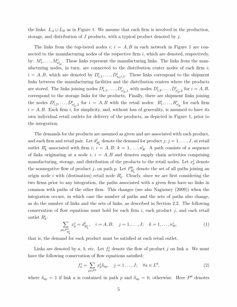
the links: LA ∪ LB as in Figure 1. We assume that each firm is involved in the production,

storage, and distribution of J products, with a typical product denoted by j.

The links from the top-tiered nodes i; i = A, B in each network in Figure 1 are con-

nected to the manufacturing nodes of the respective firm i, which are denoted, respectively,

by: M i1, . . . ,M

ini

M. These links represent the manufacturing links. The links from the man-

ufacturing nodes, in turn, are connected to the distribution center nodes of each firm i;

i = A, B, which are denoted by Di1,1, . . . , D

inD

i,1. These links correspond to the shipment

links between the manufacturing facilities and the distribution centers where the products

are stored. The links joining nodes Di1,1, . . . , D

ini

D,1 with nodes Di1,2, . . . , D

ini

D,2 for i = A, B,

correspond to the storage links for the products. Finally, there are shipment links joining

the nodes Di1,2, . . . , D

ini

D,2 for i = A, B with the retail nodes: Ri1, . . . , R

ini

Rfor each firm

i = A, B. Each firm i, for simplicity, and, without loss of generality, is assumed to have its

own individual retail outlets for delivery of the products, as depicted in Figure 1, prior to

the integration.

The demands for the products are assumed as given and are associated with each product,

and each firm and retail pair. Let djRi

kdenote the demand for product j; j = 1, . . . , J , at retail

outlet Rik associated with firm i; i = A, B; k = 1, . . . , ni

R. A path consists of a sequence

of links originating at a node i; i = A, B and denotes supply chain activities comprising

manufacturing, storage, and distribution of the products to the retail nodes. Let xjp denote

the nonnegative flow of product j, on path p. Let P 0Ri

kdenote the set of all paths joining an

origin node i with (destination) retail node Rik. Clearly, since we are first considering the

two firms prior to any integration, the paths associated with a given firm have no links in

common with paths of the other firm. This changes (see also Nagurney (2009)) when the

integration occurs, in which case the number of paths and the sets of paths also change,

as do the number of links and the sets of links, as described in Section 2.2. The following

conservation of flow equations must hold for each firm i, each product j, and each retail

outlet Rik: ∑

p∈P 0

Rik

xjp = dj

Rik, i = A, B; j = 1, . . . , J ; k = 1, . . . , ni

R, (1)

that is, the demand for each product must be satisfied at each retail outlet.

Links are denoted by a, b, etc. Let f ja denote the flow of product j on link a. We must

have the following conservation of flow equations satisfied:

f ja =

∑p∈P 0

xjpδap, j = 1 . . . , J ; ∀a ∈ L0, (2)

where δap = 1 if link a is contained in path p and δap = 0, otherwise. Here P 0 denotes

5

the set of all paths in Figure 1, that is, P 0 = ∪i=A,B;k=1,...,niRP 0

Rik. The path flows must be

nonnegative, that is,

xjp ≥ 0, j = 1, . . . , J ; ∀p ∈ P 0. (3)

We group the path flows into the vector x.

Note that the different products flow on the supply chain networks depicted in Figure 1

and share resources with one another. To capture the costs, we proceed as follows. There

is a total cost associated with each product j; j = 1, . . . , J , and each link (cf. Figure 1)

of the network corresponding to each firm i; i = A, B. We denote the total cost on a link

a associated with product j by cja. The total cost of a link associated with a product, be

it a manufacturing link, a shipment/distribution link, or a storage link is assumed to be

a function of the flow of all the products on the link; see, for example, Dafermos (1973).

Hence, we have that

cja = cj

a(f1a , . . . , fJ

a ), j = 1, . . . , J ; ∀a ∈ L0. (4)

The top tier links in Figure 1 have total cost functions associated with them that capture

the manufacturing costs of the products; the second tier links have multiproduct total cost

functions associated with them that correspond to the total costs associated with the sub-

sequent distribution/shipment to the storage facilities, and the third tier links, since they

are the storage links, have associated with them multiproduct total cost functions that cor-

respond to storage. Finally, the bottom-tiered links, since they correspond to the shipment

links to the retailers, have total cost functions associated with them that capture the costs

of shipment of the products.

We assume that the total cost function for each product on each link is convex, continu-

ously differentiable, and has a bounded third order partial derivative. Since the firms’ supply

chain networks, pre-integration, have no links in common (cf. Figure 1), their individual cost

minimization problems can be formulated jointly as follows:

MinimizeJ∑

j=1

∑a∈L0

cja(f

1a , . . . , fJ

a ) (5)

subject to: constraints (1) – (3) and the following capacity constraints:

J∑j=1

αjfja ≤ ua, ∀a ∈ L0. (6)

The term αj denotes the volume taken up by product j, whereas ua denotes the nonnegative

capacity of link a.

6

Observe that this problem is, as is well-known in the transportation literature (cf. Beck-

mann, McGuire, and Winsten (1956), Dafermos and Sparrow (1969), and Dafermos (1973)),

a system-optimization problem but in capacitated form. Under the above imposed assump-

tions, the optimization problem is a convex optimization problem. If we further assume that

the feasible set underlying the problem represented by the constraints (1) – (3) and (6) is

non-empty, then it follows from the standard theory of nonlinear programming (cf. Bazaraa,

Sherali, and Shetty (1993)) that an optimal solution exists.

Let K0 denote the set where K0 ≡ {f |∃x such that (1) − (3) and (6) hold}, where f is

the vector of link flows. We assume that the feasible set K0 is non-empty. We associate

the Lagrange multiplier βa with constraint (6) for each a ∈ L0. We denote the associated

optimal Lagrange multiplier by β∗a. This term may be interpreted as the price or value of

an additional unit of capacity on link a; it is also sometimes refered to as the shadow price.

We now provide the variational inequality formulation of the problem. For convenience, and

since we are considering Case 0, we denote the solution of variational inequality (7) below

as (f 0∗, β0∗) and we refer to the corresponding vectors of variables with superscripts of 0.

Theorem 1

The vector of link flows f 0∗ ∈ K0 is an optimal solution to the pre-integration problem if and

only if it satisfies the following variational inequality problem with the vector of nonnegative

Lagrange multipliers β0∗:

J∑j=1

J∑l=1

∑a∈L0

[∂cl

a(f1∗a , . . . , fJ∗

a )

∂f ja

+ αjβ∗a]× [f j

a − f j∗a ] +

∑a∈L0

[ua −J∑

j=1

αjfj∗a ]× [βa − β∗a] ≥ 0,

∀f 0 ∈ K0,∀β0 ≥ 0. (7)

Proof: See Bertsekas and Tsitsiklis (1989) and Nagurney (1999).

2.2 The Post-Integration Multiproduct Supply Chain Network Model

We now formulate the post-integration case, referred to as Case 1. Figure 2 depicts the

post-integration supply chain network topology. Note that there is now a supersource node

0 which represents the integration of the firms in terms of their supply chain networks with

additional links joining node 0 to nodes A and B, respectively.

As in the pre-integration case, the post-integration optimization problem is also con-

cerned with total cost minimization. Specifically, we retain the nodes and links associated

with the network depicted in Figure 1 but now we add the additional links connecting the

7

RA1

m · · · mRAnA

RRB

1m · · · mRB

nBR

?

HH

HH

HHj?

��

��

���

PPPPPPPPPq?

HH

HH

HHj

���������) ?

��

��

���

DA1,2

m · · · mDAnA

D,2 DB1,2

m · · · mDBnB

D,2

? ? ? ?

DA1,1

m · · · mDAnA

D,1 DB1,1

m · · · mDBnB

D,1

?

HH

HH

HHj?

��

��

���

PPPPPPPPPq?

HH

HH

HHj

���������) ?

��

��

���

MA1

m · · · mMAnA

MMB

1m · · · mMB

nBM

��

�

@@

@R

��

�

@@

@R

mA mB�

��

��

����

HH

HH

HH

HHj

m0Firm A Firm B

Figure 2: Supply Chain Network after Firms A and B Merge

manufacturing facilities of each firm and the distribution centers of the other firm as well as

the links connecting the distribution centersof each firm and the retail outlets of the other

firm. We refer to the network in Figure 2, underlying this integration, as G1 = [N1, L1]

where N1 ≡ N0∪ node 0 and L1 ≡ L0∪ the additional links as in Figure 2. We associate

total cost functions as in (4) with the new links, for each product j. Note that if the total

cost functions associated with the integration/merger links connecting node 0 to node A and

node 0 to node B are set equal to zero, this means that the supply chain integration is costless

in terms of the supply chain integration/merger of the two firms. Of course, non-zero total

cost functions associated with these links may be utilized to also capture the risk associated

with the integration. We will explore such issues numerically in Section 4.

A path p now (cf. Figure 2) originates at the node 0 and is destined for one of the bottom

retail nodes. Let xjp, in the post-integrated network configuration given in Figure 2, denote

the flow of product j on path p joining (origin) node 0 with a (destination) retail node.

Then, the following conservation of flow equations must hold:

∑p∈P 1

Rik

xjp = dj

Rik, i = A, B; j = 1, . . . , J ; k = 1, . . . , ni

R, (8)

where P 1Ri

kdenotes the set of paths connecting node 0 with retail node Ri

k in Figure 2. Due to

the integration, the retail outlets can obtain each product j from any manufacturing facility,

and any distributor. The set of paths P 1 ≡ ∪i=A,B;k=1,...,niRP 1

Rik.

In addition, as before, let f ja denote the flow of product j on link a. Hence, we must also

8

have the following conservation of flow equations satisfied:

f ja =

∑p∈P 1

xjpδap, j = 1, . . . , J ; ∀a ∈ L1. (9)

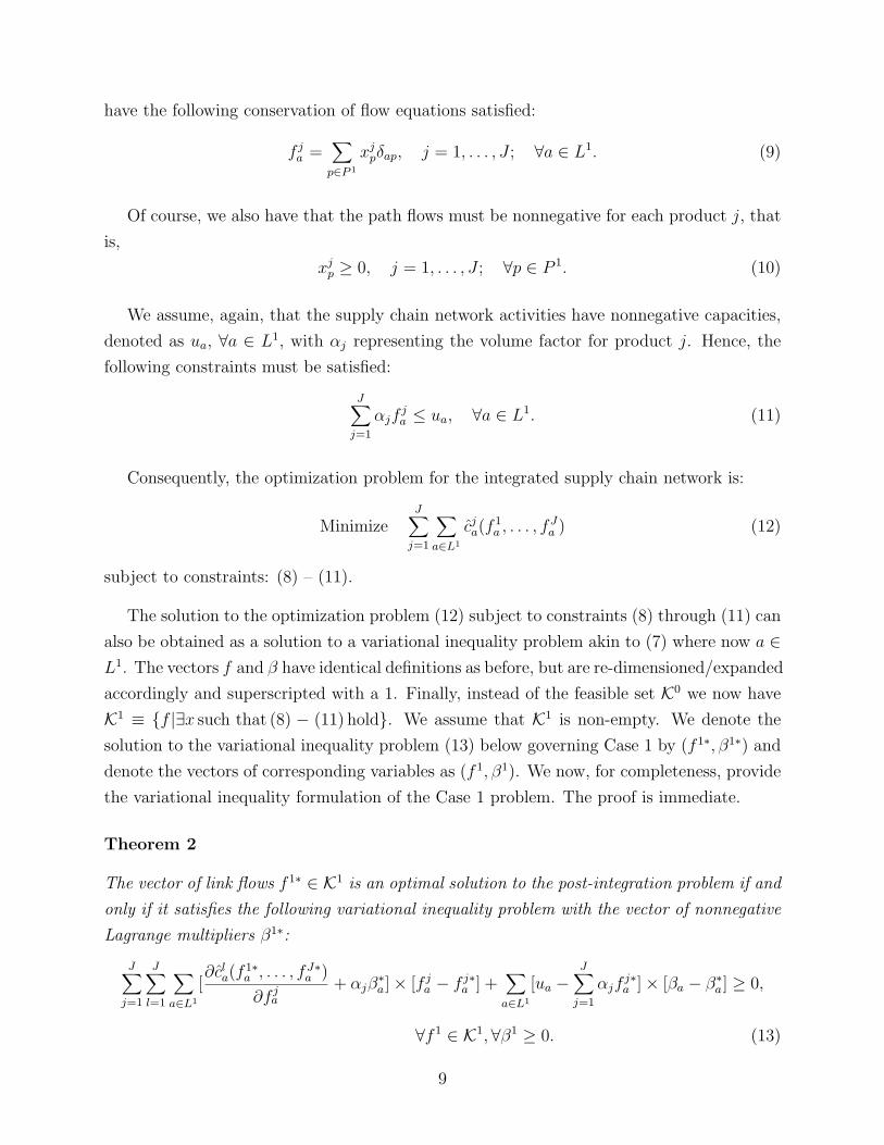
Of course, we also have that the path flows must be nonnegative for each product j, that

is,

xjp ≥ 0, j = 1, . . . , J ; ∀p ∈ P 1. (10)

We assume, again, that the supply chain network activities have nonnegative capacities,

denoted as ua, ∀a ∈ L1, with αj representing the volume factor for product j. Hence, the

following constraints must be satisfied:

J∑j=1

αjfja ≤ ua, ∀a ∈ L1. (11)

Consequently, the optimization problem for the integrated supply chain network is:

MinimizeJ∑

j=1

∑a∈L1

cja(f

1a , . . . , fJ

a ) (12)

subject to constraints: (8) – (11).

The solution to the optimization problem (12) subject to constraints (8) through (11) can

also be obtained as a solution to a variational inequality problem akin to (7) where now a ∈L1. The vectors f and β have identical definitions as before, but are re-dimensioned/expanded

accordingly and superscripted with a 1. Finally, instead of the feasible set K0 we now have

K1 ≡ {f |∃x such that (8) − (11) hold}. We assume that K1 is non-empty. We denote the

solution to the variational inequality problem (13) below governing Case 1 by (f 1∗, β1∗) and

denote the vectors of corresponding variables as (f 1, β1). We now, for completeness, provide

the variational inequality formulation of the Case 1 problem. The proof is immediate.

Theorem 2

The vector of link flows f 1∗ ∈ K1 is an optimal solution to the post-integration problem if and

only if it satisfies the following variational inequality problem with the vector of nonnegative

Lagrange multipliers β1∗:

J∑j=1

J∑l=1

∑a∈L1

[∂cl

a(f1∗a , . . . , fJ∗

a )

∂f ja

+ αjβ∗a]× [f j

a − f j∗a ] +

∑a∈L1

[ua −J∑

j=1

αjfj∗a ]× [βa − β∗a] ≥ 0,

∀f 1 ∈ K1,∀β1 ≥ 0. (13)

9

We let TC0 denote the total cost,∑J

j=1

∑a∈L0 cj

a(f1a , . . . , fJ

a ), evaluated under the solution

f 0∗ to (7) and we let TC1,∑J

j=1

∑a∈L1 cj

a(f1a , . . . , fJ

a ) denote the total cost evaluated under

the solution f 1∗ to (13). Due to the similarity of variational inequalities (7) and (13) the same

computational procedure can be utilized to compute the solutions. Indeed, we utilize the

variational inequality formulations of the respective pre- and post-integration supply chain

network problems since we can then exploit the simplicity of the underlying feasible sets

K0 and K1 which include constraints with a network structure identical to that underlying

multimodal system-optimized transportation network problems.

It is worthwhile to distinguish the multiproduct supply chain network models developed

above from the single product models in Nagurney (2009). First, we note that the total cost

functions in the objective functions (5) and (12) are not separable as they were, respectively,

in the single product models in Nagurney (2009). In addition, since we are dealing now with

multiple products, which can be of different physical dimensions, the corresponding capacity

constraints (cf. (6) and (11)) are also more complex than was the case for their single

product counterparts. We also emphasize that the above multiproduct framework contains,

as a special case, the merger of firms that produce (pre-merger) distinct products, which is

captured by assigning a demand of zero to those products at the respective demand markets.

Of course, in such a case, the total cost functions would also be adapted accordingly.

Finally, the multiproduct models developed in this paper allow for non-zero total costs

associated with the top-most merger links (cf. Figure 2), which join node 0 to nodes A and B.

In Nagurney (2009) it was assume that the corresponding total costs, in the single product

case, were zero. Of course, it would also be interesting to explore the issue of “retooling” a

manufacturing facility, post-merger, for it to be able to produce the other firm’s product(s)

in its original manufacturing facilities.

3. Quantifying Synergy Associated with Multiproduct Supply Chain Network

Integration

We measure the synergy by analyzing the total costs prior to and post the supply chain

network integration (cf. Eccles et al. (1999) and Nagurney (2009)). For example, the synergy

based on total costs and proposed by Nagurney (2009), but now in a multiproduct context,

which we denote here by STC , can be calculated as the percentage difference between the

total cost pre vs the total cost post the integration:

STC ≡ [TC0 − TC1

TC0]× 100%. (14)

From (14), one can see that the lower the total cost TC1, the higher the synergy associated

10

with the supply chain network integration. Of course, in specific firm operations one may

wish to evaluate the integration of supply chain networks with only a subset of the links

joining the original two supply chain networks. In that case, Figure 2 would be modified

accordingly and the synergy as in (14) computed with TC1 corresponding to that new supply

chain network topology.

We now provide a theorem which shows that if the total costs associated with the inte-

gration of the supply chain networks of the two firms are identically equal to zero, then the

associated synergy can never be negative.

Theorem 3

If the total cost functions associated with the integration/merger links from node 0 to nodes

A and B for each product are identically equal to zero, then the associated synergy, STC, can

never be negative.

Proof: We first note that the pre-integration supply chain optimization problem can be

defined over the same expanded network as in Figure 2 but with the cross-shipment links

extracted and with the paths defined from node 0 to the retail nodes. In addition, the

total costs from node 0 to nodes A and B must all be equal to zero. Clearly, the total cost

minimization solution to this problem yields the same total cost value as obtained for TC0.

We must now show that TC0 − TC1 ≥ 0.

Assume not, that is, that TC0−TC1 < 0, then, clearly, we have not obtained an optimal

solution to the post-integration problem, since, the new links need not be used, which would

imply that TC0 = TC1, which is a contradiction. 2

Another interpretation of this theorem is that, in the system-optimization context (as-

suming that the total cost functions remain the same as do the demands), the addition of

new links can never make the total cost increase; this is in contrast to what may occur in

the context of user-optimized networks, where the addition of a new link may make everyone

worse-off in terms of user cost. This is the well-known Braess paradox (1968); see, also,

Braess et al. (2005).

4. Numerical Examples

In this Section, we present numerical examples for which we compute the solutions to the

supply chains both pre and post the integration, along with the associated total costs and

synergies as defined in Section 3. The examples were solved using the modified projection

11

method (see, e.g., Korpelevich (1977) and Nagurney (2009)) embedded with the equilibration

algorithm (cf. Dafermos and Sparrow (1969) and Nagurney (1984)). The modified projection

method is guaranteed to converge if the function that enters the variational inequality is

monotone and Lipschitz continuous (provided that a solution exists). Both these assumptions

are satisfied under the conditions imposed on the multiproduct total cost functions in Section

2 as well as by the total cost functions underlying the numerical examples below. Since

we also assume that the feasible sets are non-empty, we are guaranteed that the modified

projection method will converge to a solution of variational inequalities (7) and (13).

We implemented the computational procedure in FORTRAN and utilized a Unix sys-

tem at the University of Massachusetts Amherst for the computations. The algorithm was

considered to have converged when the absolute value of the difference between the com-

puted values of the variables (the link flows; respectively, the Lagrange multipliers) at two

successive iterations differed by no more than 10−5. In order to fully exploit the under-

lying network structure, we first converted the multiproduct supply chain networks, into

single-product “extended” ones as discussed in Dafermos (1973) for multimodal/multiclass

traffic networks. The link capacity constraints, which do not explicitly appear in the original

traffic network models, were adapted accordingly. The modified projecion method yielded

subproblems, at each iteration, in flow variables and in price variables. The former were

computed using the equilibration algorithm of Dafermos and Sparrow (1969) and the latter

were computed explicitly and in closed form.

For all the numerical examples, we assumed that each firm i; i = A, B, was involved

in the production, storage, and distribution of two products, and each firm had, prior to

the integration/merger, two manufacturing plants, one distribution center, and supplied the

products to two retail outlets.

After the integration of the two firms’ supply chain networks, each retailer was indifferent

as to which firm supplied the products and the integrated/merged firms could store the

products at any of the two distribution centers and could supply any of the four retailers.

Figure 3 depicts the pre-integration supply chain network(s), whereas Figure 4 depicts the

post-integration supply chain network for the numerical examples.

For all the examples, we assumed that the pre-integration total cost functions and the

post-integration total cost functions were nonlinear (quadratic), of the form:

cja(f

1a , f2

a ) =2∑

l=1

gjla f j

af la + hj

afja , ∀a ∈ L0,∀a ∈ L1; j = 1, 2, (15)

with convexity of the total cost functions being satisfied (except, where noted, for the top-

12

RA1

m mRA2 RB

1m mRB

2

��

�

@@

@R

@@

@R

��

�

DA1,2

m mDB1,2

? ?

DA1,1

m mDB1,1

@@

@R

��

�

@@

@R

��

�

MA1

m mMA2 MB

1m mMB

2

��

�

@@

@R

��

�

@@

@R

mA mBFirm A Firm B

Figure 3: Pre-Integration Supply Chain Network Topology for the Numerical Examples

most merger links from node 0).

13

RA1

m mRA2 RB

1m mRB

2

��

�

@@

@R

XXXXXXXXXXXXz

@@

@R

��

�

������������9

DA1,2

m mDB1,2

? ?

DA1,1

m mDB1,1

@@

@R

��

�

XXXXXXXXXXXXz

@@

@R

������������9

��

�

MA1

m mMA2 MB

1m mMB

2

��

�

@@

@R

��

�

@@

@R

mA mB�

��

��

����

HH

HH

HH

HHj

m0Firm A Firm B

Figure 4: Post-Integration Supply Chain Network Topology for the Examples

Example 1

Example 1 served as the baseline for our computations. The Example 1 data are now

described. The pre and post-integration total cost functions for products 1 and 2 are listed

in Table 1. The links post-integration that join the node 0 with nodes A and B had associated

total costs equal to zero for each product j = 1, 2, for Examples 1 through 3. The demands

at the retail outlets for Firm A and Firm B were set to 5 for each product. Hence, djRi

k= 5

for i = A, B; j = 1, 2, and k = 1, 2. The capacity on each link was set to 25 both pre and

post integration, so that: ua = 25 for all links a ∈ L0; a ∈ L1. The weights: αj = 1 were set

to 1 for both products j = 1, 2, both pre and post-integration; thus, we assumed that the

products are equal in volume.

The pre-integration optimal solutions for the product flows for each product for Examples

1 through 3 are given in Table 2. We note that Example 1, pre-integration, was used as the

basis from which variants post-integration were constructed, yielding Examples 2 and 3, as

described below.

The post-integration optimal solutions are reported in Table 3 for product 1 and in Table

4 for product 2.

Since none of the link flow capacities were reached, either pre- or post-integration, the

vectors β0∗ and β1∗ had all their components equal to zero. The total cost, pre-merger,

TC0 = 5, 702.58. The total cost, post-merger, TC1 = 4, 240.86. Please also refer to Table 5

for the total cost and synergy values for this example as well as for the next two examples.

14

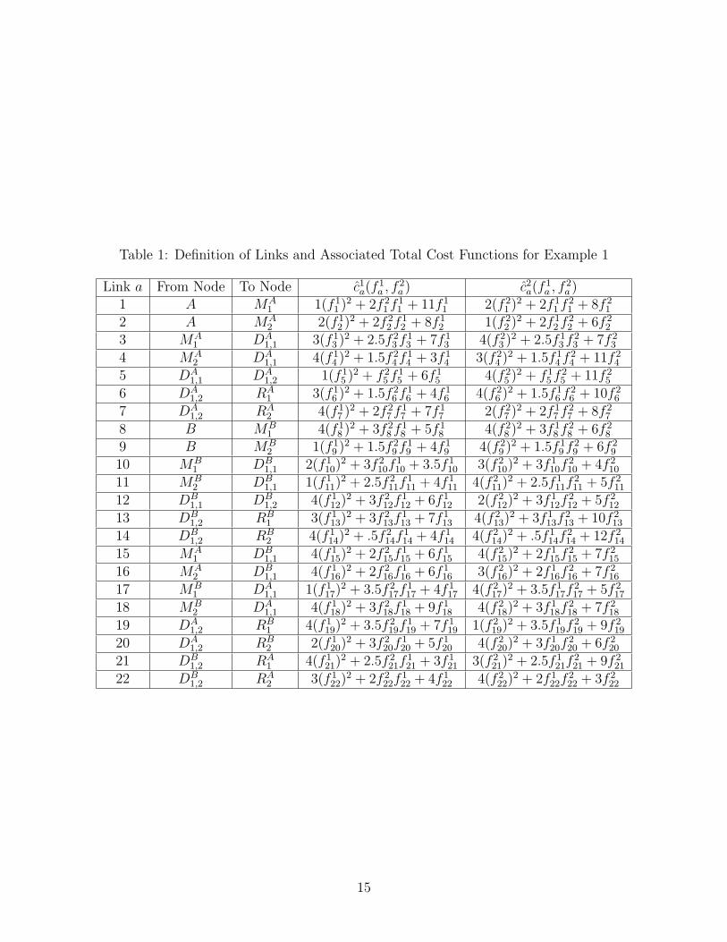
Table 1: Definition of Links and Associated Total Cost Functions for Example 1

Link a From Node To Node c1a(f

1a , f2

a ) c2a(f

1a , f2

a )1 A MA

1 1(f 11 )2 + 2f 2

1 f 11 + 11f 1

1 2(f 21 )2 + 2f 1

1 f 21 + 8f 2

1

2 A MA2 2(f 1

2 )2 + 2f 22 f 1

2 + 8f 12 1(f 2

2 )2 + 2f 12 f 2

2 + 6f 22

3 MA1 DA

1,1 3(f 13 )2 + 2.5f 2

3 f 13 + 7f 1

3 4(f 23 )2 + 2.5f 1

3 f 23 + 7f 2

3

4 MA2 DA

1,1 4(f 14 )2 + 1.5f 2

4 f 14 + 3f 1

4 3(f 24 )2 + 1.5f 1

4 f 24 + 11f 2

4

5 DA1,1 DA

1,2 1(f 15 )2 + f 2

5 f 15 + 6f 1

5 4(f 25 )2 + f 1

5 f 25 + 11f 2

5

6 DA1,2 RA

1 3(f 16 )2 + 1.5f 2

6 f 16 + 4f 1

6 4(f 26 )2 + 1.5f 1

6 f 26 + 10f 2

6

7 DA1,2 RA

2 4(f 17 )2 + 2f 2

7 f 17 + 7f 1

7 2(f 27 )2 + 2f 1

7 f 27 + 8f 2

7

8 B MB1 4(f 1

8 )2 + 3f 28 f 1

8 + 5f 18 4(f 2

8 )2 + 3f 18 f 2

8 + 6f 28

9 B MB2 1(f 1

9 )2 + 1.5f 29 f 1

9 + 4f 19 4(f 2

9 )2 + 1.5f 19 f 2

9 + 6f 29

10 MB1 DB

1,1 2(f 110)

2 + 3f 210f

110 + 3.5f 1

10 3(f 210)

2 + 3f 110f

210 + 4f 2

10

11 MB2 DB

1,1 1(f 111)

2 + 2.5f 211f

111 + 4f 1

11 4(f 211)

2 + 2.5f 111f

211 + 5f 2

11

12 DB1,1 DB

1,2 4(f 112)

2 + 3f 212f

112 + 6f 1

12 2(f 212)

2 + 3f 112f

212 + 5f 2

12

13 DB1,2 RB

1 3(f 113)

2 + 3f 213f

113 + 7f 1

13 4(f 213)

2 + 3f 113f

213 + 10f 2

13

14 DB1,2 RB

2 4(f 114)

2 + .5f 214f

114 + 4f 1

14 4(f 214)

2 + .5f 114f

214 + 12f 2

14

15 MA1 DB

1,1 4(f 115)

2 + 2f 215f

115 + 6f 1

15 4(f 215)

2 + 2f 115f

215 + 7f 2

15

16 MA2 DB

1,1 4(f 116)

2 + 2f 216f

116 + 6f 1

16 3(f 216)

2 + 2f 116f

216 + 7f 2

16

17 MB1 DA

1,1 1(f 117)

2 + 3.5f 217f

117 + 4f 1

17 4(f 217)

2 + 3.5f 117f

217 + 5f 2

17

18 MB2 DA

1,1 4(f 118)

2 + 3f 218f

118 + 9f 1

18 4(f 218)

2 + 3f 118f

218 + 7f 2

18

19 DA1,2 RB

1 4(f 119)

2 + 3.5f 219f

119 + 7f 1

19 1(f 219)

2 + 3.5f 119f

219 + 9f 2

19

20 DA1,2 RB

2 2(f 120)

2 + 3f 220f

120 + 5f 1

20 4(f 220)

2 + 3f 120f

220 + 6f 2

20

21 DB1,2 RA

1 4(f 121)

2 + 2.5f 221f

121 + 3f 1

21 3(f 221)

2 + 2.5f 121f

221 + 9f 2

21

22 DB1,2 RA

2 3(f 122)

2 + 2f 222f

122 + 4f 1

22 4(f 222)

2 + 2f 122f

222 + 3f 2

22

15

Table 2: Pre-Integration Optimal Product Flow Solutions to Examples 1 Through 3Link a From Node To Node f 1∗

a f 2∗a

1 A MA1 8.50 .80

2 A MA2 1.50 9.20

3 MA1 DA

1,1 8.50 .80

4 MA2 DA

1,1 1.50 9.20

5 DA1,1 DA

1,2 10.00 10.00

6 DA1,2 RA

1 5.00 5.00

7 DA1,2 RA

2 5.00 5.00

8 B MB1 0.00 8.03

9 B MB2 10.00 1.97

10 MB1 DB

1,1 0.00 8.03

11 MB2 DB

1,1 10.00 1.97

12 DB1,1 DB

1,2 10.00 10.00

13 DB1,2 RB

1 5.00 5.00

14 DB1,2 RB

2 5.00 5.00

The synergy STC for the supply chain network integration for Example 1 was equal to

25.63%.

It is interesting to note that, since the distribution center associated with the original Firm

A has total storage costs that are lower for product 1, whereas Firm B’s distribution center

has lower costs associated with the storage of product 2, that Firm A’s original distribution

center, after the integration/merger, stores the majority of the volume of product 1, while

the majority of the volume of product 2 is stored, post-integration, at Firm B’s original

distribution center. It is also interesting to note that, post-integration, the majority of the

production of product 1 takes place in Firm B’s original manufacturing plants, whereas the

converse holds true for product 2. This example, hence, vividly illustrates the types of supply

chain cost gains that can be achieved in the integration of multiproduct supply chains.

16

Table 3: Post-Integration Optimal Flow Solutions to the Examples for Product 1

Link a From Node To Node Ex. 1 f 1∗a Ex. 2 f 1∗

a Ex. 3 f 1∗a

1 A MA1 5.94 0.76 5.36

2 A MA2 0.53 0.00 1.98

3 MA1 DA

1,1 5.94 0.00 5.36

4 MA2 DA

1,1 0.53 0.00 1.98

5 DA1,1 DA

1,2 18.27 19.24 17.34

6 DA1,2 RA

1 5.00 5.00 5.00

7 DA1,2 RA

2 3.27 4.24 4.27

8 B MB1 6.25 1.67 5.00

9 B MB2 7.29 17.57 7.66

10 MB1 DB

1,1 0.00 0.00 0.00

11 MB2 DB

1,1 1.73 0.00 2.66

12 DB1,1 DB

1,2 1.73 0.76 2.66

13 DB1,2 RB

1 0.00 0.00 0.00

14 DB1,2 RB

2 0.00 0.00 1.93

15 MA1 DB

1,1 0.00 0.76 0.00

16 MA2 DB

1,1 0.00 0.00 0.00

17 MB1 DA

1,1 6.25 1.67 5.00

18 MB2 DA

1,1 5.55 17.57 5.00

19 DA1,2 RB

1 5.00 5.00 5.00

20 DA1,2 RB

2 5.00 5.00 3.07

21 DB1,2 RA

1 0.00 0.00 0.00

22 DB1,2 RA

2 1.73 0.76 0.73

17

Table 4: Post-Integration Optimal Flow Solutions to the Examples for Product 2

Link a From Node To Node Ex. 1 f 2∗a Ex. 2 f 2∗

a Ex. 3 f 2∗a

1 A MA1 3.44 4.66 5.00

2 A MA2 11.81 11.88 8.74

3 MA1 DA

1,1 0.00 0.88 0.00

4 MA2 DA

1,1 4.91 0.48 3.74

5 DA1,1 DA

1,2 4.91 4.82 3.74

6 DA1,2 RA

1 1.52 0.00 0.61

7 DA1,2 RA

2 2.58 0.00 1.20

8 B MB1 2.34 3.46 3.58

9 B MB2 2.42 0.00 2.68

10 MB1 DB

1,1 2.34 0.00 3.58

11 MB2 DB

1,1 2.42 0.00 2.68

12 DB1,1 DB

1,2 15.09 15.18 16.26

13 DB1,2 RB

1 4.88 2.72 5.00

14 DB1,2 RB

2 4.30 2.46 3.07

15 MA1 DB

1,1 3.44 3.78 5.00

16 MA2 DB

1,1 6.89 11.40 5.00

17 MB1 DA

1,1 0.00 3.46 0.00

18 MB2 DA

1,1 0.00 0.00 0.00

19 DA1,2 RB

1 0.12 2.28 0.00

20 DA1,2 RB

2 0.70 2.54 1.93

21 DB1,2 RA

1 3.48 5.00 4.39

22 DB1,2 RA

2 2.42 5.00 3.80

18

Example 2

Example 2 was constructed from Example 1 but with the following modifications. We now

considered an idealized situation in which we assumed that the total costs associated with

the new integration links; see Table 1 (links 15 through 22) for each product were identically

equal to zero.

Post-integration, the optimal flow for each product, for each firm, has now changed; see

Table 3 and Table 4. It is interesting to note that now the second manufacturing plant

associated with the original Firm B produces the majority of product 1 but the majority

of product 1 is still stored at the original distribution center of Firm A. Indeed, the zero

costs associated with distribution between the original supply chain networks lead to further

synergies as compared to those obtained for Example 1.

Since, again, none of the link flow capacities were reached, either pre- or post-integration,

the vectors β0∗ and β1∗ had all their components equal to zero. The total cost, post-merger,

TC1 = 2, 570.27. The synergy STC for the supply chain network integration for Example

2 was equal to 54.93%. Observe that this obtained synergy is, in a sense, the maximum

possible for this example since the total costs for both products on all the new links are all

equal to zero.

Example 3

Example 3 was constructed from Example 2 but with the following modifications. We now

assumed that the capacities associated with the links that had zero costs between the two

original firms had their capacities reduced from 25 to 5. The computed optimal flow solutions

are given in Table 3 for product 1 and in Table 4 for product 2.

We now also provide the computed vector of Lagrange multipliers β1∗. All terms were

equal to zero except those for links 15 through 20 since the sum of the corresponding product

flows on each of these links was equal to the imposed capacity of 5. In particular, we now

had: β∗15 = 40.82, β∗16 = 59.79, β∗17 = 14.35, β∗18 = 53.59, β∗19 = 79.95, and β∗20 = 68.39.

The total cost, post-merger, was now TC1 = 3, 452.34. The synergy STC for the supply

chain network integration for Example 3 was equal to 39.46%. Hence, even with substantially

lower capacities on the new links, given the zero costs, the synergy associated with the supply

chain network integration in Example 3 was quite high, although not as high as obtained in

Example 2.

Firm B’s original distribution center now stores more of product 1 and 2 than it did

19

Table 5: Total Costs and Synergy Values for the Examples

Measure Example 1 Example 2 Example 3Pre-Integration TC0 5,702.58 5,702.58 5,702.58Post-Integration TC1 4,240.86 2,570.27 3,452.34

Synergy Calculations STC 25.63% 54.93% 39.46%

in Example 2 (post-integration). Also, because of capacity reductions associated with the

cross-shipment links there is a notable reduction in the volume of shipment of product 1

from the second manufacturing plant of Firm B to Firm A’s original distribution center and

in the shipment of product 2 from Firm A’s original second manufacturing plant to Firm B’s

original distribution center.

Additional Computations/Examples

We then proceeded to ask the following question: assuming that the links, post-merger,

joining node 0 to nodes A and B no longer had zero associated total cost for each product

but, rather, reflected a cost associated with merging the two firms. We further assumed that

the cost (cf. (15)) was linear and of the specific form given by

cja = hj

afja = hf j

a , j = 1, 2

for the upper-most links (cf. Figure 4). Hence, we assumed that all the hja terms were

identical and equal to an h. At what value would the synergy then for Examples 1, 2, and

3 become negative? Through computational experiments we were able to determine these

values. In the case of Example 1, if h = 36.52, then the synergy value would be approximately

equal to zero since the new total cost would be approximately equal to TC0 = 5, 702.58.

For any value larger than the above h, one would obtain negative synergy. This has clear

implications for mergers in terms of supply chain network integration and demonstrates that

the total costs associated with the integration/merger itself have to be carefully weighed

against the cost benefits associated with the integrated supply chain activities. In the case

of Example 2, the h value was approximately equal to 78.3. A higher value than this h for

each such merger link would result in the total cost exceeding TC0 and, hence, negative

synergy would result.

Finally, for completeness, we also determined the corresponding h in the case of Example

3 and found the value to be h = 78.3, as in Example 2.

20

5. Summary and Conclusions

In this paper, we developed multiproduct supply chain network models, which allow one

to evaluate the total costs associated with manufacturing/production, storage, and distribu-

tion of firms’ supply chains both pre and post-integration. Such horizontal integrations can

take place, for example, in the context of mergers and acquisitions, an activity which has

garnered much interest and momentum recently. The model(s) utilize a system-optimization

perspective and allow for explicit upper bounds on the various links associated with man-

ufacturing, storage, and distribution. The models are formulated and solved as variational

inequality problems.

In addition, we utilized a proposed multiproduct synergy measure to identify the po-

tential cost gains associated with such horizontal supply chain network integrations. We

proved that, in the case of zero “merging” costs, that the associated synergy can never be

negative. We computed solutions to several numerical examples for which we determine the

optimal product flows and Lagrange multipliers/shadow prices associated with the capacity

constraints both before and after the integration. The computational approach allows one to

explore many issues regarding supply chain network integration and to effectively ascertain

the synergies prior to any implementation of a potential merger. In addition, we determined,

computationally, for several examples, what identical linear costs would yield zero synergy,

with higher values resulting in negative synergy.

There are numerous questions that remain and that will be considered for future research.

It would be interesting to develop competitive variants of the models in a game theoretic

context and to also explore elastic demands. Also, this paper does consider the time di-

mension in that it models the supply chain networks before and after the proposed merger

and, hence, it considers two distinct point in time. For certain applications it may be useful

to have a more detailed time discretization with accompanying network structure. Finally,

it would be very interesting to explicitly incorporate the risks associated with supply chain

network integration within our framework.

Acknowledgments

This research was supported by the John F. Smith Memorial Fund at the Isenberg School

of Management. This support is gratefully acknowledged. The authors would also like to

thank Professor June Dong for helpful discussions.

The authors acknowledge the helpful comments and suggestions received during the re-

view process.

21

References

Bazaraa, M.S., Sherali, H.D., Shetty, C.M., 1993. Nonlinear programming: Theory and

algorithms (2nd edition). John Wiley & Sons, New York.

Beckmann, M.J., McGuire, C.B., Winsten, C.B., 1956. Studies in the economics of trans-

portation. Yale University Press, New Haven, Connecticut.

Bernard, A.B., Redding, S.J., Schott, P.K., 2006. Multi-product firms and product switch-

ing. Working paper, Dartmouth College, Hanover, New Hampshire;

http://mba.tuck.dartmouth.edu/pages/faculty/andrew.bernard/pswitch.pdf

Bertsekas, D.P., Tsitsiklis, J.N., 1989. Parallel and distributed computation - numerical

methods. Prentice Hall, Englewood Cliffs, New Jersey.

Braess, D., 1968. Uber ein paradoxon der verkehrsplanung. Unternehmenforschung 12,

258-268

Braess, D., Nagurney, A., Wakolbinger, T., 2005. On a paradox of traffic planning (transla-

tion of the Braess (1968) article from German). Transportation Science 39, 443-445.

Byrne, P.M. January 1, 2007. Unleashing supply chain value in mergers and acquisitions.

Logistics Management, 20-20.

Chang, P.C., 1988. A measure of the synergy in mergers under a competitive market for

corporate control. Atlantic Economic Journal 16, 59-62.

Cheng, T.C.E, Wu, Y.N., 2006. A multiproduct, multicriterion supply-demand network

equilibrium model. Operations Research 54, 544-554.

Dafermos, S.C., 1973. The traffic assignment problem for multiclass-user transportation

networks. Transportation Science 6, 73-87.

Dafermos, S.C., Sparrow, F.T., 1969. The traffic assignment problem for a general network.

Journal of Research of the National Bureau of Standards 73B, 91-118.

Davis, D.D., Wilson, B.J., 2006. Equilibrium price dispersion, mergers and synergies: An

experimental investigation of differentiated product competition. International Journal of

the Economics of Business 13, 169-194.

Dong, J., Zhang, D., Nagurney, A., 2004. A supply chain network equilibrium model with

random demands. European Journal of Operational Research 156, 194-212.

22

Eccles, R.G., Lanes, K.L., Wilson, T.C., 1999. Are you paying too much for that acquisition?

Harvard Business Review 77, 136-146.

Korpelevich, G.M., 1977. The extragradient method for finding saddle points and other

problems. Matekon 13, 35-49.

Langabeer, J., Seifert, D., 2003. Supply chain integration: The key to merger success. Supply

Chain Management Review 7, 58-64.

Min, H., Zhou, G., 2002. Supply chain modeling: Past, present and future. Computers and

Industrial Engineering 43, 231-249.

Nagurney, A., 1984. Computational comparisons of algorithms for general asymmetric traffic

equilibrium problems with fixed and elastic demands. Transportation Research B 18, 469-

485.

Nagurney, A., 1999. Network economics: a variational inequality approach (2nd edition).

Kluwer Academic Publishers, Dordrecht, The Netherlands.

Nagurney, A., 2006a. Supply chain network economics: Dynamics of prices, flows and profits.

Edward Elgar Publishing, Cheltenham, England.

Nagurney, A., 2006b. On the relationship between supply chain and transportation network

equilibria: A supernetwork equivalence with computations. Transportation Research E 42,

293-316.

Nagurney, A., 2009. A system-optimization perspective for supply chain integration: The

horizontal merger case. Transportation Research E 45, 1-15.

Soylu, A., Oru, C., Turkay, M., Fujita, K., Asakura, T., 2006. Synergy analysis of col-

laborative supply chain management in energy systems using multi-period MILP. European

Journal of Operational Research 174, 387-403.

Wang, Z., Zhang, F., Wang, Z., 2007. Research of return supply chain supernetwork model

based on variational inequalities. Proceedings of the IEEE International Conference on Au-

tomation and Logistics 25-30, Jinan, China.

Wong, G., October 10, 2007. After credit crisis, New forces drive deals. CNNMoney.com.

Xu, S., 2007. Supply chain synergy in mergers and acquisitions: Strategies, models and key

factors, PhD dissertation, University of Massachusetts, Amherst, Massachusetts.

23