Embed Size (px)
Citation preview
MPRAMunich Personal RePEc Archive
Multiproduct Pricing Made Simple
Mark Armstrong and John Vickers
Department of Economics, University of Oxford
8. January 2016
Online at https://mpra.ub.uni-muenchen.de/68717/MPRA Paper No. 68717, posted 8. January 2016 14:27 UTC
Multiproduct Pricing Made Simple
Mark Armstrong and John Vickers∗
January 2016
Abstract
We study pricing by multiproduct firms in the context of unregulated monopoly,regulated monopoly and Cournot oligopoly. Using the concept of consumer surplusas a function of quantities (rather than prices), we present simple formulas for opti-mal prices and show that Cournot equilibrium exists and corresponds to a Ramseyoptimum. We then present a tractable class of demand systems that involve a general-ized form of homothetic preferences. As well as standard homothetic preferences, thisclass includes linear and logit demand. Within the class, profit-maximizing quantitiesare proportional to effi cient quantities. We discuss cost-passthrough, including caseswhere optimal prices do not depend on other products’ costs. Finally, we discussoptimal monopoly regulation when the firm has private information about its vectorof marginal costs, and show that if the probability distribution over costs satisfies anindependence property, then optimal regulation leaves relative price decisions to thefirm.
Keywords: Multiproduct pricing, homothetic preferences, Cournot oligopoly, monopolyregulation, Ramsey pricing, cost passthrough, multidimensional screening.
JEL Classification: D42, D43, D82, L12, L13, L51.
1 Introduction
The theory of multiproduct pricing is a large and diverse subject. Unlike the single-product
case, a multiproduct firm must decide about the structure of its relative prices as well as
its overall price level. Classical questions include the characterization of optimal pricing
by a multiproduct monopolist seeking to maximize profit– or, as with Ramsey pricing, the
most effi cient way to generate a specified level of profit– when its choice for one price must
∗Both authors at All Souls College and the Department of Economics, University of Oxford. Weare grateful to Konrad Stahl (who discussed an early version this paper at the University of Mannheimworkshop on “Multiproduct firms in industrial organization and international trade”, 23-24 October, 2015)and to Jonas Müller-Gastell for helpful comments.
1

take into account its impact on demand for other products. Additional complexities arise
in oligopoly, when a multiproduct firm needs to choose prices to reflect both intra-firm
substitution (or complementarity) features and inter-firm interactions. Optimal regulation
of a multiproduct firm with private information about its costs, say, must take into account
not just its likely average cost across all products but its pattern of relative costs.
In this paper we show how these issues can be illuminated by studying consumer prefer-
ences in terms of consumer surplus considered as a function of quantities (rather than the
more familiar function of prices).1 In section 2 we show how profit-maximizing and other
Ramsey prices, as well as prices in symmetric Cournot equilibrium, can be expressed as a
markup over marginal costs proportional to the derivative of this surplus function. In par-
ticular, a product’s optimal price is below marginal cost when consumer surplus decreases
with the supply of this product. We also show how a Cournot equilibrium corresponds
to an appropriate Ramsey optimum, and vice versa, which enables us to construct and
demonstrate existence of Cournot equilibrium in many cases.
A well-known feature of Ramsey pricing is that when required departures of optimal
quantities from effi cient quantities are small, then optimal quantities are approximately
proportional to the effi cient quantities. Thus, a reasonable rule of thumb is often to scale
down quantities equiproportionately relative to effi cient quantities, rather than to increase
prices equiproportionately above marginal cost. For larger departures of prices from costs,
though, optimal quantities are generally not proportional to effi cient quantities. In section
3, we specialise the demand system so that consumer surplus is a homothetic function
of quantities, which implies that relative quantities (or relative price-cost markups) do
not depend on the weight placed on profit in the Ramsey objective. As shown in section
3.2, this is quite a flexible class of demand systems (much broader than the class where
consumer surplus is homothetic in prices), and as well as the obvious case of gross utility
being homothetic in quantities it includes linear and logit demands.
In section 3.3, we show that this property, together with assuming constant returns to
scale, simplifies the analysis by allowing a multiproduct problem to be decomposed into two
steps: first calculate the effi cient quantities which correspond to marginal cost pricing, and
second solve for the scale factor by which to reduce the effi cient quantities. This simplifies
1Regarding consumer surplus as a function of quantities is apparently uncommon in the literature.However, in the single-product context Bulow and Klemperer (2012) show this to be a valuable perspective.(They regard consumer surplus as the area between the demand curve and the marginal revenue curve,which is the same thing.)
2

comparative static analysis, such as how monopoly (and oligopoly) prices vary with cost
parameters. In some leading examples there is zero “cross-cost” passthrough– e.g., the
most profitable price of each product depends only on its own cost– and more generally
there are simple formulas for the size and sign of cross-cost effects.
The fact that a profit-maximizing firm has effi cient incentives with respect to the pat-
tern, though of course not the level, of quantities has implications, moreover, for regulation
of multiproduct monopoly (section 3.4). It suggests that, in our class of demand systems,
it might be optimal for regulation to allow the monopolist considerable discretion over
the pattern of relative quantities (or prices). If the probability distribution over costs is
such that relative costs and average costs are stochastically independent, this intuition is
precisely correct and it is optimal for the choice of relative quantities to be delegated to
the firm.
Related literature: Baumol and Bradford (1970), and the many references therein,
discuss the economic principles of Ramsey pricing. They suggest (p. 271) that it is plausible
that “the damage to welfare resulting from departures from marginal cost pricing will be
minimized if the relative quantities of the various products sold are kept unchanged from
their marginal cost pricing proportions.”One aim of our paper is to make this intuition
precise in a broad class of demand systems.
Gorman (1961) described a class of utility functions such that income expansion paths
(or Engel curves) for quantities demanded were linear. This resembles our class of utility
functions, for which Ramsey quantities are equiproportional; that is, where the quantity
vector which maximizes consumer utility subject to a profit constraint expand linearly as
the profit requirement is relaxed. Gorman’s preference family was such that the consumer’s
expenditure function took the form, e(p, u) = a(p)+ub(p), where a and b are homogeneous
degree 1, while Proposition 2 below shows that our family has gross utility of the form
u(x) = h(x) + g(q(x)) where h and q are homogeneous degree 1.
Cournot oligopoly is studied in a rich literature on single-product firms– see Vives
(1999, chapter 4) for an overview of existence, uniqueness and comparative statics of
Cournot equilibria. Sometimes a Cournot oligopoly operates as if it maximizes an objec-
tive. Bergstrom and Varian (1985) observe that a symmetric oligopoly maximizes a Ram-
sey objective, while Slade (1994) and Monderer and Shapley (1996) note that oligopolists
sometimes maximize a more abstract “potential function”. This is useful as it converts
3

the fixed-point problem of calculating equilibrium quantities into a simpler optimization
problem. In Proposition 1 we extend this analysis to cover multiproduct cases and, like
Bergstrom and Varian (1985), show that oligopolists maximize an appropriate Ramsey
objective.
Weyl and Fabinger (2013) discuss the passthrough of costs to prices and its various
applications in settings of monopoly and imperfect competition with single-product firms.
Within the marketing literature on retailing, a major theme is the extent to which wholesale
cost shocks (such as temporary promotions) are passed through into retail prices. Besanko
et al. (2005) empirically examine the patterns of cost passthrough in a large supermarket
chain. They find that own-cost proportional passthrough is more than 60% for most
product categories (and sometimes more than 100%), while cross-cost passthrough can
take either sign. Moorthy (2005) analyzes a theoretical model where two retailers compete
to supply two products to consumers, and as well as cost passthrough within a retailer
he discusses how cost shock to the rival affects firm’s prices. The sign of most of the
passthrough effects depends in an opaque way on the features of various matrices. In
section 3.3, our demand system yields some relatively simple multiproduct passthrough
relationships.
The optimal regulation of multi-product monopoly is analyzed by Laffont and Tirole
(1993, chapter 3). In their main model, cost outturns are observable but the regulator
cannot observe cost-reducing effort or the firm’s underlying cost type. If the cost function
is separable between quantities on the one hand and the firm’s effort and type on the other,
then the “incentive-pricing dichotomy”holds– pricing should not be used to provide effort
incentives. If there is a social cost of public funds, Ramsey pricing is therefore optimal,
as characterized by “super-elasticity”formulas for markups. The analysis of regulation in
section 3.4 below does not consider effort incentives, but is for the situation studied by
Baron and Myerson (1982) where the regulator cannot observe the firm’s costs. We extend
this model to cover multiproduct situations where a vector of marginal costs is unobserved
by the regulator. Building on the approach in Armstrong (1996) and Armstrong and
Vickers (2001), we describe a tractable class of situations in which it is optimal to control
only the firm’s average output, leaving it free to choose relative outputs to reflect its relative
costs.
4

2 A general analysis of multiproduct pricing
Suppose there are n ≥ 2 products, where the quantity of product i is denoted xi and the
vector of quantities is x = (x1, ..., xn). Consumers have quasi-linear utility, which implies
that demand can be considered to be generated by a single representative consumer with
gross utility function u(x) defined on a (full-dimensional) convex region R ⊂ Rn+ whichincludes zero, where u(0) = 0 and u is increasing and concave. (We might have R = Rn+,so that utility is defined for all non-negative quantity bundles.) We suppose that u is
twice continuously differentiable in the interior of R, although marginal utility might be
unbounded as some quantities tend to zero.
Faced with price vector p = (p1, ..., pn), the consumer chooses quantities x ∈ R to
maximize u(x) − p · x. (Here, a · b ≡∑n
i=1 aibi denotes the dot product of two vectors a
and b.) The price vector which induces interior quantity vector x ∈ R to be demanded,
i.e., the inverse demand function p(x), is
p(x) ≡ ∇u(x) ,
where we use the gradient notation ∇f(x) ≡ (∂f(x)/∂x1, ..., ∂f(x)/∂xn) for the vector of
partial derivatives of a function f . To ensure we can invert p(x) to obtain the demand
function x(p), assume that the matrix of second derivatives of u, which we write as Dp(x),
is non-singular (and hence negative-definite). The revenue generated from quantity vector
x is
r(x) = x · ∇u(x) ,
while the surplus retained by the consumer from x is
s(x) ≡ u(x)− r(x) =d
dkku(x/k)
∣∣∣∣k=1
. (1)
One of this paper’s aims is to show the usefulness of the function s(x) for analyzing mul-
tiproduct pricing.
We next discuss some features of s(x). First, the right-hand side of expression (1) shows
that s(·) is related to the elasticity of scale of u(·) evaluated at x, and a more concave uallows the consumer to retain more surplus.2 Second, the derivative of s can be expressed
as
∇s(x) =d
dkp(x/k)
∣∣∣∣k=1
, (2)
2If all quantities x are increased by 1 per cent, then u increases by (1− s(x)/u(x)) per cent.
5
so that an equiproportionate contraction in quantities x moves the price vector in the
direction ∇s(x), i.e., normal to the surface s(x) = constant. To see (2), note that
∂
∂xis(x) =
∂
∂xi[u(x)− r(x)] = −
∑j
xj∂
∂xipj(x) = −
∑j
xj∂
∂xjpi(x) =
d
dkpi(x/k)
∣∣∣∣k=1
,
where the third equality follows from the symmetry of cross-derivatives of p(x). Unlike
consumer surplus expressed as a function of prices– which is necessarily a decreasing func-
tion of prices– here s(x) can increase or decrease with xi.3 From (2), a suffi cient condition
for s to increase with xi is that pi decrease with all xj, which is the case if products are
gross substitutes (see Vives (1999, section 6.1)). Note, though, that the above expressions
imply that for x 6= 0 we have
d
dks(kx)
∣∣∣∣k=1
= −x ·Dp(x) · x > 0 , (3)
where the inequality follows from the matrixDp(x) being negative-definite. Thus consumer
surplus increases as all quantities are increased equiproportionately.
The Ramsey monopoly problem: Now suppose that these products are supplied by a
monopolist with differentiable cost function c(x). To sidestep issues of fixed costs and the
potential undesirability of producing at all, both with monopoly and in the later analysis
of Cournot oligopoly, we suppose that
c(0) = 0 and c(x) is convex. (4)
Consider the Ramsey problem of choosing quantities to maximize a weighted sum of profit
and consumer surplus. If α ≤ 1 is the relative weight on consumer surplus, the Ramsey
objective is
[r(x)− c(x)] + αs(x) = u(x)− c(x)− (1− α)s(x) . (5)
This includes as polar cases profit maximization (α = 0) and total surplus maximization
(α = 1). Standard comparative statics shows that optimal consumer surplus, s(x), in
this Ramsey problem weakly increases with α, while optimal profit [r(x) − c(x)] weakly
decreases with α. Total surplus is maximized at quantities xw which involve prices equal to
marginal costs, so that p(xw) = ∇c(xw), and assumption (4) ensures that the firm breaks
3Likewise, while consumer surplus is necessarily convex as a function of prices, even in the single-productcase it is ambiguous whether s(x) is convex or concave (or neither) as a function of quantities.
6

even with marginal-cost pricing. More generally, the Ramsey problem with weight α has
first-order condition for optimal quantities given by
p(x) = ∇c(x) + (1− α)∇s(x) . (6)
Thus, when α < 1 the optimal departure of price from marginal cost is proportional to
∇s(x). In particular, the Ramsey price for product i is above its marginal cost if surplus
s(x) increases with xi at optimal quantities, while using the product as a “loss leader”is
optimal if s(x) decreases with xi. As we will see later, there are also natural cases where
s depends only on the quantities of a subset of products, in which case (6) indicates that
the remaining products should be priced at marginal cost. Thus, the function s succinctly
determines when it is optimal to set a price above, below, or equal to marginal cost.4
When α is close to 1 then choosing x = αxw approximately solves the Ramsey problem
(5) when the cost function c(x) is homogeneous degree 1. To see this, note that when
α ≈ 1 expression (2) implies
p(αx)− p(x) ≈ (1− α)∇s(x) , (7)
in which case
p(αxw) ≈ p(xw) + (1− α)∇s(xw)
= ∇c(xw) + (1− α)∇s(xw)
= ∇c(αxw) + (1− α)∇s(xw)
≈ ∇c(αxw) + (1− α)∇s(αxw) ,
so that x = αxw approximately satisfies condition (6). (Here, the first strict equality
follows from the effi ciency of quantities xw while the second follows from the homogeneity
of c(·).) In sum, in the Ramsey problem with constant returns to scale and α ≈ 1, the
effi cient quantities should be scaled back equiproportionately by the factor α.
Without making further assumptions, there is little reason to expect that this insight
for α ≈ 1 extends to the situation where a monopolist maximizes profit (α = 0), and
in general profit-maximizing quantities are not proportional to effi cient quantities. To
4Expression (6) is an alternative– and arguably more transparent– formulation of the insight in Baumoland Bradford (1970, section VIII) that the gap between price and marginal cost should be proportional tothe gap between marginal revenue and marginal cost, where “marginal revenue” takes into account howincreasing the supply of one product affects prices for other products.
7
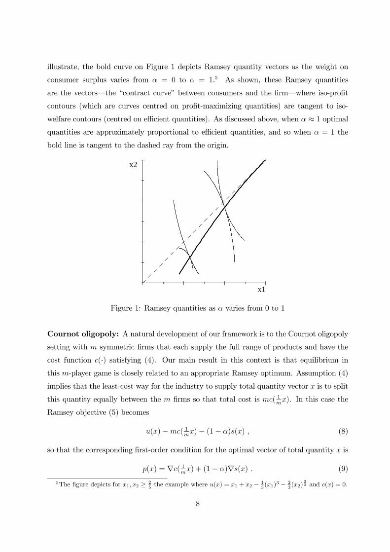
illustrate, the bold curve on Figure 1 depicts Ramsey quantity vectors as the weight on
consumer surplus varies from α = 0 to α = 1.5 As shown, these Ramsey quantities
are the vectors– the “contract curve”between consumers and the firm– where iso-profit
contours (which are curves centred on profit-maximizing quantities) are tangent to iso-
welfare contours (centred on effi cient quantities). As discussed above, when α ≈ 1 optimal
quantities are approximately proportional to effi cient quantities, and so when α = 1 the
bold line is tangent to the dashed ray from the origin.
x1
x2
Figure 1: Ramsey quantities as α varies from 0 to 1
Cournot oligopoly: A natural development of our framework is to the Cournot oligopoly
setting with m symmetric firms that each supply the full range of products and have the
cost function c(·) satisfying (4). Our main result in this context is that equilibrium in
this m-player game is closely related to an appropriate Ramsey optimum. Assumption (4)
implies that the least-cost way for the industry to supply total quantity vector x is to split
this quantity equally between the m firms so that total cost is mc( 1mx). In this case the
Ramsey objective (5) becomes
u(x)−mc( 1mx)− (1− α)s(x) , (8)
so that the corresponding first-order condition for the optimal vector of total quantity x is
p(x) = ∇c( 1mx) + (1− α)∇s(x) . (9)
5The figure depicts for x1, x2 ≥ 25 the example where u(x) = x1 + x2 − 1
3 (x1)3 − 2
3 (x2)32 and c(x) = 0.
8
Consider a candidate symmetric equilibrium in which each firm supplies quantity vector1mx (so that x is total supply). Then a firm must maximize its profit
π(y) = y · p(m−1mx+ y)− c(y)
by choosing y = 1mx, which from expression (2) has the first-order condition
p(x) = ∇c( 1mx) + 1
m∇s(x) . (10)
Comparing with (10) with (9) reveals that a symmetric Cournot equilibrium, if it exists, has
the same first-order conditions as the Ramsey problem (8) when the weight on consumers
is α = m−1m.
The following result establishes the existence and symmetry of Cournot equilibrium:
Proposition 1 Suppose there are m Cournot competitors, each of which supplies all n
products and has the same cost function c(x) satisfying (4). Then there exists a sym-
metric Cournot equilibrium in which quantities maximize the Ramsey objective (8) with
α = m−1m. There are no asymmetric equilibria. If in addition r(x) is concave there is only
one symmetric equilibrium.
Proof. We first rule out asymmetric equilibria. Consider a (possibly asymmetric) candi-
date equilibrium in which firm j supplies quantity vector xj, where x = Σjxj is the total
supply. At an asymmetric equilibrium, at least one firm must have xj 6= 1mx. In this
equilibrium firm j must maximize its profit
πj(y) = y · p(Σi 6=jxi + y)− c(y)
by choosing y = xj. In particular, it cannot be profitable to deviate from supplying
y = xj to supplying y = xj + ε(x−mxj), where ε is a scalar. Evaluating the derivative ofπj(x
j + ε(x−mxj)) with respect to ε at ε = 0 therefore yields
0 = [p(x)−∇c(xj) + xj ·Dp(x)] · (x−mxj)
= [p(x)−∇c(xj)− 1m
(x−mxj − x) ·Dp(x)] · (x−mxj)
≥ [p(x)−∇c(xj) + 1mx ·Dp(x)] · (x−mxj) , (11)
where the inequality (11) follows from the negative-definiteness of the matrix Dp(x). This
inequality is strict if xj 6= 1mx, which is the case for some firm in an asymmetric equilibrium,
9
and so summing (11) across the m firms we obtain
0 > −m∑j
( 1mx− xj) · ∇c(xj) ≥ m
∑j
[c(xj)− c( 1mx)] ≥ 0 , (12)
which is a contradiction. To see the second inequality in (12), note that the convexity of
c(·) implies c( 1mx)− c(xj) ≥ ( 1
mx− xj) · ∇c(xj), while the third inequality in (12) follows
directly from the convexity of c(·). We deduce that x cannot be equilibrium supply unless
it is symmetrically shared between firms.
Turning to equilibrium existence, note that the Ramsey objective (8) can be written
(1−α)r(x)+αu(x)−mc( 1mx). Suppose that quantity vector x solves this Ramsey problem
when α = m−1m. Since c is convex, it follows that choosing xj = 1
mx for each j maximizes
the function
(1− α)r(Σjxj) + αu(Σjx
j)− Σjc(xj) .
In particular, choosing y = 1mx maximizes the function
ρ(y) ≡ 1mr(m−1
mx+ y) + m−1
mu(m−1
mx+ y)− c(y) .
Now consider Cournot competition and a firm’s best response when its rivals each supply
quantity vector 1mx. This firm chooses its quantity vector y to maximize its profit
π(y) ≡ y · p(m−1mx+ y)− c(y)
= ρ(y)− m−1m
{u(m−1
mx+ y) + ( 1
mx− y) · p(m−1
mx+ y)
}≤ ρ(y)− m−1
mu(x) ,
where the inequality follows from the concavity of u. Since π( 1mx) = ρ( 1
mx)− m−1
mu(x), we
therefore have
π( 1mx)− π(y) ≥ ρ( 1
mx)− ρ(y) ≥ 0
where the final inequality follows since y = 1mx maximizes ρ(y). We deduce it is a Cournot
equilibrium for each firm to supply 1mx.
Finally, consider the uniqueness of equilibrium. We have already shown there are no
asymmetric equilibria, while expression (10) shows that any symmetric equilibrium satisfies
the first-order conditions for maximizing the Ramsey objective (8) with α = m−1m. This
Ramsey objective can be written as 1mr(x)+m−1
mu(x)−mc( 1
mx), and given that u is strictly
concave and c is convex, this is strictly concave if r(x) is concave. In this case, there is a
10
unique quantity vector x which satisfies the first-order condition (10), and hence a unique
symmetric equilibrium.
Thus, with symmetric convex cost functions there are no asymmetric Cournot equilibria,
and there exists a symmetric Cournot equilibrium in which total quantities maximize the
Ramsey objective (8) with α = m−1m. If revenue r is concave, there is a unique Cournot
equilibrium, which coincides with the (unique) optimum for the Ramsey objective (8)
with α = m−1m. In this sense, the Cournot problem and the (appropriately weighted)
Ramsey problem are the same. This generalizes the second remark in Bergstrom and
Varian (1985)– that a symmetric single-product Cournot oligopoly can be considered to
maximize a Ramsey objective– to the multiproduct context.
When c(x) is homogeneous degree 1, the number of suppliers has no impact on industry
costs and the Ramsey objectives (5) and (8) coincide. In this case, since consumer surplus
in the Ramsey problem (5) increases, and profit decreases, with α, we deduce that as the
number of competitors increases, a symmetric Cournot equilibrium delivers more surplus
to consumers and involves lower industry profit, and with many firms the equilibrium
quantities are approximately m−1mxw (where xw is the effi cient quantity vector). One can
also study how equilibrium prices depend on marginal costs by studying the simple Ramsey
problem, as we do below in section 3.3.
The analysis in Proposition 1 assumes firms are symmetric. Among other issues, this
assumption means one cannot study the impact of firm-specific cost shocks, for instance,
but only industry-wide cost shocks. When Cournot equilibria exist in asymmetric settings
it is straightforward to obtain first-order conditions for equilibrium prices. For example,
suppose that each firm has constant marginal costs, and firm j has the marginal cost vector
cj = (cj1, ..., cjn). Then if all firms supply all products in equilibrium, an argument similar
to (10) shows that equilibrium prices satisfy
p(x) = 1m
Σjcj + 1
m∇s(x) (13)
where 1m
Σjcj is the industry average vector of marginal costs.6 Thus, the Cournot equilib-
rium here corresponds to a the Ramsey optimum with weight on consumers α = m−1m
and
6This generalizes the first remark in Bergstrom and Varian (1985)– that equilibrium industry outputdepends only on the average marginal cost in the industry, not its distribution– to multiple products. Onecan show that this Cournot equilibrium exists if (i) inverse demands pi(x) are each weakly concave and(ii) that the cost vectors cj are “close enough”that each firm supplies all products in equilibrium.
11
a hypothetical monopolist with cost function c(x) = 1mx · [Σjc
j]. Another way to allow for
firm asymmetries is discussed in the following Bertrand model.
Bertrand oligopoly: Although it is not the focus of this paper, consider briefly one
way to model Bertrand competition in this framework. Bliss (1988) and Armstrong and
Vickers (2001, section 2) suggested a model where consumers buy all products from one
firm or another, so there is one-stop shopping, and firms therefore compete in terms of
the surplus they offer their customers. Each consumer has the same gross utility, u(x),
when they purchase quantity vector x from a firm, and this utility function is the same
at all firms. Firms compete by offering linear prices, so that a consumer obtains surplus
s(x) when they buy quantity x from a firm via linear prices, while firm i, say, obtains
profit r(x) − ci(x) from each customer where ci(x) is this firm’s constant-returns-to-scale
cost function. (Unlike the previous Cournot model, here it is straightforward to allow
firms to have different cost functions.) Consumers differ in their brand preferences for the
various firms, say due to the distances they must travel to reach them, and the number
of customers a firm attracts increases with the surplus s it offers and decreases with the
surplus its rivals offer.
In this framework, each firm’s strategy can be broken down into two steps: (i) choose
the most profitable way to deliver a given surplus to a customer, and (ii) choose how much
surplus to offer its customers. Step (i) is just the Ramsey problem as discussed above, and
a firm’s optimal prices take the form (6) where α now will reflect the firm’s competitive
constraints in step (ii) rather than concern for consumer welfare. In equilibrium there
is intra-firm effi ciency, but with cost differences across firms there will not in general be
industry-wide effi ciency (i.e., industry profits are not maximized subject to an overall
consumer surplus constraint).
The general analysis in this section has introduced the consumer surplus function s(x)
and shown its usefulness in analyzing the Ramsey monopoly problem and, by extension,
the symmetric Cournot oligopoly problem. In the rest of the paper we develop the analysis
of monopoly and oligopoly by supposing that s is homothetic in x. This specification
includes a number of familiar multiproduct demand systems, and has notably convenient
properties. In particular, the feature of equiproportionate quantity reduction that appeared
locally (for α ≈ 1 in the Ramsey problem or large m in the Cournot equilibrium) in the
analysis above, holds globally.
12
3 A family of demand systems
3.1 Homothetic consumer surplus
The family of demand systems on which we now focus is characterized by the property that
consumer surplus s(x) is a homothetic function of quantities x. We first describe which
demand systems have this property:
Proposition 2 Consumer surplus s(x) is homothetic in x if and only if utility u(x) can
be written in the form
u(x) = h(x) + g(q(x)) (14)
where h(·) and q(·) are homogeneous degree 1 functions and g(·) is concave with g(0) = 0.
Proof. First, note that we must have g(0) = 0 and g concave in q given that u(0) = 0
and u(·) is concave in x. (Since u is concave, when u takes the form (14) for given x the
function k → kh(x) + g(kq(x)) is too, so that g(·) is concave.)To show suffi ciency, note that (14) implies that inverse demand is
p(x) = ∇h(x) + g′(q(x))∇q(x) . (15)
Revenue is therefore
r(x) = x · p(x) = h(x) + g′(q(x))q(x) , (16)
where we used the fact that x·∇h(x) ≡ h(x) for a homogenous degree 1 function. Consumer
surplus s(x) is then
s(x) = g(q(x))− g′(q(x))q(x) , (17)
which is homothetic since s(x) is an increasing function of the homogenous function q(x).
(Since g is concave, g(q)− g′(q)q is an increasing function.)To show necessity, suppose that consumer surplus s(x) is homothetic, so that s(x) ≡
G(q(x)) for some increasing function G and some function q(x) which is homogeneous
degree 1. We can write G as G(q) ≡ g(q)− qg′(q) for another function g(·).7 Then
s(x̃/k) = g(q(x̃)/k)− q(x̃)
kg′(q(x̃)/k) =
d
dkkg(q(x̃)/k) . (18)
7Given any function G(·), one can generate the corresponding g(·) using the procedure
g(q) = −q∫ q
[G(q̃)/q̃2]dq̃ .
This function g(q) is concave given that G(q) is increasing.
13

Note that (1) can be generalized slightly so that s(x̃/k) = ddkku(x̃/k), and so (18) can be
integrated to yield
ku(x̃/k) = h(x̃) + kg(q(x̃)/k)
for some constant of integration h(x̃). Writing x = x̃/k this becomes
u(x) =h(kx)
k+ g(q(x)) .
Since this holds for all k we deduce that u(x) = h(x)+g(q(x)), where h(x) is homogeneous
degree 1.
This result implies that the set of demand systems in which consumer surplus is
homothetic in quantities is broader than that where consumer surplus is homothetic in
prices. Expressed as a function of prices, consumer surplus is the convex function v(p) =
maxx≥0{u(x) − p · x}. Duality implies that u(x) can be recovered from v(p) using the
procedure u(x) = minp≥0{v(p) + p · x}, and if v(p) is homothetic in p then u(x) =
minp≥0{v(p)+p ·x} is homothetic in x. Thus, the utility functions such that consumer sur-plus is homothetic in prices are simply the homothetic utility functions, i.e., where h ≡ 0
in (14), which is a subset of the family of preferences we study. In section 3.2 we discuss
familiar instances of the family (14) which do not have homothetic u(·).For the remainder of the paper we assume that utility u(x), as well as being increas-
ing and concave, can be written in the form (14). Some immediate observations on this
preference specification are:
• For a specific utility function u(x) it may not be obvious a priori whether it accords
with the form (14). However, Proposition 2 implies that this is the case whenever
consumer surplus, s(x) ≡ u(x) − x · ∇u(x), is homothetic, which in practice is easy
to check.
• Expression (15) implies that an equiproportionate change in quantities moves theprice vector along a straight line in the direction ∇q(x). In geometric terms, then,
quantity vectors on the ray joining x to the origin correspond to price vectors which
lie on the straight line starting at p(x) pointing in the direction ∇q(x).
• If u satisfies (14), then the modified environment in which a subset of these productsare removed also satisfies (14). That is, if a subset of products have quantities xi set
14
equal to zero, the utility function u defined on the remaining products continues to
satisfy (14).
• Since g is concave, the function g(q) − g′(q)q in (17) is an increasing function, so
surplus s increases with xi– and the Ramsey price for product i is above marginal
cost in (6)– if and only if q(·) increases with xi.
• When utility takes the form (14), the revenue function (16) takes a similar form, withthe same h and q (but with qg′(q) replacing g(q)). For this reason, a multiproduct
monopolist’s problem of maximizing profit– discussed below in section 3.3– is closely
connected to the consumer’s problem of maximizing surplus, where prices in the
consumer’s problem correspond to marginal costs in the firm’s problem.
• There are three degrees of freedom when choosing a demand system within the class–q(x), h(x) and g(q)– and expression (14) provides a useful toolkit for constructing
tractable multiproduct demand systems with particular desired properties. For this
purpose it is useful to know conditions for the resulting utility function u to be
concave. Suffi cient conditions to ensure that u in (14) is concave are that h and g
are concave and either: (i) q is concave and g is increasing; (ii) q is convex and g is
decreasing, or (iii) q is linear in x (which allows g to be non-monotonic).
For the remainder of this subsection we discuss in more detail the implications of this
utility specification for the corresponding demand system, denoted x(p). Given prices p,
the consumer with utility (14) can maximize her surplus with a simple two-step procedure.
We can write quantities x in the form
x ≡ q(x)× x
q(x). (19)
Here, x/q(x) is homogeneous degree zero and depends only on the ray from the origin on
which x lies, while q(x) is homogeneous degree 1 and measures how far along that ray x
lies, and so the decomposition (19) represents a generalized form of “polar coordinates”
for the quantity vector x. (The coordinate x/q(x) lies on the (n− 1)-dimensional surface
q ≡ 1.) Henceforth we refer to q(x) as “composite”quantity and x/q(x) as the “relative”
quantities.
We know already that (maximized) consumer surplus, s(x), depends on x only via
composite quantity q(x). More generally, consumer surplus with arbitrary quantities x
15

and prices p can be written in terms of the coordinates in (19) as
h(x) + g(q(x))− p · x = g(q(x))− q(x)p · x− h(x)
q(x). (20)
(Since the function p · x − h(x) is homogeneous degree 1, (p · x − h(x))/q(x) depends
only on the relative quantities x/q(x).) Since consumer surplus in (20) is decreasing in
(p · x− h(x))/q(x), the consumer should choose relative quantities to minimize this term,
regardless of her choice for composite quantity. Therefore, write
φ(p) ≡ minx≥0
:p · x− h(x)
q(x), (21)
which is an increasing and concave function of p. The envelope theorem implies that its
derivative is the optimal choice of relative quantities, so if we write x∗(p) ≡ ∇φ(p) the
consumer facing prices p chooses relative quantities x∗(p).8
Given the relative quantities, x∗(p), the optimal choice of composite quantity, say Q, is
easily derived. Consumer surplus in (20) with the optimal relative quantities is the concave
function g(Q)−Qφ(p). Write Q̂(φ) for the composite quantity which maximizes g(Q)−Qφ,which is necessarily weakly downward-sloping, so that Q̂(φ(p)) is the demand for composite
quantity given the price vector p. Price vectors with the same φ(p) induce the consumer
to choose the same composite quantity Q, and so φ(p) is the “composite” price which
corresponds to composite quantity q(x). Since the consumer chooses relative quantities
x∗(p) and composite quantity Q̂(φ(p)), from (19) the vector of quantities demanded at
prices p is
x(p) = Q̂(φ(p))× x∗(p) . (22)
Here, the function g(·) determines the shape the composite demand function Q̂(·), whilethe functions h(·) and q(·) combine to determine the form of composite price function φ(·).Expression (22) implies that cross or own-price demand effects are
∂xi∂pj
= Q̂(φ)φij + Q̂′(φ)φiφj . (23)
(Here, recall that x∗(p) = ∇φ(p), while subscripts to φ denote its partial derivatives.)
This is akin to the Slutsky Equation from classical demand theory. The first term in
(23) represents the substitution effect while staying on the same composite quantity (or
8There is a unique vector of relative quantities which solves (21) provided that h and q are quasi-concavewith one or both of them strictly so.
16
consumer surplus) contour, and the second term represents the impact of a price rise on
the composite quantity demanded. This second term is negative, while the first term is
negative if j = i and could be positive or negative when j 6= i. For instance, if utility is
homothetic then φ(p) is positive and homogenous degree 1, and expression (23) has the
sign ofφφijφiφj− −φQ̂
′(φ)
Q̂(φ). Here the first term is the elasticity of substitution of demand and
the second term is the elasticity of composite demand, and the relative sizes of these two
elasticities determines the sign of cross-price effects.
Since inverse demand p(x) in (15) induces demand x, it follows that
p = ∇h(x) + g′(Q)∇q(x)⇒ x(p) = Qx
q(x). (24)
In particular, for fixed Q any price vector of the form p = ∇h(x) + g′(Q)∇q(x) induces
the same composite demand Q, and hence the same consumer surplus s = g(Q)−Qg′(Q)
and composite price φ(p) = g′(Q). Conversely, since demand x(p) induces inverse demand
p, substituting (22) into the expression for inverse demand (15), and recalling that for
positive demand we have g′(Q̂(φ)) ≡ φ, reveals that
p ≡ ∇h(x∗(p)) + φ(p)∇q(x∗(p)) . (25)
(Alternatively, this expression is the first-order condition for problem (21).) Expression (25)
is the analogue for prices of the change of coordinates for quantities in (19), and decomposes
the price vector p into composite price, φ(p), and “relative prices”which in this context we
define to be x∗(p), i.e., the relative quantities which are optimal with prices p. From (24),
prices which induce relative quantities x∗ lie on the straight line φ : 7→ ∇h(x∗) + φ∇q(x∗),which is not necessarily a ray from the origin, while the coordinate φ(p) determines how
far along such a line the price vector lies.
3.2 Special cases
If u(·) is itself homothetic– for instance, if demand takes the familiar CES form– then(14) is trivially satisfied by setting h ≡ 0. In this case, expression (21) implies that φ(p)
is homogeneous degree 1, and x∗(p) = ∇φ(p) is homogeneous degree zero. More generally,
homothetic demand is an instance of the subclass of (14) where h takes the linear form
h(x) = a · x, when φ in (21) is a function that is homogenous degree 1 in the “adjusted”price vector (p− a).
17
Linear demand: Another instance of this subclass with linear h(·) is linear demand,where utility u(x) takes the quadratic form
u(x) = a · x− 12x ·M · x (26)
for constant vector a > 0 and (symmetric) positive-definite matrix M . Here, inverse
demands are p(x) = a − Mx, and utility takes the form (14) by writing h(x) = a · x,q(x) =
√x ·M · x and g(q) = −1
2q2. Here, ∇q(x) = Mx and so expression (24) implies
that the set of price vectors which correspond to the same relative quantities takes the
form p = a− tM · x for scalar t, which are rays originating from the vector of choke prices
a. It may be that q(x) and therefore s(x) decrease with xi when off-diagonal elements of
M are negative (which corresponds to products being complements).
Logit demand: Suppose that consumer demand takes the logit form
xi(p) =eai−pi
1 +∑
j eaj−pj
, (27)
where a = (a1, ..., an) is a constant vector. It follows that inverse demand is
pi(x) = ai − logxi
1− q(x), (28)
where q(x) ≡∑
j xj is total quantity. This inverse demand function (28) integrates to give
the utility function
u(x) = a · x−∑j
xj log xj − (1− q(x)) log (1− q(x)) .
(As with any demand system resulting from discrete choice, the utility function is only
defined on the domain Σixi ≤ 1.9) This utility can be written in the required form (14) as
u(x) = a · x+∑i
xi logq(x)
xi︸ ︷︷ ︸h(x)
+ g(q(x)) . (29)
Here, h(x) as labelled is homogenous degree 1, as is total output q(x), while g(q) is equal
to the entropy function g(q) = −q log q− (1− q) log(1− q), which is concave in 0 ≤ q ≤ 1.
Since g′(q) = log(1− q)− log q, demand for composite quantity as a function of composite
9If one wishes only to consider non-negative prices, from (28) one should further restrict attention toquantity vectors which satisfy xi ≤ (1− Σjxj)e
ai for i = 1, ..., n.
18
price takes the logistic form.10 With logit, as with homogeneous goods, consumer surplus
is a function only of total quantity, and product differentiation is reflected separately in the
h(x) term. Since ∇q(x) ≡ (1, ..., 1), the set of prices which correspond to the same relative
quantities takes the form p + (t, ..., t), as can be seen directly from (27). This contrasts
with the subclass with linear h(x), where these lines were not parallel but emanated from
a point. More generally, with any demand system in the subclass with linear q(x) = b · x,the set of prices which correspond to quantity vectors on a given ray from the origin take
the form of parallel straight lines.
Systems of strictly complementary products: A common situation is where con-
sumers purchase a single unit of a “base product”, and then combine this with variable
quantities of one or more complementary products. For instance, a consumer may need
to gain entry to a theme park before they can go on the rides (Oi, 1971), or needs to buy
a printer along with a suitable quantity of ink in order to print. To illustrate how these
situations sometimes fit into our framework, suppose there is a continuum of consumers
indexed by scalar θ, where the type-θ consumer has gross utility U(y) + θ if she consumes
quantity y of the combined service. (The following discussion also applies if y is a vector of
multiple services.) Adding over the population of consumers implies that aggregate gross
utility if x1 consumers (those with the highest value of θ) each consume quantity y of
combined service takes the form x1U(y) + g(x1) for some increasing concave function g(·),where g is determined by the distribution of θ. If x2 denotes the quantity of combined
service across all consumers, so that x2 = x1y, it follows that aggregate utility in terms of
the quantity vector (x1, x2) is
u(x1, x2) = x1U(x2/x1) + g(x1) . (30)
Clearly, this utility function fits into our family (14), where h(x) = x1U(x2/x1) and com-
posite quantity is just q(x) = x1. This is another instance of the subclass with linear
q(x), but here s(x) is a function only of x1, the number of active consumers. The set of
prices which correspond to the same relative quantities– i.e., the same usage per active
consumer– are horizontal lines with p2 constant.
10Anderson et al. (1988) have previously noted the connection between logit demand and entropy. Theentropy function makes it diffi cult to obtain closed-form solutions for optimal prices or quantities withlogit demand. However, if we modify (29) slightly so that g(q) ∝ q(1− q), demand for composite quantityis linear rather than logistic and explicit formulas can be obtained.
19

3.3 Analysis
In this section we discuss how to maximize welfare and profit, as well as calculate oligopoly
outcomes, when the demand system satisfies (14) and the cost function satisfies
c(x) is convex and homogeneous degree 1. (31)
Consider again the problem of maximizing a weighted sum of profit and consumer surplus.
If 0 ≤ α ≤ 1 is the relative weight on consumer surplus, the Ramsey objective (5) is
[r(x)− c(x)] + αs(x) = αg(q(x)) + (1− α)g′(q(x))q(x)− q(x)c(x)− h(x)
q(x). (32)
Here, we used the formulas (16)-(17).
As with the consumer’s problem in section 3.1, the Ramsey problem can conveniently
be solved by means of the change of variables (19). Expression (32) shows how the Ramsey
objective can be written in terms of composite quantity q(x) and the relative quantities
x/q(x). Expression (32) is decreasing in the term (c(x) − h(x))/q(x), and so relative
quantities should be chosen to minimize this term. As in (21), write
κ = minx≥0
:c(x)− h(x)
q(x), (33)
which is solved by choosing relative quantities x = x∗, say. (Since the quantity vector
which minimizes (33) is indeterminate up to a scaling factor, as in section 3.1 we normalize
x∗ so that q(x∗) = 1.11) We deduce that maximizing any Ramsey objective involves
choosing the same relative quantities x∗, in contrast to the case depicted in Figure 1. In
particular, profit-maximizing quantities (α = 0) are proportional to the effi cient quantities
corresponding to marginal-cost pricing (α = 1). That is, the unregulated firm has an
incentive to choose its relative quantities in an effi cient manner, and the sole ineffi ciency
arises from it supplying too little composite quantity.
Given this choice for relative quantities, the optimal choice for composite quantity Q
is easily derived. Expression (32) with relative quantities x∗ is the function
αg(Q) + (1− α)g′(Q)Q− κQ . (34)
11There is a unique vector of relative quantities which solves (33) provided that (c−h) is quasi-convex andq is quasi-concave with one of them strictly so. To illustrate this analysis, suppose that q(x1, x2) =
√x1x2,
h(x1, x2) = 0 and c(x1, x2) =√c21x
21 + c22x
22. Then one can check that x
∗ = ( c2c1 ,c1c2
) and κ =√
2c1c2.
20

(A suffi cient condition for (34) to be concave in Q for all α is that “composite revenue”
g′(Q)Q be concave.) The vector of quantities which solves the Ramsey problem is then
Qx∗, where Q maximizes expression (34). The optimal composite quantity Q increases
with α and decreases with κ, and satisfies the Lerner formula
g′(Q)− κg′(Q)
= (1− α)η(Q) , (35)
where
η(Q) ≡ −Qg′′(Q)
g′(Q)(36)
is the elasticity of inverse demand for composite quantity.
Since relative quantities are the same in all Ramsey problems, so too are relative price-
cost margins. As discussed in section 3.1, this is because an equiproportionate reduction in
effi cient quantities causes the price vector to move in a straight line away from the vector
of marginal costs. In more detail, the optimal quantities for the Ramsey problem are Qx∗,
where Q satisfies (35), and in particular let the composite quantity which maximizes total
surplus (i.e., when α = 1) be denoted Qw, so that g′(Qw) = κ. Then the price-cost margins
in the Ramsey problem with composite quantity Q are
p(Qx∗)−∇c(Qx∗) = p(Qx∗)−∇c(Qwx∗)
= p(Qwx∗)−∇c(Qwx∗) + [g′(Q)− g′(Qw)]∇q(x∗)
= [g′(Q)− κ]∇q(x∗) . (37)
(Here, the first equality follows from∇c being homogeneous degree zero, the second followsfrom (15), and the final equality follows since prices equal marginal costs and g′ = κ when
Q = Qw.) These margins are proportional to ∇q(x∗), and shrink equiproportionately whenQ is larger. Product i is used as a loss leader, in the sense that its price is below marginal
cost, in each Ramsey problem when composite quantity q decreases with xi at x∗.
By virtue of the Ramsey-Cournot result in Proposition 1, these properties extend to
symmetric Cournot oligopoly. To summarise:
Proposition 3 Suppose that utility takes the form (14) and cost takes the form (31). As
more weight is placed on consumer surplus in the Ramsey problem, the composite quan-
tity increases, the composite price decreases, each individual quantity increases equipropor-
tionately, and each price-cost margin contracts equiproportionately. The same is true in
symmetric Cournot equilibrium as the number of firms increases.
21
An important special case involves constant marginal costs, so that c(x) ≡ c · x fora constant vector of marginal costs c = (c1, ..., cn). In this case, κ in (33) is simply φ(c)
where the function φ(·) is defined in (21), while x∗ = x∗(c). In this context, consider
how optimal prices relate to the firm’s costs. This analysis is most transparent using the
change of variables for prices (and costs) in (25), so that φ(p) is the composite price and
x∗(p) are relative prices (and similarly for the cost vector). As discussed earlier, in any
Ramsey problem it is optimal to choose relative quantities equal to the relative quantities
which correspond to effi cient marginal-cost pricing. This immediately implies that it is
optimal to choose relative prices equal to the firm’s relative costs, so that x∗(p) = x∗(c).
The optimal markup of composite price over composite cost is then given by (35), and
the optimal composite price, φ(p), decreases with the weight on consumer surplus, α, and
increases with composite cost, φ(c).12
What does this mean for price-cost relationships: how does pi depend on cj? Expres-
sions (35) and (37) imply that optimal prices satisfy
p− c = (1− α)η(Q)g′(Q)×∇q(x∗(c)) . (38)
Consider first the subclass where h takes the linear form h(x) = a · x. Since optimalquantities are Qx∗(c), expression (15) shows that prices satisfy
p− a = g′(Q)×∇q(x∗(c)) . (39)
Putting (38) and (39) together implies that
p− c =(1− α)η(Q)
1− (1− α)η(Q)× (c− a) . (40)
In particular, when preferences are homothetic, so that a = 0, we obtain the familiar result
that proportional price-cost markups are the same across products.
In the iso-elastic case where η is constant, expression (40) implies that the optimal
price for product i depends only on ci, not on any other product’s cost, and so there is
no “cross-cost” passthrough in prices, even though there may be substantial cross-price
effects in the demand system. Moreover, provided that the consumer can obtain positive
12Since the profit-maximizing firm’s choice of composite quantity falls with φ(c), and since consumersurplus, s, is an increasing function of composite quantity, we deduce that the firm necessarily offers alower level of consumer surplus when unit cost ci increases. Our family of demand systems thereforeexcludes the possibility explored by Edgeworth (1925) that imposing a linear tax on a product suppliedby a multiproduct monopolist could reduce all of its prices.
22
utility with a subset of products (e.g., if ρ > 0 in the CES specification), the optimal price
for one product is unaffected if the firm is restricted to offer a subset of products (or even
just that product).13 For instance, if u is homothetic and g(Q) = 1γQγ, where 0 < γ < 1,
then η ≡ 1− γ and (40) implies that the most profitable prices (i.e.,when α = 0) are
p =1
γc .
Likewise, with linear demand we have η ≡ −1 and expression (40) implies that the profit-
maximizing prices are14
p = 12(a+ c) . (41)
More generally within this subclass with linear h, expression (40) and the fact that the
most profitable Q decreases with each cost implies that all cross-cost passthrough terms
for pi have the same sign as (ai − ci)η′(Q).15
Alternatively, consider the subclass where composite quantity takes the linear form
q(x) = b · x. Then (38) implies that
p− c = (1− α)η(Q)g′(Q)× b . (42)
In the example with complementary products where utility is (30) and b = (1, 0), this
expression implies there is marginal-cost pricing for usage (p2 = c2), and in particular
changes in c1 have no impact on p2. However, there is cross-cost passthrough in the other
direction: since the optimal Q decreases with both costs, it follows that p1 increases or
decreases with c2 according to whether η(Q)g′(Q) decreases or increases with Q. In the
logit example utility is (29) and b = (1, ..., 1), so the price-cost margin pi−ci is the same for13Shugan and Desiraju (2001) discuss these points in the context of linear demand with two products.
In the context of product line pricing, Johnson and Myatt (2015) explore when it is that a firm’s optimalprice for one product variant can be calculated by supposing that the firm only supplies that variant.(They consider both monopoly and Cournot settings.)14It usually makes sense only to consider non-negative quantities, in which case (41) is only valid if a
and c are such that the optimal quantities, x = 12M
−1 · (a − c), are positive. In the case of substitutes,where the matrix M necessarily has all non-negative elements, a necessary condition for this is that eachai ≥ ci. (When M has all non-negative elements, the operation x 7→ Mx takes Rn+ into itself.) However,with complements, it is possible to have all xi positive and some ai − ci negative. In such cases, (41)indicates that pi < ci for those products with ai < ci.15One can analyze how the optimal quantity supplied of one product is affected by cost changes to
other products in a similar manner to the consumer demand expression (23). For instance, since profit-maximizing quantities satisfy the first-order condition∇r(x) = c, where c is the vector of constant marginalcosts, there will be a dependence of one product’s supply on another product’s cost unless r(x) is additivelyseparable in quantities, which is (essentially) only the case if demand for one product does not depend onother prices.
23
each product i, and the common markup (1−α)η(Q)g′(Q) = (1−α)/(1−Q), increases with
Q < 1. Since the optimal Q decreases with each ci, it follows that cross-cost passthrough
is negative and one product’s price decreases with each other product’s cost.
As shown in Proposition 1, with m firms each with a cost function satisfying (31) the
outcome with Cournot oligopoly coincides with the Ramsey optimum, provided we set the
weight on consumer interests in the Ramsey problem equal to α = m−1m. With our demand
system (14), then, expression (35) implies that equilibrium composite quantity satisfies
g′(Q)− κg′(Q)
=1
mη(Q) ,
and Proposition 3 has the corollary that as the number of competitors increases composite
quantity increases, composite price decreases, each individual quantity increases equipro-
portionately, and each price-cost margin contracts equiproportionately. In addition, when
c(x) = c · x and h(x) = a · x, expression (40) implies that
p− c =η(Q)
m− η(Q)× (c− a) . (43)
As in the Ramsey problem, cross-cost passthrough terms for product i have the same sign
as (ai − ci)η′(Q). (Here, a change in one product’s cost is assumed to be industry-wide,
not firm-specific.) So if η(Q) is constant, then the equilibrium price for one product does
not depend on the costs of other products, and nor is one product’s price affected when
only a subset of products is supplied by the industry.
Firm-specific cost shocks can be analyzed using expression (13). Thus, provided each
firm supplies all products in equilibrium, when h(x) = a · x expression (43) continues toapply provided that the vector c is interpreted to be the industry average vector of marginal
costs. To illustrate, with linear demand the equilibrium price for product i with m firms is
pi = 1m+1
(ai + Σjc
ji
),
where cji is firm j’s cost for product i. Thus an increase in cost cji will be passed through
at rate 1m+1
to product i’s price and will have no impact on prices for other products.
3.4 Regulation with asymmetric information about costs
When the demand system falls within the family (14), we have seen that the unregulated
monopolist will choose an effi cient pattern of relative quantities, even though it supplies too
24

little composite quantity. This suggests that, in some circumstances at least, the optimal
way to regulate market power when the firm has private information about its costs is to
control only its composite quantity, leaving it free to choose relative quantities to reflect
its private information.
To explore this issue, we consider optimal regulation of multiproduct monopoly by ex-
tending the analysis of the single-product case by Baron and Myerson (1982). Specifically,
there is common knowledge about the demand system, which we assume satisfies (14), but
the firm has private information about its costs. In particular, suppose the firm has the
vector of constant marginal costs, c = (c1, ..., cn). Optimal regulation can be analyzed by
way of a “direct”scheme whereby the firm reports its cost vector, say c̃, to the regulator,
and conditional on this report the firm is instructed to supply a vector of quantities X and
receives a net transfer T funded by consumers (in addition to the usual revenue r(X)).
The revelation principle implies that we can restrict attention to mechanisms in which the
firm is given an incentive to report its cost vector truthfully, so that c̃ = c. The regulator
places weight 0 ≤ β ≤ 1 on profit relative to consumer surplus, where profit includes the
transfer T and consumer surplus includes the deduction for the transfer T .
Expression (25) implies we can decompose the cost vector c into composite costs, φ(c),
and relative costs, x∗(c), so that c = ∇h(x∗(c))+φ(c)∇q(x∗(c)). From this perspective, thefirm reports its private cost information in terms of coordinates (φ̃, x̃∗), and conditional on
this report the regulator instructs it to supply composite quantity Q and relative quantities
x∗.
It is useful to study first the situation where the coordinate x∗(c) can be directly
observed by the regulator, before considering the more realistic situation where it is not.16
If the regulator knows the firm’s costs satisfy x∗(c) = x∗, say, then (25) implies that the
cost vector lies on the straight line∇h(x∗)+κ∇q(x∗), where κ denotes the firm’s compositecost, φ(c). However, the regulator does not know where on this line the cost vector lies,
and so needs to solve a one-dimensional screening problem. The following result describes
optimal regulation in this situation, which adapts by-now standard arguments in Baron
16This approach is similar to that in Armstrong (1996, section 4.4) and Armstrong and Vickers (2001,Proposition 5), where a multidimensional screening problem is solved by supposing that the principalcan observe all-but-one dimension of the agent’s private information, and then finding conditions whichensure that the incentive scheme offered to these group of agents does not actually depend on the observedparameters.
25
and Myerson (1982, section 3) to our multiproduct context.17 (The proof of this result is
in the appendix to this paper.)
Lemma 1 Suppose the regulator knows the firm’s cost vector satisfies x∗(c) = x∗ and
believes the firm’s composite cost κ = φ(c) has cumulative distribution function F (κ | x∗)and associated density function f(κ | x∗). Provided (44) weakly increases with κ, optimalregulation requires the firm with composite cost κ to supply the composite quantity, Q̂(φ(p)),
corresponding to the composite price
φ(p) = κ+ (1− β)F (κ | x∗)f(κ | x∗) (44)
and to supply the effi cient relative quantities x∗.
This result shows that relative quantities are not distorted from the effi cient relative
quantities, x∗, while if β < 1 expression (44) shows that composite price is above composite
cost, and hence that composite quantity is below the effi cient level, in order to reduce the
rent enjoyed by the firm. Although the result is expressed as the firm being required to
offer effi cient relative quantities, it is clear that the firm would anyway choose to do this if
it had discretion to choose relative quantities.
Consider now the more natural case where the regulator cannot observe x∗(c). In
general, with current techniques this seems to be an intractable problem. However, in
the special case where the distribution for c is such that φ(c) and x∗(c) are independent
random variables, the previous result provides the solution:
Proposition 4 Suppose the distribution for c is such that φ(c) and x∗(c) are stochastically
independent, where the firm’s composite cost κ = φ(c) has cumulative distribution function
F (κ) and associated density function f(κ). Provided (45) weakly increases with κ, optimal
regulation requires the firm with composite cost κ to supply the composite quantity, Q̂(φ(p)),
corresponding to the composite price
φ(p) = κ+ (1− β)F (κ)
f(κ)(45)
and to supply the effi cient relative quantities x∗(c).
17Baron and Myerson also show how to solve the problem when (44) is not increasing. Sappington(1983) solves a distinct multiproduct regulation problem with scalar private information, where the firmcan affect the balance between fixed and variable costs.
26

Proof. If the two cost coordinates are independent, the regulation of composite quantity
in Lemma 1 does not depend on x∗(c). (Not only is the required composite quantity
independent of x∗(c) in (44), but so is the associated transfer function T (κ) in expression
(53) in the appendix.) Consider therefore the regulatory scheme in which, if the firm
reports its composite cost is κ and its relative costs are x̃∗, it is instructed to supply the
composite quantity corresponding to the composite price (45), it is instructed to supply
relative quantities x̃∗, and it receives the transfer T (κ) in (53). For any given report κ,
then, the firm will choose its report x̃∗ to maximize its profit. As in section 3.3 this is
always achieved by minimizing (33), so that the firm reports its true relative costs x∗(c).
By construction, this policy therefore implements the optimal policy when the regulator
could observe x∗(c) directly, and so the policy must also be optimal when the regulator
cannot observe x∗(c) directly.
This optimal scheme gives an incentive for the firm to supply higher composite quantity,
but does not attempt to influence its choice of relative quantities.18 Intuitively, when φ(c)
and x∗(c) are stochastically independent the firm is always happy for the regulator to
observe its relative cost parameter x∗(c) but not its composite cost φ(c). That is, for a
given composite quantity, the firm and the regulator have aligned preferences with respect
to the choice of relative quantities. The regulator gains by delegating to the firm the
choice of relative quantities, to enable the firm to make use of its private information
about relative costs, and it does this by using a transfer scheme which depends only on
the composite quantity supplied. However, if φ(c) and x∗(c) are correlated, observing the
firm’s relative costs x∗(c) is informative about the firm’s composite cost φ(c), which gives
the firm an incentive to mis-report its relative costs as well as its composite cost.
To illustrate Proposition 4, suppose that there are two products and utility takes the
additive form u(x) =√x1 +
√x2, which can be written as (14) with h = 0, q(x) =(√
x1 +√x2)2and g(Q) =
√Q. In this case (33) implies
κ = φ(c) =1
1c1
+ 1c2
, (46)
while x∗(c) = (( c2c1+c2
)2, ( c1c1+c2
)2) depends only on the cost ratio c1c2. Thus the method
requires that the distribution for (c1, c2) be such that 1c1
+ 1c2and c1
c2are independent
18Note that when β = 1, so that the regulator cares only about unweighted surplus, expression (44)implies that Q does not depend on x∗ regardless of the distribution for c. In this case, it is optimal to setprices equal to marginal costs for all firms, as discussed in Loeb and Magat (1979).
27

variables. Since the sum and ratio of two i.i.d. exponential variables are independent,
the method works if each ci is an independent draw from a distribution such that 1/c is
exponentially distributed.19 Specifically, suppose that each ci has support [0,∞) and CDF
Pr {c ≤ t} = e−1t . Then 1/κ is the sum of two exponential variables and so κ has CDF
F (κ) = (1 + 1κ)e−
1κ and corresponding density f(κ) = 1
κ3e−
1κ . Expression (45) then implies
that optimal composite price for the type-κ firm is κ + (1 − β)κ2(1 + κ), which increases
with κ as required, and (52) then implies that the optimal individual prices are
pi = ci [1 + (1− β)κ(1 + κ)] (47)
where κ is the function of c given by (46).20
In expression (47) there is marginal-cost pricing for those firms with κ = 0, and so
pi = ci whenever the other product has minimum cost cj = 0. The regulated price for one
product is an increasing function of the other product’s cost, even though this demand
system has no cross-price effects and there is no statistical correlation in costs across
products. Note also that all types of firm participate in the mechanism, and unlike in
Armstrong (1996, section 3) there is no “exclusion” in the optimal scheme. However, so
long as β < 1, when the firm has high costs the prices in (47) are above the unregulated
profit-maximizing prices (which with this demand system are pi = 2ci), a possibility that
was noted in the single-product context by Baron and Myerson (1982, page 292).
Similar analysis could be applied in the alternative situation with price-cap regulation,
when transfer payments to the firm are not feasible and instead the regulator specifies the
set of quantity (or price) vectors from which the firm is permitted to choose. If, hypotheti-
cally, the regulator could observe the firm’s relative costs x∗(c), but not its composite cost
φ(c), it could calculate the optimal set of quantity vectors from which the firm can select,
which plausibly will all be proportional to the effi cient pattern x∗(c).21 In this case, the
regulator can let the iso-x∗ firms choose from a set of composite quantities, and let the
firm choose its pattern of relative quantities freely. When φ(c) and x∗(c) are stochastically
19Another way to describe this distribution is that ci comes from an inverse-χ2 distribution with 2degrees of freedom.20Another example which works nicely is when h = 0 and q(x) =
√x1x2, so that φ(c) = 2
√c1c2. In
this case Proposition 4 applies when the distribution for (c1, c2) is such that the product c1c2 and theratio c1/c2 are stochastically independent, which is the case when each ci is an independent draw from alog-normal distribution.21It is possible that it is optimal to leave gaps in the set of permitted quantities. Even in the sim-
pler single-product case, Alonso and Matouschek (2008) and Amador and Bagwell (2014) show how theregulator sometimes chooses to leave gaps in the set of permitted prices.
28

independent, it follows that the permitted set of composite quantities does not depend on
x∗(c), and this set of composite quantities then constitutes the optimal price-cap scheme.
4 Conclusions
In this paper we have studied a range of multiproduct pricing questions in terms of con-
sumer surplus considered as a function of quantities. With a monopolist, this is the classical
profit-maximization problem, or more generally the Ramsey problem of welfare maximiza-
tion subject to a profit constraint. With oligopoly, by contrast, the multiproduct pricing
question is one of equilibrium among independent firms, not optimization by a single
decision-maker. We have shown, however, that in perhaps the most natural multiprod-
uct oligopoly model, with symmetric Cournot firms, there is Ramsey-Cournot equivalence.
With suitable welfare weights as between profit and consumer surplus, Ramsey quanti-
ties are Cournot equilibrium quantities, and vice versa. Solutions to Ramsey optimization
problems are therefore equilibrium solutions too.
The other main aim of the paper has been to show how multiproduct monopoly analysis
is made simpler when consumer surplus is a homothetic function of quantities. Whether
the firm’s objective is profit or a Ramsey combination of profit and consumer surplus, it
optimizes by selecting effi cient (i.e., welfare-maximizing) quantities scaled back equipropor-
tionately. The resulting optimal markups yield, for example, transparent results on mul-
tiproduct cost passthrough, including instances of without cross-cost passthrough. With
Ramsey-Cournot equivalence, these results extend to the Cournot oligopoly setting with
symmetric firms.
The family of demand systems with consumer surplus a homothetic function of quan-
tities is of course restrictive. But it includes a number of familiar yet diverse special cases,
including CES and linear demands and discrete choice models such as logit. Moreover,
it shows how those special cases are themselves instances of wider sub-classes of demand
systems, involving h(x) ≡ 0, linear h(x) and linear q(x) respectively.
Finally, the family of demand systems analyzed in this paper provides a natural basis
on which to explore the intuition that regulation of multiproduct monopoly should focus
on the general level of prices and not the pattern of relative prices. Indeed we showed how
that intuition can sometimes be precisely correct, thereby contributing to the theory of
multi-dimensional screening.
29
Appendix
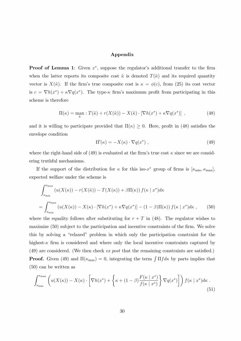
Proof of Lemma 1: Given x∗, suppose the regulator’s additional transfer to the firm
when the latter reports its composite cost κ̃ is denoted T (κ̃) and its required quantity
vector is X(κ̃). If the firm’s true composite cost is κ = φ(c), from (25) its cost vector
is c = ∇h(x∗) + κ∇q(x∗). The type-κ firm’s maximum profit from participating in this
scheme is therefore
Π(κ) = maxκ̃
: T (κ̃) + r(X(κ̃))−X(κ̃) · [∇h(x∗) + κ∇q(x∗)] , (48)
and it is willing to participate provided that Π(κ) ≥ 0. Here, profit in (48) satisfies the
envelope condition
Π′(κ) = −X(κ) · ∇q(x∗) , (49)
where the right-hand side of (49) is evaluated at the firm’s true cost κ since we are consid-
ering truthful mechanisms.
If the support of the distribution for κ for this iso-x∗ group of firms is [κmin, κmax],
expected welfare under the scheme is∫ κmax
κmin
(u(X(κ))− r(X(κ̃))− T (X(κ)) + βΠ(κ)) f(κ | x∗)dκ
=
∫ κmax
κmin
(u(X(κ))−X(κ) · [∇h(x∗) + κ∇q(x∗)]− (1− β)Π(κ)) f(κ | x∗)dκ , (50)
where the equality follows after substituting for r + T in (48). The regulator wishes to
maximize (50) subject to the participation and incentive constraints of the firm. We solve
this by solving a “relaxed” problem in which only the participation constraint for the
highest-κ firm is considered and where only the local incentive constraints captured by
(49) are considered. (We then check ex post that the remaining constraints are satisfied.)
Proof. Given (49) and Π(κmax) = 0, integrating the term∫
Πfdκ by parts implies that
(50) can be written as∫ κmax
κmin
(u(X(κ))−X(κ) ·
[∇h(x∗) +
{κ+ (1− β)
F (κ | x∗)f(κ | x∗)
}∇q(x∗)
])f(κ | x∗)dκ .
(51)
30
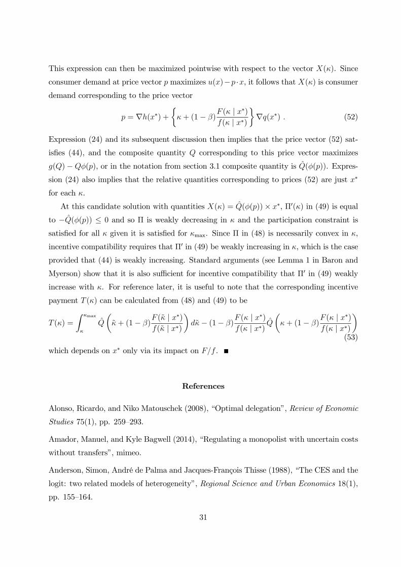
This expression can then be maximized pointwise with respect to the vector X(κ). Since
consumer demand at price vector p maximizes u(x)−p ·x, it follows that X(κ) is consumer
demand corresponding to the price vector
p = ∇h(x∗) +
{κ+ (1− β)
F (κ | x∗)f(κ | x∗)
}∇q(x∗) . (52)
Expression (24) and its subsequent discussion then implies that the price vector (52) sat-
isfies (44), and the composite quantity Q corresponding to this price vector maximizes
g(Q)−Qφ(p), or in the notation from section 3.1 composite quantity is Q̂(φ(p)). Expres-
sion (24) also implies that the relative quantities corresponding to prices (52) are just x∗
for each κ.
At this candidate solution with quantities X(κ) = Q̂(φ(p))× x∗, Π′(κ) in (49) is equal
to −Q̂(φ(p)) ≤ 0 and so Π is weakly decreasing in κ and the participation constraint is
satisfied for all κ given it is satisfied for κmax. Since Π in (48) is necessarily convex in κ,
incentive compatibility requires that Π′ in (49) be weakly increasing in κ, which is the case
provided that (44) is weakly increasing. Standard arguments (see Lemma 1 in Baron and
Myerson) show that it is also suffi cient for incentive compatibility that Π′ in (49) weakly
increase with κ. For reference later, it is useful to note that the corresponding incentive
payment T (κ) can be calculated from (48) and (49) to be
T (κ) =
∫ κmax
κ
Q̂
(κ̃+ (1− β)
F (κ̃ | x∗)f(κ̃ | x∗)
)dκ̃− (1− β)
F (κ | x∗)f(κ | x∗) Q̂
(κ+ (1− β)
F (κ | x∗)f(κ | x∗)
)(53)
which depends on x∗ only via its impact on F/f .
References
Alonso, Ricardo, and Niko Matouschek (2008), “Optimal delegation”, Review of Economic
Studies 75(1), pp. 259—293.
Amador, Manuel, and Kyle Bagwell (2014), “Regulating a monopolist with uncertain costs
without transfers”, mimeo.
Anderson, Simon, André de Palma and Jacques-François Thisse (1988), “The CES and the
logit: two related models of heterogeneity”, Regional Science and Urban Economics 18(1),
pp. 155—164.
31

Armstrong, Mark (1996), “Multiproduct nonlinear pricing”, Econometrica 64(1), pp. 51—
75.
Armstrong, Mark, and John Vickers (2001), “Competitive price discrimination”, Rand
Journal of Economics 32(4), pp. 579-605.
Baron, David, and Roger Myerson (1982), “Regulating a monopolist with unknown costs”,
Econometrica 50(4), pp. 911—930.
Baumol, William, and David Bradford (1970), “Optimal departures from marginal cost
pricing”, American Economic Review 60(3), pp. 265—283.
Bergstrom, Theodore, and Hal Varian (1985), “Two remarks on Cournot equilibria”, Eco-
nomics Letters 19(1), pp. 5—8.
Besanko, David, Jean-Pierre Dubé and Sachin Gupta (2005), “Own-brand and cross-brand
retail pass-through”, Marketing Science 24(1), pp. 123-137.
Bliss, Christopher (1988), “A theory of retail pricing”, Journal of Industrial Economics
36(4), pp. 375—391.
Bulow, Jeremy, and Paul Klemperer (2012), “Regulated prices, rent seeking, and consumer
surplus”, Journal of Political Economy 120(1), pp. 160—186.
Edgeworth, Francis (1925), Papers Relating to Political Economy, McMillan and Co.
Gorman, W.M. (1961), “On a class of preference fields”, Metroeconomica 13(2), pp. 53-56.
Johnson, Justin, and David Myatt (2015), “The properties of product line prices”, Inter-
national Journal of Industrial Organization 143, pp. 182—188.
Laffont, Jean-Jacques, and Jean Tirole (1993), A Theory of Incentives in Procurement and
Regulation, MIT Press.
Loeb, Martin, and Wesley Magat (1979), “A decentralized method for utility regulation”,
Journal of Law and Economics 22(2), pp. 399—404.
Monderer, Dov, and Lloyd Shapley (1996), “Potential games”, Games and Economic Be-
havior 14(1), pp. 124—143.
Moorthy, Sridhar (2005), “A general theory of pass-through in channels with category
management and retail competition”, Marketing Science 24(1), pp. 110-122.
32
Oi, Walter (1971), “ADisneyland dilemma: two-part tariffs for a MickeyMouse monopoly”,
Quarterly Journal of Economics 85(1), pp. 77—96.
Sappington, David (1983), “Optimal regulation of a multiproduct monopoly with unknown
technological capabilities”, Bell Journal of Economics 14(2), pp. 453—463.
Shugan, Steven, and Ramarao Desiraju (2001), “Retail product-line pricing strategy when
costs and products change”, Journal of Retailing 77(1), pp. 17—38.
Slade, Margaret (1994), “What does an oligopoly maximize?”, Journal of Industrial Eco-
nomics 42(1), pp. 45-61.
Vives, Xavier (1999), Oligopoly Pricing, MIT Press.
Weyl, Glen, and Michal Fabinger (2013), “Pass-through as an economic tool: principles of
incidence under imperfect competition”, Journal of Political Economy 121(3), pp. 528-583.
33