Multiprocessor Platforms for Natural LanguageProcessing

Henrique Ribeiro Vasconcelos Costa

Dissertacao para obtencao do Grau de Mestre em

Engenharia Informatica e de Computadores

Juri

Presidente: Doutor Jose DelgadoOrientador: Professor David Martins de MatosArguente: Professor Nuno Roma

Maio de 2009

Agradecimentos

Em primeiro lugar gostaria de agradecer ao Prof. David Matos pela sua orientacao, colaboracao e

paciencia, sem as quais esta tese nunca teria terminado.

Os meus agradecimentos vao tambem para a IBM Corporation, que atraves do Virtual Loaner Pro-

gram disponibilizou processadores Cell Broadband Engine.

Contribuiram tambem para este trabalho de pesquisa o Georgia Institute of Technology, o seu Sony-

Toshiba-IBM Center of Competence e a National Science Foundation, disponibilizando acesso aos seus

servidores.

Quero tambem agradecer aos meus colegas e amigos, pelo apoio e companhia nas longas horas de

trabalho. Adriano, Andre, Joao L., Joao M., Joao M., Nuno, Tiago e Isa, foram sem duvida indispensaveis

a manutencao da minha determinacao ao longo desta jornada.

Lisboa, 3 de Marco de 2009

Henrique Ribeiro Vasconcelos Costa

Abstract

When performance is an important requirement, parallelization is often used. With the ubiquity of mul-

tiprocessor and multicore machines, there is a need to identify the various existing paradigms and tools.

In this document we present a description of the existing programming models, frameworks and toolk-

its for the Cell Broadband Engine Architecture, a heterogeneous multiprocessor chip, and evaluate their

relevance and usefulness for algorithm parallelization in natural language processing systems. The Cell

has gained notoriety both with its presence on the Playstation 3 and also its unfriendliness to beginner

programmers. Through three case study applications we will position the Cell regarding the perfor-

mance gains and effort required to obtain them, and compare the platform to other high performance

computing alternatives.

Resumo

Uma das solucoes mais utilizadas para obter aumentos de desempenho das aplicacoes e paralelismo.

Dada a generalizacao de dispositivos multicore e multiprocessador, surge a necessidade de identificar

os varios paradigmas e ferramentas existentes. Neste trabalho foram analizados os varios modelos de

programacao e plataformas disponıveis para a Cell Broadband Engine Architecture, que define uma

famılia de multiprocessadores heterogeneos. A sua relevancia e utilidade foram averiguados no ambito

da paralelizacao de algoritmos no processamento de lıngua natural. O Cell tem ganho notoriedade tanto

pelo seu uso na consola Playstation 3 como pela sua curva de aprendizagem, pouco atractiva para novos

programadores. Atraves do desenvolvimento de tres aplicacoes representativas, neste documento e de-

scrita a posicao do Cell no que diz respeito aos ganhos em performance e ao esforco de programacao

necessario para os obter, e e comparada com plataformas alternativas de computacao de alto desem-

penho.

Palavras Chave

Keywords

Palavras Chave

Cell Broadband Engine

Playstation 3

Multiprocessador Heterogeneo

Computacao de Alto Desempenho

Paralelismo

Lıngua Natural

Instrucao Unica, Multiplos Dados

Keywords

Cell Broadband Engine

Playstation 3

Heterogeneous Multiprocessor

High Performance Computing

Parallelism

Natural Language

Single Instruction, Multiple Data

Index

1 Introduction 1

1.1 Motivation . . . . . . . . . . . . . . . . . . . . . . . . . . . . . . . . . . . . . . . . . . . . . . 1

1.2 Goals . . . . . . . . . . . . . . . . . . . . . . . . . . . . . . . . . . . . . . . . . . . . . . . . . 1

1.3 Structure of the Document . . . . . . . . . . . . . . . . . . . . . . . . . . . . . . . . . . . . . 2

2 The Cell Broadband Engine Essentials 3

2.1 Introduction . . . . . . . . . . . . . . . . . . . . . . . . . . . . . . . . . . . . . . . . . . . . . 3

2.2 Single Instruction Multiple Data . . . . . . . . . . . . . . . . . . . . . . . . . . . . . . . . . 3

2.3 The Cell Broadband Engine . . . . . . . . . . . . . . . . . . . . . . . . . . . . . . . . . . . . 3

2.3.1 Power Processing Element . . . . . . . . . . . . . . . . . . . . . . . . . . . . . . . . . 5

2.3.2 Synergistic Processing Element . . . . . . . . . . . . . . . . . . . . . . . . . . . . . . 6

2.3.3 Element Interconnect Bus . . . . . . . . . . . . . . . . . . . . . . . . . . . . . . . . . 8

2.3.4 NUMA . . . . . . . . . . . . . . . . . . . . . . . . . . . . . . . . . . . . . . . . . . . . 8

2.4 Summary . . . . . . . . . . . . . . . . . . . . . . . . . . . . . . . . . . . . . . . . . . . . . . . 9

3 Programming Models, Existing Frameworks and Other Platforms 11

3.1 Introduction . . . . . . . . . . . . . . . . . . . . . . . . . . . . . . . . . . . . . . . . . . . . . 11

3.2 Programming Models . . . . . . . . . . . . . . . . . . . . . . . . . . . . . . . . . . . . . . . 11

3.3 Available Frameworks . . . . . . . . . . . . . . . . . . . . . . . . . . . . . . . . . . . . . . . 12

3.3.1 IBM Cell SDK and Simulator . . . . . . . . . . . . . . . . . . . . . . . . . . . . . . . 13

3.3.2 IBM XL Multicore Acceleration for Linux V0.9 . . . . . . . . . . . . . . . . . . . . . 13

3.3.3 CorePy . . . . . . . . . . . . . . . . . . . . . . . . . . . . . . . . . . . . . . . . . . . . 14

3.3.4 MPI Microtask . . . . . . . . . . . . . . . . . . . . . . . . . . . . . . . . . . . . . . . 15

i

3.3.5 Rapidmind . . . . . . . . . . . . . . . . . . . . . . . . . . . . . . . . . . . . . . . . . 16

3.3.6 Sequoia . . . . . . . . . . . . . . . . . . . . . . . . . . . . . . . . . . . . . . . . . . . 17

3.3.7 Mercury Framework . . . . . . . . . . . . . . . . . . . . . . . . . . . . . . . . . . . . 18

3.3.8 MapReduce . . . . . . . . . . . . . . . . . . . . . . . . . . . . . . . . . . . . . . . . . 18

3.4 Comparison . . . . . . . . . . . . . . . . . . . . . . . . . . . . . . . . . . . . . . . . . . . . . 20

3.4.1 Programmability . . . . . . . . . . . . . . . . . . . . . . . . . . . . . . . . . . . . . . 20

3.4.2 Optimizations . . . . . . . . . . . . . . . . . . . . . . . . . . . . . . . . . . . . . . . . 20

3.4.3 Completeness . . . . . . . . . . . . . . . . . . . . . . . . . . . . . . . . . . . . . . . . 20

3.4.4 Commercial and Maturity Issues . . . . . . . . . . . . . . . . . . . . . . . . . . . . . 21

3.5 CUDA by NVIDIA . . . . . . . . . . . . . . . . . . . . . . . . . . . . . . . . . . . . . . . . . 21

3.6 Summary . . . . . . . . . . . . . . . . . . . . . . . . . . . . . . . . . . . . . . . . . . . . . . . 23

4 Case Studies 25

4.1 Introduction . . . . . . . . . . . . . . . . . . . . . . . . . . . . . . . . . . . . . . . . . . . . . 25

4.2 Neural Networks . . . . . . . . . . . . . . . . . . . . . . . . . . . . . . . . . . . . . . . . . . 25

4.3 Matrix Multiplication Server . . . . . . . . . . . . . . . . . . . . . . . . . . . . . . . . . . . . 27

4.3.1 Matrix Multiplication part . . . . . . . . . . . . . . . . . . . . . . . . . . . . . . . . . 28

4.3.1.1 Data Organization . . . . . . . . . . . . . . . . . . . . . . . . . . . . . . . . 28

4.3.1.2 Work Partitioning . . . . . . . . . . . . . . . . . . . . . . . . . . . . . . . . 28

4.3.1.3 Computational Kernel . . . . . . . . . . . . . . . . . . . . . . . . . . . . . 28

4.3.2 Client-Server Interaction . . . . . . . . . . . . . . . . . . . . . . . . . . . . . . . . . . 29

4.4 Euclidean Distance Calculator . . . . . . . . . . . . . . . . . . . . . . . . . . . . . . . . . . . 30

4.4.1 Data/Work Partitioning . . . . . . . . . . . . . . . . . . . . . . . . . . . . . . . . . . 31

5 Results and Evaluation 35

5.1 Introduction . . . . . . . . . . . . . . . . . . . . . . . . . . . . . . . . . . . . . . . . . . . . . 35

5.2 Testing environment . . . . . . . . . . . . . . . . . . . . . . . . . . . . . . . . . . . . . . . . 35

5.3 Neural Networks . . . . . . . . . . . . . . . . . . . . . . . . . . . . . . . . . . . . . . . . . . 35

ii

5.4 Matrix Multiplication Server . . . . . . . . . . . . . . . . . . . . . . . . . . . . . . . . . . . . 39

5.5 Euclidean Distance Calculator . . . . . . . . . . . . . . . . . . . . . . . . . . . . . . . . . . . 42

5.6 Summary . . . . . . . . . . . . . . . . . . . . . . . . . . . . . . . . . . . . . . . . . . . . . . . 45

6 Conclusions 47

6.1 Conclusions . . . . . . . . . . . . . . . . . . . . . . . . . . . . . . . . . . . . . . . . . . . . . 47

6.2 Future Work . . . . . . . . . . . . . . . . . . . . . . . . . . . . . . . . . . . . . . . . . . . . . 48

I Appendices 53

Glossary 55

Index 57

iii

iv

List of Figures

2.1 Overview of the Cell architecture . . . . . . . . . . . . . . . . . . . . . . . . . . . . . . . . . 4

2.2 Components of the PPE . . . . . . . . . . . . . . . . . . . . . . . . . . . . . . . . . . . . . . 5

2.3 Components of the SPE . . . . . . . . . . . . . . . . . . . . . . . . . . . . . . . . . . . . . . . 6

2.4 SPE Pipelines . . . . . . . . . . . . . . . . . . . . . . . . . . . . . . . . . . . . . . . . . . . . 7

4.1 Matrix multiplication in neural networks . . . . . . . . . . . . . . . . . . . . . . . . . . . . 26

4.2 Data dependency for each output block . . . . . . . . . . . . . . . . . . . . . . . . . . . . . 29

4.3 Work Assignment to SPEs in Matrix Multiplication . . . . . . . . . . . . . . . . . . . . . . . 30

4.4 Original Workflow for Music Analysis . . . . . . . . . . . . . . . . . . . . . . . . . . . . . . 31

4.5 SPE Algorithm for Euclidean Distance . . . . . . . . . . . . . . . . . . . . . . . . . . . . . . 33

4.6 SPE-side adaptations to PPE multibuffering . . . . . . . . . . . . . . . . . . . . . . . . . . . 34

5.1 Small neural network - Internal representation . . . . . . . . . . . . . . . . . . . . . . . . . 36

5.2 Big neural network - Internal representation . . . . . . . . . . . . . . . . . . . . . . . . . . 36

5.3 Small neural network performance chart . . . . . . . . . . . . . . . . . . . . . . . . . . . . . 37

5.4 Big neural network performance chart . . . . . . . . . . . . . . . . . . . . . . . . . . . . . . 38

5.5 Matrix multiplication time vs SPEs used . . . . . . . . . . . . . . . . . . . . . . . . . . . . . 40

5.6 Matrix multiplication time . . . . . . . . . . . . . . . . . . . . . . . . . . . . . . . . . . . . . 40

5.7 Matrix multiplication time - Close-up . . . . . . . . . . . . . . . . . . . . . . . . . . . . . . 41

5.8 GFLOPS variation with increase in matrix size . . . . . . . . . . . . . . . . . . . . . . . . . 41

5.9 Euclidean distance performance chart . . . . . . . . . . . . . . . . . . . . . . . . . . . . . . 42

5.10 Tracing of the euclidean distance application - Summary . . . . . . . . . . . . . . . . . . . 43

5.11 Tracing of the euclidean distance application - Detail . . . . . . . . . . . . . . . . . . . . . 44

v

vi

List of Tables

5.1 Timing results in seconds for the small neural network . . . . . . . . . . . . . . . . . . . . 37

5.2 Timing results in seconds for the big neural network . . . . . . . . . . . . . . . . . . . . . . 38

vii

viii

1Introduction

A computer terminal is not some clunky old television with a typewriter in front of it. It is an interface where

the mind and body can connect with the universe and move bits of it about.

– Douglas Adams, writer

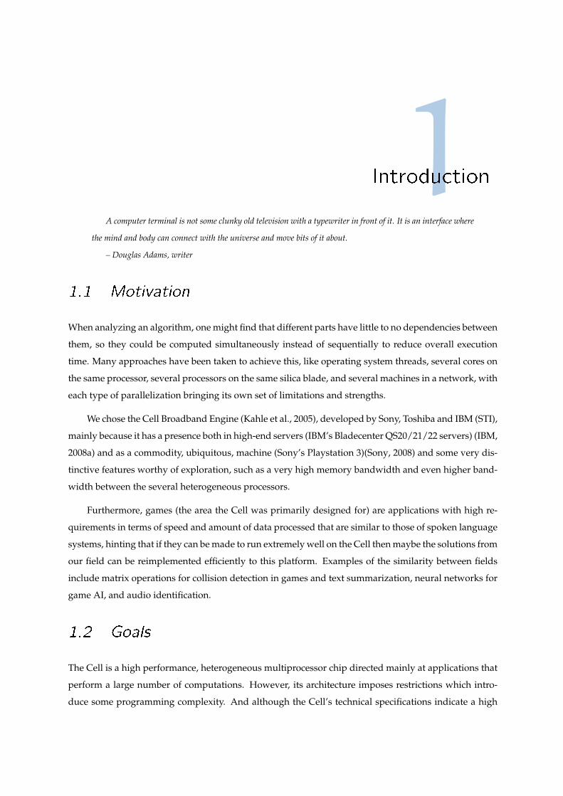
1.1 Motivation

When analyzing an algorithm, one might find that different parts have little to no dependencies between

them, so they could be computed simultaneously instead of sequentially to reduce overall execution

time. Many approaches have been taken to achieve this, like operating system threads, several cores on

the same processor, several processors on the same silica blade, and several machines in a network, with

each type of parallelization bringing its own set of limitations and strengths.

We chose the Cell Broadband Engine (Kahle et al., 2005), developed by Sony, Toshiba and IBM (STI),

mainly because it has a presence both in high-end servers (IBM’s Bladecenter QS20/21/22 servers) (IBM,

2008a) and as a commodity, ubiquitous, machine (Sony’s Playstation 3)(Sony, 2008) and some very dis-

tinctive features worthy of exploration, such as a very high memory bandwidth and even higher band-

width between the several heterogeneous processors.

Furthermore, games (the area the Cell was primarily designed for) are applications with high re-

quirements in terms of speed and amount of data processed that are similar to those of spoken language

systems, hinting that if they can be made to run extremely well on the Cell then maybe the solutions from

our field can be reimplemented efficiently to this platform. Examples of the similarity between fields

include matrix operations for collision detection in games and text summarization, neural networks for

game AI, and audio identification.

1.2 Goals

The Cell is a high performance, heterogeneous multiprocessor chip directed mainly at applications that

perform a large number of computations. However, its architecture imposes restrictions which intro-

duce some programming complexity. And although the Cell’s technical specifications indicate a high

execution speed, there are several multiprocessor high performance alternatives that must also be con-

sidered.

Therefore, this work intends to investigate the performance and usefulness of the Cell in the field of

natural language processing, providing comparisons to other platforms, while at the same time consid-

ering the programming effort needed to attain gains in execution speed. From case studies implemented

on this architecture, conclusions will be drawn with respect to what kind of problem types perform well

on the Cell, since not all cases justify the development effort needed to implement optimized applica-

tions for this processor.

These cases will provide an evaluation both from the programmer’s perspective, which can design

and implement code optimized for the Cell, and the user, which will use prebuilt, partially optimized,

libraries to obtain performance gains.

For each use case there will also be comparison metrics taken with the same (or comparable) prob-

lem implemented in at least one of current multiprocessor architectures, either processors using Intel

x86 architecture (homogeneous) or Graphics Processing Units (heterogeneous).

1.3 Structure of the Document

In chapter 2 the Cell is described, followed by chapter 3 with its most popular SDKs and frameworks;

the architecture and optimization strategies used in the implementation of the applications are explained

in chapter 4; chapter 5 contains an analysis of the performance of these case studies and comparisons

with similar implementations on other platforms; finally, this work’s conclusions, its contributions, and

future work are presented in chapter 6.

2

2The Cell Broadband

Engine Essentials

After growing wildly for years, the field of computing appears to be reaching its infancy.

– John Pierce

2.1 Introduction

This chapter introduces the concept of Single Instruction Multiple Data computing and describes the

Cell Broadband Engine, providing a basis for the following chapters.

2.2 Single Instruction Multiple Data

A vector is a data type containing a set of data elements packed in a one-dimensional array. In the

Cell these arrays are 128-bit long and support fixed-point and floating-point values. By operating on

all the elements of one vector simultaneously, e.g. four integers at a time, Single Instruction Multiple

Data (SIMD) instructions perform Data-level parallelism, introducing performance gains. This type of

computation, however, requires the program to explore these functionalities by organizing the data as

well as the computation in such a way that SIMD operations can be used.

The process of preparing a program to use SIMD operations is called SIMDization, and can be done

manually by the programmer or by a compiler/tool that performs auto-SIMDization.

SIMD instructions are abundant on the Cell, as we will see ahead. The processor supports the

vector concept both in the arithmetic processing units, operating on the 128-bit arrays, and in memory

organization, with register files of 128 registers of 128 bits each.

2.3 The Cell Broadband Engine

The Cell Broadband Engine Architecture (CBEA), of which the Cell Broadband Engine (Cell) is the first

implementation, is a definition of an architecture directed at compute-intensive applications.

The main components in the Cell are its Power Processing Element (PPE), eight Synergistic Pro-

cessing Elements (SPE - six in the Playstation 3), a Rambus XDR (Rambus, 2008) controller (MIC) that

3

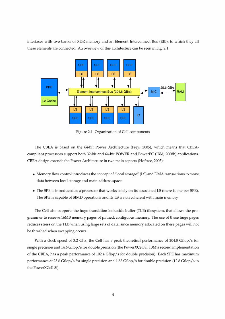
interfaces with two banks of XDR memory and an Element Interconnect Bus (EIB), to which they all

these elements are connected. An overview of this architecture can be seen in Fig. 2.1.

Element Interconnect Bus (204.8 GB/s)

SPE

LS

SPE

LS

SPE

LS

SPE

LS

SPE

LS

SPE

LS

SPE

LS

SPE

LS

PPE

L2 Cache

IO

MIC RAM25.6 GB/s

Figure 2.1: Organization of Cell components

The CBEA is based on the 64-bit Power Architecture (Frey, 2005), which means that CBEA-

compliant processors support both 32-bit and 64-bit POWER and PowerPC (IBM, 2008b) applications.

CBEA design extends the Power Architecture in two main aspects (Hofstee, 2005):

• Memory flow control introduces the concept of “local storage” (LS) and DMA transactions to move

data between local storage and main address space

• The SPE is introduced as a processor that works solely on its associated LS (there is one per SPE).

The SPE is capable of SIMD operations and its LS is non coherent with main memory

The Cell also supports the huge translation lookaside buffer (TLB) filesystem, that allows the pro-

grammer to reserve 16MB memory pages of pinned, contiguous memory. The use of these huge pages

reduces stress on the TLB when using large sets of data, since memory allocated on these pages will not

be thrashed when swapping occurs.

With a clock speed of 3.2 Ghz, the Cell has a peak theoretical performance of 204.8 Gflop/s for

single precision and 14.6 Gflop/s for double precision (the PowerXCell 8i, IBM’s second implementation

of the CBEA, has a peak performance of 102.4 Gflop/s for double precision). Each SPE has maximum

performance at 25.6 Gflop/s for single precision and 1.83 Gflop/s for double precision (12.8 Gflop/s in

the PowerXCell 8i).

4

2.3.1 Power Processing Element

The Power Processing Element is a dual-threaded 64-bit RISC processor (May et al., 1994; Tabak, 1986)

with vector/SIMD extensions. The PPE is a general purpose CPU, and is responsible on the Cell for

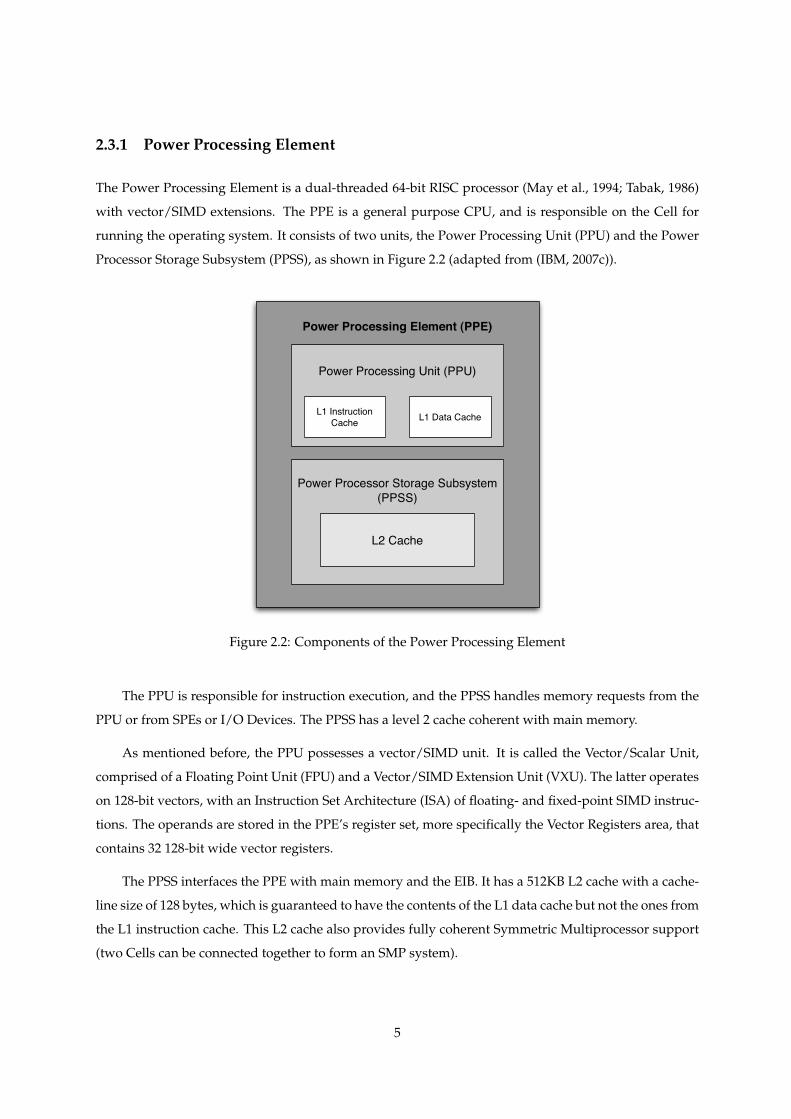
running the operating system. It consists of two units, the Power Processing Unit (PPU) and the Power

Processor Storage Subsystem (PPSS), as shown in Figure 2.2 (adapted from (IBM, 2007c)).

Power Processor Storage Subsystem (PPSS)

L2 Cache

Power Processing Element (PPE)

Power Processing Unit (PPU)

L1 Instruction Cache L1 Data Cache

Figure 2.2: Components of the Power Processing Element

The PPU is responsible for instruction execution, and the PPSS handles memory requests from the

PPU or from SPEs or I/O Devices. The PPSS has a level 2 cache coherent with main memory.

As mentioned before, the PPU possesses a vector/SIMD unit. It is called the Vector/Scalar Unit,

comprised of a Floating Point Unit (FPU) and a Vector/SIMD Extension Unit (VXU). The latter operates

on 128-bit vectors, with an Instruction Set Architecture (ISA) of floating- and fixed-point SIMD instruc-

tions. The operands are stored in the PPE’s register set, more specifically the Vector Registers area, that

contains 32 128-bit wide vector registers.

The PPSS interfaces the PPE with main memory and the EIB. It has a 512KB L2 cache with a cache-

line size of 128 bytes, which is guaranteed to have the contents of the L1 data cache but not the ones from

the L1 instruction cache. This L2 cache also provides fully coherent Symmetric Multiprocessor support

(two Cells can be connected together to form an SMP system).

5

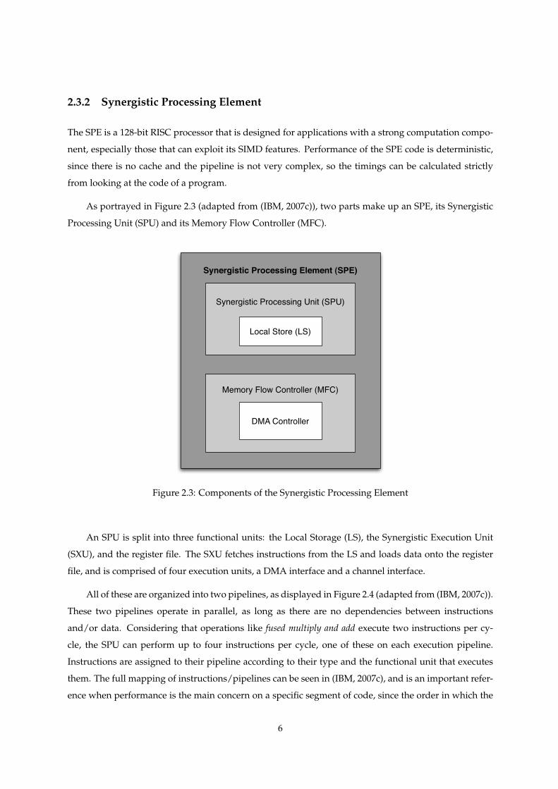
2.3.2 Synergistic Processing Element

The SPE is a 128-bit RISC processor that is designed for applications with a strong computation compo-

nent, especially those that can exploit its SIMD features. Performance of the SPE code is deterministic,

since there is no cache and the pipeline is not very complex, so the timings can be calculated strictly

from looking at the code of a program.

As portrayed in Figure 2.3 (adapted from (IBM, 2007c)), two parts make up an SPE, its Synergistic

Processing Unit (SPU) and its Memory Flow Controller (MFC).

Memory Flow Controller (MFC)

DMA Controller

Synergistic Processing Element (SPE)

Synergistic Processing Unit (SPU)

Local Store (LS)

Figure 2.3: Components of the Synergistic Processing Element

An SPU is split into three functional units: the Local Storage (LS), the Synergistic Execution Unit

(SXU), and the register file. The SXU fetches instructions from the LS and loads data onto the register

file, and is comprised of four execution units, a DMA interface and a channel interface.

All of these are organized into two pipelines, as displayed in Figure 2.4 (adapted from (IBM, 2007c)).

These two pipelines operate in parallel, as long as there are no dependencies between instructions

and/or data. Considering that operations like fused multiply and add execute two instructions per cy-

cle, the SPU can perform up to four instructions per cycle, one of these on each execution pipeline.

Instructions are assigned to their pipeline according to their type and the functional unit that executes

them. The full mapping of instructions/pipelines can be seen in (IBM, 2007c), and is an important refer-

ence when performance is the main concern on a specific segment of code, since the order in which the

6

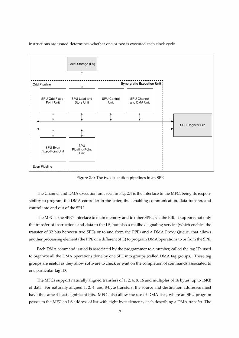
instructions are issued determines whether one or two is executed each clock cycle.

Synergistic Execution Unit

SPU Odd Fixed-Point Unit

SPU Load and Store Unit

Local Storage (LS)

SPU Control Unit

SPU Channel and DMA Unit

SPU Even Fixed-Point Unit

SPUFloating-Point

Unit

SPU Register File

Odd Pipeline

Even Pipeline

Figure 2.4: The two execution pipelines in an SPE

The Channel and DMA execution unit seen in Fig. 2.4 is the interface to the MFC, being its respon-

sibility to program the DMA controller in the latter, thus enabling communication, data transfer, and

control into and out of the SPU.

The MFC is the SPE’s interface to main memory and to other SPEs, via the EIB. It supports not only

the transfer of instructions and data to the LS, but also a mailbox signaling service (which enables the

transfer of 32 bits between two SPEs or to and from the PPE) and a DMA Proxy Queue, that allows

another processing element (the PPE or a different SPE) to program DMA operations to or from the SPE.

Each DMA command issued is associated by the programmer to a number, called the tag ID, used

to organize all the DMA operations done by one SPE into groups (called DMA tag groups). These tag

groups are useful as they allow software to check or wait on the completion of commands associated to

one particular tag ID.

The MFCs support naturally aligned transfers of 1, 2, 4, 8, 16 and multiples of 16 bytes, up to 16KB

of data. For naturally aligned 1, 2, 4, and 8-byte transfers, the source and destination addresses must

have the same 4 least significant bits. MFCs also allow the use of DMA lists, where an SPU program

passes to the MFC an LS address of list with eight-byte elements, each describing a DMA transfer. The

7

DMA controller then issues all of the specified transfers (up to 2048 per list) while the SPU resumes

execution. Considering that the current size of an LS is 256KB and DMA lists can transfer up to 32MB

of data, even if the size of the LS increases in the near future this specification should still be valid.

Due to the existence of two distinct memory spaces, RAM and SPE local stores, context switching is

a costly operation on the Cell. When this happens, the entire local store must be copied to main memory

and replaced by the one belonging to the SPE thread that will now execute. Taking this into account,

Cell developers tend to adopt a run to completion model instead of a multithreaded concurrent one.

An aspect not detailed in Fig. 2.4 is instruction fetching. In the SPE, a mispredicted instruction fetch

causes a penalty of 18-19 clock cycles. Sometimes it is favorable to avoid branches altogether by calcu-

lating both possibilities and selecting the correct value using a native assembly instruction like shuffle,

which fills a memory position with data from two other positions according to a bit pattern defined

in a fourth location. Some compilers also provide branch hinting directives to allow the developer to

indicate the most likely branch to be taken in the decision.

2.3.3 Element Interconnect Bus

The EIB consists of four 16-byte wide data rings, two running clockwise and two counter-clockwise,

with each ring transferring 128 bytes at a time. The internal maximum bandwidth of the EIB is 96 bytes

per clock cycle, and more than one transfer can occur on each ring as long as their paths do not overlap.

The theoretical bandwidth limit is 204.8 GB/s, but it is only achieved when transfers do not overlap

(which is when several transfers can share EIB rings) and there is no other contention for resources, i.e.

the full bandwidth of each SPE/EIB link is used (25.6 GB/s) and no other requests are made to the EIB

controller.

2.3.4 NUMA

In the BladeCenter QS20 and QS21, the two Cell processors operate in a Non-Uniform Memory Archi-

tecture (or Access) paradigm – NUMA –, where each processor has its own memory bank but which are

globally accessible to SPE threads running on the machine. This allows for a single application to use

all 16 SPEs at once, but since inter-Cell memory accesses are slower than on-chip ones, the program-

mer should split the data in two and programatically use the SPE’s ID number (accessible in code) to

determine which set of data is the closest to it and work preferentially on it.

8

2.4 Summary

The Cell, an implementation of the CBEA specification, is a processor with high theoretical peak perfor-

mance. However, to use this performance fully one must take into account several hardware character-

istics, like the physical layout of the SPEs and the scheduling of instructions and their assignment to the

SPE’s pipelines. Furthermore, there are software concerns while using DMA operations, relating to data

alignment and the memory locations themselves.

9

10

3Programming Models,

Existing Frameworks and

Other Platforms

3.1 Introduction

This chapter is divided into three main sections. The first section describes the several programming

models that have been suggested for Cell programs. Some have been identified only on the Cell and

others are simply a variation of more traditional models.

The second section of this chapter presents IBM’s SDK along with other frameworks and tools

available for the Cell, taking into account their limitations and strengths.

Other high performance architectures exist with the same fundamental characteristics as the Cell:

heterogeneity, availability as affordable hardware, and with a strong suite of programming tools avail-

able. One of these architectures is CUDA, developed by graphics cards maker NVIDIA, and is intro-

duced in the third part of this chapter. This platform will also be used throughout this work to provide

a performance comparison with the Cell.

3.2 Programming Models

Adapted from the models proposed in (Kahle et al., 2005), possible programming models on the Cell

are:

Function Offload Engine (FOE) Model Here the SPEs are viewed as accelerators for the main appli-

cation which executes on the PPE. Performance-critical parts of the code are offloaded to the

synergistic processors, either explicitly or via user-coded stubs, in a fashion similar to a remote

procedure call. This is the quickest way to port an existing application to the Cell, as it allows

programmers to use the SPEs computational power with small changes to the control flow of the

application.

Device-Extension Model An extension to the function offload model, where the SPEs act as front-ends

for I/O devices (which are memory-mapped on the Cell). Since the SPE’s DMA functionalities al-

low for the transfer of a single byte and for asynchronous communication via the mailbox system,

they can interact with I/O devices and appear to the PPE as one. Example applications of this

model include decrypting/encrypting all reads/writes made to the disk via the SPE virtual device.

11

Computation-Acceleration Model This is a smaller-grained model that regards the PPE only as a con-

trol processor and most, if not all, computation-intensive parts are moved to the SPEs. This model

increases the programmer’s responsibilities, as it requires the data to be manually partitioned for

the SPE tasks (some compilers may help in creating this partition).

Streaming Model Stream processing is a technique that relies on a serial or parallel pipeline of various

computational kernels and a continuous flow of data moving from one stage of the pipeline to

the next. This model is being used profusely in Graphics Processing Units programming (Buck et

al., 2004), as these processors usually have a high number of processor cores, each with a limited

instruction set, and high memory bandwidth. In the Cell, the PPE is regarded as a stream con-

troller and the SPEs act like processing kernels, using inter-SPE DMA operations to move the data

through the pipeline.

Shared Memory Multiprocessor Model Since all DMA operations in the SPEs are cache-coherent, it is

possible to regard the Cell as a shared-memory multiprocessor with two different instruction sets.

In the SPEs, standard memory loads are replaced with DMA transfers from memory to the local

store and from the local store to the register file, and memory stores correspond to the inverse

operations.

Asymmetric Thread Runtime Model This is a very popular model on symmetrical multiprocessor en-

vironments, where threads are assigned to processors by a scheduling policy that optimizes per-

formance. On the Cell there are two restrictions that have to be taken into account. First, there are

two substantially different instruction sets on the processor, so different task models must be cre-

ated for the PPE and the SPEs. Second, context switches must be avoided by scheduling policies

(as mentioned in section 2.3.2)

User Mode Thread Model This model refers to one SPE thread managing a set of user-level functions

(microthreads) running in parallel, created and supported by user software (the SPE thread is sup-

ported by the operating system). The SPE thread schedules the microthreads in shared memory,

and they span across available SPUs.

3.3 Available Frameworks

Having presented some paradigms to approach Cell programming, we now list some of the available

frameworks for this platform. In some cases, the framework matches almost exclusively one of the

models presented above. Others, however, are not limitative in that aspect and leave that decision to the

programmer. Such is the case of the first framework, IBM’s Cell SDK for Linux.

12

3.3.1 IBM Cell SDK and Simulator

IBM has developed, since the release of the Cell processor, an SDK that supports the C, C++, and Fortran

languages. It consists of header files that provide access to assembly-level functionality in DMA and

SIMD operations, along with a suite of compilers and libraries.

These libraries include mathematical functions (BLAS for matrix operations, MASS for general func-

tions like sin and square root), communication and synchronization helpers (DaCS (IBM, 2007d)) and a

SPE runtime management API for the PPE.

Another library worth considering is the Accelerated Library Framework (ALF) (IBM, 2007a), de-

signed to be integrated with the Eclipse IDE and that provides a wizard-like interface for the data parti-

tioning and overall application, generating code in the process.

Also available is a graphical full-system Cell simulator, codename Mambo (IBM, 2007e), that can

emulate a full-fledged Cell processor, including all of the PPE, SPEs, memory, disk, network and console,

in a functional simulation mode. It can also be used in performance simulation mode to obtain exact timings

for applications when developers have no access to Cell processors.

Mambo has an extensible configuration, so other types of simulations can be configured, including

a Cell Blade with two Cell processors and, to some extent, the new PowerXCell 8i SPEs IBM has recently

announced which are fully pipelined and have enhanced double precision capabilities.

The IBM SDK provides very powerful low-level access to the Cell’s potential, since most of the

interface provided consists of intrinsic functions, meaning that they map one-to-one with assembly

instructions. The experienced programmer finds in these intrinsics the tools to fine-tune and thoroughly

optimize the code. The novice user, however, will have longer development and testing times than in

more traditional computational platforms.

3.3.2 IBM XL Multicore Acceleration for Linux V0.9

The XL is a common name for IBM compilers, available for most of the hardware architectures they sell.

For the Cell, they have implemented a commercial version (IBM, 2007f) for Fortran, C, and C++. It has

two main features, automatic code SIMDization and single source automatic generation of SPE and PPE

code.

Regarding optimization, this compiler employs standard SIMDization techniques, like converting

loops to SIMD operations (Eichenberger et al., 2006), and combines them with more advanced algo-

rithms to take into account the critical path in the instruction pipeline and the dual issue capabilities of

the processor. Optimization methods also include branch prediction since branch misses are, as men-

tioned before, expensive operations on the Cell.

13

The XL Multicore Acceleration V0.9 also includes the Toronto Portable Optimizer (TPO), which pro-

vides inter- and intra-procedural optimizations. If the programmer conforms to the OpenMP (OpenMP,

2008) programming model, assuming, therefore, a single shared-memory address space, then the TPO

will look for and identify parallelizable tasks and generate the PPE and SPE executables from a single

source file. The result will be a master control thread executing on the PPE which will, with the assis-

tance of the runtime library, distribute work to the SPEs (applying the Function Offload Model or the

Computation-Acceleration Model, depending on the responsibilities assigned to the PPE).

Although this compiler is still in a development phase, it has the advantage of enabling the user to

optimize his code where he has the skill to do it and rely on XL to improve performance on the rest of

the application.

3.3.3 CorePy

CorePy (Mueller, 2007) is a Python (Python, 2008) library to explore synthetic programming on the Cell

platform. Synthetic programming consists of transforming (synthesizing) high-level code, usually in

a scripting language, into a high-performance computational kernel. This project, in particular, com-

bines low-level code with a high-productivity interpreted language, enabling the developer to produce

applications in a short time whilst still exploring the computational performance of this processor.

In the CorePy environment, the developer is exposed to the synergistic processing units (SPU) in-

struction set as a module containing native Python functions, along with other common components.

These functions are analogous to the IBM SDK’s intrinsics, since they map one-to-one with the SPU’s

assembly instruction set. There are four main modules inside the CorePy library:

ISAs are the instruction sets for the architectures CorePy supports.

InstructionStreams are wrappers for synthetic programs, i.e., containers for sequences of low-level

instructions that manage the specific tasks needed to execute them.

Processors are the executors of the synthetic programs, either synchronously or asynchronously (the

latter provide real multithreaded execution).

Memory Classes provide support for describing memory and moving data across memory boundaries.

In addition to these components, as previously mentioned, some prebuilt items exist. These include,

in the Iterators package, optimized loops using standard techniques. The Variable library has data types

with C-like semantics but optimized operators. Finally, the Expressions package is essentially syntactic

sugar for the low-level instructions available in the ISAs to make the programming task easier.

14

Programs written with CorePy can interact with any other data available to the Python interpreter,

so it is possible to use synthetic programs along with other Python libraries.

3.3.4 MPI Microtask

Message Passing is a form of parallel programming that assumes three characteristics. First, the pro-

grams are in a “nothing shared” environment, i.e., they have independent memory spaces; second, all

communication is made through a set of available message forms, transmitted generally in an asyn-

chronous fashion and finally, data transfer between files requires cooperative operations, in the sense

that for every send operation a matching recieve must be executed.

One message passing specification is the Message Passing Interface (MPI) (MPI, 2008). It is a defi-

nition of an interface that has become a de facto standard in cluster computing. There are some aspects

in which MPI extends the original message passing model, as in its second version (MPI-2) (Al Geist et

al., 1996) some interfaces are defined for sharing memory between processes.

The model enables language-independent functionality, meaning that different participants in a

cluster can be implemented in different languages, as long as they conform to the message formats.

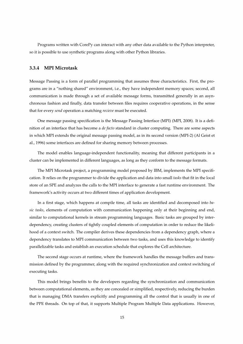
The MPI Microtask project, a programming model proposed by IBM, implements the MPI specifi-

cation. It relies on the programmer to divide the application and data into small tasks that fit in the local

store of an SPE and analyzes the calls to the MPI interface to generate a fast runtime environment. The

framework’s activity occurs at two different times of application development.

In a first stage, which happens at compile time, all tasks are identified and decomposed into ba-

sic tasks, elements of computation with communication happening only at their beginning and end,

similar to computational kernels in stream programming languages. Basic tasks are grouped by inter-

dependency, creating clusters of tightly coupled elements of computation in order to reduce the likeli-

hood of a context switch. The compiler derives these dependencies from a dependency graph, where a

dependency translates to MPI communication between two tasks, and uses this knowledge to identify

parallelizable tasks and establish an execution schedule that explores the Cell architecture.

The second stage occurs at runtime, where the framework handles the message buffers and trans-

mission defined by the programmer, along with the required synchronization and context switching of

executing tasks.

This model brings benefits to the developers regarding the synchronization and communication

between computational elements, as they are concealed or simplified, respectively, reducing the burden

that is managing DMA transfers explicitly and programming all the control that is usually in one of

the PPE threads. On top of that, it supports Multiple Program Multiple Data applications. However,

15

there are still some drawbacks in using this tool (at least in its current version). The main issue is

that it is still the programmers’ responsibility to clearly define the microtasks in the application and,

more importantly, their dependencies. The preprocessor is not yet mature enough to do these tasks

automatically.

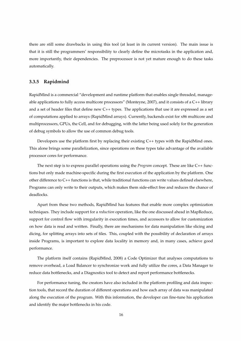
3.3.5 Rapidmind

RapidMind is a commercial “development and runtime platform that enables single threaded, manage-

able applications to fully access multicore processors” (Monteyne, 2007), and it consists of a C++ library

and a set of header files that define new C++ types. The applications that use it are expressed as a set

of computations applied to arrays (RapidMind arrays). Currently, backends exist for x86 multicore and

multiprocessors, GPUs, the Cell, and for debugging, with the latter being used solely for the generation

of debug symbols to allow the use of common debug tools.

Developers use the platform first by replacing their existing C++ types with the RapidMind ones.

This alone brings some parallelization, since operations on these types take advantage of the available

processor cores for performance.

The next step is to express parallel operations using the Program concept. These are like C++ func-

tions but only made machine-specific during the first execution of the application by the platform. One

other difference to C++ functions is that, while traditional functions can write values defined elsewhere,

Programs can only write to their outputs, which makes them side-effect free and reduces the chance of

deadlocks.

Apart from these two methods, RapidMind has features that enable more complex optimization

techniques. They include support for a reduction operation, like the one discussed ahead in MapReduce,

support for control flow with irregularity in execution times, and accessors to allow for customization

on how data is read and written. Finally, there are mechanisms for data manipulation like slicing and

dicing, for splitting arrays into sets of tiles. This, coupled with the possibility of declaration of arrays

inside Programs, is important to explore data locality in memory and, in many cases, achieve good

performance.

The platform itself contains (RapidMind, 2008) a Code Optimizer that analyses computations to

remove overhead, a Load Balancer to synchronize work and fully utilize the cores, a Data Manager to

reduce data bottlenecks, and a Diagnostics tool to detect and report performance bottlenecks.

For performance tuning, the creators have also included in the platform profiling and data inspec-

tion tools, that record the duration of different operations and how each array of data was manipulated

along the execution of the program. With this information, the developer can fine-tune his application

and identify the major bottlenecks in his code.

16

Results published (Monteyne, 2007) by the RapidMind team indicate that the tool enhances perfor-

mance on each processing element and fully uses the multiprocessor environment as a whole. However,

and as expected since it favors programability over performance, the platform loses in a comparison

with algorithms implemented with the low level frameworks available for that specific platform. On

the other hand, low level code is inherently less portable and more cumbersome to develop. RapidMind

seems very easy to use and we find particularly attractive that algorithms, when ported to this platform,

are kept conceptually serial, instead of explicitly parallel like in other frameworks.

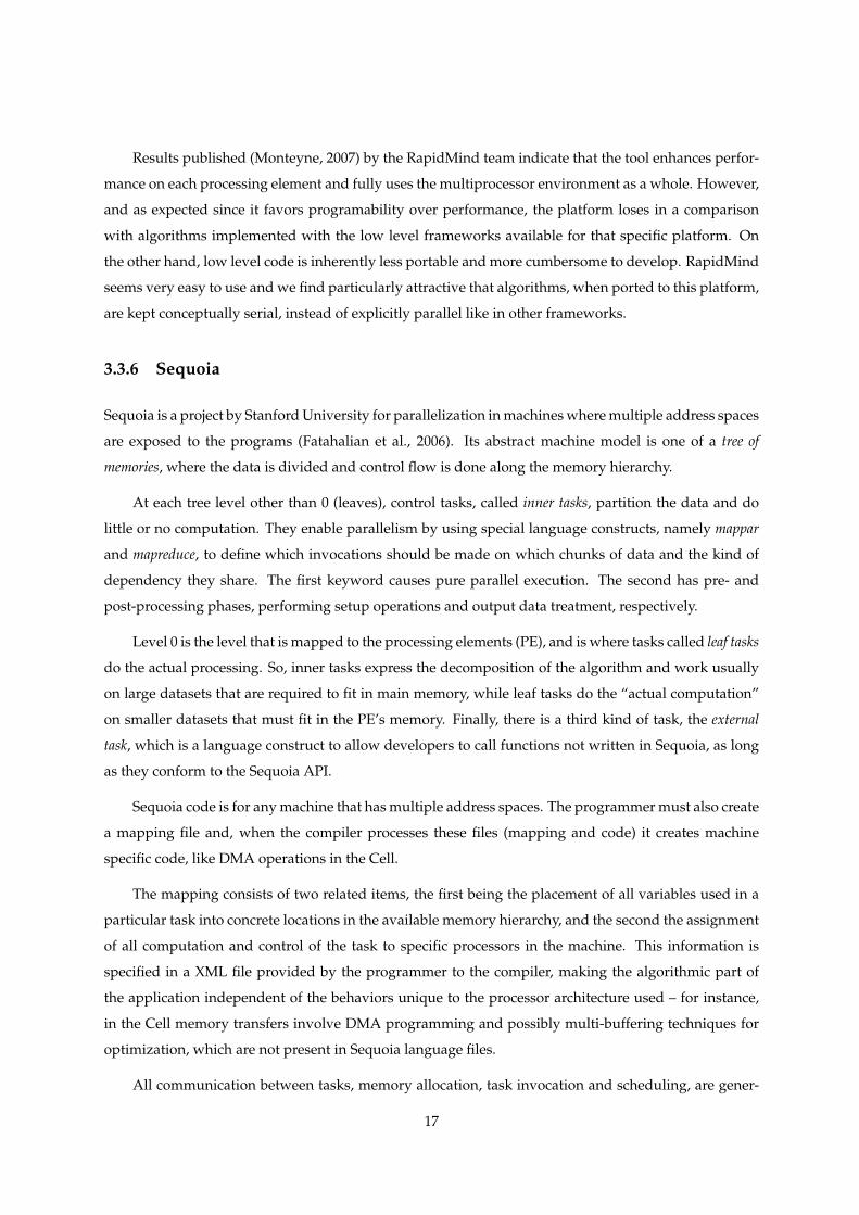
3.3.6 Sequoia

Sequoia is a project by Stanford University for parallelization in machines where multiple address spaces

are exposed to the programs (Fatahalian et al., 2006). Its abstract machine model is one of a tree of

memories, where the data is divided and control flow is done along the memory hierarchy.

At each tree level other than 0 (leaves), control tasks, called inner tasks, partition the data and do

little or no computation. They enable parallelism by using special language constructs, namely mappar

and mapreduce, to define which invocations should be made on which chunks of data and the kind of

dependency they share. The first keyword causes pure parallel execution. The second has pre- and

post-processing phases, performing setup operations and output data treatment, respectively.

Level 0 is the level that is mapped to the processing elements (PE), and is where tasks called leaf tasks

do the actual processing. So, inner tasks express the decomposition of the algorithm and work usually

on large datasets that are required to fit in main memory, while leaf tasks do the “actual computation”

on smaller datasets that must fit in the PE’s memory. Finally, there is a third kind of task, the external

task, which is a language construct to allow developers to call functions not written in Sequoia, as long

as they conform to the Sequoia API.

Sequoia code is for any machine that has multiple address spaces. The programmer must also create

a mapping file and, when the compiler processes these files (mapping and code) it creates machine

specific code, like DMA operations in the Cell.

The mapping consists of two related items, the first being the placement of all variables used in a

particular task into concrete locations in the available memory hierarchy, and the second the assignment

of all computation and control of the task to specific processors in the machine. This information is

specified in a XML file provided by the programmer to the compiler, making the algorithmic part of

the application independent of the behaviors unique to the processor architecture used – for instance,

in the Cell memory transfers involve DMA programming and possibly multi-buffering techniques for

optimization, which are not present in Sequoia language files.

All communication between tasks, memory allocation, task invocation and scheduling, are gener-

17

ated by the compiler, depending on the architecture specified in the XML file, and, in the particular case

of the Cell processor, techniques like double buffering are used to optimize performance.

Sequoia is best suited for data-centric algorithms, and the mapping of tasks to levels can be cum-

bersome in large projects as an unexperienced programmer might not be able to identify the most high-

performing mapping.

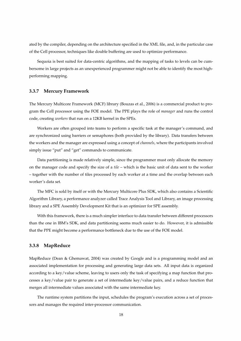
3.3.7 Mercury Framework

The Mercury Multicore Framework (MCF) library (Bouzas et al., 2006) is a commercial product to pro-

gram the Cell processor using the FOE model. The PPE plays the role of manager and runs the control

code, creating workers that run on a 12KB kernel in the SPEs.

Workers are often grouped into teams to perform a specific task at the manager’s command, and

are synchronized using barriers or semaphores (both provided by the library). Data transfers between

the workers and the manager are expressed using a concept of channels, where the participants involved

simply issue “put” and “get” commands to communicate.

Data partitioning is made relatively simple, since the programmer must only allocate the memory

on the manager code and specify the size of a tile – which is the basic unit of data sent to the worker

– together with the number of tiles processed by each worker at a time and the overlap between each

worker’s data set.

The MFC is sold by itself or with the Mercury Multicore Plus SDK, which also contains a Scientific

Algorithm Library, a performance analyzer called Trace Analysis Tool and Library, an image processing

library and a SPE Assembly Development Kit that is an optimizer for SPE assembly.

With this framework, there is a much simpler interface to data transfer between different processors

than the one in IBM’s SDK, and data partitioning seems much easier to do. However, it is admissible

that the PPE might become a performance bottleneck due to the use of the FOE model.

3.3.8 MapReduce

MapReduce (Dean & Ghemawat, 2004) was created by Google and is a programming model and an

associated implementation for processing and generating large data sets. All input data is organized

according to a key/value scheme, leaving to users only the task of specifying a map function that pro-

cesses a key/value pair to generate a set of intermediate key/value pairs, and a reduce function that

merges all intermediate values associated with the same intermediate key.

The runtime system partitions the input, schedules the program’s execution across a set of proces-

sors and manages the required inter-processor communication.

18

Implementations on machine clusters consider network latency and machine failure are contem-

plated, but these topics are ignored on the Cell since all elements are on the same chip.

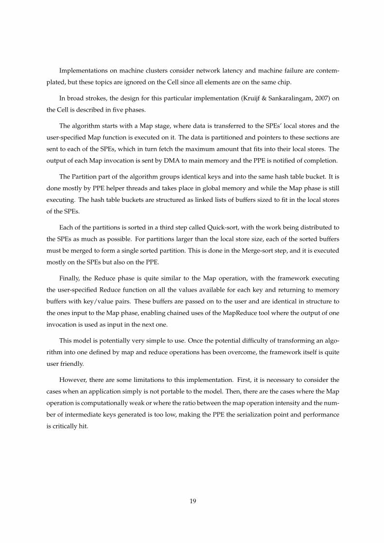
In broad strokes, the design for this particular implementation (Kruijf & Sankaralingam, 2007) on

the Cell is described in five phases.

The algorithm starts with a Map stage, where data is transferred to the SPEs’ local stores and the

user-specified Map function is executed on it. The data is partitioned and pointers to these sections are

sent to each of the SPEs, which in turn fetch the maximum amount that fits into their local stores. The

output of each Map invocation is sent by DMA to main memory and the PPE is notified of completion.

The Partition part of the algorithm groups identical keys and into the same hash table bucket. It is

done mostly by PPE helper threads and takes place in global memory and while the Map phase is still

executing. The hash table buckets are structured as linked lists of buffers sized to fit in the local stores

of the SPEs.

Each of the partitions is sorted in a third step called Quick-sort, with the work being distributed to

the SPEs as much as possible. For partitions larger than the local store size, each of the sorted buffers

must be merged to form a single sorted partition. This is done in the Merge-sort step, and it is executed

mostly on the SPEs but also on the PPE.

Finally, the Reduce phase is quite similar to the Map operation, with the framework executing

the user-specified Reduce function on all the values available for each key and returning to memory

buffers with key/value pairs. These buffers are passed on to the user and are identical in structure to

the ones input to the Map phase, enabling chained uses of the MapReduce tool where the output of one

invocation is used as input in the next one.

This model is potentially very simple to use. Once the potential difficulty of transforming an algo-

rithm into one defined by map and reduce operations has been overcome, the framework itself is quite

user friendly.

However, there are some limitations to this implementation. First, it is necessary to consider the

cases when an application simply is not portable to the model. Then, there are the cases where the Map

operation is computationally weak or where the ratio between the map operation intensity and the num-

ber of intermediate keys generated is too low, making the PPE the serialization point and performance

is critically hit.

19

3.4 Comparison

The frameworks presented have strengths and limitations, which may determine their usefulness in

solving a particular type of problem. On top of that, more generic limitations arise, like availability or

cost.

3.4.1 Programmability

RapidMind and Sequoia seem to be the favorites when it comes to programmability because they ab-

stract all of the multiprocessor characteristics from the programmer. MPI and Mercury ease commu-

nication but leave exposed the parallelism in the application, with the creation and management of

runtime elements. Furthermore, MPI Microtask and IBM XL require expertise on the MPI and OpenMP

paradigms, respectively.

MapReduce also exempts the programmer from dealing with communication and helps with mem-

ory allocation. However, it is built on top of the IBM SDK so some caveats exist, namely in memory

alignment (there are some alignment requirements for DMA operations) and performance (memory-

mapping input files, for example).

Using CorePy or the IBM SDK by themselves can be a strenuous task as they both provide only

very low-level access to the Cell.

3.4.2 Optimizations

Several of the analyzed tools, namely RapidMind, IBM XL, and Seqouia, optimize the application au-

tomatically via SIMDization, loop and memory transfer optimization techniques. MPI has automatic

optimized scheduling of SPE tasks and, like MapReduce that optimizes communication, requires the

programmer to optimize his own code.

Viewing optimization from another perspective, we notice that Rapidmind and Sequoia allow for

little to none fine-tuning, while an experienced Cell programmer using CorePy or IBM’s SDK can op-

timize at assembly level taking into account the semantic particularities of the data. The issue is how

experienced a programmer must be to out-optimize an equivalent Sequoia/RapidMind algorithm.

3.4.3 Completeness

Most of the described platforms demand the algorithm or data to conform to a specific model or be

organized a certain way. So, it may occur that a particular algorithm cannot be implemented in the

20

MapReduce paradigm, or in the OpenMP standard. Therefore the programmer that intends to use one

of these tools should first validate the applicability of these metamodels to the particular application to

implement. For example, in a project where the processing of a chunk of information depends on “adja-

cent” data, the MapReduce algorithm may be hard to apply since each unit is processed independently.

3.4.4 Commercial and Maturity Issues

Apart from the previous points, issues like the availability and maturity of these frameworks are very

relevant. For instance RapidMind, although a very attractive platform, is prohibitively expensive and

will not be further investigated, and Sequoia shows several shortcomings since some important lan-

guage constructs remain unimplemented.

MapReduce development has ceased (but some support exists) and, although some changes that

would bring much better performance have been identified, they will not be implemented in the near

future. Also, MPI Microtask is not available to the public, as only a simple prototype has been imple-

mented as proof of concept. Finally, some tools are only compatible with the IBM SDK version 2.1,

which may cause some limitations to users who wish to take advantage of newer features.

3.5 CUDA by NVIDIA

NVIDIA, a graphics card maker, has created a development platform to leverage the power of their

GPUs in general-purpose (i.e. not just graphics-related) applications. Compute Unified Device Archi-

tecture (CUDA) is suite of compiler and tools to enable developers to code algorithms in a streaming

model and deploy them in recent GPUs. The NVIDIA GPU GeForce 8800GTX, which supports CUDA,

is organized into 16 Streaming Multiprocessors (SM), each with 8 processing units, with a global theo-

retical peak performance of 345.6 GFLOPS for single precision data. All these processing units are, like

the Cell SPEs, SIMD-capable and, also like what happens with the Cell, have much higher performance

on single precision floating point operands than with double precision. This graphics card was available

for testing, so it was used to provide comparative data.

To use CUDA, the developer allocates memory on the device and copies the data to those locations.

Then, he runs GPU threads, which then execute (usually small) computational kernels on the data in

parallel (NVIDIA, 2008). Only one particular kernel can be executed by a device at a given time, but

many instances of that same kernel can run simultaneously on different data.

CUDA provides simple extensions to C language in the form of annotations to distinguish between

GPU and CPU code, along with functions to manage the memory allocation and transfer between host

(CPU) and guest (GPU) devices. To define a computacional kernel, the programmer annotates a C

21

function with the global declaration specifier and to invoke it the syntax element ≪ ... ≫ is added

to the function name with two arguments, specifying the organization of the work into threads in blocks

and of blocks in the grid respectively (see below).

In CUDA, a block is a group of worker threads conceptually organized in a 1-, 2- or 3-dimensional

space. All threads within a block can use shared memory and synchronization mechanisms to cooperate

among themselves. Blocks are also organized in a 1-dimensional or 2-dimensional space called a grid.

However, unlike the threads in one block, all blocks in a grid must be completely independent from

each other, since they can be executed in any order.

Apart from these language extensions, the CUDA platform defines, to take advantage of the SIMD

features of the processors, vector data types with 1, 2, 3 and 4 dimensions. For example, single precision

floating point types float1, float2, float3 and float4 are defined, and each scalar in the vector can be accessed

using notation similar to C structures, the 1st, 2nd, 3rd and 4th components being called x, y, z and w,

respectively.

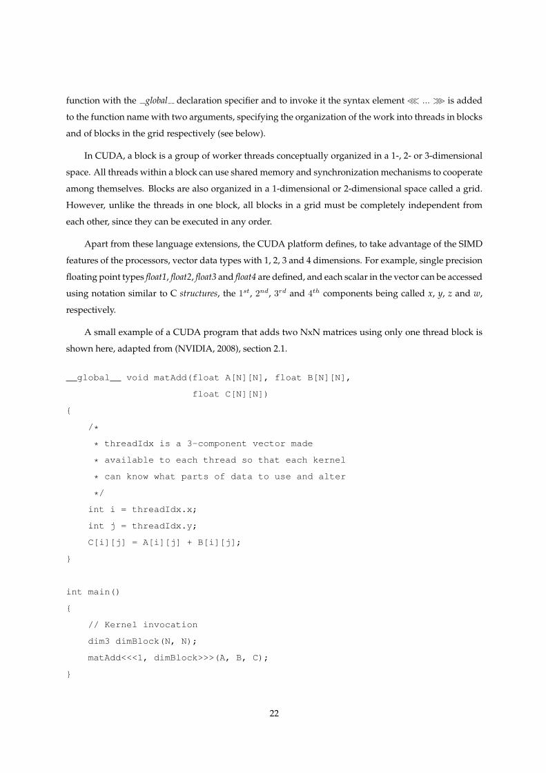
A small example of a CUDA program that adds two NxN matrices using only one thread block is

shown here, adapted from (NVIDIA, 2008), section 2.1.

__global__ void matAdd(float A[N][N], float B[N][N],

float C[N][N])

{

/*

* threadIdx is a 3-component vector made

* available to each thread so that each kernel

* can know what parts of data to use and alter

*/

int i = threadIdx.x;

int j = threadIdx.y;

C[i][j] = A[i][j] + B[i][j];

}

int main()

{

// Kernel invocation

dim3 dimBlock(N, N);

matAdd<<<1, dimBlock>>>(A, B, C);

}

22

In this example, the thread block is a square with a side of N, and each thread in the block computes

only one position of the result matrix.

These data types can be manipulated with the usual arithmetic operators (+,−, /, ∗) but other com-

mon mathematical functions like sin, cos, tan, log and exp are only available for scalar types on the

device. However, two sets of implementations of these functions exist, one with less precision but faster

and another more accurate but slower execution.

Like the Cell and its NUMA architecture, NVIDIA’s latest products are capable of being used co-

operatively with their Scalable Link Interface (SLI) technology (NVIDIA, 2009), assuming the GPUs

are mounted on a SLI-compatable motherboard. According to NVIDIA, the SLI connectors allow for a

maximum transfer rate between cards of 1GB/s, and a maximum of 3 cards can be interconnected.

3.6 Summary

In this chapter some programming models have been presented that deal with the Cell’s heterogeneous

architecture, each proposing different roles for the PPE and SPEs according to the type of problem the

application is directed to.

The frameworks listed, in another perspective, provide more or less abstraction from the processor

itself, with some granting the programmer a more fine-grained control and low level access to the Cell

whilst others hide processor intricacies like DMA transfers and overall SPE management.

Although these frameworks are relevant, each in its problem space, they also have characteristics

that condition their applicability and availability for this work, such as their price or maturity.

In a broader perspective of parallel heterogeneous processors, the NVIDIA CUDA suite provides

access to the computing power of modern NVIDIA GPUs and presents a high-performance computing

alternative to the Cell altogether, with apparently less programming effort than the one required to use

IBM’s SDK.

CUDA’s streaming programming model is quite easy to apply when the algorithm is based on

computation of many independent chunks of data. When the application requires more synchronization

and/or information sharing between the worker threads, greater planning has to go into the allocation

scheme of work to threads/blocks.

23

24

4Case Studies

4.1 Introduction

So far in this document, the Cell has been described both through an overview of its hardware charac-

teristics and trough its programming requirements and available tools. But to evaluate its usefulness,

especially in the natural language processing field, some common problems in the area were approached

using Cell-based solutions.

This chapter consists of a description of the applications implemented on the Cell, more precisely

their purpose, architecture, and optimizations. The first application presented was implemented in a

more naıve fashion, and the remaining two were done taking into account some optimization techniques

like loop unrolling, multibuffering, computation/data transfer overlapping, and others.

In the next chapter the performance of the implementations described here will be analyzed with

the above concerns in mind, in order to determine the degree of optimization needed to obtain signifi-

cant performance gains in relation to similar solutions on other platforms.

4.2 Neural Networks

Neural networks (Jain et al., 1996) are a tool that is frequently used in the field of natural language pro-

cessing. One example is an application developed at Inesc ID, Laboratorio de Lıngua Falada (L2F) (San-

tos Meinedo, 2008), built with the purpose of identifying jingles in an audio stream to detect the begin-

ning/end of broadcast news, along with commercial breaks and filler segments.

This jingle detector consists of a pipeline of different tools. In the first step, features are extracted

from the audio stream, based on audio signal energy and other characteristics. From each sample, a

total of 26 features are extracted into a feature vector.

The resulting information is input to the second step, a neural network classifier of the type Multi-

Layer Perceptron (MLP) that classifies the feature vectors and outputs the probability of each frame

being a certain type of jingle. To increase classification accuracy, the vectors are evaluated along with a

group of adjacent samples, called context frames. The output of this step is then smoothed by a median

filter and compared to a threshold value (pre-determined).

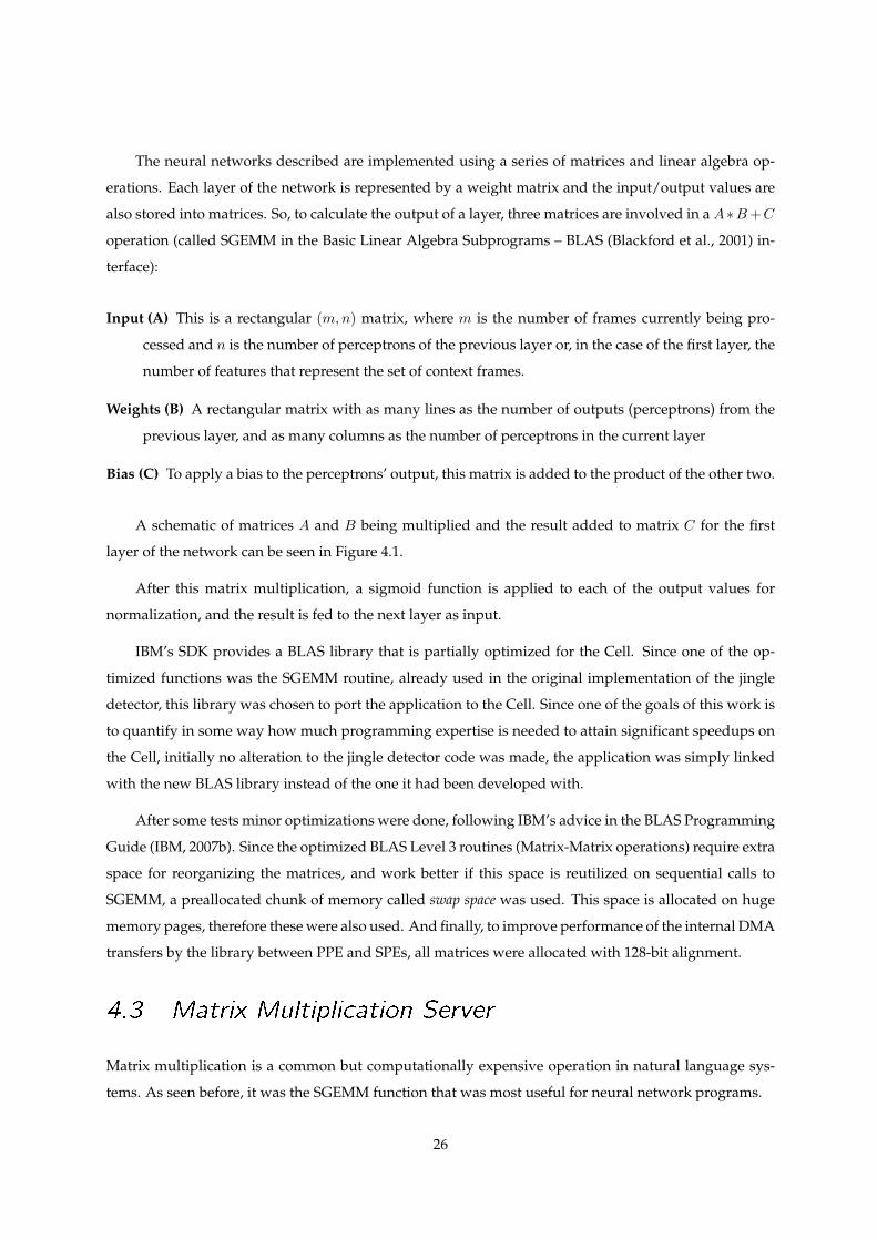
The neural networks described are implemented using a series of matrices and linear algebra op-

erations. Each layer of the network is represented by a weight matrix and the input/output values are

also stored into matrices. So, to calculate the output of a layer, three matrices are involved in a A∗B +C

operation (called SGEMM in the Basic Linear Algebra Subprograms – BLAS (Blackford et al., 2001) in-

terface):

Input (A) This is a rectangular (m, n) matrix, where m is the number of frames currently being pro-

cessed and n is the number of perceptrons of the previous layer or, in the case of the first layer, the

number of features that represent the set of context frames.

Weights (B) A rectangular matrix with as many lines as the number of outputs (perceptrons) from the

previous layer, and as many columns as the number of perceptrons in the current layer

Bias (C) To apply a bias to the perceptrons’ output, this matrix is added to the product of the other two.

A schematic of matrices A and B being multiplied and the result added to matrix C for the first

layer of the network can be seen in Figure 4.1.

After this matrix multiplication, a sigmoid function is applied to each of the output values for

normalization, and the result is fed to the next layer as input.

IBM’s SDK provides a BLAS library that is partially optimized for the Cell. Since one of the op-

timized functions was the SGEMM routine, already used in the original implementation of the jingle

detector, this library was chosen to port the application to the Cell. Since one of the goals of this work is

to quantify in some way how much programming expertise is needed to attain significant speedups on

the Cell, initially no alteration to the jingle detector code was made, the application was simply linked

with the new BLAS library instead of the one it had been developed with.

After some tests minor optimizations were done, following IBM’s advice in the BLAS Programming

Guide (IBM, 2007b). Since the optimized BLAS Level 3 routines (Matrix-Matrix operations) require extra

space for reorganizing the matrices, and work better if this space is reutilized on sequential calls to

SGEMM, a preallocated chunk of memory called swap space was used. This space is allocated on huge

memory pages, therefore these were also used. And finally, to improve performance of the internal DMA

transfers by the library between PPE and SPEs, all matrices were allocated with 128-bit alignment.

4.3 Matrix Multiplication Server

Matrix multiplication is a common but computationally expensive operation in natural language sys-

tems. As seen before, it was the SGEMM function that was most useful for neural network programs.

26

Bias Matrix

Product Matrix

Weight Matrix

No. of perceptrons in layerNo. of features per context

Laye

r Inp

ut M

atrix

No. o

f fra

mes

in b

unch

...

Perc

eptro

n 1

Perc

eptro

n 2

Perc

eptro

n N

Frame 1Frame 2

...

+2 ... N

Figure 4.1: Matrix multiplication in the first layer of the neural network

Different implementations of the operation exist in the many linear algebra libraries available, in-

cluding the IBM BLAS library provided with the Cell SDK. Having no knowledge of how this function

is implemented by IBM, we decided to investigate the performance gains of a highly optimized, low

level, version of this linear algebra operation in comparison to IBM’s BLAS.

Since the original application this case study was based on showed promising results, a choice was

made to create a server that could be invoked by code running on other platforms, using an RPC-like

communication protocol.

This section describes the architecture and optimization of the application. More precisely, it re-

ceives three matrices (A, B, and C) as input and then performs the operation A*B+C, destructively

changing matrix C. This application was based on Daniel Hackenberg’s (Hackenberg, 2008) implemen-

tation. First, the matrix multiplication code will be described; then the server part of the program.

27

4.3.1 Matrix Multiplication part

4.3.1.1 Data Organization

In this application, the input data is partitioned into square blocks of 64x64 single precision floating point

elements. These may be organized in memory in the traditional (C language) row major layout (RML)

or in block data layout (BDL). This choice influences performance, since when RML is used all DMA

operations must use the scatter/gather facilities that DMA lists provide (recall 2.3.2), while in BDL an

entire block may be transmitted in a single DMA operation (Kistler et al., 2006).

4.3.1.2 Work Partitioning

In this application, the PPE has only setup and statistics collection duties, with all the calculations being

performed on the SPEs. To improve the (calculation time)/(DMA latency) ratio, each SPE works on four

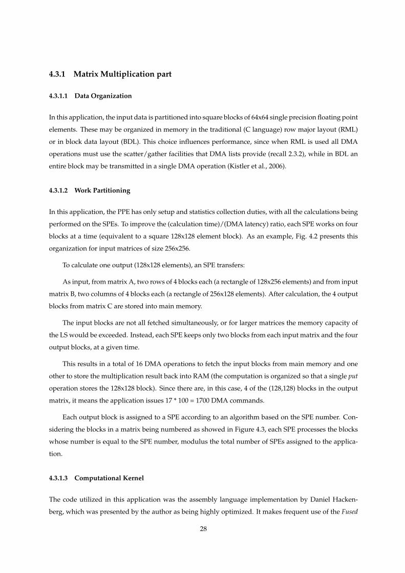
blocks at a time (equivalent to a square 128x128 element block). As an example, Fig. 4.2 presents this

organization for input matrices of size 256x256.

To calculate one output (128x128 elements), an SPE transfers:

As input, from matrix A, two rows of 4 blocks each (a rectangle of 128x256 elements) and from input

matrix B, two columns of 4 blocks each (a rectangle of 256x128 elements). After calculation, the 4 output

blocks from matrix C are stored into main memory.

The input blocks are not all fetched simultaneously, or for larger matrices the memory capacity of

the LS would be exceeded. Instead, each SPE keeps only two blocks from each input matrix and the four

output blocks, at a given time.

This results in a total of 16 DMA operations to fetch the input blocks from main memory and one

other to store the multiplication result back into RAM (the computation is organized so that a single put

operation stores the 128x128 block). Since there are, in this case, 4 of the (128,128) blocks in the output

matrix, it means the application issues 17 * 100 = 1700 DMA commands.

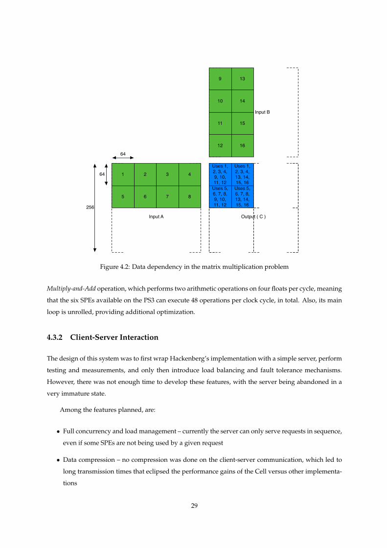
Each output block is assigned to a SPE according to an algorithm based on the SPE number. Con-

sidering the blocks in a matrix being numbered as showed in Figure 4.3, each SPE processes the blocks

whose number is equal to the SPE number, modulus the total number of SPEs assigned to the applica-

tion.

4.3.1.3 Computational Kernel

The code utilized in this application was the assembly language implementation by Daniel Hacken-

berg, which was presented by the author as being highly optimized. It makes frequent use of the Fused

28

Output ( C )

Uses 1, 2, 3, 4, 9, 10, 11, 12

Uses 5, 6, 7, 8, 9, 10, 11, 12

Uses 1, 2, 3, 4, 13, 14, 15, 16

Uses 5, 6, 7, 8, 13, 14, 15, 16

Input A

1

5

2

6

3

7

4

8

Input B

9

12

11

10

13

16

15

14

64

64

256

Figure 4.2: Data dependency in the matrix multiplication problem

Multiply-and-Add operation, which performs two arithmetic operations on four floats per cycle, meaning

that the six SPEs available on the PS3 can execute 48 operations per clock cycle, in total. Also, its main

loop is unrolled, providing additional optimization.

4.3.2 Client-Server Interaction

The design of this system was to first wrap Hackenberg’s implementation with a simple server, perform

testing and measurements, and only then introduce load balancing and fault tolerance mechanisms.

However, there was not enough time to develop these features, with the server being abandoned in a

very immature state.

Among the features planned, are:

• Full concurrency and load management – currently the server can only serve requests in sequence,

even if some SPEs are not being used by a given request

• Data compression – no compression was done on the client-server communication, which led to

long transmission times that eclipsed the performance gains of the Cell versus other implementa-

tions

29

0 1 2 3 4

5 6 7 8 9

64

64

10 11 12 13 14

15 16 17 18 19

20 21 22 23 24

Legend:

Processed by SPE 0 Processed by SPE 1 Processed by SPE 2

Figure 4.3: Work assignment to the SPEs example, using 3 SPEs and (5 ∗ 64, 5 ∗ 64) matrices

• Fault tolerance – as there was no internal state consistency check, a transmission error or client

crash would lead to a server failure.

4.4 Euclidean Distance Calculator

In the field of music analysis, various techniques have been used for information extraction (Logan, 2000;

Makhoul, 1975). At INESC-ID there is such a project, led by Prof. David Matos and Ricardo Santos, that

extracts features from songs, performs similarity detection between them, and finally groups them to

obtain information such as location and duration of choruses, openings, and similarities to other songs.

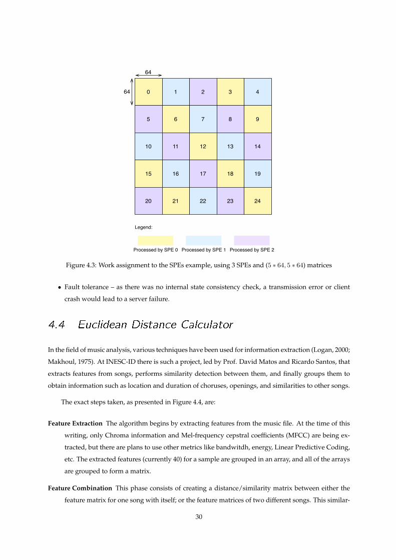
The exact steps taken, as presented in Figure 4.4, are:

Feature Extraction The algorithm begins by extracting features from the music file. At the time of this

writing, only Chroma information and Mel-frequency cepstral coefficients (MFCC) are being ex-

tracted, but there are plans to use other metrics like bandwitdh, energy, Linear Predictive Coding,

etc. The extracted features (currently 40) for a sample are grouped in an array, and all of the arrays

are grouped to form a matrix.

Feature Combination This phase consists of creating a distance/similarity matrix between either the

feature matrix for one song with itself; or the feature matrices of two different songs. This similar-

30

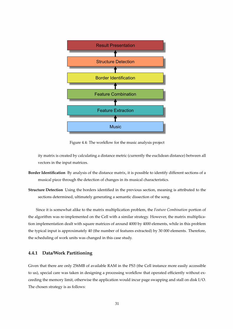
Music

Feature Extraction

Feature Combination

Border Identification

Structure Detection

Result Presentation

Figure 4.4: The workflow for the music analysis project

ity matrix is created by calculating a distance metric (currently the euclidean distance) between all

vectors in the input matrices.

Border Identification By analysis of the distance matrix, it is possible to identify different sections of a

musical piece through the detection of changes in its musical characteristics.

Structure Detection Using the borders identified in the previous section, meaning is attributed to the

sections determined, ultimately generating a semantic dissection of the song.

Since it is somewhat alike to the matrix multiplication problem, the Feature Combination portion of

the algorithm was re-implemented on the Cell with a similar strategy. However, the matrix multiplica-

tion implementation dealt with square matrices of around 4000 by 4000 elements, while in this problem

the typical input is approximately 40 (the number of features extracted) by 30 000 elements. Therefore,

the scheduling of work units was changed in this case study.

4.4.1 Data/Work Partitioning

Given that there are only 256MB of available RAM in the PS3 (the Cell instance more easily accessible

to us), special care was taken in designing a processing workflow that operated efficiently without ex-

ceeding the memory limit, otherwise the application would incur page swapping and stall on disk I/O.

The chosen strategy is as follows:

31

• The side of each square block is the number of features per sample, 40, but configurable to a

maximum of 64 (which renders a block of the maximum size allowed for a single DMA transfer)

• The input matrices are organized in BDL, with each feature vector sequentially in memory and all

the vectors also stored sequentially.

• The SPEs process areas of the matrix called “lines” that are 128 rows by m columns, where m is the

length of the side of the matrix.

• The atomic work unit for a SPE consists of four blocks from input (two from each matrix) and four

blocks to output. This is similar to what happened in the matrix multiplication application. How-

ever, in this case, the two blocks from one of the input matrices are reutilized for the processing of

the whole “line” and remain in the SPE for this entire period.

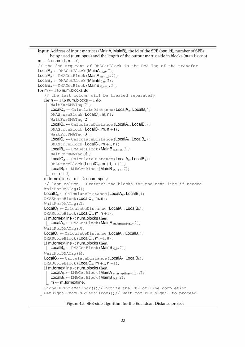
The algorithm for each SPE is presented in Figure 4.5.

When a SPE finishes a line, it must wait for PPE notification. This is because of another strategy

derived from the small memory available, where the PPE periodically flushes the output buffers to the

result file.

The PPE maintains two buffers, each large enough to hold one output line from each SPE. To reduce

the stall time when the SPEs finish one iteration and the result must be written to disk, a double buffering

technique was used. This translates into the result of one iteration being flushed while the next is being

calculated. To accommodate this, the SPEs receive two addresses for main memory output as argument,

and after each line is processed the designated output pointer is swapped. These changes are better

explained in Figure 4.6.

32

input: Address of input matrices (MainA, MainB), the id of the SPE (spe id), number of SPEsbeing used (num spes) and the length of the output matrix side in blocks (num blocks)

m← 2 ∗ spe id , n← 0;// the 2nd argument of DMAGetBlock is the DMA Tag of the transferLocalAa← DMAGetBlock(MainA m,0, 1);LocalAb← DMAGetBlock(MainA m+1,0, 1);LocalBa← DMAGetBlock(MainB 0,n, 1);LocalBb← DMAGetBlock(MainB 0,n+1, 1);for m← 1 to num blocks do

// the last column will be treated separatelyfor n← 1 to num blocks− 1 do

WaitForDMATag(1);LocalCa← CalculateDistance(LocalAa, LocalBa);DMAStoreBlock(LocalCa, m, n);WaitForDMATag(2);LocalCb← CalculateDistance(LocalAa, LocalBb);DMAStoreBlock(LocalCb, m, n +1);WaitForDMATag(3);LocalCc ← CalculateDistance(LocalAb, LocalBa);DMAStoreBlock(LocalCc, m +1, n);LocalBa← DMAGetBlock(MainB 0,n+2, 1);WaitForDMATag(4);LocalCd← CalculateDistance(LocalAb, LocalBb);DMAStoreBlock(LocalCd, m +1, n +1);LocalBb← DMAGetBlock(MainB 0,n+3, 2);n← n + 2;

m fornextline← m + 2 ∗ num spes;// last column. Prefetch the blocks for the next line if neededWaitForDMATag(1);LocalCa ← CalculateDistance(LocalAa, LocalBa);DMAStoreBlock(LocalCa, m, n);WaitForDMATag(2);LocalCb ← CalculateDistance(LocalAa, LocalBb);DMAStoreBlock(LocalCb, m, n +1);if m fornextline < num blocks then

LocalAa← DMAGetBlock(MainA m fornextline,0, 1);WaitForDMATag(3);LocalCc ← CalculateDistance(LocalAb, LocalBa);DMAStoreBlock(LocalCc, m +1, n);if m fornextline < num blocks then

LocalBa← DMAGetBlock(MainB 0,0, 1);WaitForDMATag(4);LocalCd ← CalculateDistance(LocalAb, LocalBb);DMAStoreBlock(LocalCd, m +1, n +1);if m fornextline < num blocks then

LocalAb← DMAGetBlock(MainA m fornextline+1,0, 2);LocalBb← DMAGetBlock(MainB 0,1, 2);m← m fornextline;

SignalPPEViaMailbox(); // notify the PPE of line completionGetSignalFromPPEViaMailbox(); // wait for PPE signal to proceed

Figure 4.5: SPE-side algorithm for the Euclidean Distance project

33

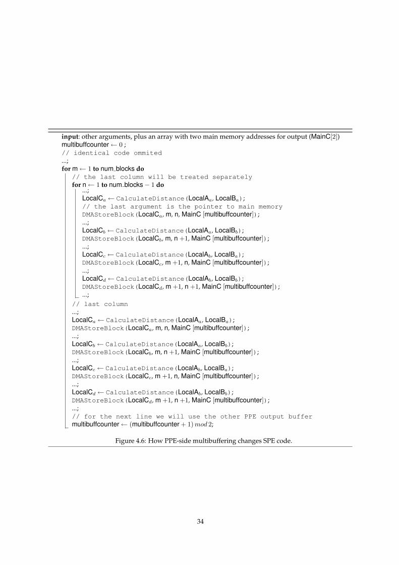
input: other arguments, plus an array with two main memory addresses for output (MainC[2])multibuffcounter← 0 ;// identical code ommited...;for m← 1 to num blocks do

// the last column will be treated separatelyfor n← 1 to num blocks− 1 do

...;LocalCa← CalculateDistance(LocalAa, LocalBa);// the last argument is the pointer to main memoryDMAStoreBlock(LocalCa, m, n, MainC [multibuffcounter]);...;LocalCb← CalculateDistance(LocalAa, LocalBb);DMAStoreBlock(LocalCb, m, n +1, MainC [multibuffcounter]);...;LocalCc ← CalculateDistance(LocalAb, LocalBa);DMAStoreBlock(LocalCc, m +1, n, MainC [multibuffcounter]);...;LocalCd← CalculateDistance(LocalAb, LocalBb);DMAStoreBlock(LocalCd, m +1, n +1, MainC [multibuffcounter]);...;

// last column...;LocalCa ← CalculateDistance(LocalAa, LocalBa);DMAStoreBlock(LocalCa, m, n, MainC [multibuffcounter]);...;LocalCb ← CalculateDistance(LocalAa, LocalBb);DMAStoreBlock(LocalCb, m, n +1, MainC [multibuffcounter]);...;LocalCc ← CalculateDistance(LocalAb, LocalBa);DMAStoreBlock(LocalCc, m +1, n, MainC [multibuffcounter]);...;LocalCd← CalculateDistance(LocalAb, LocalBb);DMAStoreBlock(LocalCd, m +1, n +1, MainC [multibuffcounter]);...;// for the next line we will use the other PPE output buffermultibuffcounter← (multibuffcounter + 1) mod 2;

Figure 4.6: How PPE-side multibuffering changes SPE code.

34

5Results and Evaluation

5.1 Introduction

This chapter consists in a description of the performance and scalability tests done on the previously

described case studies, in an attempt to ascertain what types of problems and, more specifically, the

problem dimension intervals where the programs had considerable speedups.

The results in this chapter are based on timings on a number of runs of the applications over sev-

eral platforms, and we have chosen to display them either as execution time versus data size/CPU, as

GFLOPS versus data size/CPU or as relative speedup of one platform using another as a comparison

basis.

5.2 Testing environment

In all tests, the main Cell instance used was a PS3 running the Fedora 7 operating system, with 256MB

of RAM available for the Cell of which 32MB were reserved for huge page allocations. This particular

implementation of the Cell only has 6 SPEs available to the programmer instead of the standard 8, but

in all other relevant aspects (memory bandwidth, EIB clock speed, etc.) it is identical to the BladeCenter

QS20 and QS21 versions of the processor. For the matrix multiplication case study the implementation

was also run on QS20 machines, with 1GB RAM and 16 SPEs, provided by the Georgia Tech Institute.

To provide a comparison, two other machine configurations were used. One, configuration A,

consisted of an Intel Q6600 Core2 Quad CPU, with 8GB of DDR2 RAM at 600MHz. The other machine,

configuration B, used the same processor, but with an NVIDIA 8800GT graphics card and a higher mem-

ory clock rate of 800MHz. In configuration A the BLAS library used was Intel MKL version 10.0.5.025

and, in configuration B, the tests used the cuBLAS library provided with the CUDA SDK.

5.3 Neural Networks

As explained before, this application was first ported to the Cell in a naıve fashion, replacing only the

BLAS library used in the original implementation with IBM’s version and leaving the rest of the code

unchanged.

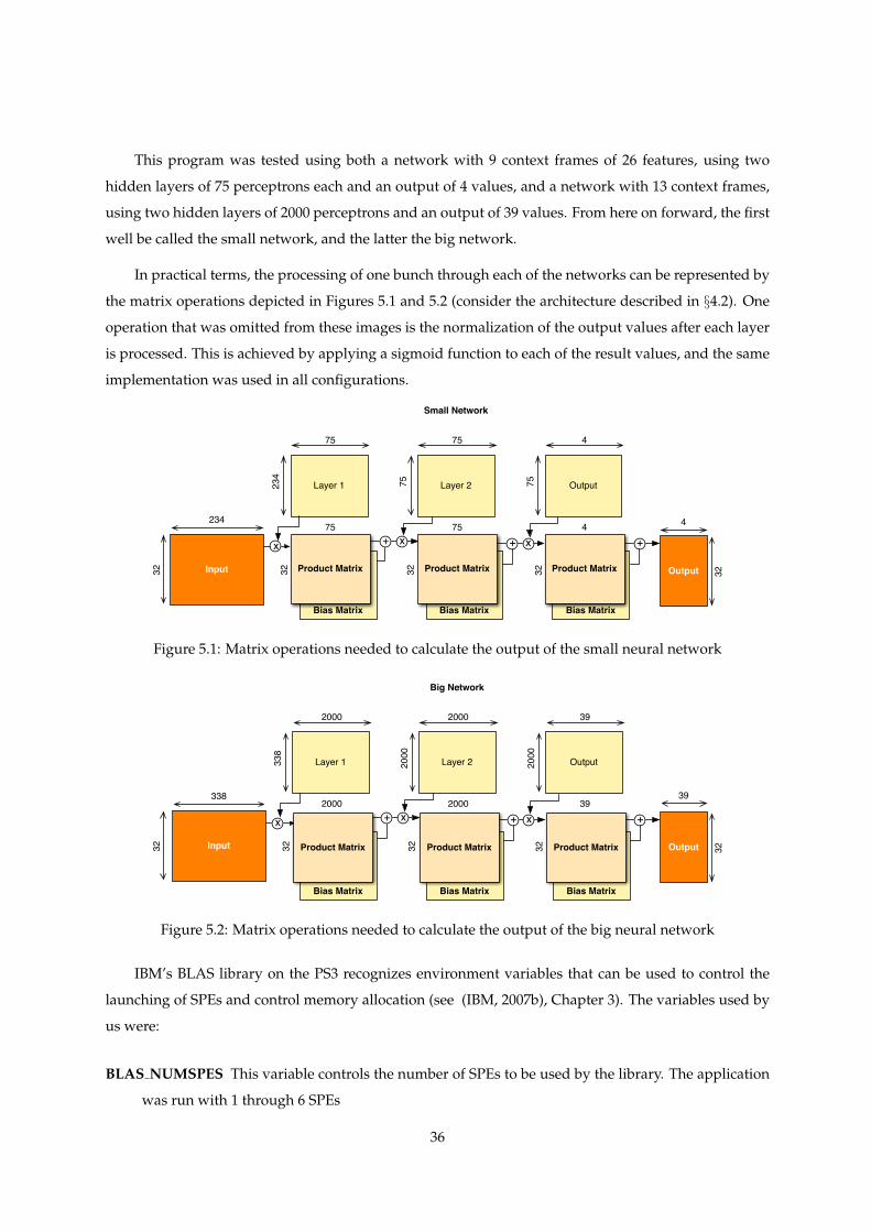
This program was tested using both a network with 9 context frames of 26 features, using two

hidden layers of 75 perceptrons each and an output of 4 values, and a network with 13 context frames,

using two hidden layers of 2000 perceptrons and an output of 39 values. From here on forward, the first

well be called the small network, and the latter the big network.

In practical terms, the processing of one bunch through each of the networks can be represented by

the matrix operations depicted in Figures 5.1 and 5.2 (consider the architecture described in §4.2). One

operation that was omitted from these images is the normalization of the output values after each layer

is processed. This is achieved by applying a sigmoid function to each of the result values, and the same

implementation was used in all configurations.

Bias Matrix

Product Matrix

Small Network

234

32

Layer 1

Input

+

234

75

Bias Matrix

Product Matrix32

Layer 275

75

75 75

Bias Matrix

Product Matrix

Output75

4

432 Output32

4

32

x x + +x

Figure 5.1: Matrix operations needed to calculate the output of the small neural network

Bias Matrix

Big Network

338

32

Layer 1

Input

+

338

2000

Bias Matrix

32

Layer 22000

2000

2000 2000

Bias Matrix

Output2000

39

39

32 Output32

39

32

x x + +x

Product Matrix Product Matrix Product Matrix

Figure 5.2: Matrix operations needed to calculate the output of the big neural network

IBM’s BLAS library on the PS3 recognizes environment variables that can be used to control the

launching of SPEs and control memory allocation (see (IBM, 2007b), Chapter 3). The variables used by

us were:

BLAS NUMSPES This variable controls the number of SPEs to be used by the library. The application

was run with 1 through 6 SPEs

36

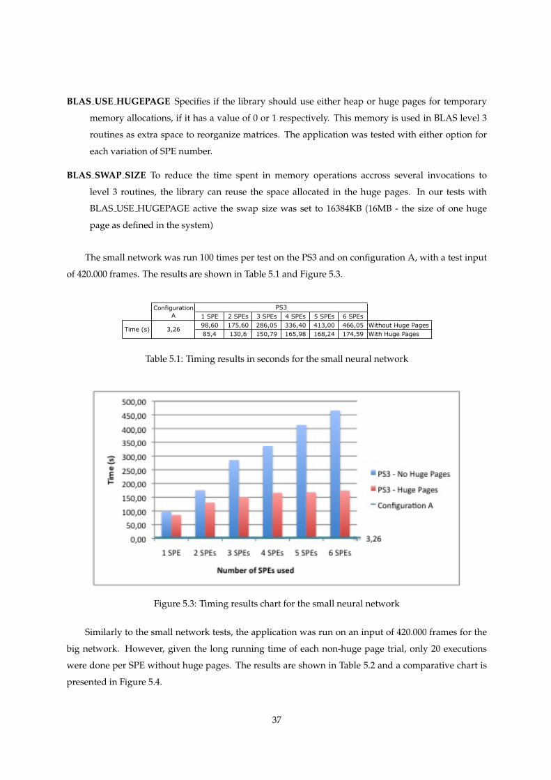
BLAS USE HUGEPAGE Specifies if the library should use either heap or huge pages for temporary

memory allocations, if it has a value of 0 or 1 respectively. This memory is used in BLAS level 3

routines as extra space to reorganize matrices. The application was tested with either option for

each variation of SPE number.

BLAS SWAP SIZE To reduce the time spent in memory operations accross several invocations to

level 3 routines, the library can reuse the space allocated in the huge pages. In our tests with

BLAS USE HUGEPAGE active the swap size was set to 16384KB (16MB - the size of one huge

page as defined in the system)

The small network was run 100 times per test on the PS3 and on configuration A, with a test input

of 420.000 frames. The results are shown in Table 5.1 and Figure 5.3.

1 SPE 2 SPEs 3 SPEs 4 SPEs 5 SPEs 6 SPEs

98,60 175,60 286,05 336,40 413,00 466,05 Without Huge Pages

85,4 130,6 150,79 165,98 168,24 174,59 With Huge Pages3,26Time (s)

PS3Configuration

A

Table 5.1: Timing results in seconds for the small neural network

Figure 5.3: Timing results chart for the small neural network

Similarly to the small network tests, the application was run on an input of 420.000 frames for the

big network. However, given the long running time of each non-huge page trial, only 20 executions

were done per SPE without huge pages. The results are shown in Table 5.2 and a comparative chart is

presented in Figure 5.4.

37

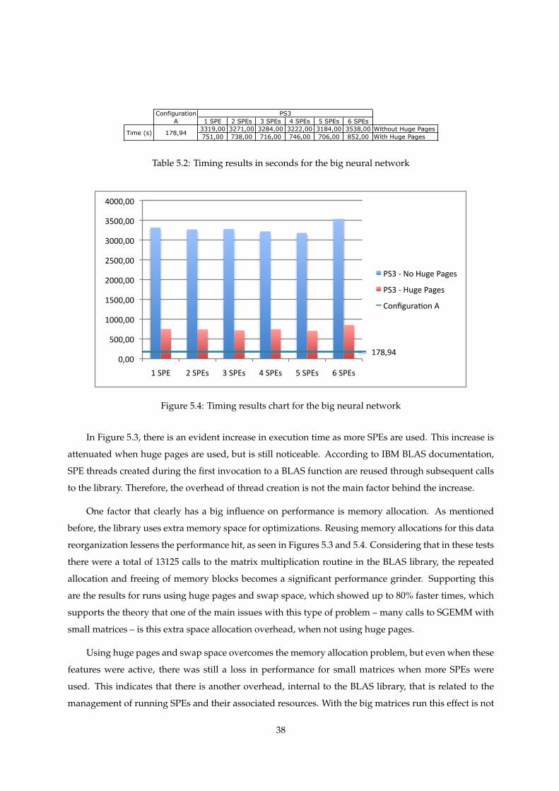
1 SPE 2 SPEs 3 SPEs 4 SPEs 5 SPEs 6 SPEs

3319,00 3271,00 3284,00 3222,00 3184,00 3538,00 Without Huge Pages

751,00 738,00 716,00 746,00 706,00 852,00 With Huge Pages178,94

Configuration

A

PS3

Time (s)

Table 5.2: Timing results in seconds for the big neural network

178,94 0,00 

500,00 

1000,00 

1500,00 

2000,00 

2500,00 

3000,00 

3500,00 

4000,00 

1 SPE  2 SPEs  3 SPEs  4 SPEs  5 SPEs  6 SPEs 

PS3 ‐ No Huge Pages 

PS3 ‐ Huge Pages 

Configura=on A 

Figure 5.4: Timing results chart for the big neural network

In Figure 5.3, there is an evident increase in execution time as more SPEs are used. This increase is

attenuated when huge pages are used, but is still noticeable. According to IBM BLAS documentation,

SPE threads created during the first invocation to a BLAS function are reused through subsequent calls

to the library. Therefore, the overhead of thread creation is not the main factor behind the increase.

One factor that clearly has a big influence on performance is memory allocation. As mentioned

before, the library uses extra memory space for optimizations. Reusing memory allocations for this data

reorganization lessens the performance hit, as seen in Figures 5.3 and 5.4. Considering that in these tests

there were a total of 13125 calls to the matrix multiplication routine in the BLAS library, the repeated

allocation and freeing of memory blocks becomes a significant performance grinder. Supporting this

are the results for runs using huge pages and swap space, which showed up to 80% faster times, which

supports the theory that one of the main issues with this type of problem – many calls to SGEMM with

small matrices – is this extra space allocation overhead, when not using huge pages.

Using huge pages and swap space overcomes the memory allocation problem, but even when these

features were active, there was still a loss in performance for small matrices when more SPEs were

used. This indicates that there is another overhead, internal to the BLAS library, that is related to the

management of running SPEs and their associated resources. With the big matrices run this effect is not

38

as noticeable, but still present.

This case illustrates how the Cell may not be a friendly platform for newcomers. A programmer

simply porting an application to this new platform in search of easy acceleration of his code by using

one of the level 3, Cell-optimized, BLAS functions, may find that some reengineering of the original

implementation and experimentation with the available tools (e.g. huge pages) is needed to obtain

performance gains.

5.4 Matrix Multiplication Server

Tests for this application were done on all three platforms. However, since both the PS3 and the GPU

have strong memory limitations, the maximum matrix dimensions tested on these machines were lower.

In the case of the PS3, only matrices of up to 4096x4096 were considered for the results presented as the

next larger size (4224x4224) caused memory swapping and therefore much worse results. The results

for configuration B do not show values over 6272x6272 since larger matrices hit the memory limit for

the device and originated program errors.

The average execution time for each matrix size and number of SPEs used, displayed in Figure 5.5,

especially the clear increase in performance for 6 SPEs and 4096x4096 matrices, provide interesting in-

dicators. With the increase of computational power from 1 to 6 SPEs, the time needed to calculate the

product of two 4096x4096 matrices was reduced by more than 70%, which suggests that an overhead

exists that reduces the performance-wise scalability. This overhead lies in the DMA transfer time to

SPE execution time ratio, with the SPEs occasionally stalling while input data is transferred to the LS or

results are sent DMA-ed to main memory. These results support the idea that the Cell needs a very high

arithmetic intensity (Harris, 2005) to provide good performance.

To make a comparison, we have presented timing and performance graphs in Figures 5.6

through 5.8. There are several aspects worthy of note.

First, although Configuration A’s performance is the worst out of the three tested for large sizes, it

was the one with the smallest variation in computing speed. This was because performance, in this case,

hit the CPU wall. Configuration B showed poor results for small matrix sizes, caused by the overhead

of thread and block initializations, but for larger sizes the GeForce’s speed trumped these fixed costs.

The execution times indicate that the GPU operates on a much smaller problem space, memory-wise.

The PS3 was the most limited platform of the three in regard to the amount of available mem-

ory. However, within these limits it showed results close to the theoretical peak speed for the Cell (25

GFLOPS per SPE). The QS20 showed higher speeds, proportional to the number of SPEs used.

39

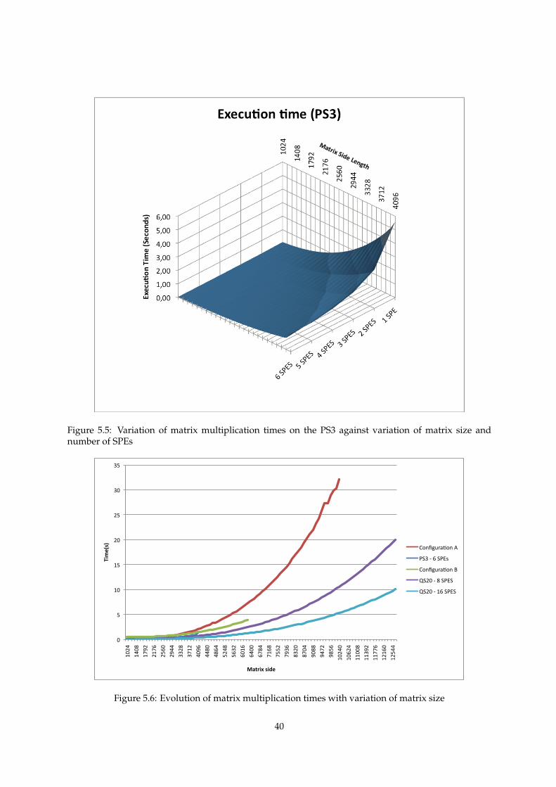
Figure 5.5: Variation of matrix multiplication times on the PS3 against variation of matrix size andnumber of SPEs

0 

5 

10 

15 

20 

25 

30 

35 

1024

 

1408

 

1792

 

2176

 

2560

 

2944

 

3328

 

3712

 

4096

 

4480

 

4864

 

5248

 

5632

 

6016

 

6400

 

6784

 

7168

 

7552

 

7936

 

8320

 

8704

 

9088

 

9472

 

9856

 

1024

0 

1062

4 

1100

8 

1139

2 

1177

6 

1216

0 

1254

4 

Time(s) 

Matrix side 

Configura4on A 

PS3 ‐ 6 SPEs 

Configura4on B 

QS20 ‐ 8 SPES 

QS20 ‐ 16 SPES 

Figure 5.6: Evolution of matrix multiplication times with variation of matrix size

40

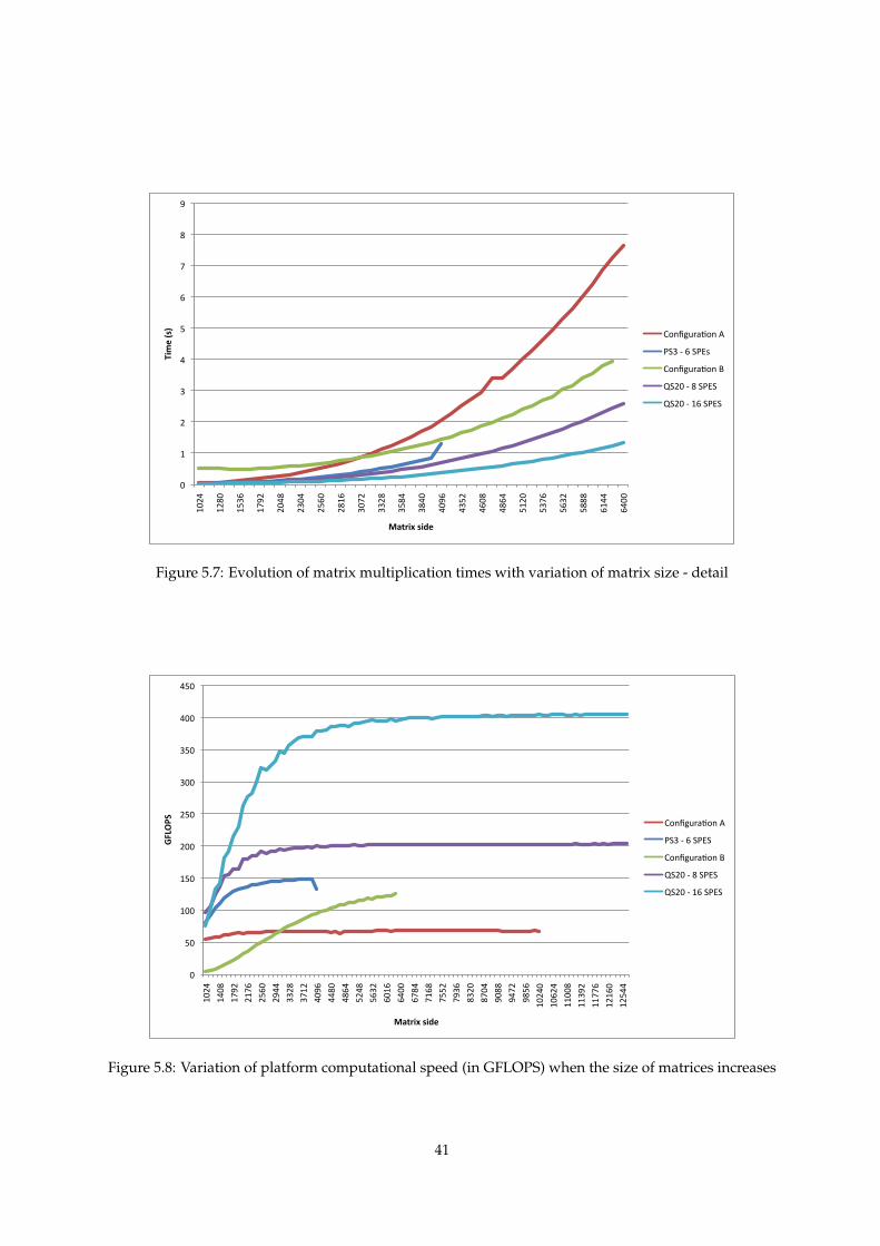
0 

1 

2 

3 

4 

5 

6 

7 

8 

9 10

24 

1280

 

1536

 

1792

 

2048

 

2304

 

2560

 

2816

 

3072

 

3328

 

3584

 

3840

 

4096

 

4352

 

4608

 

4864

 

5120

 

5376

 

5632

 

5888

 

6144

 

6400

 

Time (s) 

Matrix side 

Configura4on A 

PS3 ‐ 6 SPEs 

Configura4on B 

QS20 ‐ 8 SPES 

QS20 ‐ 16 SPES 

Figure 5.7: Evolution of matrix multiplication times with variation of matrix size - detail

0 

50 

100 

150 

200 

250 

300 

350 

400 

450 

1024

 

1408

 

1792

 

2176

 

2560

 

2944

 

3328

 

3712

 

4096

 

4480

 

4864

 

5248

 

5632

 

6016

 

6400

 

6784

 

7168

 

7552

 

7936

 

8320

 

8704

 

9088

 

9472

 

9856

 

1024

0 

1062

4 

1100

8 

1139

2 

1177

6 

1216

0 

1254

4 

GFLOPS 

Matrix side 

Configura4on A 

PS3 ‐ 6 SPES 

Configura4on B 

QS20 ‐ 8 SPES 

QS20 ‐ 16 SPES 

Figure 5.8: Variation of platform computational speed (in GFLOPS) when the size of matrices increases

41

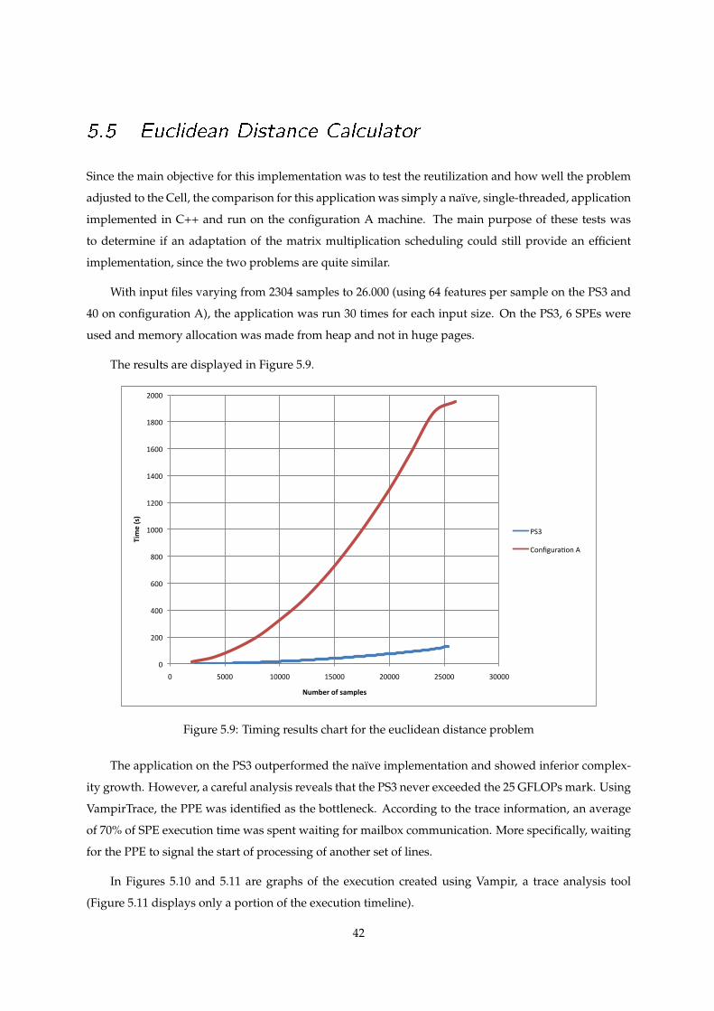
5.5 Euclidean Distance Calculator

Since the main objective for this implementation was to test the reutilization and how well the problem

adjusted to the Cell, the comparison for this application was simply a naıve, single-threaded, application

implemented in C++ and run on the configuration A machine. The main purpose of these tests was

to determine if an adaptation of the matrix multiplication scheduling could still provide an efficient

implementation, since the two problems are quite similar.

With input files varying from 2304 samples to 26.000 (using 64 features per sample on the PS3 and

40 on configuration A), the application was run 30 times for each input size. On the PS3, 6 SPEs were

used and memory allocation was made from heap and not in huge pages.

The results are displayed in Figure 5.9.

0 

200 

400 

600 

800 

1000 

1200 

1400 

1600 

1800 

2000 

0  5000  10000  15000  20000  25000  30000 

Time (s) 

Number of samples 

PS3 

Configura4on A 

Figure 5.9: Timing results chart for the euclidean distance problem

The application on the PS3 outperformed the naıve implementation and showed inferior complex-

ity growth. However, a careful analysis reveals that the PS3 never exceeded the 25 GFLOPs mark. Using

VampirTrace, the PPE was identified as the bottleneck. According to the trace information, an average

of 70% of SPE execution time was spent waiting for mailbox communication. More specifically, waiting

for the PPE to signal the start of processing of another set of lines.

In Figures 5.10 and 5.11 are graphs of the execution created using Vampir, a trace analysis tool

(Figure 5.11 displays only a portion of the execution timeline).

42

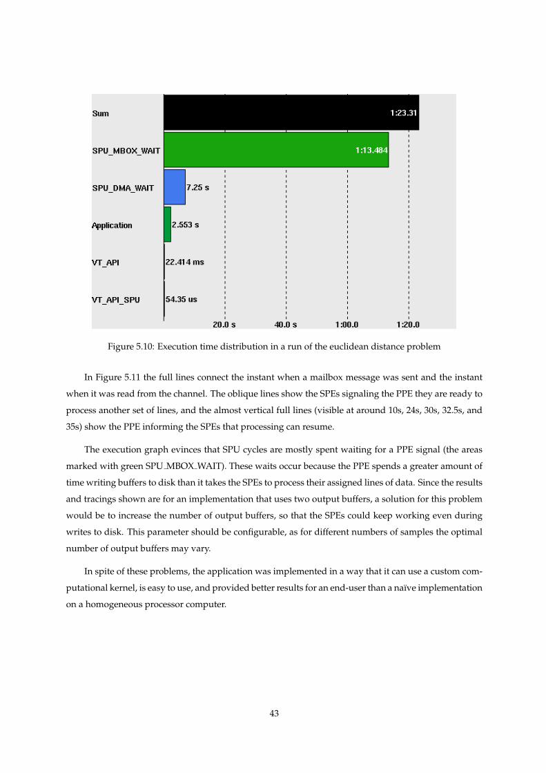
Figure 5.10: Execution time distribution in a run of the euclidean distance problem

In Figure 5.11 the full lines connect the instant when a mailbox message was sent and the instant

when it was read from the channel. The oblique lines show the SPEs signaling the PPE they are ready to

process another set of lines, and the almost vertical full lines (visible at around 10s, 24s, 30s, 32.5s, and

35s) show the PPE informing the SPEs that processing can resume.

The execution graph evinces that SPU cycles are mostly spent waiting for a PPE signal (the areas

marked with green SPU MBOX WAIT). These waits occur because the PPE spends a greater amount of

time writing buffers to disk than it takes the SPEs to process their assigned lines of data. Since the results

and tracings shown are for an implementation that uses two output buffers, a solution for this problem

would be to increase the number of output buffers, so that the SPEs could keep working even during

writes to disk. This parameter should be configurable, as for different numbers of samples the optimal

number of output buffers may vary.

In spite of these problems, the application was implemented in a way that it can use a custom com-

putational kernel, is easy to use, and provided better results for an end-user than a naıve implementation

on a homogeneous processor computer.

43

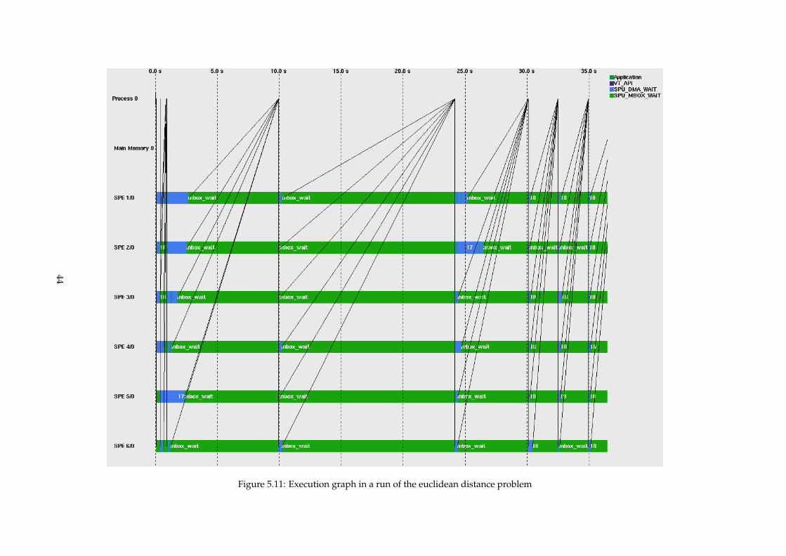
Figure 5.11: Execution graph in a run of the euclidean distance problem

44

5.6 Summary

The applications in this chapter provided results that shed a light on the applicability of the Cell in

matrix processing and related areas. The neural networks case represented the naıve approach to the

Cell, where no SPE or optimized code was written by the programmer, and only the porting to the

Cell-optimized BLAS library was done.

This case study supports the knowledge of the Cell’s need for arithmetic intensity. The existence of

the SPE setup overhead (thread and memory allocation, DMA transfers for input) can be minimized via

optimization techniques like the reuse of resources done by the BLAS library across invocations and can

be made less significant when there are large volumes of data to process.

The matrix multiplication case made clear that the theoretical peak performance is reachable in

practice, and showed how this platform, when approaching very delimited problems where there is

room for optimizations, can outperform other players in the field of high performance computing.

Finally, the euclidean distance revisited the programming effort perspective, stressing that the im-

plementation process on the Cell requires that a significant amount of time be put into designing the

algorithm while taking into account the Cell’s idiosyncrasies and limitations.

45

46

6Conclusions

6.1 Conclusions

The neural networks case represented the naive approach to the Cell, where no SPE or optimized code

was written by the programmer, and only the porting to the Cell-optimized BLAS library was done. The

results showed that it is neither trivial nor immediate to increase an application’s performance simply

by moving it to a Cell processor. In this particular case, there were not enough calculations done on the

SPEs to mask the overheads of memory allocation and processor management. The SPE setup overhead

can also be mitigated via optimization techniques like the reuse of resources done by the BLAS library

across invocations and can be made less significant when there are large volumes of data to process.

Analysis on the matrix multiplication case study reveals this to be a problem well adjusted for the

Cell’s capabilities. It has a simple scheduling scheme and a good balance between the amount of data

transmitted between PPE and SPE and the calculations done on those chunks of data. However, the code

used to attain the performance gains presented was quite complex, especially the computational kernel,

and for large matrices there may be cases where using cuBLAS on a GPU may be a good compromise

between high performance and programming effort.

The current version of our BLAS server performs no type of load balancing or job queueing, but in

the future this application could become a simple interface for users on other platforms (like Configura-

tion A used for testing) to perform fast matrix multiplication. In this perspective, of the user and not the

programmer, the PS3 would provide the performance gain at little expense in terms of programming

complexity. This scenario, however, is only true in the case that network speed is high enough so that

the transmission time does not outweigh the decrease in processing time.

The euclidean distance case showed how the Cell’s complexity and limitations can hinder even

an optimized program. Although care was taken to overlap DMA transfers with computation and to

program a SIMD-ized kernel, performance was lower than expected due to the low memory capacity of

the PS3 and the amount of control code left on the PPE.

Reutilization of the scheduling from one Cell program to another is a possible solution to lessen

the programmer’s work complexity. However, a new problem may require data dependencies that

require an entirely new scheduling algorithm. On the other hand, application programmers whose data

is organized and processed in a similar manner to the euclidean distance problem, for example, could

use this application’s code and simply program a new computational kernel, as it was isolated from the

rest of the SPE code for flexibility.

One other factor of more and more relevance today is the energy consumption of computers. Ac-

cording to data from Green500 (see www.green500.org), the top 7 out of the 10 most energy-efficient

supercomputers in the world were Cell-based (November 2008). Included in these 7 is the Roadrunner

project, built in Los Alamos (Barker et al., 2008), which is currently ranked as the fastest supercomputer

in the world.

Concluding, the Cell is, as a platform, interesting to different types of stakeholders, each with their

concerns. To the end users of optimized applications, the Cell provides both the advantage of having

cluster software like MPI available and therefore being able to be integrated into the existing resources

as well as a significant performance increase. To developers, it requires a strong analysis of data orga-

nization and significant amount of effort put into learning the platform and designing the application.

Finally, for the financial investors, it provides good ratios in terms of GFLOPS per $ and GFLOPS per

Watt, helping contain the maintenance costs of a cluster or supercomputer.

6.2 Future Work

Following the guiding line of this work, solutions to other natural language problems should be imple-

mented to further explore and outline the Cell’s preferred domain. Like what has been presented here,

these implementations’ evaluation should also take into account the development effort and comparison

to other platforms.

Although there are clusters using Cell processors, the most publicized example being the Roadrun-

ner cluster (Barker et al., 2008), it would be interesting to investigate Cell performance when in a cluster,

to identify the impacts of a load scheduling and work partitioning algorithm.

The GPUs, which have been explored only very lightly in this work, should also be further inves-

tigated and compared against the Cell, as they are a quite common resource and may, in theory, have

better expected performance than the Cell.

Finally, the euclidean distance case study could, aided by performance analysis tools, be redesigned

and implemented along a different algorithm, to obtain better results.

48

Bibliography

Al Geist, W., Huss-Lederman, S., Lumsdaine, A., Lusk, E., Saphir, W., Skjellum, T., et al. (1996). MPI-2:

Extending the Message-Passing Interface. Euro-Par, 96.

Barker, K. J., Davis, K., Hoisie, A., Kerbyson, D. J., Lang, M., Pakin, S., et al. (2008). Entering the petaflop

era: the architecture and performance of roadrunner. In Sc ’08: Proceedings of the 2008 acm/ieee

conference on supercomputing (pp. 1–11). Piscataway, NJ, USA: IEEE Press.

Blackford, S., Corliss, G., Demmel, J., Dongarra, J., Duff, I., Hammarling, S., et al. (2001). Document for the

Basic Linear Algebra Subprograms (BLAS) standard: BLAS Technical Forum.

Bouzas, B., Cooper, R., Greene, J., Pepe, M., & Prelle, M. (2006). MultiCore Framework: An API for

Programming Heterogeneous Multicore Processors.

Buck, I., Foley, T., Horn, D., Sugerman, J., Fatahalian, K., Houston, M., et al. (2004). Brook for GPUs:

stream computing on graphics hardware. ACM Transactions on Graphics (TOG), 23(3), 777–786.

Dean, J., & Ghemawat, S. (2004). MapReduce: Simplified Data Processing on Large Clusters.

Eichenberger, A., O’Brien, J., O’Brien, K., Wu, P., Chen, T., Oden, P., et al. (2006). Using advanced compiler

technology to exploit the performance of the Cell Broadband EngineTM architecture-Author Bios.

IBM Systems Journal, 45(1).

Fatahalian, K., Horn, D., Knight, T., Leem, L., Houston, M., Park, J., et al. (2006). Sequoia: programming the

memory hierarchy.

Frey, B. (2005). PowerPC Architecture Book. (http://www.ibm.com/developerworks/eserver/

library/es-archguide-v2.html (Visited on 2008/01/29))

Hackenberg, D. (2008). Fast Matrix Multiplication on Cell (SMP) Systems. (http://www.tu-dresden.

de/zih/cell/matmul (Visited on 2008/03/01))

Harris, M. (2005). Mapping computational concepts to GPUs. In Siggraph ’05: Acm siggraph 2005 courses

(p. 50-52). New York, NY, USA: ACM.

Hofstee, H. P. (2005, May). Introduction to the Cell Broadband Engine (Tech. Rep.). IBM.

IBM. (2007a). Accelerated Library Framework for Cell Broadband Engine Programmer’s Guide and API Reference.

49

IBM. (2007b). Basic Linear Algebra Subprograms Programmer’s Guide and API Reference.

IBM. (2007c, April). Cell Broadband Engine Programming Handbook. IBM.

IBM. (2007d). Data Communication and Synchronization Library for Cell Broadband Engine Programmer’s Guide

and API Reference.

IBM. (2007e). IBM Full-System Simulator User’s Guide.

IBM. (2007f). Using the single-source compiler, IBM XL C/C++ Alpha Edition for Multicore Acceleration for

Linux,V0.9.

IBM. (2008a). IBM Cell BladeCenter. (http://www-03.ibm.com/systems/bladecenter/hardware/

servers/cell.html (Visited on 2008/01/25))

IBM. (2008b). IBM Power Architecture: A High-Performance Architecture with a History. (http:

//www-03.ibm.com/systems/p/hardware/whitepapers/power/ppc_arch.html?S_

TACT=105AGX16&S_CMP=ART (Visited on 15/07/2008))

Jain, A. K., Mao, J., & Mohiuddin, K. M. (1996). Artificial neural networks: A tutorial. IEEE Computer,

29(3), 31-44.

Kahle, J., Day, M., Hofstee, H., Johns, C., Maeurer, T., & Shippy, D. (2005). Introduction to the Cell

multiprocessor. IBM JOURNAL OF RESEARCH AND DEVELOPMENT, 49(4/5), 589.

Kistler, M., Perrone, M., & Petrini, F. (2006). Cell multiprocessor communication network: Built for speed.

IEEE Micro, 26(3), 10–23.

Kruijf, M. de, & Sankaralingam, K. (2007). MapReduce for the Cell BE Architecture (Tech. Rep.). University

of Wisconsin.

Logan, B. (2000). Mel frequency cepstral coefficients for music modeling.

Makhoul, J. (1975, April). Linear prediction: A tutorial review. Proceedings of the IEEE, 63(4), 561-580.

May, C., Silha, E., Simpson, R., & Warren, H. (1994). The PowerPC architecture: a specification for a new family

of RISC processors. Morgan Kaufmann Publishers Inc. San Francisco, CA, USA.

Monteyne, M. (2007). RapidMind Multi-Core Development Platform White Paper (Confidential) (Tech. Rep.).

Rapidmind Inc.

MPI. (2008, January). The Message Passing Interface standard. (http://www-unix.mcs.anl.gov/mpi/

(Visited on 2008/01/11))

Mueller, C. (2007). Synthetic Programming: User-Directed Run-Time Code Synthesis For High Performance

Computing. Unpublished doctoral dissertation, Indiana University.

50

NVIDIA. (2008, July). Cuda programming guide version 2.0.

NVIDIA. (2009). SLI Zone. (http://www.slizone.com (Visited on 2008/01/25))

OpenMP. (2008). The OpenMP specification for parallel programming. (http://www.openmp.org/ (Visited

on 2008/01/07))

Python. (2008). Python Language Home. (http://www.python.org (Visited on 2008/01/26))

Rambus. (2008). Rambus xdr. (http://www.rambus.com/us/products/xdr/index.html (Visited

on 18/07/2008))

RapidMind. (2008). RapidMind Product Overview. (http://www.rapidmind.net/product.php (Vis-

ited on 2008/01/27))

Santos Meinedo, H. dos. (2008). Audio Pre-processing and Speech Recognition for Broadcast News. Unpub-

lished doctoral dissertation, Universidade Tecnica de Lisboa.

Sony. (2008). Playstation 3 Home. (http://www.us.playstation.com/PS3 (Visited on 2008/01/25))

Tabak, D. (1986). Reduced instruction set computer–risc–architecture. New York, NY, USA: John Wiley &

Sons, Inc.

51

52

IAppendices

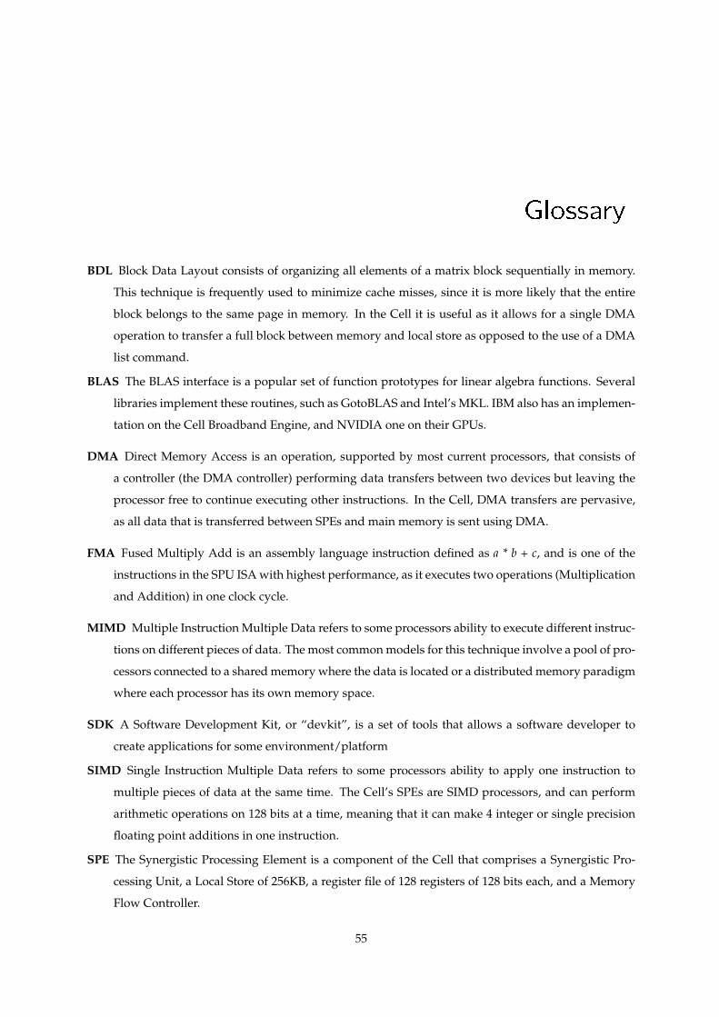
Glossary

BDL Block Data Layout consists of organizing all elements of a matrix block sequentially in memory.

This technique is frequently used to minimize cache misses, since it is more likely that the entire

block belongs to the same page in memory. In the Cell it is useful as it allows for a single DMA

operation to transfer a full block between memory and local store as opposed to the use of a DMA

list command.

BLAS The BLAS interface is a popular set of function prototypes for linear algebra functions. Several

libraries implement these routines, such as GotoBLAS and Intel’s MKL. IBM also has an implemen-

tation on the Cell Broadband Engine, and NVIDIA one on their GPUs.

DMA Direct Memory Access is an operation, supported by most current processors, that consists of

a controller (the DMA controller) performing data transfers between two devices but leaving the

processor free to continue executing other instructions. In the Cell, DMA transfers are pervasive,

as all data that is transferred between SPEs and main memory is sent using DMA.

FMA Fused Multiply Add is an assembly language instruction defined as a * b + c, and is one of the

instructions in the SPU ISA with highest performance, as it executes two operations (Multiplication

and Addition) in one clock cycle.

MIMD Multiple Instruction Multiple Data refers to some processors ability to execute different instruc-

tions on different pieces of data. The most common models for this technique involve a pool of pro-

cessors connected to a shared memory where the data is located or a distributed memory paradigm

where each processor has its own memory space.

SDK A Software Development Kit, or “devkit”, is a set of tools that allows a software developer to

create applications for some environment/platform

SIMD Single Instruction Multiple Data refers to some processors ability to apply one instruction to

multiple pieces of data at the same time. The Cell’s SPEs are SIMD processors, and can perform

arithmetic operations on 128 bits at a time, meaning that it can make 4 integer or single precision

floating point additions in one instruction.

SPE The Synergistic Processing Element is a component of the Cell that comprises a Synergistic Pro-

cessing Unit, a Local Store of 256KB, a register file of 128 registers of 128 bits each, and a Memory

Flow Controller.

55

56

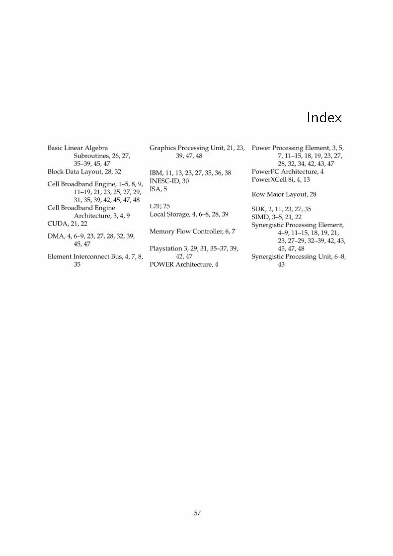
Index

Basic Linear AlgebraSubroutines, 26, 27,35–39, 45, 47

Block Data Layout, 28, 32

Cell Broadband Engine, 1–5, 8, 9,11–19, 21, 23, 25, 27, 29,31, 35, 39, 42, 45, 47, 48

Cell Broadband EngineArchitecture, 3, 4, 9

CUDA, 21, 22

DMA, 4, 6–9, 23, 27, 28, 32, 39,45, 47

Element Interconnect Bus, 4, 7, 8,35

Graphics Processing Unit, 21, 23,39, 47, 48

IBM, 11, 13, 23, 27, 35, 36, 38INESC-ID, 30ISA, 5

L2F, 25Local Storage, 4, 6–8, 28, 39

Memory Flow Controller, 6, 7

Playstation 3, 29, 31, 35–37, 39,42, 47

POWER Architecture, 4

Power Processing Element, 3, 5,7, 11–15, 18, 19, 23, 27,28, 32, 34, 42, 43, 47

PowerPC Architecture, 4PowerXCell 8i, 4, 13

Row Major Layout, 28

SDK, 2, 11, 23, 27, 35SIMD, 3–5, 21, 22Synergistic Processing Element,

4–9, 11–15, 18, 19, 21,23, 27–29, 32–39, 42, 43,45, 47, 48

Synergistic Processing Unit, 6–8,43

57

58