International Spillovers of Large-Scale Asset Purchases∗

Sami Alpanda†

Bank of Canada

Serdar Kabaca‡

Bank of Canada

August 2014

FIRST DRAFT

Abstract

This paper evaluates the international spillover effects of large-scale asset purchases (LSAPs) using a

two-country dynamic stochastic general equilibrium model with nominal and real rigidities and portfolio

balance effects. Portfolio balance effects arise from imperfect substitution between short and long-term

bonds in both domestic and foreign portfolios of each country. We show that LSAPs can stimulate

domestic and foreign activity and lower both domestic and foreign long-term yields. The international

spillover effects increase when foreigners hold more long-term bonds in their foreign-asset portfolios at the

steady state or their elasticity of substitution between short-term and long-term bonds is smaller. We find

larger spillover effects of U.S. asset purchases than U.S. conventional monetary policy because foreigners’

U.S. bond holdings are heavily weighted towards long-term bonds.

Keywords: Portfolio balance effects, international spillovers, preferred habitat, DSGE.

JEL Classification:

∗We thank Rhys Mendes, Subrata Sarker, Yuko Imora, Abeer Reza, and seminar participants at the Bank of Canada forsuggestions and comments. All remaining errors are our own. The views expressed in this paper are those of the authors. Noresponsibility should be attributed to the Bank of Canada.†Bank of Canada, Canadian Economic Analysis Department, 234 Wellington Street, Ottawa, Ontario K1A 0G9, Canada.

Phone: (613) 782-7619, e-mail: alpa@bankofcanada.ca.‡Bank of Canada, International Economic Analysis Department, 234 Wellington Street, Ottawa, Ontario K1A 0G9, Canada.

Phone: (613) 782-7509, e-mail: kaba@bankofcanada.ca.

1

1 Introduction

Following the financial turbulence in the fall of 2008, the Federal Reserve cut short-term policy rates to

near-zero and announced unprecedented unconventional policy measures, such as large-scale asset purchases

(LSAPs; also known as quantitative easing, “QE”), at the zero lower bound. Several studies have found signif-

icant effects from these asset purchases in terms of lowering U.S. long-term yields and strengthening economic

activity (see Baumeister and Benati, 2013, D’amico et. al, 2012, and Krishnamurthy and Vissing-Jorgensen,

2011 among others). The domestic effects of these policies may have also increased the attractiveness of

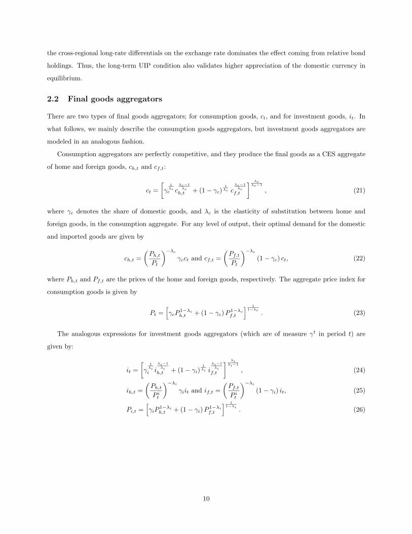
foreign assets, and led to portfolio re-balancing by investors. Figure 1 shows exchange rate and long-term

yield movements in countries where the policy rates were not significantly binding and QE-like unconventional

measures were not expected. The figure suggests that the currencies of these countries tended to appreciate

during and after the announcement of LSAPs in the U.S.1 Long-term yields were also in declining trend

during this period; on average long-term rates fell by more than 1% by mid-2013 when tapering talk started.2

In their analyses, Bauer and Neely (2014), and Neely (2013) find substantial effects of LSAPs on interna-

tional financial markets by lowering foreign yields and depreciating the U.S. dollar in a sample of advanced

economies. Chen et al. (2011) and Fratzscher et al. (2012) also document significant spillovers of QE into

financial markets in emerging economies.

In this paper, we propose a two-country, open-economy model in which foreigners hold both short-term

and long-term U.S. government bonds, as well as their domestic bonds, but do not fully substitute among

these bonds based on portfolio preferences. We show that the model can generate the type of international

spillovers mentioned above after a QE announcement in the U.S. through the portfolio balance channel. We

capture these portfolio balance effects by introducing a portfolio preference in households’ utility function

with a CES structure to aggregate individual financial assets. The imperfect substitution between short-

term and long-term assets, as well as between domestic and foreign assets could represent attitutes towards

differential risk on these assets, cost of portfolio adjustment, and the institutional use of these bonds for

liquidity purposes with varying degrees.3 Since long-term and short-term bonds are not perfect substitutes

in our set-up, long-term rates fall as a response to a drop in their relative supply even when short-term rates

remain constant.4 Lower long-term rates then stimulate the domestic economy and generate appreciation

pressures on the currency of the rest of the world (ROW) economy. This in turn leads to current and

expected policy rates to fall in the ROW, lowering foreign long-term yields as well. Finally, lower short-term

1IMF data also indicate that the central banks of emerging market economies (EMEs) increased their U.S. dollar-denominatedreserves during these episodes, partly to offset these appreciation pressures on their currencies.

2Long-term yields increased in the beginning of LSAP2 mainly because central banks in many countries hiked interest rates inexpectation of higher inflation. However, this tightening cycle was short (about a year) as these expectations did not materialize.Contagious effects from the Euro crisis could have also put upward pressure on the yields during this period.

3Financial institutions, for example, use short-term money market instruments in the interbank market. Thus, they may beless willing to alter their portfolio balances when there is a change in the relative prices of short-term to long-term assets.

4When long-term and short-term bonds are perfectly substitutable, exogenous changes in the relative supply of one type ofasset would have no effect on the relative price of bonds (see Curdia and Woodford, 2010).

2

Note: EMEs include Brazil, Chile, China, Colombia, Hungary, India, Indonesia, Israel, Korea, Malaysia, Mexico, Peru, Philippines,

Poland, Russia, South Africa, Taiwan, Thailand, Turkey. Small advanced economies include Australia, Canada, Denmark, Norway,

Sweden, Switzerland. Select Euro members are Austria, Finland, France, Germany, Netherlands.

Figure 1: Exchange Rates and Government Yields over 2010-2014

and long-term interest rates stimulate the economic activity in the ROW.

Another advantage of introducing maturity structure in an open economy model is that it allows us to

analyze the effects of maturity composition of U.S. government bonds in foreigners’ portfolio. The motivation

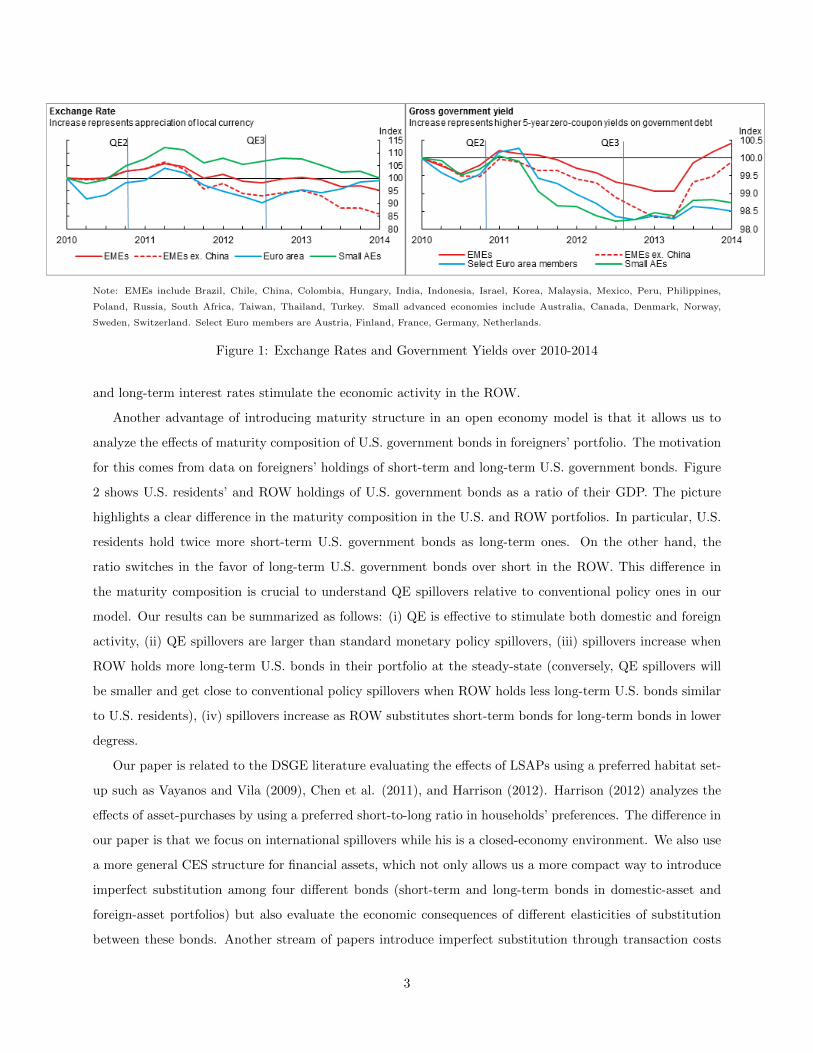
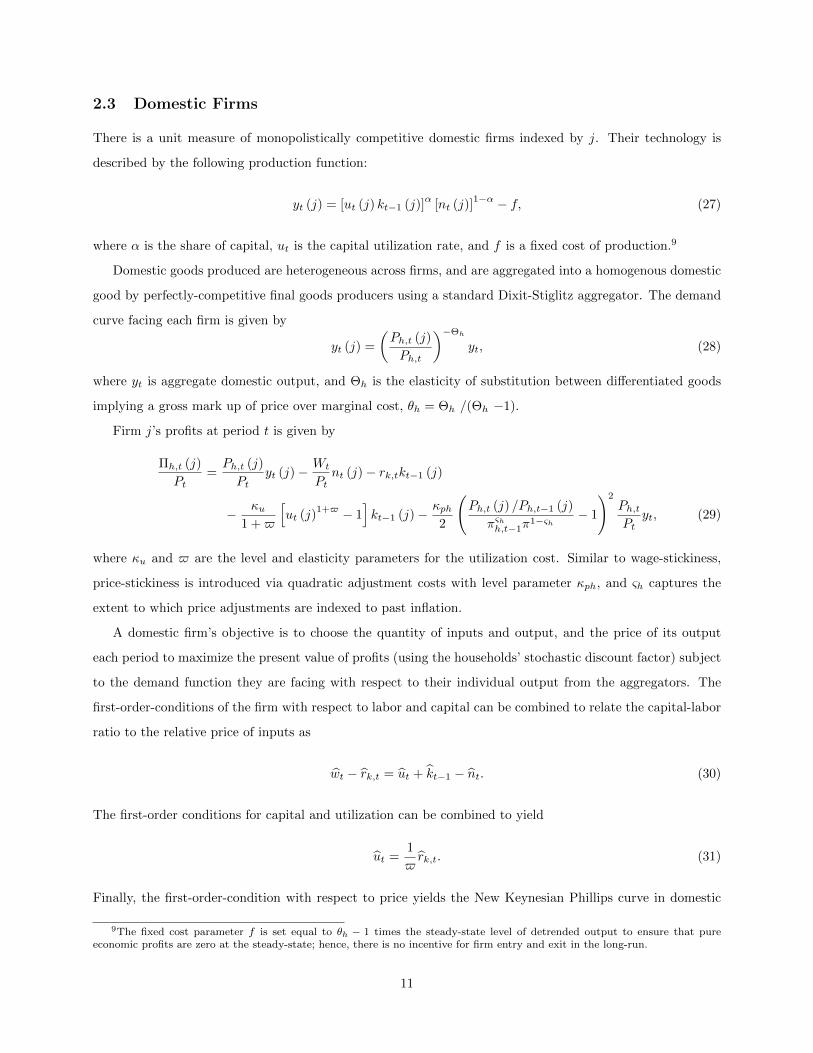
for this comes from data on foreigners’ holdings of short-term and long-term U.S. government bonds. Figure

2 shows U.S. residents’ and ROW holdings of U.S. government bonds as a ratio of their GDP. The picture

highlights a clear difference in the maturity composition in the U.S. and ROW portfolios. In particular, U.S.

residents hold twice more short-term U.S. government bonds as long-term ones. On the other hand, the

ratio switches in the favor of long-term U.S. government bonds over short in the ROW. This difference in

the maturity composition is crucial to understand QE spillovers relative to conventional policy ones in our

model. Our results can be summarized as follows: (i) QE is effective to stimulate both domestic and foreign

activity, (ii) QE spillovers are larger than standard monetary policy spillovers, (iii) spillovers increase when

ROW holds more long-term U.S. bonds in their portfolio at the steady-state (conversely, QE spillovers will

be smaller and get close to conventional policy spillovers when ROW holds less long-term U.S. bonds similar

to U.S. residents), (iv) spillovers increase as ROW substitutes short-term bonds for long-term bonds in lower

degress.

Our paper is related to the DSGE literature evaluating the effects of LSAPs using a preferred habitat set-

up such as Vayanos and Vila (2009), Chen et al. (2011), and Harrison (2012). Harrison (2012) analyzes the

effects of asset-purchases by using a preferred short-to-long ratio in households’ preferences. The difference in

our paper is that we focus on international spillovers while his is a closed-economy environment. We also use

a more general CES structure for financial assets, which not only allows us a more compact way to introduce

imperfect substitution among four different bonds (short-term and long-term bonds in domestic-asset and

foreign-asset portfolios) but also evaluate the economic consequences of different elasticities of substitution

between these bonds. Another stream of papers introduce imperfect substitution through transaction costs

3

Note: Short term bonds include US treasury securities with a maturity of less than one year, financial institutions’ reserves at the Federal

Reserve System, vault cash and currency outside banks. Long-term bonds consist of US Treasury bills with a maturity of more than one

year

Figure 2: US Residents’ and ROW Holdings of US Short-term and Long-term Government Bonds

on the long-term bond in a New-Keynesian model such as Chen et al.(2011). Dorich et al. (2012) study small

open economy consequences of this type of set-up but do not study the spillover effects of QE policies to the

rest of the world. Note that these models require restricted agents that hold only long-term bonds to generate

a real effect on aggregate demand from changes in long-term rates while short-term rates stay constant. In our

set-up, though, we do not need to introduce these types of agents because when household gets utility from

holding financial assets, their marginal decisions between holding a short-term bond and spending depend

not only on short-term rates but also on the quantity of short-term bonds holdings. Large increases in the

U.S. short-term bond holdings following QE lowers the marginal benefit of holding these bonds, thus making

it less attractive relative to consuming even when the domestic short-term rates remain constant.

The remainder of the paper proceeds as follows. The next section introduces the model. Section 3

discusses the calibration of the model. Section 4 presents the results of the QE experiment. Section 5

conducts sensitivity analyses, and section 6 concludes.

2 Model

The model is a two-country large-open-economy DSGE model with real and nominal rigidities, and portfolio

balance effects.5 The latter is achieved through modeling households’ preferences on the composition of

their financial portfolio, which generates imperfect substitution between short and long-term assets for both

5We assume that both regions have the same economic size motivated by the fact that output from the countries that facedzero lower bound in the end of 2010 - the U.S., the U.K. and Japan - constitute more than %46 of the world GDP over thesample period 1960-2010. The ratio is similar when we take a more recent period 2000-2010.

4

domestic and foreign soverign debt, and therefore enables QE to have real effects on the economy.

Each country in the model is populated by households, capital producers, final goods aggregators, domestic

producers, and importers, as well as fiscal and monetary policy rules. In what follows, we focus on the agents

in the domestic economy, but the foreign economy is analogous in our set-up. When variables from the foreign

economy are necessary, we denote them with a (*) superscript.

2.1 Households

The economy is populated by a unit measure of infinitely-lived patient households indexed by i, whose

intertemporal preferences over consumption, ct, financial asset portfolio, at, and labor supply, nt, are described

by the following expected utility function:

Et

∞∑τ=t

βτ−t

[log [cτ (i) − ζcτ−1] + ξaaτ (i) − ξn

nτ (i)1+ϑ

1 + ϑ

], (1)

where t indexes time, β < 1 is the time-discount parameter, ζ is the external habit parameter for consumption,

ϑ is the inverse of the Frisch-elasticity of labor supply, and ξa and ξn are level parameters that determine the

relative importance of financial assets and labor in the utility function.

2.1.1 Preferences on portfolio composition

We capture imperfect substitution across assets of different currencies and maturities by using a nested CES

structure for financial assets. In particular, the asset portfolio in the utility function, at, is a CES aggregate

of the domestic portfolio, aH,t, and the foreign portfolio, aF,t:

at (i) =

[γ

1λaa [aH,t (i)]

λa−1λa + (1 − γa)

1λa [aF,t (i)]

λa−1λa

] λaλa−1

, (2)

where γa determines the share of home assets in the aggregate portfolio, and λa is the elasticity of substitution

between domestic and foreign assets.

The home-asset sub-portfolio is a CES aggregate of short-term government bonds, BHS,t, and long-term

domestic government bonds, BHL,t:

aH,t (i) =

γ 1λH

H

(BHS,t (i)

Pt

)λH−1

λH

+ (1 − γH)1λH

(qL,tBHL,t (i)

Pt

)λH−1

λH

λHλH−1

, (3)

where Pt is the aggregate price level, qL,t is the relative price of a domestic long-term bond, γH is the share

of short-term bonds in the home-asset portfolio, and λH is the elasticity of substitution between short and

long-term domestic bonds.

Similarly, the foreign-asset sub-portfolio is a CES aggregate of short-term foreign government bonds,

5

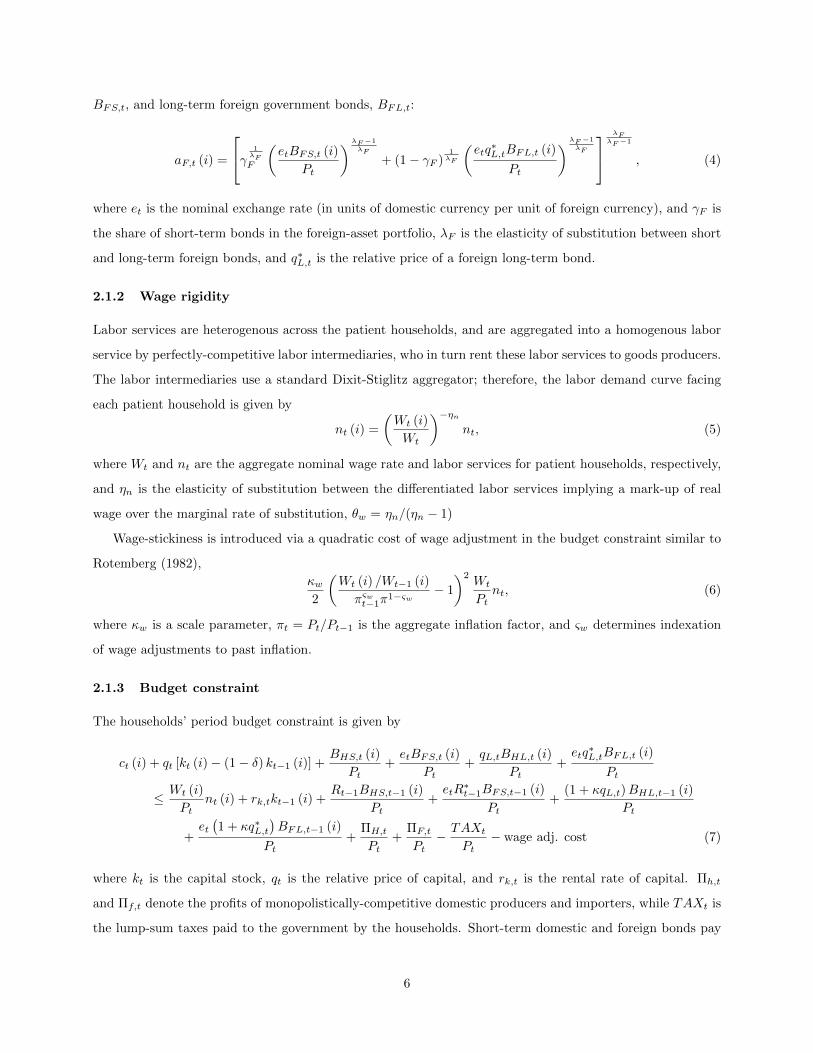
BFS,t, and long-term foreign government bonds, BFL,t:

aF,t (i) =

γ 1λF

F

(etBFS,t (i)

Pt

)λF−1

λF

+ (1 − γF )1λF

(etq∗L,tBFL,t (i)

Pt

)λF−1

λF

λFλF−1

, (4)

where et is the nominal exchange rate (in units of domestic currency per unit of foreign currency), and γF is

the share of short-term bonds in the foreign-asset portfolio, λF is the elasticity of substitution between short

and long-term foreign bonds, and q∗L,t is the relative price of a foreign long-term bond.

2.1.2 Wage rigidity

Labor services are heterogenous across the patient households, and are aggregated into a homogenous labor

service by perfectly-competitive labor intermediaries, who in turn rent these labor services to goods producers.

The labor intermediaries use a standard Dixit-Stiglitz aggregator; therefore, the labor demand curve facing

each patient household is given by

nt (i) =

(Wt (i)

Wt

)−ηnnt, (5)

where Wt and nt are the aggregate nominal wage rate and labor services for patient households, respectively,

and ηn is the elasticity of substitution between the differentiated labor services implying a mark-up of real

wage over the marginal rate of substitution, θw = ηn/(ηn − 1)

Wage-stickiness is introduced via a quadratic cost of wage adjustment in the budget constraint similar to

Rotemberg (1982),

κw2

(Wt (i) /Wt−1 (i)

πςwt−1π1−ςw

− 1

)2Wt

Ptnt, (6)

where κw is a scale parameter, πt = Pt/Pt−1 is the aggregate inflation factor, and ςw determines indexation

of wage adjustments to past inflation.

2.1.3 Budget constraint

The households’ period budget constraint is given by

ct (i) + qt [kt (i) − (1 − δ) kt−1 (i)] +BHS,t (i)

Pt+etBFS,t (i)

Pt+qL,tBHL,t (i)

Pt+etq∗L,tBFL,t (i)

Pt

≤ Wt (i)

Ptnt (i) + rk,tkt−1 (i) +

Rt−1BHS,t−1 (i)

Pt+etR∗t−1BFS,t−1 (i)

Pt+

(1 + κqL,t)BHL,t−1 (i)

Pt

+et(1 + κq∗L,t

)BFL,t−1 (i)

Pt+

ΠH,t

Pt+

ΠF,t

Pt− TAXt

Pt− wage adj. cost (7)

where kt is the capital stock, qt is the relative price of capital, and rk,t is the rental rate of capital. Πh,t

and Πf,t denote the profits of monopolistically-competitive domestic producers and importers, while TAXt is

the lump-sum taxes paid to the government by the households. Short-term domestic and foreign bonds pay

6

a pre-determined interest rate of Rt−1 and R∗t−1, while long-term bonds are perpetuities that pay a coupon

payment of 1 unit in the next period and coupon payments decaying at a rate of κ for each period after that

as in Woodford (2001). Since these long-term bonds are tradable, we can write them in recursive form in the

budget constraint above. The yields on domestic and foreign long-term bonds are defined respectively as

RL,t =1 + κqL,tqL,t

and R∗L,t =1 + κq∗L,tq∗L,t

. (8)

2.1.4 Optimality conditions

The households’ objective is to maximize utility subject to the budget constraint, the labor demand curve of

labor intermediaries, and appropriate No-Ponzi conditions. The first-order conditions for consumption and

capital are standard, and are given by

1

ct − ζct−1= λt, (9)

qt = Et

[(βλt+1

λt

)[(1 − δ) qt+1 + rk,t+1]

], (10)

where λt is the Lagrange multiplier on the budget constraint. Similarly, the optimality conditions with

respect to labor and wages can be combined to derive a New-Keynesian wage Phillips curve, which after

log-linearization can be written as:

πw,t − ςwπt−1 = βEt [πw,t+1 − ςwπt] −ηn − 1

κw

(wt − ϑnt −

1

1 − ζ(ct − ζct−1)

), (11)

where the nominal wage inflation, πw,t, and the real wage rate, wt, are related as

πw,t − πt = wt − wt−1. (12)

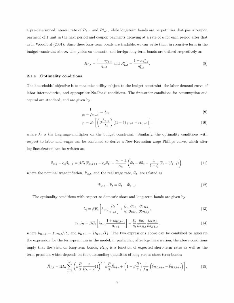
The optimality conditions with respect to domestic short and long-term bonds are given by

λt = βEt

[λt+1

Rtπt+1

]+ξaat

∂at∂aH,t

∂aH,t∂bHS,t

, (13)

qL,tλt = βEt

[λt+1

1 + κqL,t+1

πt+1

]+ξaat

∂at∂aH,t

∂aH,t∂bHL,t

, (14)

where bHS,t = BHS,t/Pt, and bHL,t = BHL,t/Pt. The two expressions above can be combined to generate

the expression for the term-premium in the model; in particular, after log-linearization, the above conditions

imply that the yield on long-term bonds, RL,t, is a function of expected short-term rates as well as the

term-premium which depends on the outstanding quantities of long versus short-term bonds:

RL,t = ΩEt

∞∑s=0

(βR

π

κ

RL − κΩ

)s [βR

πRt+s +

(1 − β

R

π

)1

λH

(bHL,t+s − bHS,t+s

)], (15)

7

with

Ω =1

1 −(1 − βRπ

) (1 − 1

λH

) . (16)

The equation above implies that, even when short rates are kept constant (e.g. at the zero-lower-bound),

the long-rate can be altered with asset purchase policies. Particularly, LSAP in the domestic economy

lowers the supply of long-term bonds and, in return, increases the supply of short-term bonds through the

consolidated budget constraint.6 When quantities involved are large, this can lower the yields on long-term

bonds, and affect aggregate demand even when short rates are constant. Note that, the portfolio preference

specification in our representative agent framework is crucial for this result, and is different than standard

models in the literature. For example, having lower rates by itself is not enough to stimulate the economy

even if (unrestricted) households hold both types of assets in Chen et al. (2012). This is because the marginal

utility of consumption depends on the short-term interest rate, which is constant at the zero lower bound.

However, in our model, the representative agent’s marginal utility depends not only on the short-term interest

rate but also on bond quantities. To see this, observe that the first-order-condition for short-term domestic

bonds (equation 13), yields the following expression after log-linearization (and setting portfolio elasticities

to 1):

λt = βR

π

(Etλt+1 + Rt − Etπt+1

)−(

1 − βR

π

)bHS,t. (17)

In the absence of the portfolio choice in preferences, βR/π would be equal to 1 at the steady-state, and the

equation above becomes the standard IS curve that makes aggregate demand to depend only on the real

interest rates. With our portfolio specification in preferences, the marginal benefit of holding short-term

bonds diminishes as short-term bond holdings increase; this stimulates aggregate demand even when short

rates are constant. Thus, our portfolio specification allows for changes in the outstanding quantity of bonds

to affect demand even in a representative agent framework, unlike papers in the literature which rely on

segmented markets (e.g. Chen et al., 2012, features restricted households which can only trade in long-term

assets).

Note that given the calibration in Section 3, the coefficient in from of the bond quantity term in equation

(17), 1 − βR/π is rather small (less than 1%). Thus, for the channel emhpasized in our paper to be quanti-

tatively important, the supply of short-term bonds need to change by a significant amount. During a LSAP,

a large increase in the outstanding quantity of short-term bonds will lower the willingness of agents to hold

these bonds, and would stimulate aggregate demand through the ”short IS” relationship in equation (17).

Note that the ”long IS” relationship in equation (14) is also satisfied, where lower long-term interest rates

stimulate aggregate demand through this relationship.

6This is akin to the balance sheet policies of the central bank, which buys long-term bonds by increasing its short-termliability, namely, monetary base.

8

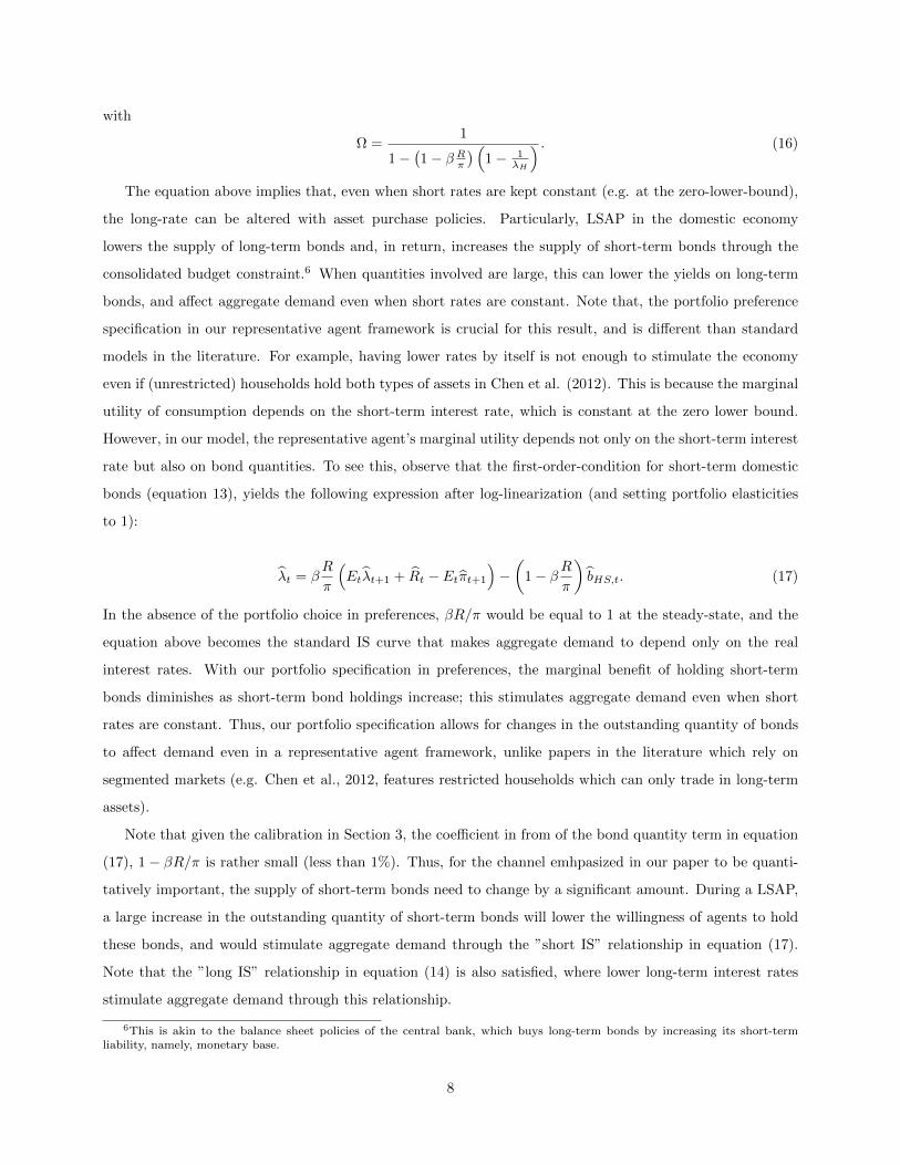
The discussion above explains the domestic transmission channel of asset purchase policies. International

spillovers of these policies can be illustrated through considering the optimality conditions of households with

respect to foreign short and long-term bonds:

rertλt = βEt

[λt+1rert+1

R∗tπ∗t+1

]+ξaat

∂at∂aF,t

∂aF,t∂bFS,t

, (18)

rertq∗L,tλt = βEt

[λt+1rert+1

1 + κq∗L,t+1

π∗t+1

]+ξaat

∂at∂aF,t

∂aF,t∂bFL,t

, (19)

where bFS,t = BFS,t/P∗t , bFL,t = BFL,t/P

∗t , and the real exchange rate rert = etP

∗t /Pt. Note that the

first-order conditions for short-term domestic and short-term foreign bonds can be combined to yield a short-

term uncovered interest parity (UIP) condition. After log-linearization (and assuming unit elasticities of

substitution in the nested CES for portfolio preference), this short-term UIP condition is given by

Rt − R∗t = Etdt+1 +

(1 − βRπβRπ

)[bHS,t −

(rert + bFS,t

)], (20)

where dt = et− et−1 denotes the nominal depreciation rate of domestic currency. The above condition implies

that the country risk-premium is determined by the quantity of outstanding short-term home and foreign

bonds. Thus, even when short-term rate differentials cannot change due to the zero lower bound, quantity

policies can still affect the exchange rate through the country risk-premium. Specifically, QE in the foreign

country leads to a higher supply of short-term foreign bonds, increasing domestic holdings of short-term

foreign bonds relative to the short-term home bonds. Higher relative holdings of short-term foreign bonds in

the home country puts downward pressure on short rates and upward pressure on the currency.7

Similarly, the first-order conditions for the long-term home and foreign bonds can be combined to yield a

long-term UIP condition, as follows:

RLRL,t − κEtRL,t+1

RL − κ−RLR

∗L,t − κEtR

∗L,t+1

RL − κ= Etdt+1 +

(1 − βRπβRπ

)[qL,t + bHL,t − (rert + q∗L,t + bFL,t)

]which suggests that the appreciation of the home currency depends on both the long-rate differential and

also the relative holdings of foreign long-term bonds.8 In Section 4, we show that the degree of appreciation

depends on the share of long-term bonds in the foreign sub-portfolio. When the domestic country holds more

long-term bonds, the percentage change in short-term bonds is larger after a LSAP in the foreign economy,

which results in a larger appreciation of the domestic currency through the short-term UIP. Since the long-

term bond share is large, the percentage change in foreign long-term bonds is smaller; thus, the effect of

7Here we discuss the spillover effects of a QE done in the foreign economy without loss of generality. Similar effects occur tothe foreign economy when the domestic economy performs QE.

8Note that the expression on the left had side of the equation reflects the expected return of selling current long-term bondsin the next period.

9

the cross-regional long-rate differentials on the exchange rate dominates the effect coming from relative bond

holdings. Thus, the long-term UIP condition also validates higher appreciation of the domestic currency in

equilibrium.

2.2 Final goods aggregators

There are two types of final goods aggregators; for consumption goods, ct, and for investment goods, it. In

what follows, we mainly describe the consumption goods aggregators, but investment goods aggregators are

modeled in an analogous fashion.

Consumption aggregators are perfectly competitive, and they produce the final goods as a CES aggregate

of home and foreign goods, ch,t and cf,t:

ct =

[γ

1λcc c

λc−1λc

h,t + (1 − γc)1λc c

λc−1λc

f,t

] λcλc−1

, (21)

where γc denotes the share of domestic goods, and λc is the elasticity of substitution between home and

foreign goods, in the consumption aggregate. For any level of output, their optimal demand for the domestic

and imported goods are given by

ch,t =

(Ph,tPt

)−λcγcct and cf,t =

(Pf,tPt

)−λc(1 − γc) ct, (22)

where Ph,t and Pf,t are the prices of the home and foreign goods, respectively. The aggregate price index for

consumption goods is given by

Pt =[γcP

1−λch,t + (1 − γc)P

1−λcf,t

] 11−λc

. (23)

The analogous expressions for investment goods aggregators (which are of measure γt in period t) are

given by:

it =

[γ

1λii i

λi−1

λi

h,t + (1 − γi)1λi i

λi−1

λi

f,t

] λiλi−1

, (24)

ih,t =

(Ph,tP it

)−λiγiit and if,t =

(Pf,tP it

)−λi(1 − γi) it, (25)

Pi,t =[γiP

1−λih,t + (1 − γi)P

1−λif,t

] 11−λi

. (26)

10

2.3 Domestic Firms

There is a unit measure of monopolistically competitive domestic firms indexed by j. Their technology is

described by the following production function:

yt (j) = [ut (j) kt−1 (j)]α

[nt (j)]1−α − f, (27)

where α is the share of capital, ut is the capital utilization rate, and f is a fixed cost of production.9

Domestic goods produced are heterogeneous across firms, and are aggregated into a homogenous domestic

good by perfectly-competitive final goods producers using a standard Dixit-Stiglitz aggregator. The demand

curve facing each firm is given by

yt (j) =

(Ph,t (j)

Ph,t

)−Θh

yt, (28)

where yt is aggregate domestic output, and Θh is the elasticity of substitution between differentiated goods

implying a gross mark up of price over marginal cost, θh = Θh /(Θh −1).

Firm j’s profits at period t is given by

Πh,t (j)

Pt=Ph,t (j)

Ptyt (j) − Wt

Ptnt (j) − rk,tkt−1 (j)

− κu1 +$

[ut (j)

1+$ − 1]kt−1 (j) − κph

2

(Ph,t (j) /Ph,t−1 (j)

πςhh,t−1π1−ςh

− 1

)2Ph,tPt

yt, (29)

where κu and $ are the level and elasticity parameters for the utilization cost. Similar to wage-stickiness,

price-stickiness is introduced via quadratic adjustment costs with level parameter κph, and ςh captures the

extent to which price adjustments are indexed to past inflation.

A domestic firm’s objective is to choose the quantity of inputs and output, and the price of its output

each period to maximize the present value of profits (using the households’ stochastic discount factor) subject

to the demand function they are facing with respect to their individual output from the aggregators. The

first-order-conditions of the firm with respect to labor and capital can be combined to relate the capital-labor

ratio to the relative price of inputs as

wt − rk,t = ut + kt−1 − nt. (30)

The first-order conditions for capital and utilization can be combined to yield

ut =1

$rk,t. (31)

Finally, the first-order-condition with respect to price yields the New Keynesian Phillips curve in domestic

9The fixed cost parameter f is set equal to θh − 1 times the steady-state level of detrended output to ensure that pureeconomic profits are zero at the steady-state; hence, there is no incentive for firm entry and exit in the long-run.

11

prices as:

πh,t =ςh

1 + ςhβπh,t−1 +

β

1 + ςhβEtπh,t+1 −

Θh − 1

(1 + ςhβ)κph

[ph,t + zt + α

(ut + kt−1 − nt

)− wt

]. (32)

2.4 Importers

There is a unit measure of monopolistically competitive importers indexed by j. They import foreign goods

from abroad, differentiate them and mark-up their price, and then sell these heterogenous goods to perfectly

competitive import aggregators, who aggregate these into a homogenous import good using a standard Dixit-

Stiglitz aggregator. The demand curve facing each importer is given by

yf,t (j) =

(Pf,t (j)

Pf,t

)−Θf

yf,t, (33)

where yf,t is aggregate imports, and Θf is a time-varying elasticity of substitution between the differentiated

goods implying a gross mark-up of the domestic price of imported goods over its import price θf = Θf/(Θf−1).

Importers maximize the present value of profits (using the households’ stochastic discount factor) subject

to the demand function they are facing from the aggregators with respect to their own output. The importer’s

profits at period t are given by:

Πf,t (j)

Pt=Pf,t (j)

Ptyf,t (j) −

etP∗h,t

Ptyf,t (j) − κpf

2

(Pf,t (j) /Pf,t−1 (j)

πςff,t−1π

1−ςf− 1

)2Pf,tPt

yf,t, (34)

where importers face quadratic price adjustment costs, which helps generate partial exchange rate pass-

through to domestic prices. κpf and ςf are the price adjustment cost and indexation parameters respectively.

The first-order condition of importers with respect to price yields the imported-price New Keynesian

Phillips curve (after log-linearization)

πf,t =ςf

1 + ςfβπf,t−1 +

β

1 + ςfβEtπf,t+1 −

Θf − 1

(1 + ςfβ)κpf

(pf,t − rert − p∗h,t

), (35)

where πf,t = Pf,t/Pf,t−1 is the import-price inflation factor.

The balance of payments identity in the model is given by(etBFS,tPt

−etR∗t−1BFS,t−1

Pt

)+

(etq∗L,tBFL,t

Pt−etR∗L,tq

∗L,tBFL,t−1

Pt

)−(B∗FS,tetPt

−Rt−1B

∗FS,t−1

etPt

)−(qL,tB

∗FL,t

etPt−RL,tqL,tB

∗FL,t−1

etPt

)=Ph,tPt

y∗f,t −etP

∗h,t

Ptyf,t. (36)

2.5 Capital producers

Capital producers are perfectly competitive. After goods production takes place, these firms purchase the

undepreciated part of the installed capital from entrepreneurs at a relative price of qt, and the new capital

12

investment goods from final goods firms at a price of Pi,t, and produce the capital stock to be carried over to

the next period. This production is subject to adjustment costs in the change in investment, and is described

by the following law-of-motion for capital:

kt = (1 − δ) kt−1 +

[1 − ϕ

2

(itit−1

− 1

)2]it, (37)

where ϕ is the adjustment cost parameter.

After capital production, the end-of-period installed capital stock is sold back to entrepreneurs at the

installed capital price of qt. The capital producers’ objective is thus to maximize

E0

∞∑t=0

βtλtλ0

[qtit − qt

ϕ

2

(itit−1

− 1

)2

it −Pi,tPt

it

], (38)

subject to the law-of-motion of capital, where future profits are again discounted using the patient households’

stochastic discount factor. The first-order-condition of capital producers with respect to investment yields

the following investment demand equation (after log-linearization):

it − it−1 = βEt

[it+1 − it

]+

1

ϕ(qt − pi,t) . (39)

2.6 Monetary and fiscal policy

The central bank targets the nominal interest rate using a Taylor rule

logRt = ρ logRt−1 + (1 − ρ)

(logR+ rπ log

πtπ

+ ry logyty

+ r∆y logytyt−1

)+ εr,t, (40)

where R is the steady-state value of the (gross) nominal policy rate, ρ determines the extent of interest rate

smoothing, and the parameters rπ, ry, and r∆y determine the importance of inflation, output gap and output

growth in the Taylor rule. y is the detrended steady-state level of output, and εr,t is a monetary policy shock

which follows an AR(1) process.

The consolidated government budget constraint is given by

gt +Rt−1

πtbS,t−1 +

RL,tπt

qL,tbL,t−1 =TAXt

Pt+ bS,t + qL,tbL,t, (41)

where bS and bL represent total short-term and long-term goverment debt, respectively. Lump-sum taxes

adjust with the level of government debt to rule out a Ponzi scheme for the government:

TAXt

Pt= Ξy

(yty

)τy (bS,t−1 + qL,t−1bL,t−1

bS + qLbL

)τb, (42)

where Ξ is a level parameter, τy is the automatic stabilizer component of transfers, and τb determines the

response of transfers to total government debt.

13

Finally, government controls the supply of long-term bonds in real terms following an AR(1) process:

log (qL,tbL,t) = (1 − ρb) log (qLbL) + ρb log (qL,tbL,t−1) + εb,t

where ρb governs the persistence of market-value of long-term bonds and εb,t represents the unconventional

monetary policy shock (i.e., QE shock) in the model.

2.7 Market clearing conditions

The domestic goods are used in the final goods production for consumption, investment, government expen-

diture, and exports:10

ch,t + ih,t + gt + y∗f,t = yt. (43)

Similarly, the imported goods are used only for consumption and investment; hence:

cf,t + if,t = yf,t. (44)

The model’s equilibrium is defined as prices and allocations such that households maximize discounted

present value of utility, all firms maximize discounted present value of profits, subject to their constraints,

and all markets clear.

3 Calibration

In our benchmark calibration, we set the structural parameters of both countries to equal values, except for

the portfolio and labor level parameters in preferences, as well as the tax level parameter in the tax policy

function.11 We calibrate the parameters using steady-state relationships in the model and US data from

the National Income and Product Accounts (NIPA; Bureau of Economic Analysis) and the Flow of Funds

Accounts (FOF; Federal Reserve Board) averaged over the post-war period.12 We first discuss the choice of the

parameters governing portfolio and preferences, and then parameters related to technology and government

policy. A list of parameter values is given in Table 1.

Portfolio. We calibrate the share of short-term assets in the domestic sub-portfolio, γH , to 0.66 based on

US residents’ portfolio share in short-term government liabilities (see Figure 2). Short-term bonds include

privately held marketable U.S. treasury securities with a remaining maturity of less than one year and the

monetary base (i.e., financial institutions’ reserves at the Federal Reserve System, vault cash and currency

10Note that utilization costs and financial costs are modeled as transfer payments to households.11A non-zero net-foreign-asset position requires these parameters to be different across regions. See below for detailed infor-

mation on these parameters.12For portfolio parameters, we use data averaged over 2000-2010 as in Figure 2 reflecting more recent government bond supply

and international developments in the financial markets.

14

outside banks) as in Chen et al. (2012). Monetary base is included since it is a perfect substitute for short

term T-bills under the zero lower bound. The short-term asset share in the foreign asset sub-portfolio, γF ,

is calibrated to 0.36 based on FOF data (see table for the Rest of the World Accounts). Foreign holdings of

short-term bonds include U.S. treasury securities with a remaining maturity of less than one year and U.S.

dollar currency.13 We assume only U.S. bonds are traded internationally, therefore, the share of the domestic

sub-portfolio for the US, γUSA , is set to 1. As for the share of domestic-asset portfolio in the ROW’s total

portfolio, γROWA , we calculate it using the ratios in Figure 2. ROW holdings of both short and long-term US

government liabilities is around 7% of their GDP (i.e., world GDP excluding the U.S. GDP). Their domestic

government bond holdings are assumed to be the same as that of US residents, i.e. around 21% of US GDP.

This implies a share of domestic-asset portfolio of 0.75 for the ROW. All elasticity of substitution parameters

in the nested CES specification for portfolio choice are set to unity. We do sensitivity analyses on these

parameters below. The coupon rate on long-term bonds, κ, is calibrated to imply a duration of 30 quarters

for long-term bonds, similar to the average duration of 10-year US Treasury bills in the secondary market.

Preferences. We calibrate the time discount factor, β, to match a target capital-output ratio, k/y, of

10 using the the optimality condition for household’s capital decision at the steady-state. Traditionally,

the discount factor is calibrated to match steady-state interest rates using the short-term bond first-order

condition. However, we use this condition to calibrate the portfolio level coefficient, ξa, in preferences using

a/y ratios both in the US and the ROW: 0.05 and 0.04 in the ROW and in the US, respectively. Since

ROW holds a higher level of government assets as a proportion of its output, its portfolio level coefficient is

calculated to be larger than in the US. We set the habit parameter, ζ, to 0.70, close to values found in Smets

and Wouters (2007) and Adolfson et el. (2008). The Frisch elasticity of labor supply, 1/ϑ, is set to 1. This

value is in line with the estimates presented in Blundell and Macurdy (1999), and represents a compromise

between the estimates in the Real Business Cycle and New Keynesian literatures (Smets and Wouters, 2007).

Labor coefficient, ξn, is calibrated to 32% to match working hours as a ratio of non-sleeping hours of the

economically active population. Note that a non-zero trade balance requires consumption-output ratio or

investment-output ratio to be different in the two regions when the same home bias parameters are assumed

in both regions’ aggregator functions. We choose, c/y, to be different across regions, which implies a different

labor level coefficient in preferences based on the optimal labor supply at the steady state.

Technology. We calibrate the capital share in home goods production, α, to 0.34 in order to match a labor

income share of 66%. Depreciation rate, δ, is calibrated to match an investment-output ratio, i/y, of 19%.

Home-bias parameters in the consumption and investment aggregators are both set to 0.9, implying a 10%

13FOF data reports holdings of US treasury securities with the original maturity. We adjust them so that short-term holdingsinclude long-term securities with a remaining maturity of less than one year using the Treasury data on the maturity of privately-held treasury securities. When distributing long-term securities with a remaining maturity of less than one year over ROW andUS residents, we use the weights in holdings of treasury bills (i.e., original maturity of less than one year) from FOF tables.

15

of import (and export) to output ratio along the steady state. Elasticity of substitution parameters in these

aggregatoes are similar to those used in New-Keynesian DSGE literature (see Gertler et al., 2007). Similarly,

the mark up and indexation parameters in the labor and goods markets (both for domestic producers and

importers) are set using values in the literature.14

Adjustment cost parameters on prices and wages, κph, κpf , κw, are calibrated so that the resulting New

Keynesian Phillips curves have slopes equivalent to assuming Calvo probabilities of 0.9 and 0.85 for wages

and prices, respectively. Investment adjustment cost parameter, ϕ, is calibrated so that investment is 2.5

times more volatile than output with a standard monetary policy shock. The capacity utilization elasticity,

$, is set to 0.12, while the adjustment cost level parameter on utilization, κu, is calibrated to imply a unit

utilization rate at the steady-state without loss of generality.

Government Policy. Taylor Rule parameters are set to values close to those found in the literature (see

Smets and Wouters, 2007 and Adolfson et el., 2008). The interest rate smoothing parameter, ρ, is set to

0.75, and inflation sensitivity, rπ is set to 1.75. The literature typically finds small response coefficients for

output gap and output growth. Thus, we set these to 0.05 in our benchmark calibration. We set the elasticity

parameters in the tax function, τy and τb, large enough to ensure a sustainable debt path (see Chen et al.,

2012). We make sure that debt converges within 10 years. The tax level parameters in the two countries,

ΞROW and ΞUS , are calibrated to match a steady state annualized interest rate of 4.4% using the government

budget constraint expression. Note that these parameters have to be different across the two regions since

we have different consumption-output ratios to match a non-zero trade balance. The resulting government-

output ratios are 17% and 18% for the ROW and the U.S., and the tax level parameters are 0.17 and 0.19

for the ROW and the U.S., respectively.

4 Results

In this section, we first use our model to evaluate the impact of QE on both domestic and foreign activity.

We then compare the spillover effects of QE in the U.S. (foreign economy) to the rest of the world (domestic

economy) with those from conventional policy.15

4.1 The impact of a QE shock

The QE shock is calibrated to match $600 billion drop in the privately-held long-term US government bonds

similar to the purchase amount announced for LSAP2 in the last quarter of 2010. Following Chen et al.

(2012), we assume no change in interest rates for four quarters after the asset purchase announcement, after

14Note that we have conducted sensitivity analysis using different values for these parameters. Their effect on key results isonly modest compared to the portfolio parameters.

15We use a first-order approximation of the model to obtain our results and use IRIS routines for all simulations.

16

which the central bank keeps its balance sheet size constant for eight quarters and then gradually sells these

bonds over the next eight quarters. The assumption of no change in interest rates in the first four quarters

following the LSAP announcement is consistent with survey evidence from Blue Chip in 2011 (Chen et al.,

2012). Note that the whole path of the aformentioned QE policy is known by all agents at the impact period.

Figure 3 shows the impulse responses of U.S. variables after a QE shock in the US. Due to imperfect

substitution between domestic short and long-term bonds, long rates in the U.S. fall by slightly more than

45 bps consistent with estimates found for LSAP2.16 Short-term bond holdings of U.S. residents increase as

well. Lower long rates and higher short holdings stimulate aggregate demand through the long and short IS

curves, respectively. As mentioned in Section 2, we do not need restricted households in our set-up, unlike

Chen et al. (2012), since the increase in the quantity of short-term holdings of the representative household

lowers the marginal benefit of holding short-term bonds even when short-term rates are fixed. This leads

to households switching expenditures to consumption and investment stimulating aggregate demand. GDP

increases by 1.4% due to the increase in consumption, investment and the improvement in the trade balance.

The trade balance improves mainly due to the increase in exports as a result of the 4.0% depreciation in the

U.S. dollar, while the immediate impact on imports is insignificant as income and price effects offset each

other.

The impulse responses of the ROW variables are shown in Figure 4. The international effects of the QE

spill over to the other country mainly through the short and long-term UIP conditions. QE generates a cross-

country differential in long-term rates at impact, which puts downward pressure on ROW long-term rates and

appreciation pressures on its currency (see the long-term UIP condition). The resulting appreciation also has

to satisfy the short-term UIP condition. Although short-term rates are not changing in the US, the quantities

would matter for the exchange rate and the ROW short-term rate. The relative increase in ROW holdings of

short-term U.S. bonds pushes the value of the ROW currency upwards, consistent with the direction implied

by the long-term UIP condition. As a result, the ROW currency appreciates, which leads to lower inflation

in the ROW, which in turn leads to a decline in current and expected short-term (policy) rates in the ROW

economy. Long rates fall by 5.5 bps in the ROW as a result of these expectations. The declines in short and

long-term rates generate increases in consumption and investment through the IS equations.17

Appreciation of the ROW currency, along with an increased demand for consumption and investment, in-

creases imports in the ROW. As mentioned earlier, U.S. demand for ROW goods does not change significantly

on impact. This results in lower net exports for ROW putting a negative pressure on their GDP. However,

16D’Amico et al. (2011) find a 55 bps decrease in 10-year Treasury bills due to LSAP2, while Krisnamurthy and Vissing-Jorgensen (2011) find 33 bps. See Bernanke (2012) for more on the effects of LSAP2 in the US.

17Here we focus on the dynamics of the model when the other region is not constrained in terms of its conventional monetarypolicy. This is consistent with the fact that emerging markets and many major advanced economies including euro-area countrieswere not facing the zero lower bound at the time of QE2. When the ROW is also assumed to face the zero lower bound fourperiods as in the U.S., the spillover effects on ROW output and long-term yields are mitigated. In that case, ROW currencyappreciates more, by 4.5%, long-term yields on ROW assets fall less, by 3 bps, and their GDP increases less, by 0.15%.

17

stimulus coming from the domestic channel in the ROW dominates the fall in net exports, and generates an

overall increase in output. These quantitative results highlight that QE spillover from the U.S. to the ROW

economy is mainly through financial channels, and not through the trade channel (i.e., not through higher

demand for ROW goods). Finally, similar to the U.S. responses, ROW starts to hold more short-term bonds

and less long-term U.S. bonds.

The result of increased US short-term bond holdings in the ROW merits some discussion. Note that even

though the ROW has a flexible exchange rate regime (i.e., does not conduct any foreign exchange intervention

to offset the currency appreciation pressures during the U.S. QE), the imperfect substitution between assets

leads the ROW agents to increase short-term U.S. bond holdings. If fixed or managed exchange rate regimes

are considered, the results on short holdings would potentially be amplified. In the extreme case of fixed

exchange rates, the ROW long-term rates would fall even more, which would necessitate larger decreases in

current and expected short rates. As U.S. short rates are fixed, through the short UIP condition, this is only

possible when there are further increases in U.S. short-term bond holdings in the ROW. The quantitative

effects of such a regime, and reserve accumulation in U.S. bonds due to this type of policy, is beyond the

scope of this paper and is left for future research.

4.2 QE shock versus interest rate shock

The direction of above-mentioned spillovers are consistent with the responses of standard interest rate cuts in

the US. We now compare quantitative differences between the spillovers from a QE shock and a conventional

interest rate shock. For comparison, we scale the interest rate shock to give the same output response that

QE shock delivers, which is around 1.4% of steady-state GDP. Table 2 compares these shocks in our model, as

well as a modified version of our model with a lower long-term bond share in ROW’s foreign-asset portfolio.

In our baseline model, the QE shock implies an increase in the ROW economic activity that is twice as

high as that implied from an interest rate shock. The depreciation of the U.S. dollar under the QE shock is

also larger than that under the interest rate shock, and ROW long-term rates fall more under the QE shock

as well. These amplified spillovers are mainly driven by the larger decrease in U.S. long-term rates after

the QE shock. The interest rate shock has a smaller impact on the long-term rates since its bond quantity

implications on the ”long IS curve” are not as severe as QE policy. Therefore, the long-term interest rate

differential between regions is higher under QE shock, which results in higher spillovers compared to interest

rate shock through the long UIP condition.

As can be observed from the last two columns of Table 2, if the share of long-term bonds in the ROW’s

foreign portfolio were smaller, the QE shock starts to act more similar to an interest rate shock. In the

next section, we conduct sensitivity analysis by considering different parameter values for the long-term bond

shares in the ROW’s foreign portfolio as well as different values for the elasticities between assets in the

18

portfolio specification.

5 Sensitivity Analysis

5.1 The share of long-term bonds in the foreign-asset portfolio

Figure 5 shows the domestic effects and the international spillover effects of QE with extreme values for the

share of long-term bonds in the ROW’s foreign-asset portfolio. As the ROW holds more long-term bonds in

their foreign portfolio in the steady-state, the effects of QE in both the U.S. and the ROW economic activities

increase. This is because the same QE shock results in higher relative supply changes in long-term bonds,

and thus lowers long rates more, as the long share increases. In the extreme case where the foreign portfolio

consists of only long-term bonds, the ROW currency appreciates by 9%, and long-term rates fall by 12 bps,

compared to 4.0% and 5.5 bps, respectively, under the baseline case. These results show that QE becomes

more effective when steady-state international holdings of U.S. long-term bonds increase.

Conversely, when ROW does not hold any long-term US government bonds, QE does not significantly

transmit cross-border, but only affects U.S. economic activity, albeit smaller than under the baseline case.

Another interesting result is that, though very small, international spillovers are not zero in this case as the

worldwide increase in the supply of short-term US bonds after QE slightly increases ROW holdings of U.S.

short-term bonds as well. This makes U.S. bonds relatively less attractive, and results in the depreciation

of the U.S. dollar through the short-term UIP condition. This special case can be seen as the isolated effect

of portfolio in preferences without the long UIP condition present in the baseline model. The fact that

international spillovers are very small in this case shows that introduction of long UIP in the model is crucial

to understand the international effects of LSAPs quantitatively.

5.2 Elasticity of substitution parameters in the portfolio specification

We now analyze the sensitivity of results to elasticity parameters in our portfolio specification. We start with

the elasticity of substitution between long-term and short-term bonds in the domestic-asset portfolio, λH .

Figure 6 shows the results for different values of λH ; namely when λ = 0.25, 1, 25.18 This figure suggests

that spillovers increase when bonds in the domestic-asset portfolio are less substitutable with each other. A

lower degree of substitution amplifies the effect of a change in the relative supply of bonds, resulting in a

larger change in the relative prices of assets and a bigger fall in long-term rates, which in turn stimulates

the domestic economy more. Foreign economic activity increases more as well through the financial channel.

Conversely, a value as large as 25 for this elasticity parameter implies almost no spillovers since short and

long-term bonds are almost perfectly substitutable.

18Since both regions hold a domestic portfolio, we change this parameter for both regions. However, as there is no QE in theROW, keeping elasticity the same in the ROW’s domestic portfolio implies similar results.

19

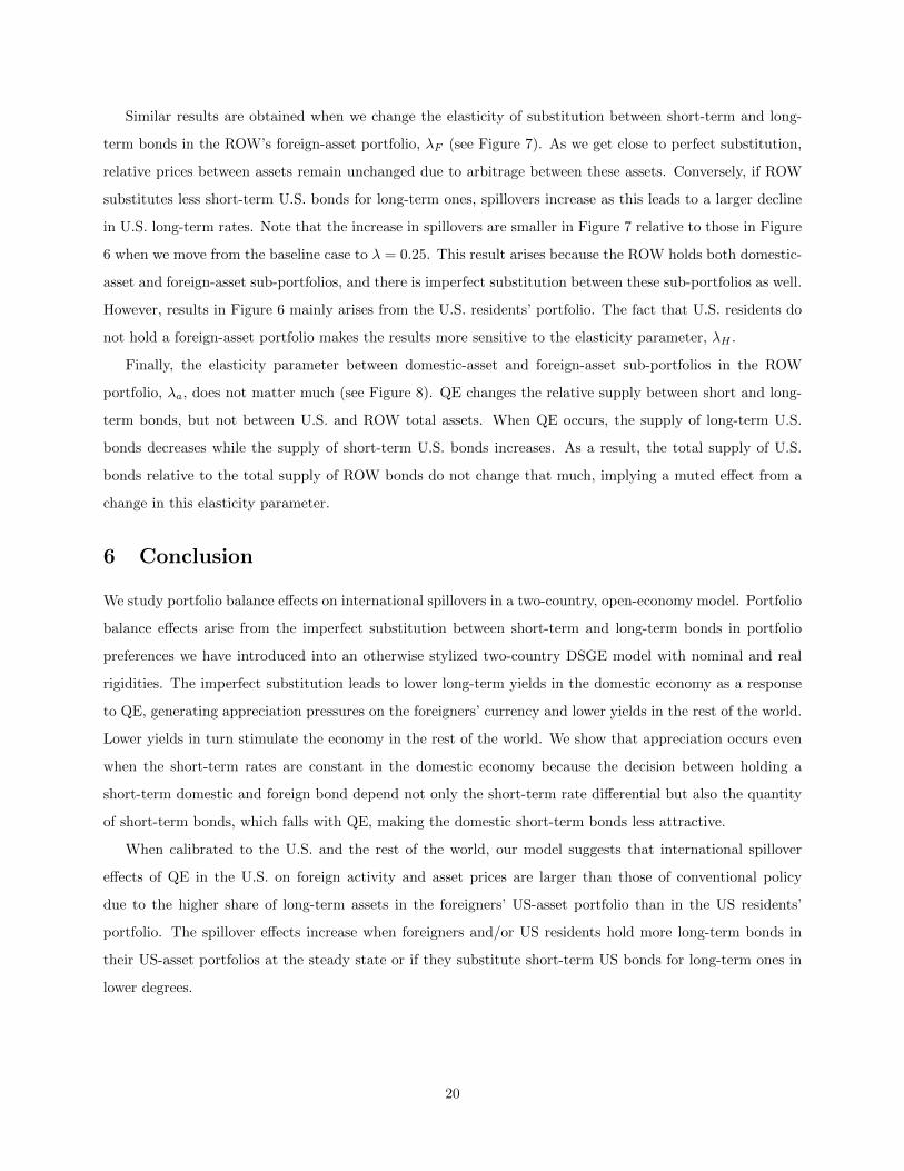
Similar results are obtained when we change the elasticity of substitution between short-term and long-

term bonds in the ROW’s foreign-asset portfolio, λF (see Figure 7). As we get close to perfect substitution,

relative prices between assets remain unchanged due to arbitrage between these assets. Conversely, if ROW

substitutes less short-term U.S. bonds for long-term ones, spillovers increase as this leads to a larger decline

in U.S. long-term rates. Note that the increase in spillovers are smaller in Figure 7 relative to those in Figure

6 when we move from the baseline case to λ = 0.25. This result arises because the ROW holds both domestic-

asset and foreign-asset sub-portfolios, and there is imperfect substitution between these sub-portfolios as well.

However, results in Figure 6 mainly arises from the U.S. residents’ portfolio. The fact that U.S. residents do

not hold a foreign-asset portfolio makes the results more sensitive to the elasticity parameter, λH .

Finally, the elasticity parameter between domestic-asset and foreign-asset sub-portfolios in the ROW

portfolio, λa, does not matter much (see Figure 8). QE changes the relative supply between short and long-

term bonds, but not between U.S. and ROW total assets. When QE occurs, the supply of long-term U.S.

bonds decreases while the supply of short-term U.S. bonds increases. As a result, the total supply of U.S.

bonds relative to the total supply of ROW bonds do not change that much, implying a muted effect from a

change in this elasticity parameter.

6 Conclusion

We study portfolio balance effects on international spillovers in a two-country, open-economy model. Portfolio

balance effects arise from the imperfect substitution between short-term and long-term bonds in portfolio

preferences we have introduced into an otherwise stylized two-country DSGE model with nominal and real

rigidities. The imperfect substitution leads to lower long-term yields in the domestic economy as a response

to QE, generating appreciation pressures on the foreigners’ currency and lower yields in the rest of the world.

Lower yields in turn stimulate the economy in the rest of the world. We show that appreciation occurs even

when the short-term rates are constant in the domestic economy because the decision between holding a

short-term domestic and foreign bond depend not only the short-term rate differential but also the quantity

of short-term bonds, which falls with QE, making the domestic short-term bonds less attractive.

When calibrated to the U.S. and the rest of the world, our model suggests that international spillover

effects of QE in the U.S. on foreign activity and asset prices are larger than those of conventional policy

due to the higher share of long-term assets in the foreigners’ US-asset portfolio than in the US residents’

portfolio. The spillover effects increase when foreigners and/or US residents hold more long-term bonds in

their US-asset portfolios at the steady state or if they substitute short-term US bonds for long-term ones in

lower degrees.

20

References

[1] Adolfson, M., Laseen, S., Linde, J., & Villani, M. (2008). Evaluating an estimated new Keynesian small

open economy model. Journal of Economic Dynamics and Control, 32(8), 2690-2721.

[2] Bauer, M. D., & Neely, C. J. (2014). International channels of the Fed’s unconventional monetary policy.

Journal of International Money and Finance (forthcoming).

[3] Baumeister, C., and Benati, L. (2013). Unconventional Monetary Policy and the Great Recession: Es-

timating the Macroeconomic Effects of a Spread Compression at the Zero Lower Bound. International

Journal of Central Banking, 9(2), 165-212.

[4] Benes, J., M. K. Johnston, and S. Plotnikov, IRIS Toolbox Release 20130208 (Macroeconomic modeling

toolbox), software available at http://www.iris-toolbox.com.

[5] Bernanke, B. S. 2012. “Monetary Policy Since the Onset of the Crisis.” Speech at the Federal Reserve

Bank of Kansas City Economic Symposium, Jackson Hole, Wyoming, 31 August.

[6] Blundell, R., & MaCurdy, T. (1999). Labor supply: A review of alternative approaches. Handbook of

labor economics, 3, 1559-1695.

[7] Chen, H., V. Curdia, and A. Ferrero (2012). ”The Macroeconomic Effects of Large-Scale Asset Purchase

Programmes,” Economic Journal, 122, F289-F315.

[8] Chen, Q, A Filardo, D He and F Zhu (2012): “International spillovers of central bank balance sheet

policies”, in “Are central bank balance sheets in Asia too large?”, BIS Papers, no 66, pp 230–74.

[9] Christiano, L. J., M. Eichenbaum, and C. L. Evans (2005). ”Nominal Rigidities and the Dynamic Effects

of a Shock to Monetary Policy,” Journal of Political Economy, 113, 1-45.

[10] Curdia, V., and M. Woodford. (2011). ”The Central Bank Balance Sheet as an Instrument of Monetary

Policy,” Journal of Monetary Economics, 58, 54-7.

[11] D’Amico, S., English, W., Lopez-Salido, D., & Nelson, E. (2012). The Federal Reserve’s Large-scale

Asset Purchase Programmes: Rationale and Effects*. The Economic Journal, 122(564), F415-F446.

[12] Dorich, J., R. Mendes, and Y. Zhang (2013). ”Quantitative Easing at the Zero Lower Bound,” mimeo,

Bank of Canada.

[13] Fratzscher, M., Lo Duca, M., & Straub, R. (2013). On the international spillovers of US quantitative

easing (No. 1304). Discussion Papers, DIW Berlin.

21

[14] Gertler, M., Gilchrist, S. and Natalucci, F.M. (2007). “External Constraints on Monetary Policy and the

Financial Accelerator,” Journal of Money, Credit and Banking, 39, 295-330.

[15] Gertler, M., and P. Karadi (2011). “A Model of Unconventional Monetary Policy,” Journal of Monetary

Economics, 58, 17-34.

[16] Harrison, R. (2012). Asset purchase policy at the effective lower bound for interest rates (No. 444). Bank

of England.

[17] Krishnamurthy, A., & Vissing-Jorgensen, A. (2011). The effects of quantitative easing on interest rates:

channels and implications for policy (No. w17555). National Bureau of Economic Research.

[18] Neely, C. J., August 2013. Unconventional monetary policy had large international effects. Working

Paper Series 2010-018E, Federal Reserve Bank of St. Louis.

[19] Rotemberg, J. J. (1982). ”Monopolistic Price Adjustment and Aggregate Output,” Review of Economic

Studies, 49, 517-31.

[20] Smets, F., and R. Wouters (2007). ”Shocks and Frictions in US Business Cycles: A Bayesian DSGE

Approach,” American Economic Review, 97, 586-606

[21] Woodford, M. (2001). Fiscal requirements for price stability (No. w8072). National Bureau of Economic

Research.

22

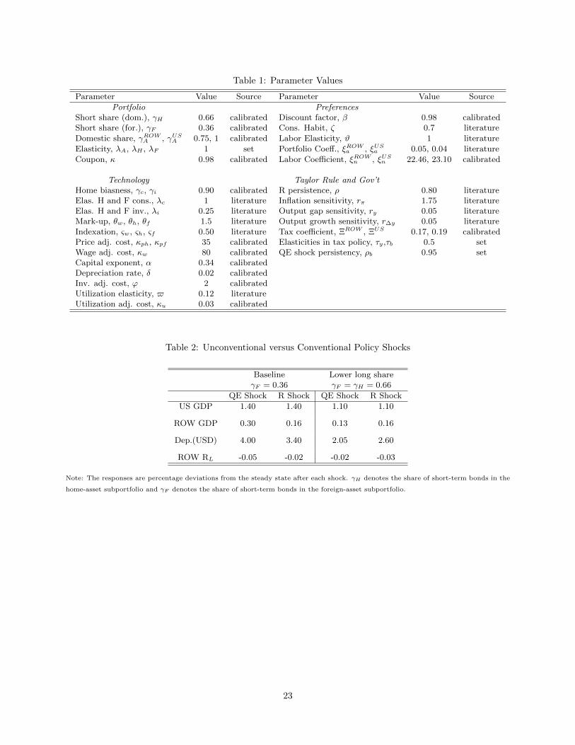
Table 1: Parameter Values

Parameter Value Source Parameter Value Source

Portfolio PreferencesShort share (dom.), γH 0.66 calibrated Discount factor, β 0.98 calibratedShort share (for.), γF 0.36 calibrated Cons. Habit, ζ 0.7 literatureDomestic share, γROWA , γUSA 0.75, 1 calibrated Labor Elasticity, ϑ 1 literatureElasticity, λA, λH , λF 1 set Portfolio Coeff., ξROWa , ξUSa 0.05, 0.04 literatureCoupon, κ 0.98 calibrated Labor Coefficient, ξROWn , ξUSn 22.46, 23.10 calibrated

Technology Taylor Rule and Gov’tHome biasness, γc, γi 0.90 calibrated R persistence, ρ 0.80 literatureElas. H and F cons., λc 1 literature Inflation sensitivity, rπ 1.75 literatureElas. H and F inv., λi 0.25 literature Output gap sensitivity, ry 0.05 literatureMark-up, θw, θh, θf 1.5 literature Output growth sensitivity, r∆y 0.05 literatureIndexation, ςw, ςh, ςf 0.50 literature Tax coefficient, ΞROW , ΞUS 0.17, 0.19 calibratedPrice adj. cost, κph, κpf 35 calibrated Elasticities in tax policy, τy,τb 0.5 setWage adj. cost, κw 80 calibrated QE shock persistency, ρb 0.95 setCapital exponent, α 0.34 calibratedDepreciation rate, δ 0.02 calibratedInv. adj. cost, ϕ 2 calibratedUtilization elasticity, $ 0.12 literatureUtilization adj. cost, κu 0.03 calibrated

Table 2: Unconventional versus Conventional Policy Shocks

Baseline Lower long shareγF = 0.36 γF = γH = 0.66

QE Shock R Shock QE Shock R Shock

US GDP 1.40 1.40 1.10 1.10

ROW GDP 0.30 0.16 0.13 0.16

Dep.(USD) 4.00 3.40 2.05 2.60

ROW RL -0.05 -0.02 -0.02 -0.03

Note: The responses are percentage deviations from the steady state after each shock. γH denotes the share of short-term bonds in the

home-asset subportfolio and γF denotes the share of short-term bonds in the foreign-asset subportfolio.

23

Figure 3: Domestic (US) Responses to a QE shock (%)

0 10 20 30 40−30

−20

−10

0

QE shock(Long−term bonds)

0 10 20 30 40−0.5

0

0.5

1

1.5Inflation

0 10 20 30 40−0.5

0

0.5

1Policy Rate

0 10 20 30 40−0.8

−0.6

−0.4

−0.2

0Long−term Rate

0 10 20 30 40−0.5

0

0.5

1

1.5GDP

0 10 20 30 40−0.5

0

0.5

1Consumption

0 10 20 30 40−2

0

2

4

6Investment

0 10 20 30 40−1

0

1

2Trade Balance

0 10 20 30 40−40

−20

0

20

U.S. residents’long−term holdings

0 10 20 30 40−10

0

10

20

U.S. residents’ short−term holdings

0 10 20 30 40−2

0

2

4USD depreciation

TBExportsImports

Figure 4: ROW Responses to a QE Shock (%)

0 10 20 30 40−2

0

2

4Appreciation

0 10 20 30 40−0.4

−0.2

0

0.2

0.4Inflation

0 10 20 30 40−0.3

−0.2

−0.1

0

0.1Policy Rate

0 10 20 30 40−0.06

−0.04

−0.02

0

0.02Long−term Rate

0 10 20 30 40−0.2

0

0.2

0.4

0.6GDP

0 10 20 30 400

0.05

0.1

0.15

0.2Consumption

0 10 20 30 40−1

0

1

2Investment

0 10 20 30 40−2

−1

0

1

2Trade Balance

0 10 20 30 40−20

−10

0

10

ROW holdings oflong−term US bonds

0 10 20 30 40−20

0

20

40

60

ROW holdings ofshort−term US bonds

TBExportsImports

24

Figure 5: Results of Different Shares of US Long-term bonds in the ROW Foreign-asset portfolio (%)

0 10 20 30 40−1

0

1

2

3GDP

US

0 10 20 30 40−1

0

1

2Inflation

0 10 20 30 40−0.5

0

0.5

1

1.5Policy Rate

0 10 20 30 40−1

−0.5

0Long−term Rate

0 10 20 30 40−0.5

0

0.5

1GDP

RO

W

0 10 20 30 40−1

−0.5

0

0.5Inflation

0 10 20 30 40−1

−0.5

0

0.5Policy Rate

0 10 20 30 40−0.15

−0.1

−0.05

0

0.05Long−term Rate

0 10 20 30 40−5

0

5

10RER (USD Depr.)

All longBaselineAll short

Figure 6: Results of Different Elasticity of Substitution between (domestic) ST and LT bonds (%)

0 10 20 30 40−2

0

2

4GDP

0 10 20 30 40−1

0

1

2

3Inflation

0 10 20 30 40−0.5

0

0.5

1

1.5Policy Rate

0 10 20 30 40−1.5

−1

−0.5

0Long−term Rate

0 10 20 30 40−0.5

0

0.5

1GDP

0 10 20 30 40−1

−0.5

0

0.5Inflation

0 10 20 30 40−0.6

−0.4

−0.2

0

0.2Policy Rate

0 10 20 30 40−0.15

−0.1

−0.05

0

0.05Long−term Rate

0 10 20 30 40−5

0

5

10RER (USD Depr.)

λH

=0.25

λH

=1

λH

=25

25

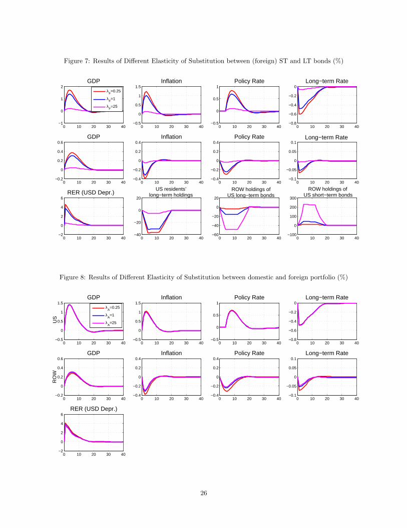
Figure 7: Results of Different Elasticity of Substitution between (foreign) ST and LT bonds (%)

0 10 20 30 40−1

0

1

2GDP

0 10 20 30 40−0.5

0

0.5

1

1.5Inflation

0 10 20 30 40−0.5

0

0.5

1Policy Rate

0 10 20 30 40−0.8

−0.6

−0.4

−0.2

0Long−term Rate

0 10 20 30 40−0.2

0

0.2

0.4

0.6GDP

0 10 20 30 40−0.4

−0.2

0

0.2

0.4Inflation

0 10 20 30 40−0.4

−0.2

0

0.2

0.4Policy Rate

0 10 20 30 40−0.1

−0.05

0

0.05

0.1Long−term Rate

0 10 20 30 40−2

0

2

4

6RER (USD Depr.)

0 10 20 30 40−40

−20

0

20

US residents’long−term holdings

0 10 20 30 40−60

−40

−20

0

20

ROW holdings ofUS long−term bonds

0 10 20 30 40−100

0

100

200

300

ROW holdings of US short−term bonds

λF=0.25

λF=1

λF=25

Figure 8: Results of Different Elasticity of Substitution between domestic and foreign portfolio (%)

0 10 20 30 40−0.5

0

0.5

1

1.5GDP

US

0 10 20 30 40−0.5

0

0.5

1

1.5Inflation

0 10 20 30 40−0.5

0

0.5

1Policy Rate

0 10 20 30 40−0.8

−0.6

−0.4

−0.2

0Long−term Rate

0 10 20 30 40−0.2

0

0.2

0.4

0.6GDP

RO

W

0 10 20 30 40−0.4

−0.2

0

0.2

0.4Inflation

0 10 20 30 40−0.4

−0.2

0

0.2

0.4Policy Rate

0 10 20 30 40−0.1

−0.05

0

0.05

0.1Long−term Rate

0 10 20 30 40−2

0

2

4

6RER (USD Depr.)

λA=0.25

λA=1

λA=25

26