Multiple Viewpoint Systems: Time Complexity

and the Construction of Domains for

Complex Musical Viewpoints in

the Harmonisation Problem

Raymond P. Whorley1, Geraint A. Wiggins2,Christophe Rhodes1, and Marcus T. Pearce2

1 Department of ComputingGoldsmiths, University of London

New Cross, London SE14 6NW, UK2 School of Electronic Engineering and Computer Science

Queen Mary, University of LondonMile End Road, London E1 4NS, UK

Abstract. We discuss the problem of automatic four-part harmonisa-tion: given a soprano part, add alto, tenor and bass in accordance withthe compositional practices of a particular musical era. In particular, wefocus on the development of representational and modelling techniques,within the framework of multiple viewpoint systems and Prediction byPartial Match (PPM), for the creation of statistical models of four-partharmony by machine learning. Our ultimate goal is to create better mod-els, according to the information theoretic measure cross-entropy, thanhave yet been produced. We use multiple viewpoint systems because oftheir ability to represent both surface and underlying musical structure,and because they have already been successfully applied to melodic mod-elling. To allow for the complexities of harmony, however, the frameworkmust be extended; for example, we begin by predicting complete chords,and then extend the framework to allow part by part prediction. Asthe framework is extended and generalised, the viewpoints become morecomplex. This article discusses matters related to viewpoint domains(alphabets), such as their size and consequent effect on run time; andpresents methods for their reliable construction. We also present an em-pirical analysis of the time complexity of our computer implementation.

1 Introduction

We are attempting to solve by computational means the problem of automaticfour-part harmonisation: given a soprano part, add alto, tenor and bass in ac-cordance with the compositional practices of a particular musical era. Multipleviewpoint systems were introduced by Conklin and Cleary (1988), who used themto hand-craft some simple statistical models of polyphony. Their application tomelody (Conklin, 1990; Conklin and Witten, 1995) was more successful, culmi-nating in the work of Pearce and Wiggins (2006, 2012), who demonstrated that

2

statistical models such as these can successfully model listeners’ expectations.Conklin (2002) used viewpoints (although not multiple viewpoint systems per se)to discover repeatedly occurring harmonic patterns in a corpus of music. In thisarticle we are concerned with the extension of this framework to the harmonicdomain, given its promising melodic results and obvious potential in the field ofharmony. In particular, we are focusing on the development of representationaland modelling techniques, within the framework of multiple viewpoint systemsand Prediction by Partial Match (PPM, Cleary and Witten, 1984), for the cre-ation of statistical models of four-part harmony by machine learning. Our aimis to create better statistical models of harmony, according to the informationtheoretic measure cross-entropy (see §3.7), than have so far been produced. Aprimitive viewpoint describes a single feature of a sequence of musical objects;in this case, the objects are concurrently sounding notes. An example of a view-point employed in the modelling of music is Pitch. In this and earlier relatedresearch (Conklin and Witten, 1995; Pearce and Wiggins, 2004), the set of validelements (or symbols, or values) for this viewpoint, its domain, comprises pitchvalues represented as MIDI numbers. This article addresses three fundamentalissues relating to domains, illustrating the fact that extending the multiple view-point framework to harmony is non-trivial. One issue is the size of the Pitch

domain; to predict all possible SATB note combinations, the domain is so largethat prediction is excessively slow (we carry out a time complexity analysis in§9). We discuss principled ways of reducing the domain size, such that reason-able running times are made possible. Another issue is whether or not a domaincan be fixed at the beginning of the prediction process, such that it can be usedunchanged at all positions in a musical sequence. We explain why this is not,in general, possible. Finally, we see that the construction of domains for linkedviewpoints (viewpoints formed by combining two or more primitive viewpoints)is far from straightforward. We show how to reliably construct linked viewpointdomains of various complexities, and explain why this is important.

§3 provides a brief description of multiple viewpoint systems and associatedmodelling techniques; §4 gives a very short description of our corpus and testdata; §5 introduces domain-related issues by considering melodic viewpoint do-mains; and §§6–8 deal with the viewpoint domains of versions 1, 2 and 3 of ourframework for modelling harmony respectively (having first introduced theseversions). A procedure for the construction of complex viewpoint domains isoutlined in the latter section, along with a detailed example. This procedure isformally presented as algorithms in Appendix A, which includes a line-by-linedescription following the same detailed example. There is an analysis of the timecomplexity of our computer model in §9, and in §10 we examine four hymn tuneharmonisations automatically generated by our best model to date. Finally, westate our conclusions and indicate the direction of our future work in §11; butfirst, we review the relevant literature.

3

2 Previous Approaches to the Modelling of Harmony

There have been many attempts to model musical composition, or aspects of it,using AI techniques. Modelling four-part harmony is difficult: even if we wereto encode an entire treatise on harmony into a computer system, the harmonyproduced by that system is unlikely to match that of an expert musician, whohas the advantage of having actually experienced music; that is, music alwaysgoes beyond the rules that an analyst can synthesise from it. What we wouldideally like to do is to find a way to model harmony such that the system iscapable of producing consistently good harmony in any specified style. Previousapproaches to the modelling of harmony are briefly outlined below.

Constraint-based Methods Ebcioglu (1988) describes CHORAL, a rule-based ex-pert system (using first-order logic), for the four-part harmonisation of choralemelodies in the style of J. S. Bach. The predicates are grouped in such a waythat the music is observed frommultiple viewpoints (the multiple viewpoints hereare different from those used by Conklin, 1990, not least because no statisticalmodelling is involved; although they do appear to have been the original inspira-tion). Pachet and Roy (1998) focus on the exploitation of part-whole relations;for example, the relationship between note and chord. They use object-orientedtechniques to build a structured representation of music, called the MusES sys-tem (Pachet et al., 1996), with which knowledge of harmony can be expressed.

Evolutionary Methods Phon-Amnuaisuk et al. (1999) use a genetic algorithm togenerate homophonic four-part harmony for given melodies. Phon-Amnuaisukand Wiggins (1999) compare the performance of this system with that of arule-based system into which the same amount of musical knowledge has beenencoded. An objective evaluation of the harmonisations clearly demonstrates thesuperiority of the rule-based approach, which is thought to be due to additionalimplicit knowledge in the form of a structured search mechanism.

Connectionist Methods Hild et al. (1992) have created a neural network systemcalled HARMONET, which is capable of producing four-part harmonisations ofchorale melodies in the style of J. S. Bach. A key feature of the architecture ofthis system is that the overall harmonisation task is divided into a number ofsubtasks.

Statistical Modelling Clement (1998) uses first-order N-gram models (see §3.3) todemonstrate that two distinct (though artificial) styles of harmonic progressioncan be learned. Ponsford et al. (1999) improve on this by using N-grams ofup to third-order to create statistical models of underlying harmonic movementfrom a corpus of seventeenth century French sarabandes. Biyikoglu (2003) usesN-gram models to study harmonic syntax and the relationship between melodyand harmony. Allan (2002) suggests that melody can be properly taken intoconsideration in statistical models by using N-gram models in which a contextof melody notes is added to the historical harmonic context.

4

Assayag et al. (1999) describe a dictionary-based approach to the machinelearning of music. The models they construct are similar to N-gram models inmany respects. To facilitate the modelling of polyphony, music is transformedinto a sequence of discrete events using the full expansion technique. Specialsymbols indicate notes which continue to sound from event to event.

Allan (2002) describes a harmonisation model which uses hidden MarkovModels (HMMs). Following Hild et al. (1992), the overall harmonisation taskis divided into three subtasks (Allan and Williams, 2005, merge the first twosubtasks in later work). The Viterbi algorithm (Viterbi, 1967) can be used tofind the globally most probable sequence of hidden states from an observed eventsequence. The model was evaluated by calculating cross-entropies (see §3.7).

Raphael and Stoddard (2003, p. 181) propose a Bayesian network modelfor harmonic analysis which “regards the data as a collection of voices wherethe evolution of each voice is conditionally independent of the others, given theharmonic state.”

3 The Multiple Viewpoint Framework

3.1 Motivation for the Use of Multiple Viewpoints to ModelHarmony

Ebcioglu (1988) was responsible for one of the more successful efforts at mod-elling harmony, producing an expert system which incorporated explicit hard-coded rules to encapsulate musical knowledge. There are problems associatedwith this sort of rule-based of approach, however. Firstly, for any given style ofharmonisation, there are many general rules with lots of exceptions. Formulatinga theory of a style by creating a model in this way, therefore, requires expertise,is extremely time consuming, and results in a theory which is likely to be incom-plete. Secondly, to formulate theories of different harmonic styles (e.g., those ofTallis, Bach and Mozart), it is necessary to infer different sets of general rulesand exceptions, which multiplies the time expended by the expert.

Machine learning has the potential to circumvent the above problems; thecomputer learns for itself how to harmonise in a particular style by constructinga model of harmony from a corpus of stylistically homogeneous music. Oncethe machine learning program has been written, and is demonstrably workingsatisfactorily, it should be able to model the style of harmony of any corpuspresented to it. Providing that the resulting model is able to consistently generateharmonisations which are indistinguishable (by an expert; Pearce and Wiggins,2007) in style from those in the corpus, then it is a theory of that style, containingstructure equivalent to rules and exceptions.

Later work by Allan and Williams (2005) emphatically demonstrated thepotential of a statistical machine learning approach: they used HMMs to createa model of four-part harmony from a corpus of chorale melodies harmonised byJ. S. Bach. Harmonisations generated by their model convey a definite flavourof Bach’s style, and some of them are very good; but Allan and Williams (2005)

5

themselves recognise that better modelling, possibly within the framework ofConditional Random Fields (CRFs, Lafferty et al., 2001), could improve theirharmonisations. They say that whereas their system represents chords simplyas sets of intervals, the CRF framework would allow the inclusion of additionalfeatures such as position in bar and key signature.

An established means of representing music which, when combined with ma-chine learning and modelling techniques, is able to incorporate such features (andmany others beside), is a framework calledmultiple viewpoint systems, which wasformulated in seminal work by Conklin (1990) and Conklin and Witten (1995).This not only directly represents basic musical attributes like duration and pitch,but also derived attributes such as intervals. The use of these derived attributesnecessarily introduces a certain amount of low-level musical knowledge, whichresearchers such as Dixon and Cambouropoulos (2000) have found to be bene-ficial. Pearce (2005) has successfully used this framework to produce cognitivemodels of melodic expectancy, which in turn has led to models being developedto predict phrase segmentation (Pearce et al., 2008, 2010). On the basis of itspast success in the musical sphere, we consider the multiple viewpoint frameworkto be the ideal representation scheme for the modelling of harmony.

Having motivated the representation, we now move on to the modelling.Prediction by Partial Match (PPM, Cleary and Witten, 1984) uses an escapemethod to create viewpoint prediction probability distributions from N-grammodels of different order, starting with the highest order and backing off tolower orders (see §3.3 for more details). This is where viewpoint domains comein: if a distribution does not contain all possible predictions by the time the 0th-order model has been incorporated, it is completed by backing off to a uniformdistribution comprising all of the members of the relevant domain.

We consider that the flexibility which the multiple viewpoint framework af-fords, both in terms of the number of viewpoints (and their combination) andthe ability to utilise different context sizes, gives it an advantage over methodsusing a single or very few “viewpoints,” and/or methods using a single contextsize. HARMONET (Hild et al., 1992) effectively uses four “viewpoints” linkedtogether in a predetermined way to form three different context sizes (in theadvanced system). Similarly, the Bayesian network approach described in §2(Raphael and Stoddard, 2003) uses a very limited number of “viewpoints,” andthe models are no larger than 2nd-order. The multiple viewpoint framework, onthe other hand, allows the use of a viewpoint selection algorithm to optimise themodel by choosing which of many viewpoints should be in the system, and howthey should be linked (see §3.6).

Having motivated the use of the multiple viewpoint framework, we first de-scribe multiple viewpoint systems as applied to the modelling of melody.

3.2 Viewpoint Types

A type τ is an attribute or property of an event in a sequence (here a note ina melodic sequence). Basic types are the fundamental attributes of a note thatare predicted or given. One that is predicted is Pitch, which is represented as

6

MIDI numbers in the current implementation; for example, the note G4 has aPitch value of 67. Another is Duration, which is represented using units of oneninety-sixth of a semibreve (whole note); for example, a crotchet (quarter note)has a Duration value of 24. Some basic types that are given are: the start-timeof a note (Onset); the number of flats or sharps in the key signature (KeySig),where for example 3 flats has a KeySig value of −3, and 1 sharp a value of 1;whether the melody is in a major or a minor key (Mode), where major has aMode value of 0, and minor a value of 9; and whether a note is at the beginningor end of a phrase, or otherwise (Phrase), which has possible values 1 (first notein phrase), −1 (last note in phrase) and 0 (otherwise). [τ ] denotes the set ofvalid values, symbols or elements for a viewpoint type, which in the latter caseis {−1, 0, 1}; this is called the syntactic domain, hereafter simply referred to asthe domain. There are several more basic types; but if we assume that this isthe full set of basic types, then the set of representable events (notes in the caseof melody), called the event space, is

[Onset]× [Duration]× [Pitch]× [KeySig]× [Mode]× [Phrase].

Derived types such as sequential pitch interval (Interval) and sequential du-ration ratio (DurRatio) are derived from, and can therefore predict, basic types(in this case Pitch and Duration respectively). Interval is the difference inpitch between two consecutive notes, measured in semitones (ascending inter-vals have positive values); and DurRatio is the ratio of the duration of a noteto the duration of the immediately preceding note. Derived types are not neces-sarily defined at all positions in a sequence, with both Interval and DurRatio

being undefined at the first note. An example of a viewpoint type derived fromgiven attributes is the tonic of the relevant major or minor scale (Tonic), whichis derived from KeySig and Mode; for example, when KeySig is 1 and Mode is 0(major key with 1 sharp), Tonic is G. This is used in the determination of thepitch interval from the tonic (ScaleDegree, measured in semitones), which isprimarily derived from, and can therefore predict, Pitch.

Threaded types are defined only at certain positions in a sequence, determinedby Boolean test viewpoints such as FirstInBar; for example, ScaleDegree ⊖FirstInBar has a defined ScaleDegree value only for the first note in a bar.Threaded types are able to model longer range dependencies. Basic, derived, andin this research threaded types are collectively known as primitive types. Notethat Conklin and Witten (1995) included a timescale with each threaded type,which, as Pearce (2005) pointed out, effectively meant that it was a linked type(see below). The timescale was required to predict attributes which are assumedto be given in this research.

A linked type, or product type, is the conjunction of two or more primitiveviewpoints; for example, DurRatio ⊗ Interval. If any of the constituent view-points are undefined, then the linked viewpoint is also undefined. The type set ofa type τ is denoted by 〈τ〉. This set comprises the basic types that a viewpointis able to predict (i.e., the basic types from which it is derived); therefore

〈DurRatio ⊗ Interval〉 = {Duration, Pitch}.

7

Basic: Pitch 67 67 71 69 67 69 69 71Duration 48 48 48 48 48 48 48 48

Derived: Interval ⊥ 0 4 −2 −2 2 0 2ScaleDegree 0 0 4 2 0 2 2 4

Threaded: ScaleDegree ⊖ FiB ⊥ 0 ⊥ ⊥ ⊥ 2 ⊥ ⊥Linked: DurRatio ⊗ Interval ⊥ 〈1, 0〉 〈1, 4〉 〈1,−2〉 〈1,−2〉 〈1, 2〉 〈1, 0〉 〈1, 2〉

Fig. 1. First phrase of hymn tune Luther’s Hymn (Nun freut euch) adapted fromVaughanWilliams (1933), with sequences of viewpoint elements underneath. ViewpointFirstInBar has been abbreviated to FiB. The symbol ⊥ means that a viewpoint isundefined.

Figure 1 shows the first phrase of hymn tune Luther’s Hymn (Nun freut euch)adapted from Vaughan Williams (1933), with example sequences of viewpointelements underneath. See Table 1 for the subset of viewpoint types referredto in this article and their meanings. Other than for threaded types, viewpointnomenclature in this article follows, and where necessary extends, that of Pearceand Wiggins (2006). See also Conklin and Witten (1995) and Pearce (2005) formore details.

3.3 N-gram Models

So far, N-gram models (or context models), which are Markov models employingsubsequences of N symbols, have been the modelling method of choice when us-ing multiple viewpoint systems (Conklin and Witten, 1995; Pearce, 2005). Theidea is to predict the next symbol in a sequence by taking account of the imme-diately preceding defined symbols. The transition probability of the N th symbol,the prediction, depends only upon the previous N − 1 symbols, the context. Thenumber of symbols in the context is the order of the model. Transition probabili-ties are determined by maximum likelihood estimation: see Manning and Schutze(1999) for more details.

A viewpoint model is a weighted combination of various orders of N-grammodel of a particular viewpoint type. The N-gram models can be combined by,for example, Prediction by Partial Match (PPM, Cleary and Witten, 1984). PPMmakes use of a sequence of models, which we call a back-off sequence, for contextmatching and the construction of complete prediction probability distributions(i.e., containing all possible predictions, however improbable). The back-off se-quence begins with the highest order model, proceeds to the second-highest or-der, and so on. An escape method determines weights for prediction probabilitiesat each stage in this sequence, which are generally high for predictions appearingin high-order models, and vice versa. If necessary, a probability distribution iscompleted by backing off to a uniform distribution (where the probability massis divided equally between all elements in the relevant domain). In this research,

8

Table 1. Viewpoint types τ referred to in this article.

τ Meaning Derived from

Basic

Onset start-time of eventDuration duration of eventCont event continuation, or otherwisePitch chromatic pitchKeySig number of flats or sharpsMode major or minor keyPhrase event at start/end of phrase, or not

Derived

DurRatio sequential duration ratio Duration

Interval sequential chromatic pitch interval Pitch

Tonic tonic of relevant major/minor scale KeySig, ModeScaleDegree chromatic pitch interval from tonic Pitch

FirstInBar first event in bar, or otherwise Onset

LastInPhrase last event in phrase, or otherwise Phrase

Threaded

ScaleDegree ⊖ FirstInBar ScaleDegree threaded at first in bar Pitch, Onset

we are using escape method C (see Witten and Bell, 1989, for a review of thisand other escape methods). We are also using a method known as exclusionin conjunction with escape to obtain more accurate estimates; see Cleary andTeahan (1997) for more details.

3.4 Multiple Viewpoints

A multiple viewpoint system comprises more than one viewpoint: indeed, usu-ally many more. If we were to use only unlinked basic viewpoint types to predictexisting data, it would be possible to back off under PPM until the requiredprediction (and its associated probability) was found, without needing to com-plete the distribution. In general, this is not the case, however; there may, forexample, be derived viewpoints in the system. Backing off only until the requiredprediction is found will result in different sets of predictions in the respective dis-tributions (once they have been converted into distributions over the domain ofthe basic type), which makes it impossible to properly combine the distributionsso that the overall prediction probability can be found. This, fundamentally, iswhy distributions must be completed within this framework. The reliable con-struction of viewpoint domains, which is central to this article, ensures thatdistributions are completed properly. The first step in the combination process,then, is to convert the completed viewpoint prediction probability distributionsinto distributions over the domain of whichever basic type is being predicted atthe time, for example Pitch. It is possible for a prediction in a derived view-point (e.g., ScaleDegree) distribution to map onto more than one predictionin the basic viewpoint distribution; in this case, the probability of the derived

9

viewpoint prediction is divided equally between the corresponding basic view-point predictions. The resulting distributions are then combined by employinga weighted arithmetic (Conklin, 1990) or geometric (Pearce et al., 2005) combi-nation technique.

3.5 Long-term and Short-term Models

Conklin (1990) introduced the idea of using a combination of a long-term model(LTM), which is a general model of a style derived from a corpus, and a short-term model (STM), which is constructed as a single piece of music is beingpredicted or generated. The latter aims to capture musical structure particular tothat piece. The prediction probability distributions produced by the two modelsare combined using a weighted arithmetic or geometric combination techniqueto give an overall distribution. Note that prediction of test data means theassignment of probabilities to known events using the overall model, whereasthe generation of a harmony given a melody is achieved by random sampling ofthe overall distributions.

3.6 Viewpoint Selection

Pearce (2005) introduced a feature selection algorithm, based on forward step-wise selection and N-fold cross-validation, which constructs multiple viewpointsystems according to objective criteria (such as cross-entropy, described below).A variant of this algorithm is used in this research, as follows. We start with aset comprising the basic viewpoints to be predicted. At each iteration, we tryadding in turn all primitive viewpoints not already in the set, and linked view-points comprising a primitive viewpoint already in the set plus one other (again,avoiding duplicates). The viewpoint resulting in the largest improvement to themodel is added to the set (multiple viewpoint system). At this point, all possi-ble deletions are considered which leave the system fully able to predict data.When neither additions nor deletions are able to improve the model, the systemis complete (although not necessarily globally optimal). See, for example, Ahaand Bankert (1996) for the application of stepwise selection to machine learning.

3.7 Evaluation

An information theoretic measure, cross-entropy, is used to guide the construc-tion of models, evaluate them, and compare generated harmonisations (sincecross-entropy is measured in bits per symbol, it is possible to compare harmon-isations of any length). Cross-entropy is an upper bound on the true entropy ofthe data; therefore the model assigning the lowest cross-entropy to a set of testdata is the most accurate model of the data. See Manning and Schutze (1999)for more details.

10

3.8 Concluding Remarks

Our research has developed the multiple viewpoint/PPM framework to copewith the complexities of harmony, such that improved computational models offour-part harmonisation can be created (an early attempt to model polyphonyusing multiple viewpoints was made by Conklin and Cleary, 1988, where themodels were hand-crafted from a very limited pool of viewpoints). Whereasa melody is a single sequence of notes, four-part harmony is composed of fourinterrelated sequences of notes; and a note in one part is not necessarily soundedat the same time as notes in the other parts (i.e., harmony is rarely completelyhomophonic, and may be far from it). We have implemented three versions ofthe framework, beginning with a very strict application of the existing multipleviewpoint framework, and then extending and generalising. There are challengeswith respect to viewpoint domains even in the first of these versions; but by thethird version, the challenges are much greater.

4 Learning Corpus and Test Data

At present, 110 major key hymn tunes, with harmonisations found in VaughanWilliams (1933), can be distributed between the learning corpus and the testdata. Most of the work we have done so far has involved the use of a learningcorpus comprising 50 hymn tune harmonisations, and test data of 5 harmonisa-tions. The raw data is in the form of MIDI files. This data must be preprocessedbefore it can be converted into sequences of viewpoint elements which are subse-quently used to create N-gram models (see §3.3). One of the requirements is thateach part must be in the form of an event sequence, where each event comprisesa number of basic attribute values (e.g., pitch and duration). Most of this infor-mation is derived from the MIDI data; but phrase boundaries must be indicatedby hand. The issue of automatic segmentation, which employs computationaltechniques to group music into, for example, motifs, phrases and sections, is notaddressed in this research. Another requirement is that when an event occurs inone part, simultaneous events must also occur in the other three parts. This isachieved by applying the full expansion technique used in Assayag et al. (1999),where the distinction between the start of a note and its continuation is madeexplicit (this is explained in more detail in §6.1). Rests are problematic, as theyare not considered to be events within the current viewpoint formulation; thismust be resolved as part of the ongoing research. For the time being, it is ex-pedient to exclude from the corpus and test data the relatively small number ofhymn tune harmonisations containing rests.

5 Melodic Viewpoint Domains

We can ease our way into consideration of issues relating to domains by consid-ering melody alone. Melodic domains are very small compared with harmonicdomains; for example, there are only 19 different chromatic pitches (B♭3 to E5)

11

in the soprano parts of our fifty-five hymn corpus plus test data, with MIDIvalues of 58 to 76 inclusive. Run time, therefore, is not a problem; but otherissues do need to be tackled. First, though, recall from §3.2 that [τ ] denotes thedomain of τ , and that 〈τ〉 is the type set of τ , where τ is the viewpoint type.

5.1 Can a Domain be Fixed?

The first of these issues, whether or not a domain can be fixed, has been ad-dressed by Pearce (2005). The domain of a basic viewpoint, such as Pitch, “ispredefined to be the set of viewpoint elements occurring in the corpus” (Pearce,2005, p. 115). Basic viewpoint domains are therefore fixed; but let us considerwhat happens if we assume that a derived viewpoint, such as Interval, alsohas a domain fixed in the same way. A domain comprising all Interval valueswhich occur in the corpus will have both positive and negative values; that is, itwill contain both ascending and descending intervals. If the previous note had apitch which was, for example, the lowest in the Pitch domain, then any negativevalues ending up in the Interval prediction probability distribution will predictPitch values which are not in the Pitch domain. On the other hand, some ofthe higher values in the Pitch domain will not be predicted by anything in theInterval distribution. Since “[a] model mτ must return a complete distributionover the basic attributes in 〈τ〉” (Pearce, 2005, p. 115), something must be done.The solution Pearce (2005, p. 115) arrives at is as follows:

To address this problem, the domain of each derived type τ is set prior toprediction of each event such that there is a one-to-one correspondencebetween [τ ] and the domain of the basic type τb ∈ 〈τ〉 currently beingpredicted.

Although a truly one-to-one correspondence between Interval and Pitch

domains is achievable, this is not necessarily the case for other viewpoints. It isimportant to be clear what is really meant here by a one-to-one correspondence;the term is used in an informal rather than a strictly mathematical sense. Let usconsider the case of ScaleDegree (chromatic pitch interval from tonic). Unlessthe Pitch domain is unrealistically small, the ScaleDegree domain is

{0, 1, 2, 3, 4, 5, 6, 7, 8, 9, 10, 11}.

For a Pitch domain covering more than an octave, therefore, the function fromPitch to ScaleDegree is not one-to-one, but surjective. This is also true of otherderived viewpoints; so the solution to the problem should be clarified as follows.The domain of a derived type τ is determined prior to prediction of each eventsuch that, between them, its members are able to predict all of, and only, themembers of the domain of the basic type τb ∈ 〈τ〉 currently being predicted.

Irrespective of ScaleDegree, which (in theory and practice) has a fixed do-main, there exist derived viewpoint domains which are not fixed or static, butdynamic with respect to sequence position (i.e., we do not know a priori whatthe domains are). In the case of Interval, the domain comprises the intervals

12

between the pitch of the previous note in the sequence and each of the membersof the Pitch domain in turn; that is, the domain is a partition of [Pitch] ×[Pitch]. In general, each element of the basic domain in turn is converted to anelement of the derived domain, and the latter is added to the derived viewpointdomain if it is not already a member of the domain (alternatively, they can allbe added to the domain initially, and duplicates removed afterwards).

5.2 Linked Viewpoint Domains

We now turn our attention to the construction of domains for linked viewpoints.Conklin and Witten (1995) state that the linked domain is the Cartesian productof the individual viewpoint domains, that is,

[τ ] = [τ1]× . . .× [τn].

For links between functionally unrelated viewpoints, such as Duration andPitch, this is undoubtedly true. Constructing linked domains for viewpointscapable of predicting the same basic viewpoint is rather different, however. Letus consider the linked viewpoint Pitch ⊗ Interval. The majority of elementsin the Cartesian product of the Pitch and Interval domains are nonsensical:this is because, as we have already established above, there is a true one-to-onecorrespondence between elements of the individual viewpoint domains in thiscase. Only links between corresponding elements make logical sense; thereforeonly these links should be included in the domain. Researchers have so far onlyused linked viewpoints comprising two individual viewpoints; but the methodsoutlined in this and following sections can easily be extended to the linking ofmore than two viewpoints (explicitly so in §8).

6 Version 1 Viewpoint Domains

6.1 Introduction to Version 1

The starting point for the definition of the strictest possible application of view-points to harmony is the formation of vertical viewpoint elements (Conklin,2002). An example of such an element is 〈67, 62, 59, 43〉 (the first chordof Figure 2), where all of the values are from the domain of the same view-point (in this case Pitch), and all of the parts (soprano, alto, tenor and bass)are represented in that order. Similarly, a vertical element for linked viewpointPitch⊗ ScaleDegree may, for example, be 〈〈67, 0〉, 〈62, 7〉, 〈59, 4〉, 〈43, 0〉〉(also the first chord of Figure 2). This method reduces the entire set of parallelsequences to a single sequence, thus allowing an unchanged application of themultiple viewpoint framework, including its use of N-grams and PPM. To ex-emplify this, Figure 2 shows an incomplete harmonisation of the first phrase ofhymn tune Luther’s Hymn (Nun freut euch) adapted from Vaughan Williams(1933), with a sequence of ScaleDegree vertical viewpoint elements underneath(question marks represent unknown ScaleDegree values). The outlined elements

13

0 0 4 2 0 2 2 4 S7 7 0 11 0 0 ? ? A4 0 7 7 4 9 ? ? T0 4 0 7 9 5 ? ? B

✞

✝

☎

✆

✞

✝

☎

✆

✞

✝

☎

✆✯

Fig. 2. Incomplete harmonisation of the first phrase of hymn tune Luther’s Hymn(Nun freut euch) adapted from Vaughan Williams (1933), with a sequence of verti-cal ScaleDegree elements underneath. A trigram is shown predicting the penultimateelement, in which question marks represent the unknown ScaleDegree values.

form a trigram, which is predicting the penultimate chord. This is the base-levelversion, which we have subsequently developed (and intend to further developin future work) with the aim of substantially improving performance.

Parts are a kind of layer associated with a voice. Other layers are possible;for example, a layer for chord symbols such as Vb (a dominant chord in firstinversion) can be envisaged. The soprano part is given; so we are really onlypredicting the alto, tenor and bass parts. This being the case, the given sopranopart is termed a support layer, and the other three parts (to be predicted) arecalled prediction layers. Another way of thinking about vertical viewpoint ele-ments is to see them as links between layers; after all, we already have linkedviewpoints within layers. We call the linking of viewpoints between layers inter-layer linking, and the linking of viewpoints within layers intra-layer linking. Theformal nomenclature for inter-layer linked viewpoints is similar to that for intra-layer linked viewpoints; but the layers are explicitly labelled, and a subscript pis used to indicate prediction layers. If we assume that the primitive viewpointScaleDegree is used on each layer, the name of the inter-layer linked viewpointis:

(ScaleDegree)S ⊗ (ScaleDegree)Ap ⊗ (ScaleDegree)Tp ⊗ (ScaleDegree)Bp.

Although this nomenclature is overkill for this version of the framework (and sowill not be used for the remainder of this section), it allows us to make bettercomparisons with later versions. For version 1 only, we shall use names such as(ScaleDegree)SATB.

To be completely explicit about which layer is which in a vertical element, andwhich viewpoint is represented, a more sophisticated representation of viewpointelements has been developed. In this, relative chord position is defined as theposition in the viewpoint sequence relative to the prediction position. Each layeris represented in the following way:

〈layer, relative chord position, intra-layer linked viewpoint, symbol tuple〉

14

(the reason for the viewpoint name appearing in every layer will become clearin §8.1). Note that a primitive viewpoint is treated as a special case of an intra-layer linked viewpoint, and that the symbol tuple comprises as many symbols asthere are primitive viewpoints in the intra-layer linked viewpoint. An exampleof the new representation is

〈〈S, 0, Pitch⊗ ScaleDegree, 〈69, 0〉〉,

〈A, 0, Pitch⊗ ScaleDegree, 〈64, 7〉〉,

〈T, 0, Pitch⊗ ScaleDegree, 〈61, 4〉〉,

〈B, 0, Pitch⊗ ScaleDegree, 〈57, 0〉〉〉.

which is equivalent to 〈〈69, 0〉, 〈64, 7〉, 〈61, 4〉, 〈57, 0〉〉 for viewpoint (Pitch⊗ ScaleDegree)SATB. The second element of the layer tuples, a zero, is therelative chord position. When this representation is used in the construction ofcontexts for N-gram modelling, this element becomes a negative integer. Themore complex representation will be used in §8.4, where the use of the simplerrepresentation would be unduly ambiguous.

Basic viewpoint Cont is introduced in this research specifically for use in themodelling of harmony: it is required because the corpus (like music in general)is not completely homophonic. We require simultaneities (concurrent events) tohave a single value for each part, and a single duration overall; therefore fullexpansion is used to partition music in this way. This technique has alreadybeen used in conjunction with viewpoints (Conklin, 2002). Figure 3 shows thefirst three full bars of the harmonisation of hymn tune Caton (or Rockingham)in the top system, and its fully expanded form in the bottom system. Lookingat the first full bar, we see that the semibreve (whole note) D in the alto hasbeen split into two minims (half notes); and that where the tenor moves incrotchets (quarter notes) from A to G, the minims in the other three parts havebeen split into crotchets. To model harmony correctly, we need to know whichnotes have been split in this way, and which have not. To distinguish betweenthe start of a note and its continuation, Assayag et al. (1999) used differentpitch symbols; for example, ‘b’ for the start of a note and ‘b’ (in bold) for itscontinuation. Our preferred solution is viewpoint type Cont, which obviates theneed to further increase the size of the Pitch domain (or any other viewpointdomain, since Cont, like any other basic viewpoint, is an attribute of a note asa whole). This type has the value T if a note is a continuation of the previousone in the same part (i.e., it has the same pitch, and is not re-sounded), and thevalue F otherwise; therefore the vertical (Cont)SATB elements for the first fullbar of Figure 3 are

〈F, F, F, F 〉 〈F, T, F, F 〉 〈F, F, F, F 〉 〈T, T, F, T 〉.

6.2 Domain Size and Run Time

In this section, we provide some numbers to give an idea of the run time prob-lem. A detailed empirical analysis of time complexity is presented in §9. As

15

Fig. 3. The first four full bars of the harmonisation of hymn tune Caton (or Rocking-ham), adapted from Vaughan Williams (1933), are presented in the top system, andthe full expansion of this excerpt is shown in the bottom system.

noted at the beginning of §5, there are 19 elements in the soprano Pitch do-main. In addition, there are 18, 20 and 23 elements in the alto, tenor and bassPitch domains respectively. To enable a probability distribution to predict anycombination of these pitches, the full (Pitch)SATB domain (and distributionsbased on it) must contain 157,320 vertical viewpoint elements; and since, forexample, the (Duration⊗ Pitch)SATB domain is the Cartesian product of theconstituent viewpoint domains, there would be well over a million elements inthe linked domain. There is also a total of 277 chords in our fully expandedtest set of five hymn tune harmonisations, each chord having three attributesrequiring prediction. If we assume a long-term model only, having a multipleviewpoint system with three viewpoints able to predict Duration, three able topredict Cont and four able to predict Pitch, then the total number of predictionprobability distributions required is 2,770 (ignoring the fact that the viewpointsmight not always be defined). If, in addition, we use a short-term model, this fig-ure rises to 5,540. This may not seem too bad; but now consider what happensduring viewpoint selection. Each multiple viewpoint system tried is evaluatedusing ten-fold cross-validation of the corpus, which means that fifty hymn tuneharmonisations are predicted, rather than just five; and many systems need tobe evaluated during viewpoint selection. In spite of a certain amount of cachingof distributions, a typical viewpoint selection run (using a pool of 39 primitiveviewpoints) for the optimisation of both a long-term and a short-term modeltypically requires about 3 × 106 distributions to be constructed. The need torepeatedly construct very large probability distributions definitely results in runtime problems.

16

One way of substantially improving run time is to cut the number of differ-ent combinations by placing into a basic viewpoint domain only those verticalelements which occur in the corpus, plus any others likely to occur. Since thereis no easy way of identifying these additional elements, one solution is to simplyinclude such elements which occur in nominally unseen test data (no statisticsare collected from the test data; we are merely acknowledging the existence ofvertical viewpoint elements which were not seen in the corpus). This has thepractical advantage that probabilities can be assigned to all chords in the testdata. There are currently 882 vertical elements in our seen (Pitch)SATB domain.The basic viewpoints (Duration)SATB and (Cont)SATB have much smaller do-mains than (Pitch)SATB : only 11 vertical (Duration)SATB elements appear inthe data, while the (Cont)SATB domain is limited to 15 (since 〈T, T, T, T 〉does not occur in the data).

If we were predicting or generating all four parts of the harmonic texture,this would be as far as we could go with respect to simplifying the basic domains.What we are particularly interested in, however, is the harmonisation of givenmelodies, which is a hard enough problem to be tackling for the time being(predicting all four parts is even more difficult, because it is a less constrainedproblem). In this case, since the soprano is given, and we do not wish to change it,only those vertical elements having a soprano pitch value the same as that givenare allowed in the (Pitch)SATB domain (and the resulting prediction probabilitydistribution). In other words, domain elements contain a “must have” valuefrom the support layer. This again greatly improves run time, since if the 882vertical (Pitch)SATB elements were divided equally amongst the 19 soprano(Pitch)SATB elements, the size of the domain would be reduced to about 46. Ofcourse, the distribution of elements is not really uniform; the true distributionis shown in Figure 4.

The use of the seen domain for the generation of test data melody harmon-isations is not ideal, however. If the test data contains a single vertical elementcontaining a soprano note not seen in the corpus, then that element has to beused to harmonise that soprano note. In addition, we know from Figure 10,which includes data from 110 hymns, that roughly 400 elements will be addedto our 55-hymn seen (Pitch)SATB domain by doubling the number of hymns.In other words, there are a great many possible chords which have not beenseen by the machine learning program, but which could perfectly well be used toharmonise melodies. Our solution is simply to transpose chords which have beenseen up and down, semitone by semitone, until one or other of the parts goesout of the range seen in the data. Such elements are added to the augmented(Pitch)SATB domain, with the proviso that no duplicates are allowed. Obvi-ously, these elements do not appear in the (Pitch)SATB statistics gathered fromthe corpus, and so have very low prediction probabilities in (Pitch)SATB distri-butions; but they can potentially have relatively high prediction probabilities inderived viewpoint distributions, such as those using (ScaleDegree)SATB. Thereare currently 5,040 vertical elements in our augmented (Pitch)SATB domain. Ifthese elements were divided equally amongst the 19 soprano Pitch elements, the

17

0

20

40

60

80

100

120

140

A♯/B♭3

B3

C4

C♯/D♭4

D4

D♯/E♭4 E4

F4

F♯/G♭4

G4

G♯/A♭4

A4

A♯/B♭4

B4

C5

C♯/D♭5

D5

D♯/E♭5 E5

No

. o

f C

ho

rd

s

Soprano Note

Fig. 4. Bar chart showing the number of different vertical elements in the seen(Pitch)SATB domain for each soprano note.

size of the domain for each prediction would be reduced to about 265. The truedistribution of elements is shown in Figure 5. Note that the augmented domainis much closer in size to the seen domain than it is to the full domain. The seendomain is always a subset of the augmented domain, and for a large enoughcorpus could potentially closely approach the augmented domain in terms ofsize. Similarly, the augmented domain is always a subset of the full domain; butunless the corpus were to contain a large number of very strange chords, the sizeof the augmented domain could never approach that of the full domain.

6.3 Less Obvious Constraints

Following Conklin (1990) and Pearce (2005), we predict each basic attributein turn at each chord prediction. In this research, prediction is carried out inthe following order: Duration, Cont, Pitch. The reasoning is that Duration

distributions were thought to have the lowest entropy, meaning that Duration isthe most predictable attribute. Similarly, in general, Pitch distributions have thehighest entropy, meaning that Pitch is usually the least predictable attribute.Following their prediction, known values of Duration and Cont (or viewpointtypes derived from them) are used in linked viewpoints better to predict the(normally) more unpredictable Pitch. Having said all this, it was later foundthat, in fact, Cont distributions generally have the lowest entropy. Although itis usual in AI to deal with the most predictable attribute first, there is evidencefrom another area of our research to suggest that this will not necessarily produce

18

0

50

100

150

200

250

300

350

400

A♯/B♭3

B3

C4

C♯/D♭4

D4

D♯/E♭4 E4

F4

F♯/G♭4

G4

G♯/A♭4

A4

A♯/B♭4

B4

C5

C♯/D♭5

D5

D♯/E♭5 E5

No

. o

f C

ho

rd

s

Soprano Note

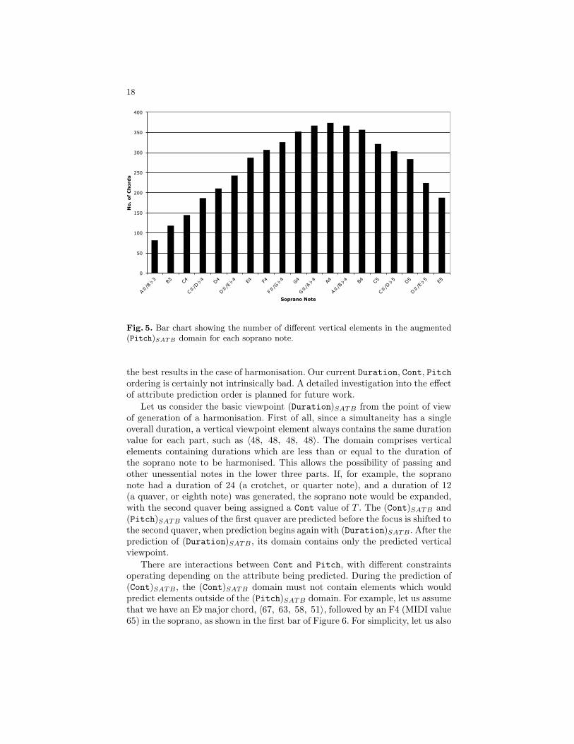
Fig. 5. Bar chart showing the number of different vertical elements in the augmented(Pitch)SATB domain for each soprano note.

the best results in the case of harmonisation. Our current Duration, Cont, Pitchordering is certainly not intrinsically bad. A detailed investigation into the effectof attribute prediction order is planned for future work.

Let us consider the basic viewpoint (Duration)SATB from the point of viewof generation of a harmonisation. First of all, since a simultaneity has a singleoverall duration, a vertical viewpoint element always contains the same durationvalue for each part, such as 〈48, 48, 48, 48〉. The domain comprises verticalelements containing durations which are less than or equal to the duration ofthe soprano note to be harmonised. This allows the possibility of passing andother unessential notes in the lower three parts. If, for example, the sopranonote had a duration of 24 (a crotchet, or quarter note), and a duration of 12(a quaver, or eighth note) was generated, the soprano note would be expanded,with the second quaver being assigned a Cont value of T . The (Cont)SATB and(Pitch)SATB values of the first quaver are predicted before the focus is shifted tothe second quaver, when prediction begins again with (Duration)SATB. After theprediction of (Duration)SATB , its domain contains only the predicted verticalviewpoint.

There are interactions between Cont and Pitch, with different constraintsoperating depending on the attribute being predicted. During the prediction of(Cont)SATB, the (Cont)SATB domain must not contain elements which wouldpredict elements outside of the (Pitch)SATB domain. For example, let us assumethat we have an E♭major chord, 〈67, 63, 58, 51〉, followed by an F4 (MIDI value65) in the soprano, as shown in the first bar of Figure 6. For simplicity, let us also

19

Fig. 6. The effect of viewpoint (Cont)SATB on a chord progression. Bar 1 shows thesoprano note to be harmonised and the preceding chord. Bars 2 to 5 illustrate theeffect of vertical (Cont)SATB elements 〈F, F, F, F 〉, 〈F, T, F, F 〉, 〈F, F, T, F 〉 and〈F, T, T, F 〉 respectively on the chosen second chord.

assume that the only vertical element in the (Pitch)SATB domain constrainedby the soprano note is 〈65, 63, 58, 50〉. The set of vertical (Cont)SATB elementscompatible with this artificially small (Pitch)SATB domain is

{〈F, F, F, F 〉 〈F, T, F, F 〉 〈F, F, T, F 〉 〈F, T, T, F 〉}.

Any other (Cont)SATB element, such as 〈F, T, T, T 〉 or 〈F, F, F, T 〉, wouldmap onto a (Pitch)SATB element which is not in the domain. Bars 2 to 5 ofFigure 6 show the chord progression resulting from each of these (Cont)SATB

elements respectively, in conventional musical notation. Even realistically sized(Pitch)SATB domains can restrict the (Cont)SATB domain beyond what mightbe expected by constraining according to the Cont attribute of the soprano note.Once (Cont)SATB has been predicted, its domain comprises a single verticalelement, and the (Pitch)SATB domain is further constrained to vertical elementswhich are compatible with the predicted vertical (Cont)SATB element.

6.4 Construction of Derived and Linked Viewpoint Domains

Derived viewpoint domains are constructed by converting each vertical elementof the relevant basic viewpoint domain (however it is currently constrained) intoa vertical element of the derived domain. By constructing the domain in this way,we can be sure that between them, the members will be able to predict all of,and only, the members of the basic domain. As with melodic domains, after eachconversion the vertical element is added to the derived domain only if it is notalready a member (recalling that the conversion function is surjective). For ex-ample, assuming a key of A, vertical (Pitch)SATB elements 〈69, 64, 61, 57〉 and〈69, 64, 61, 45〉 both map to vertical (ScaleDegree)SATB element 〈0, 7, 4, 0〉.

As with melodic domains, for links between functionally unrelated view-points, the linked domain is the Cartesian product of the individual viewpointdomains; and for links between viewpoints capable of predicting the same ba-sic viewpoint, the informal unidirectional one-to-one correspondence betweenelements of the individual viewpoint domains means that only correspondingelements are included in the linked domain (there are also correspondences be-tween Cont and Pitch, and viewpoints derived from it, as discussed above).

20

Continuing the example in the paragraph above, for a key of A, vertical ele-ments 〈〈69, 0〉, 〈64, 7〉, 〈61, 4〉, 〈57, 0〉〉 and 〈〈69, 0〉, 〈64, 7〉, 〈61, 4〉, 〈45, 0〉〉would both appear in the (Pitch ⊗ ScaleDegree)SATB domain; but 〈〈69, 0〉,〈64, 7〉, 〈61, 4〉, 〈55, 0〉〉 would not, since in the bass part the Pitch value of55 corresponds to a G, and the ScaleDegree value of 0 corresponds to an A.

The reason that we must be able to reliably construct such domains is be-cause prediction probability distributions are completed by backing off to uni-form distributions based on these domains. The various viewpoint distributionsare converted into basic viewpoint distributions prior to combination. To facili-tate combination, the distributions are sorted into the same order. An unreliabledomain construction procedure might, for example, result in one or two predic-tions being missing from some distributions, which means that at some point asuccession of probabilities will be erroneously combined.

7 Version 2 Viewpoint Domains

7.1 Introduction to Version 2

In this version, it is hypothesised that predicting all unknown symbols in a verti-cal viewpoint element (as in version 1) at the same time is neither necessary nordesirable. It is anticipated that by dividing the overall harmonisation task intoa number of subtasks (Allan and Williams, 2005; Hild et al., 1992), each mod-elled by its own multiple viewpoint system, an increase in performance can beachieved. For example, given a soprano line, the first subtask might be to predictthe entire bass line. Since there is no supporting context in the alto and tenor lay-ers yet, inter-layer linked viewpoints such as (ScaleDegree)S⊗(ScaleDegree)Bp

are used (recall that subscript p indicates the prediction layer; that is, the layerto be predicted). Once the bass line has been predicted, it becomes a supportlayer in subsequent subtasks. This version allows us to experiment with differ-ent arrangements of subtasks. For example, having predicted the bass line, is itbetter to predict the alto and tenor lines together, or one before the other? Notethat text books on harmonisation generally advocate the completion of the bassline first, in conjunction with harmonic function symbols such as Ib for tonicin first inversion. Alto and tenor notes are then added together (see Whorleyet al. (2013) for an information theoretic investigation of this subject). Anotheralternative (not implemented) would be to predict all of the notes of a chord bythe application of a sequence of subtask models before moving on to the nextchord. As in version 1, vertical viewpoint elements are restricted to using thesame viewpoint on each layer. The difference is that not all of the layers arenow necessarily represented in a vertical viewpoint element; for example, for theprediction of bass given soprano, only the soprano and bass are represented, asshown in Figure 7.

7.2 Domains

Provided we always predict only one part at a time, and always constrain thePitch domain as much as possible, we could reasonably construct full domains

21

0 0 4 2 0 2 2 4 S0 4 0 7 9 5 ? ? B

✞

✝

☎

✆

✞

✝

☎

✆

✞

✝

☎

✆✯

Fig. 7. Incomplete harmonisation of the first phrase of hymn tune Luther’s Hymn(Nun freut euch) adapted from Vaughan Williams (1933), with a sequence of verticalScaleDegree elements (comprising soprano and bass values only) underneath. A tri-gram is shown predicting the penultimate element, in which a question mark representsthe unknown ScaleDegree value.

(i.e., without having to resort to using only combinations which occur in thecorpus and test data). Let us, for example, assume that we are predicting bassgiven soprano. The Pitch domain would comprise vertical elements containingthe given soprano pitch and each of the pitches occurring in the bass in turn,giving a total of only 23 elements. We wish, however, to retain the option ofpredicting more than one part at a time; and a domain constructed in this waywhich is capable of predicting two parts at once would require up to 460 verticalviewpoint elements. The following treatment, then, assumes the use of verticalbasic viewpoint elements seen in the corpus and test data, with the option ofaugmentation with transposed elements as described in §6.2.

To obtain basic viewpoint domains for the required combination of parts,say soprano and bass only, the corpus and test data can be traversed, with eachnew soprano/bass combination (and optionally its transpositions) being addedto the relevant domain. Although not present in the domain, transposed altoand tenor notes must still be within their part ranges. Alternatively, if a domainof vertical elements containing all four parts has already been found, this can besimilarly traversed to obtain the domain of soprano/bass elements. Constructionof derived and linked viewpoint domains is then carried out in exactly the sameway as in version 1.

8 Version 3 Viewpoint Domains

8.1 Introduction to Version 3

There are two differences between version 2 and version 3. The first is that differ-ent viewpoints on different layers can now be linked; for example, ScaleDegreein the soprano can be linked with Pitch in the bass, giving inter-layer linkedviewpoint (ScaleDegree)S⊗(Pitch)Bp. The second is that linking with supportlayers (given parts) is not compulsory; so if we are given the soprano and bass,and are predicting the alto and tenor, we can, for instance, link viewpoints from

22

7 7 0 11 0 0 ? ? A4 0 7 7 4 9 ? ? T43 47 43 50 52 48 50 43 B

☛

✡

✟

✠

☛

✡

✟

✠

☛

✡

✟

✠✯

Fig. 8. Incomplete harmonisation of the first phrase of hymn tune Luther’s Hymn(Nun freut euch) adapted from Vaughan Williams (1933), with a sequence of(ScaleDegree)Ap ⊗ (ScaleDegree)Tp ⊗ (Pitch)B elements underneath. A trigram isshown predicting the penultimate element, in which question marks represent the un-known ScaleDegree values.

the alto, tenor and bass, but not soprano, as shown in Figure 8. It should benoted, however, that even if a support layer is not represented in a linked view-point, the domain is still constrained by the given note at the prediction point ofthis layer. At present, for (relative) ease of implementation, prediction layers areassigned the same viewpoint, although support layers may have any combinationof viewpoints (c.f. version 2, where the same viewpoint appears on all layers). Arelaxation of the prediction layer restriction could conceivably result in better(but more complex) models; so we are contemplating a sub-version without thisrestriction. As usual, if at any point in the event sequence a derived viewpointis undefined, an inter-layer linked viewpoint containing that viewpoint is alsoundefined.

It is necessary to modify the viewpoint selection algorithm described in §3.6.We start with a set consisting of the basic viewpoints to be predicted, whichnow comprise prediction layers only. Assuming that we are given the sopranoand bass, and are predicting the alto and tenor, one of the viewpoints in thisinitial set is (Duration)Ap ⊗ (Duration)Tp. At each iteration, we try adding inturn viewpoints such as (ScaleDegree)Ap ⊗ (ScaleDegree)Tp; and viewpointsinvolving incremental intra- or inter-layer linkages with viewpoints already inthe set, such as (Duration⊗ ScaleDegree)Ap ⊗ (Duration⊗ ScaleDegree)Tp

or (Duration)Ap ⊗ (Duration)Tp ⊗ (ScaleDegree)B. The rest of the algorithmis the same as before.

8.2 Domain Construction Issues

Version 3 viewpoints can be much more complex than any we have seen before:especially when three parts are given and we are predicting the remaining part. Inthis case, each of the four parts could have a different viewpoint; but let us beginwith something far more simple. During prediction of bass given soprano, wemay use the viewpoint (ScaleDegree)S ⊗ (Pitch)Bp. Although the constituent

23

viewpoints are able to predict the same basic viewpoint, the fact that they areassigned to different layers means that there are no correspondences which needto be taken into account; therefore taking the Cartesian product of the individuallayer domains (as constrained by the given soprano note) is a perfectly acceptableway of constructing the inter-layer linked domain. We would not wish to do so inpractice, however, for reasons outlined above. As before, we would place elementsinto the domain which correspond to Pitch combinations found in the corpusand test data (and optionally, transpositions of these combinations).

Unfortunately, most version 3 viewpoints are not as straightforward as this.We are predicting basic viewpoints Duration, Cont and Pitch, each of whichhas its own domain of a particular size; there are other basic viewpoints whichwe assume to be given; there are many derived viewpoints, most of them derivedfrom Pitch, having domains of various sizes; and there are up to four layers rep-resented in any viewpoint. A general method for reliably constructing domainsfor these complex viewpoints is required. As usual, the domains must be ableto predict all of, and only, the members of the basic viewpoint domain(s). It ispossible for each layer to have a different viewpoint; therefore it is expedientto deal with each layer in turn. This being the case, to achieve precisely thecorrect combinations of viewpoint elements, we need to know in advance howmany elements there are in the provisional inter-layer linked viewpoint domain(which, as we shall see, may end up containing undefined or duplicate elementswhich must be removed). To calculate this number, we also need to know theset of basic viewpoints that the constituent viewpoints are derived from, that is,the type set 〈τ〉 (note that the set of basic viewpoints that the inter-layer linkedviewpoint is able to predict is a subset of 〈τ〉, since only constituent viewpointsof the prediction layers should be considered); since we can determine what thedomains of these basic viewpoints are for the combination of layers in question,we are easily able to ascertain their sizes. For the purposes of constructing aprovisional inter-layer linked domain, we assume that the size of each deriveddomain (covering all of the parts represented in the viewpoint) is the same asthat of the relevant basic domain. This means that we can relatively easily assigninner- and outer-multipliers to each basic or derived constituent viewpoint priorto construction of the inter-layer linked viewpoint. These multipliers respectivelydetermine the number of times a primitive domain element is repeated prior tomoving on to the next, and the number of times the entire primitive domain isrepeated (along with any internal repeats).

As a simple example, let us assume that there are only two elements (A andB) in the primitive domain, and that the inner- and outer-multipliers have valuesof 3 and 2 respectively. Figure 9 illustrates the effect of the multipliers on theprimitive domain. The elements of this domain are each shown as the root ofa tree. The outer-multiplier is 2; therefore each root divides into two branches,resulting in the primitive domain being shown twice. The inner-multiplier is 3; soeach of the four nodes splits into three, thereby duplicating elements within eachof the copies of the primitive domain. The number of elements in the provisional

24

A A A B B B A A A B B B

A B A B

A B❳❳❳❳❳❳❳❳❳❳❳❳❳❳❳❳

❳❳❳❳❳❳❳❳❳❳❳❳❳❳❳❳

✡✡

✡✡✡

❏❏❏❏❏

✡✡

✡✡✡

❏❏❏❏❏

✡✡

✡✡✡

❏❏❏❏❏

✡✡

✡✡✡

❏❏❏❏❏

Fig. 9. Trees illustrating the effect of multipliers on primitive domain {A,B}. Branch-ing from the roots is due to the outer-multiplier (2); and further branching to producethe leaves is due to the inner-multiplier (3).

inter-layer linked domain is the same as the total number of leaves on the trees,which is the product of the primitive domain size and the two multipliers.

8.3 Determination of Multipliers

In calculating the multipliers, we assume that the basic viewpoints are in aparticular order: Duration, Cont, Pitch, followed by other basic viewpoints.The order of the other basic viewpoints is not important, as in our research theyare given and therefore effectively have a domain containing only one element.Once we know which of Duration, Cont and Pitch the constituent viewpointsare derived from, we can assign multipliers according to their relative positions inthe ordered list. For a particular basic viewpoint, the inner- and outer-multipliersare the product of the domain sizes of any basic viewpoints occurring after it,and before it, respectively. The default value of both is 1. For example, considera linked viewpoint with constituents derived from Duration, Cont and Pitch,and which also contains viewpoint LastInPhrase (derived from basic viewpointPhrase). If we assume that Duration, Cont and Pitch have domain sizes of5, 10 and 40 respectively, then for any constituent viewpoint able to predictDuration, the inner- and outer-multipliers are 400 and 1; for any constituentviewpoint able to predict Cont, the inner- and outer-multipliers are 40 and 5; forany constituent viewpoint able to predict Pitch, the inner- and outer-multipliersare 1 and 50; and for any other constituent viewpoint (e.g., LastInPhrase), theinner- and outer-multipliers are 1 and 2000 respectively. Generalised algorithmsfor the determination of multipliers can be found in Algorithms 1, 2 and 3in Appendix A, along with a line-by-line description of their use in the aboveexample.

8.4 Domain Construction Procedure

This procedure will be illustrated by a modified real example: only a small subsetof the actual Pitch domain is used, comprising note names such as A♭4 rather

25

than MIDI numbers, in order to make the illustration more readily intelligible.We are predicting bass given soprano using, amongst other viewpoints,

(Duration⊗ Pitch)S ⊗ (Cont⊗ ScaleDegree)Bp.

The set of basic viewpoints (type set 〈τ〉) that the above’s constituent viewpointsare derived from is {Duration, Cont, Pitch}. The Duration attribute of a bassnote has already been predicted; therefore the Duration domain contains onlyone element:

{〈〈S, 0, Duration, 〈24〉〉 〈B, 0, Duration, 〈24〉〉〉}.

The next attribute to be predicted is Cont. The given soprano note has a Cont

attribute of F ; therefore the domain is constrained to two elements:

{〈〈S, 0, Cont, 〈F 〉〉 〈B, 0, Cont, 〈T 〉〉〉,

〈〈S, 0, Cont, 〈F 〉〉 〈B, 0, Cont, 〈F 〉〉〉}.

The 5-element Pitch domain (constrained to have a soprano A♭4) is

{〈〈S, 0, Pitch, 〈A♭4〉〉 〈B, 0, Pitch, 〈F2〉〉〉,

〈〈S, 0, Pitch, 〈A♭4〉〉 〈B, 0, Pitch, 〈E♭3〉〉〉,〈〈S, 0, Pitch, 〈A♭4〉〉 〈B, 0, Pitch, 〈E3〉〉〉,〈〈S, 0, Pitch, 〈A♭4〉〉 〈B, 0, Pitch, 〈F3〉〉〉,〈〈S, 0, Pitch, 〈A♭4〉〉 〈B, 0, Pitch, 〈F♯3〉〉〉}.

The highest part (in terms of pitch) is dealt with first. If the viewpointon this layer is, or contains, a basic viewpoint, each of the symbols or valuesbelonging to that layer in the basic viewpoint domain is added, in turn, to whatwill become the inter-layer linked viewpoint domain, with repeats determinedby the inner- and outer-multipliers. If the viewpoint is derived, the procedureis the same except that each basic viewpoint symbol is converted to a derivedviewpoint symbol. In the example, viewpoint Duration in the soprano part isdealt with first. Its inner-multiplier is the product of the Cont and Pitch domainsizes, which is 10, and its outer-multiplier is 1. The provisional linked domaintherefore starts off as

{〈〈S, 0, Duration, 〈24〉〉〉, 〈〈S, 0, Duration, 〈24〉〉〉,〈〈S, 0, Duration, 〈24〉〉〉, 〈〈S, 0, Duration, 〈24〉〉〉,〈〈S, 0, Duration, 〈24〉〉〉, 〈〈S, 0, Duration, 〈24〉〉〉,〈〈S, 0, Duration, 〈24〉〉〉, 〈〈S, 0, Duration, 〈24〉〉〉,〈〈S, 0, Duration, 〈24〉〉〉, 〈〈S, 0, Duration, 〈24〉〉〉}.

At this point, the provisional inter-layer linked viewpoint domain contains allof the elements we need (and probably more), albeit that they are incomplete.If there is a second basic or derived viewpoint associated with this layer (i.e.,a constituent of an intra-layer linked viewpoint), then the same procedure isfollowed except that the symbols are linked with the symbols already in theprovisional domain, in the same order as the original additions to the domain.

26

In the example, viewpoint Pitch in the soprano part is dealt with next. Itsinner-multiplier is 1, and its outer-multiplier is the product of the Duration andCont domain sizes, which is 2. The provisional linked domain then becomes

{〈〈S, 0, Duration⊗ Pitch, 〈24, A♭4〉〉〉,

〈〈S, 0, Duration⊗ Pitch, 〈24, A♭4〉〉〉,

〈〈S, 0, Duration⊗ Pitch, 〈24, A♭4〉〉〉,

〈〈S, 0, Duration⊗ Pitch, 〈24, A♭4〉〉〉,

〈〈S, 0, Duration⊗ Pitch, 〈24, A♭4〉〉〉,

〈〈S, 0, Duration⊗ Pitch, 〈24, A♭4〉〉〉,

〈〈S, 0, Duration⊗ Pitch, 〈24, A♭4〉〉〉,

〈〈S, 0, Duration⊗ Pitch, 〈24, A♭4〉〉〉,

〈〈S, 0, Duration⊗ Pitch, 〈24, A♭4〉〉〉,

〈〈S, 0, Duration⊗ Pitch, 〈24, A♭4〉〉〉}.

We then move on to the next layer, again adding to the elements alreadyin the provisional domain, and so on, until all the layers have been dealt with.There is only one other layer in the example, the bass part, which contains theintra-layer linked viewpoint Cont ⊗ ScaleDegree. Primitive viewpoint Cont isdealt with first; its inner-multiplier is 5 (the size of the Pitch domain), and itsouter-multiplier is 1 (the size of the Duration domain). The provisional linkeddomain then becomes

{〈〈S, 0, Duration⊗ Pitch, 〈24, A♭4〉〉, 〈B, 0, Cont, 〈T 〉〉〉,

〈〈S, 0, Duration⊗ Pitch, 〈24, A♭4〉〉, 〈B, 0, Cont, 〈T 〉〉〉,

〈〈S, 0, Duration⊗ Pitch, 〈24, A♭4〉〉, 〈B, 0, Cont, 〈T 〉〉〉,

〈〈S, 0, Duration⊗ Pitch, 〈24, A♭4〉〉, 〈B, 0, Cont, 〈T 〉〉〉,

〈〈S, 0, Duration⊗ Pitch, 〈24, A♭4〉〉, 〈B, 0, Cont, 〈T 〉〉〉,

〈〈S, 0, Duration⊗ Pitch, 〈24, A♭4〉〉, 〈B, 0, Cont, 〈F 〉〉〉,

〈〈S, 0, Duration⊗ Pitch, 〈24, A♭4〉〉, 〈B, 0, Cont, 〈F 〉〉〉,

〈〈S, 0, Duration⊗ Pitch, 〈24, A♭4〉〉, 〈B, 0, Cont, 〈F 〉〉〉,

〈〈S, 0, Duration⊗ Pitch, 〈24, A♭4〉〉, 〈B, 0, Cont, 〈F 〉〉〉,

〈〈S, 0, Duration⊗ Pitch, 〈24, A♭4〉〉, 〈B, 0, Cont, 〈F 〉〉〉}.

The final viewpoint to be added is ScaleDegree in the bass part; becauseit predicts Pitch, its inner-multiplier is 1, and its outer-multiplier is 2. Thereis a particular problem to be overcome with respect to the intra-layer linkingof Cont with Pitch, or viewpoints derived from it, however. As we have seenin §6.3, there is an interaction between the Cont and Pitch domains; thereforethe Cartesian product would contain pairings making no logical sense. In thiscase, as the Pitch domain is traversed, the Pitch symbol is checked against therelevant Cont symbol (which is already in the provisional domain): if the pairingmakes logical sense, the Pitch symbol, or a symbol derived from it, is added tothe element in the provisional domain as usual; if not, the element is tagged asundefined. The previous note was F3 (MIDI value 53); therefore 53 is the onlyPitch value which can be sensibly paired with a Cont value of T . The tonic is

27

E♭; therefore F has a ScaleDegree value of 2. The provisional linked domainthen becomes

{〈〈S, 0, Duration⊗ Pitch, 〈24, A♭4〉〉, undef 〉,

〈〈S, 0, Duration⊗ Pitch, 〈24, A♭4〉〉, undef 〉,

〈〈S, 0, Duration⊗ Pitch, 〈24, A♭4〉〉, undef 〉,

〈〈S, 0, Duration⊗ Pitch, 〈24, A♭4〉〉, 〈B, 0, Cont⊗ ScaleDegree, 〈T, 2〉〉〉,

〈〈S, 0, Duration⊗ Pitch, 〈24, A♭4〉〉, undef 〉,

〈〈S, 0, Duration⊗ Pitch, 〈24, A♭4〉〉, 〈B, 0, Cont⊗ ScaleDegree, 〈F, 2〉〉〉,

〈〈S, 0, Duration⊗ Pitch, 〈24, A♭4〉〉, 〈B, 0, Cont⊗ ScaleDegree, 〈F, 0〉〉〉,

〈〈S, 0, Duration⊗ Pitch, 〈24, A♭4〉〉, 〈B, 0, Cont⊗ ScaleDegree, 〈F, 1〉〉〉,

〈〈S, 0, Duration⊗ Pitch, 〈24, A♭4〉〉, 〈B, 0, Cont⊗ ScaleDegree, 〈F, 2〉〉〉,

〈〈S, 0, Duration⊗ Pitch, 〈24, A♭4〉〉, 〈B, 0, Cont⊗ ScaleDegree, 〈F, 3〉〉〉}.

The provisional domain, constructed in this way in order to ensure thatsymbols which do not correspond with each other are not linked, may containelements tagged as undefined, and may also contain duplicate elements; thereforethe final inter-layer linked viewpoint domain is achieved once undefined andduplicate elements have been removed:

{〈〈S, 0, Duration⊗ Pitch, 〈24, A♭4〉〉, 〈B, 0, Cont⊗ ScaleDegree, 〈T, 2〉〉〉,

〈〈S, 0, Duration⊗ Pitch, 〈24, A♭4〉〉, 〈B, 0, Cont⊗ ScaleDegree, 〈F, 0〉〉〉,

〈〈S, 0, Duration⊗ Pitch, 〈24, A♭4〉〉, 〈B, 0, Cont⊗ ScaleDegree, 〈F, 1〉〉〉,

〈〈S, 0, Duration⊗ Pitch, 〈24, A♭4〉〉, 〈B, 0, Cont⊗ ScaleDegree, 〈F, 2〉〉〉,

〈〈S, 0, Duration⊗ Pitch, 〈24, A♭4〉〉, 〈B, 0, Cont⊗ ScaleDegree, 〈F, 3〉〉〉}.

A generalised algorithm for the construction of version 3 inter-layer linkedviewpoint domains can be found in Algorithm 4 in Appendix A, along with aline-by-line description of its use in the above example.

9 Time Complexity Analysis

To demonstrate the utility of reducing domain size, we have carried out an empir-ical time complexity analysis on version 1 prediction runs. This involved runningthe computer model with different numbers of viewpoints, different sizes of cor-pus, and different types of (Pitch)SATB domain (seen, augmented and full).Maximum N-gram order also influences run time, but we have not yet investi-gated it; all runs used a maximum N-gram order of 3. Seen (Duration)SATB

and (Cont)SATB domains are used throughout, which are small enough to beneglected for the purposes of this analysis. During the course of this exercise,we have also determined how (Pitch)SATB domain size varies with corpus/testdata size for the seen, augmented and full domain cases. It is with this that weshall begin.

28

0

200

400

600

800

1000

1200

1400

0 1000 2000 3000 4000 5000 6000

No. Events in Corpus/Test Data

Seen

(Pitch

)SATB D

om

ain

Siz

e

Fig. 10. Plot of number of events in the corpus/test data against seen (Pitch)SATB

domain size.

9.1 Variation of Domain Size with Corpus/Test Data Size

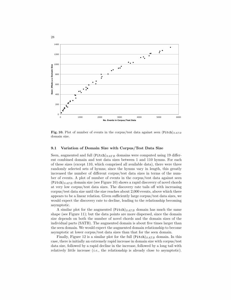
Seen, augmented and full (Pitch)SATB domains were computed using 19 differ-ent combined domain and test data sizes between 1 and 110 hymns. For eachof these sizes (except 110, which comprised all available data), there were threerandomly selected sets of hymns; since the hymns vary in length, this greatlyincreased the number of different corpus/test data sizes in terms of the num-ber of events. A plot of number of events in the corpus/test data against seen(Pitch)SATB domain size (see Figure 10) shows a rapid discovery of novel chordsat very low corpus/test data sizes. The discovery rate tails off with increasingcorpus/test data size until the size reaches about 2,000 events, above which thereappears to be a linear relation. Given sufficiently large corpus/test data sizes, wewould expect the discovery rate to decline, leading to the relationship becomingasymptotic.

A similar plot for the augmented (Pitch)SATB domain has much the sameshape (see Figure 11); but the data points are more dispersed, since the domainsize depends on both the number of novel chords and the domain sizes of theindividual parts (SATB). The augmented domain is about five times larger thanthe seen domain. We would expect the augmented domain relationship to becomeasymptotic at lower corpus/test data sizes than that for the seen domain.

Finally, Figure 12 is a similar plot for the full (Pitch)SATB domain. In thiscase, there is initially an extremely rapid increase in domain size with corpus/testdata size, followed by a rapid decline in the increase, followed by a long tail withrelatively little increase (i.e., the relationship is already close to asymptotic).

29

0

1000

2000

3000

4000

5000

6000

7000

8000

0 1000 2000 3000 4000 5000 6000

No. Events in Corpus/Test Data

Au

gm

en

ted (Pitch

)SATB D

om

ain

Siz

e

Fig. 11. Plot of number of events in the corpus/test data against augmented(Pitch)SATB domain size.

The data points are very dispersed, due to the fact that domain size dependssolely on the domain sizes of the individual parts. A log curve seems to fit thisdata best, which is not the case for the seen and augmented data.

9.2 Effect of Domain Size on Program Running Time

Figure 13 is a log-log plot of (Pitch)SATB domain size against time for thelearning phase of the program, which was run using a corpus of 30 hymns andmultiple viewpoint systems comprising 2 and 10 viewpoints. There are threedomain sizes, corresponding to the seen, augmented and full domains. The seendomain causes the program to run about two orders of magnitude faster thanthe full domain. Encouragingly, the use of the augmented domain results in arunning time which is not too much slower than that of the seen domain.

For the prediction phase of the program (Duration, Cont and Pitch predic-tion), the relative differences in running time are even greater: the seen domaincauses the program to run about three orders of magnitude faster than the fulldomain (see Figure 14). The running time of the program using the augmenteddomain is still fairly close to that using the seen domain.

We have demonstrated the utility of reducing the (Pitch)SATB domain size.The full (Pitch)SATB domain causes the program to run very slowly even for theprediction of only one short harmonisation. For viewpoint selection runs, whichinvolve ten-fold cross-validation of the corpus, the situation is far worse. Duringthe course of such a run, many multiple viewpoint systems are tried. For each of

30

0

20000

40000

60000

80000

100000

120000

140000

160000

180000

0 1000 2000 3000 4000 5000 6000

No. Events in Corpus/Test Data

Fu

ll (Pitch

)SATB D

om

ain

Siz

e

Fig. 12. Plot of number of events in the corpus/test data against full (Pitch)SATB

domain size.

0.1

1

10

100

1000

100 1000 10000 100000 1000000

(Pitch)SATB Domain Size

Tim

e/

s

2 viewpoints

10 viewpoints

Fig. 13. Log-log plot of (Pitch)SATB domain size against time for the learning phaseof the program, which was run using a corpus of 30 hymns and multiple viewpointsystems comprising 2 and 10 viewpoints.

31

0.1

1

10

100

1000

100 1000 10000 100000 1000000

(Pitch)SATB Domain Size

Tim

e/

s

2 viewpoints

10 viewpoints

Fig. 14. Log-log plot of (Pitch)SATB domain size against time for the prediction phaseof the program, which was run using a corpus of 30 hymns and multiple viewpointsystems comprising 2 and 10 viewpoints. A single hymn tune harmonisation comprising33 events was predicted.

these systems, the learning phase is run ten times, and every harmonisation inthe corpus is predicted. Since it is clearly not practical to use the full domain,further analysis will concentrate on the use of the seen and augmented domains.Time complexities will be derived in terms of number of viewpoints, size ofcorpus and size of test data, to give prospective developers of similar programsan idea of their effect on running time.

9.3 Empirical Time Complexity Analysis Using Seen andAugmented Domains

In this more detailed analysis, the learning phase is split into domain construc-tion and model construction phases. First of all, it is appropriate to explain whywe have decided to derive time complexities empirically rather than analytically.The domain construction phase should be the easiest to analyse, since the num-ber of viewpoints is irrelevant: we are only constructing the three basic domainsduring this phase. We can simplify things further by neglecting the Duration

and Cont domains, which are very small in comparison with that of Pitch. Theprocedure is to traverse the corpus and test data, adding previously unseen el-ements to the Pitch domain. The traversal time, ignoring domain processingtime, is proportional to the number of events in the corpus and test data; butwe cannot ignore domain processing. For each event in the corpus and test data,

32

its Pitch element must, in the worst case, be compared with every element inthe Pitch domain, which increases in size throughout this process. The rate ofincrease and ultimate size is much greater for the augmented domain than forthe seen domain. In neither case, however, can this information be accuratelydetermined a priori for any given corpus and test data (although inspection ofFigures 10 and 11 can give a rough idea for this style of music); we consider itbetter, therefore, to derive the time complexity empirically.

Having said that, we know that in this particular case there are only 882elements in the seen domain, compared with 2,601 events in the corpus andtest data (a ratio of 0.34). If we define nc to be the number of events in thecorpus and ntd to be the number of events in the test data, at worst the timecomplexity for the seen domain is O((nc + ntd)

1.34). On the other hand, thereare 5,040 elements in the augmented domain; therefore in this case we wouldexpect a complexity of O((nc + ntd)

2.94) at worst.

Since time complexities for the model construction and prediction phases areeven more difficult to derive analytically (e.g., we cannot determine the size andstructure of the viewpoint models a priori), we have made no attempt to do so.Let us now look at the empirical analyses.

Domain Construction Phase Figure 15 shows a plot of number of viewpointsagainst time for the seen domain construction phase of the program, which wasrun using corpora of 5, 10, 15, 20, 25 and 30 hymns. Each data point has amean time of ten runs, each run using a different randomly selected multipleviewpoint system capable of predicting Duration, Cont and Pitch (the ten runsvary widely in duration). Straight lines fit the data reasonably well. All six linesare close to horizontal; therefore it has been concluded that, in reality, the runtimes are constant with respect to the number of viewpoints. This makes sense,considering that only the three basic viewpoint domains are constructed duringthis phase. A similar plot for the augmented domain (see Figure 16) also leadsus to the conclusion that the times are constant with respect to the number ofviewpoints. The times are taken to be those in the centre of the fitted lines;that is, at the 6 viewpoint mark. Two other data sets were also generated andanalysed, using different sets of hymns for each corpus size (resulting in differentnumbers of corpus events). The graphs, which are not shown here, are similarto those for the first data set.

Bearing in mind that the test data (in addition to the corpus) is taken intoaccount when constructing domains, we are now in a position to plot the numberof events in the corpus and test data against time; see Figure 17, which makesuse of all three of the generated data sets. The data is rather sparse and scat-tered; but a straight line seems to produce a reasonable fit for the seen domain,and a quadratic curve a reasonable fit for the augmented domain (both fits areconstrained to extend to the origin). The fact that time increases more rapidlywith increasing number of events for the augmented domain is not unreasonable,since there is additional processing involved in its construction.

33

y = -0.0032x + 0.1356

y = -0.002x + 0.2509

y = 0.0014x + 0.3193

y = -0.0079x + 0.5681

y = -0.0076x + 0.5602

y = -0.0035x + 0.6785

0

0.1

0.2

0.3

0.4

0.5

0.6

0.7

2 3 4 5 6 7 8 9 10

No. Viewpoints

Tim

e/

s

5

10

15

20

25

30

Linear(5)

Linear(10)Linear(15)Linear(20)

Linear(25)Linear(30)

Fig. 15. Plot of number of viewpoints against time for the seen domain constructionphase of the program, which was run using corpora of 5, 10, 15, 20, 25 and 30 hymns.

y = 0.0017x + 0.108

y = 0.0021x + 0.237

y = 0.0045x + 0.317

y = 0.018x + 0.4995

y = 0.0023x + 0.6261

y = -0.0026x + 0.8388

0

0.1

0.2

0.3

0.4

0.5

0.6

0.7

0.8

0.9

2 3 4 5 6 7 8 9 10

No. Viewpoints

Tim

e/

s

5

10

15

20

25

30

Linear(5)

Linear(10)

Linear(15)

Linear(20)

Linear(25)

Linear(30)

Fig. 16. Plot of number of viewpoints against time for the augmented domain con-struction phase of the program, which was run using corpora of 5, 10, 15, 20, 25 and30 hymns.

34

y = 0.0004x

y = 1E-07x2 + 0.0004x

0

0.1

0.2

0.3

0.4

0.5

0.6

0.7

0.8

0.9

0 200 400 600 800 1000 1200 1400 1600

No. Events in Corpus and Test Data

Tim

e/

s

seen

aug

Linear(seen)

Poly.(aug)

Fig. 17. Plot of number of events in the corpus and test data against time for the seenand augmented domain construction phases of the program.

From the foregoing we gather that the time complexity of the domain con-struction phase of the program is at worst O((nc + ntd)

2). In other words, run

time is proportional to the square of the number of events in the corpus and testdata. This is better than the semi-analytically derived worst case complexity ofO((nc + ntd)

2.94), which necessarily made use of simplifying assumptions.

Model Construction Phase Figure 18 shows a plot of number of viewpointsagainst time for the model construction phase of the program, which was runusing the seen (Pitch)SATB domain and corpora of 5, 10, 15, 20, 25 and 30hymns. Again, straight lines fit the data reasonably well; but in this case thereis a definite increase in run time with increasing number of viewpoints, whichis due to the fact that a separate model needs to be built for each viewpoint.A similar plot for the augmented (Pitch)SATB domain (see Figure 19) shows alarger increase in run time with increasing number of viewpoints. This is almostcertainly not due to an increase in the time required to construct the modelsfrom the corpus per se, but rather to the time needed for other processing in-volving domains in this part of the program. Again, two other data sets werealso generated and analysed, with similar results.

We can now plot the number of of events in the corpus against time; seeFigure 20. The times are taken from the fitted lines on the plots described aboverather than from the original data points. In this case, the best fit to the datais a quadratic curve (constrained to extend to the origin); but the trend is closeto linear for the range of data analysed. As expected, run time increases withthe number of events in the corpus: there is a more rapid increase in time with

35

y = 0.0055x + 0.0289

y = 0.0113x + 0.0682

y = 0.0221x + 0.1044

y = 0.0333x + 0.154

y = 0.0425x + 0.2194

y = 0.0553x + 0.2474

0

0.1

0.2

0.3

0.4

0.5

0.6

0.7

0.8

0.9

2 3 4 5 6 7 8 9 10

No. Viewpoints

Tim

e/

s

5

10

15

20

25

30

Linear(5)Linear(10)Linear(15)Linear(20)Linear(25)Linear(30)

Fig. 18. Plot of number of viewpoints against time for the model construction phaseof the program, which was run using the seen (Pitch)SATB domain and corpora of 5,10, 15, 20, 25 and 30 hymns.

y = 0.0187x + 0.0209

y = 0.0398x + 0.0877

y = 0.0702x + 0.1165

y = 0.0887x + 0.239

y = 0.1293x + 0.2173

y = 0.1516x + 0.2384

0

0.2

0.4

0.6

0.8

1

1.2

1.4

1.6

1.8

2

2 3 4 5 6 7 8 9 10

No. Viewpoints

Tim

e/

s

5

10

15

20

25

30

Linear(5)

Linear(10)

Linear(15)Linear(20)

Linear(25)

Linear(30)

Fig. 19. Plot of number of viewpoints against time for the model construction phaseof the program, which was run using the augmented (Pitch)SATB domain and corporaof 5, 10, 15, 20, 25 and 30 hymns.

36

y = 7E-08x2 + 0.0001x

y = 2E-07x2 + 0.0003x

y = 7E-08x2 + 0.0003x

y = 2E-07x2 + 0.0009x

0

0.2

0.4

0.6

0.8

1

1.2

1.4

1.6

1.8

0 200 400 600 800 1000 1200 1400 1600

No. Events in Corpus

Tim

e/

s

seen 2 viewpoints

seen 10 viewpoints

aug 2 viewpoints

aug 10 viewpoints

Poly. (seen 2 viewpoints)

Poly. (seen 10 viewpoints)

Poly. (aug 2 viewpoints)

Poly. (aug 10 viewpoints)

Fig. 20. Plot of number of events in the corpus against time for the model constructionphase of the program, using seen and augmented (Pitch)SATB domains and multipleviewpoint system sizes of 2 and 10 viewpoints.

increasing number of viewpoints, and the augmented domain gives rise to longerrun times than the seen domain.

If we define v to be the number of viewpoints, then from the above we con-clude that the time complexity of the model construction phase of the programis O(vn2

c). In other words, run time is proportional to the number of viewpoints,and also proportional to the square of the number of events in the corpus. For therange of data analysed here, however, we can say that run time is approximatelyproportional to nc.

Prediction Phase Figure 21 shows a plot of number of viewpoints againsttime for the prediction phase of the program, which was run using the seen(Pitch)SATB domain and corpora of 5, 10, 15, 20, 25 and 30 hymns. Once more,there is a reasonably good linear fit to the data, with increasing run time resultingfrom increasing number of viewpoints. The reason for this is that more predictionprobability distributions need to be constructed and combined as the numberof viewpoints increases. A similar plot for the augmented (Pitch)SATB domain(see Figure 22) shows a larger increase in run time with increasing number ofviewpoints. Once more, two other data sets were also generated and analysed,with similar results.

Figure 23 shows a plot of the number of events in the the corpus againsttime (taken from the fitted lines on the plots described above). The data is bestfitted using straight lines, which have been constrained to extend to the origin.Again, run time increases with the number of events in the corpus, and the

37

y = 0.01x + 0.0262

y = 0.0232x + 0.0554

y = 0.0277x + 0.0799

y = 0.0467x + 0.0831

y = 0.0526x + 0.1136

y = 0.0519x + 0.1668

0

0.1

0.2

0.3

0.4

0.5

0.6

0.7

0.8

2 3 4 5 6 7 8 9 10

No. Viewpoints

Tim

e/

s

5

10

15

20

25

30

Linear(5)Linear(10)Linear(15)Linear(20)Linear(25)Linear(30)

Fig. 21. Plot of number of viewpoints against time for the prediction phase of theprogram, which was run using the seen (Pitch)SATB domain and corpora of 5, 10, 15,20, 25 and 30 hymns.

y = 0.0378x + 0.116

y = 0.0883x + 0.1977

y = 0.118x + 0.3314

y = 0.1641x + 0.3748

y = 0.2232x + 0.407

y = 0.2343x + 0.4969

0

0.5

1

1.5

2

2.5

3

2 3 4 5 6 7 8 9 10

No. Viewpoints

Tim

e/

s

5

10

15

20

25

30

Linear(5)Linear(10)Linear(15)Linear(20)Linear(25)Linear(30)

Fig. 22. Plot of number of viewpoints against time for the prediction phase of theprogram, which was run using the augmented (Pitch)SATB domain and corpora of 5,10, 15, 20, 25 and 30 hymns.

38

y = 0.0002x

y = 0.0005x

y = 0.0007x

y = 0.002x

0

0.5

1

1.5

2

2.5

3

0 200 400 600 800 1000 1200 1400 1600

No. Events in Corpus

Tim

e/

s

seen 2 viewpoints

seen 10 viewpoints

aug 2 viewpoints

aug 10 viewpoints

Linear (seen 2 viewpoints)

Linear (seen 10 viewpoints)

Linear (aug 2 viewpoints)

Linear (aug 10 viewpoints)

Fig. 23. Plot of number of events in the corpus against time for the prediction phase ofthe program, using seen and augmented (Pitch)SATB domains and multiple viewpointsystem sizes of 2 and 10 viewpoints.

effect of domain type and number of viewpoints is similar to that in the modelconstruction phase.

We can be fairly certain, without doing experiments, that the run time ofthis phase is proportional to the number of events in the test data being pre-dicted. This, combined with the above analysis, results in a time complexity ofO(vncntd) for the prediction phase of the program. In other words, run time isproportional to the number of viewpoints, the size of the corpus, and the size ofthe test data.

Complete Prediction Run The time complexity of a complete predictionrun is the same as the worst complexity of the three constituent phases, whichis O(vn2

c) as for model construction.

9.4 Time complexity Analysis of Viewpoint Selection

For viewpoint selection, an important factor in determining run time is the num-ber of primitive viewpoints vp in a pool to be used in the stepwise optimisationof the multiple viewpoint system. At any viewpoint addition stage, single ad-ditions are made to the current multiple viewpoint system, and each of thesenew systems is evaluated using ten-fold cross-validation. In the limiting case,each primitive viewpoint in turn is added to the current system on its own andas part of a link with primitive viewpoints already in the system. This meansthat an evaluation is run the same number of times (at most) for each primitive

39

viewpoint in the pool, which in turn means that run time is proportional to vp(with a very large coefficient). This is only approximately true, however, sincethe optimisation path can change dramatically with the addition of a primitiveviewpoint to the pool; it could, for example, result in a different number of view-point addition stages, which cannot be predicted in advance. With this provisoin mind, the time complexity of a viewpoint selection run is O(vpvn

2c), where v is

the number of viewpoints in the ultimately selected multiple viewpoint system.

9.5 Time Complexity of Versions 2 and 3

Although no analysis has yet been done of the time complexity of versions 2and 3, we anticipate that it will be broadly the same as for version 1 except forthe additional factor of prediction in stages. If, for example, the alto, tenor andbass parts are predicted one after the other, the version 2 run time is likely tobe approximately three times that for prediction of ATB together. For version3, each each successive prediction stage will take longer than the preceding one.Other than that, coefficients and constants are likely to be higher in versions 2and 3 (especially 3), thereby contributing to longer run times.

10 Harmony Produced by Our Best Model to Date

Although the focus of this article is the alleviation of time complexity, and inparticular its consequences for the reliable and efficient construction of domains,we have included four automatically generated hymn tune harmonisations togive a flavour of what the multiple viewpoint models can do. They were deliber-ately chosen to demonstrate a range of quality. All of these harmonisations weregenerated using the lowest cross-entropy model found so far, which is a version3 long- and short-term model using the augmented Pitch domain generating Bgiven S followed by AT given SB. Although a fifty-hymn corpus was used duringviewpoint selection (for time complexity reasons), generation was undertakenusing a hundred-hymn corpus.

Before looking at the harmonisations, we need to explain the concept of prob-ability thresholds. The generation of harmony relies on the random sampling ofprediction probability distributions. It was quickly very obvious to us, judgingby the quality (or rather, the lack of it) of generated harmonisations, that a mod-ification to the generation procedure would be required to produce reasonablygood harmony. The problem was that random sampling sometimes generated achord of very low probability, which was bad in itself because it was likely tobe inappropriate in its context; but also bad because it then formed part of thenext chord’s context, which had probably rarely or never been seen in the cor-pus. This led to the generation of more low probability chords. The solution weproposed was to disallow the use of predictions below a chosen value, the prob-ability threshold, defined as a fraction of the highest prediction probability in agiven distribution. This definition ensures that there is always at least one usableprediction in the distribution, however high the threshold. Bearing in mind that

40

an expert musician faced with the task of harmonising a melody would consideronly a limited number of the more likely options for each chord position, weconsidered the removal of low probability predictions to be a reasonable solutionto the problem (unfortunately, low probability predictions known to be accept-able are disallowed along with those known to be unacceptable; better solutionswill be sought in future work). The following harmonisations were all generatedusing (Dur)SB, (Dur)SATB, (Cont)SB and (Cont)SATB probability thresholds of0.5; a (Pitch)SB threshold of 0.2; and a (Pitch)SATB threshold of 0.4.

A harmonisation of hymn tune Bromsgrove (Vaughan Williams 1933, hymnno. 144) is shown in Figure 24. Let us first examine what is wrong with this leastsuccessful of the four harmonisations. There are four parallel octaves within thefirst three bars, and another straddling bars 8 and 9. The change of harmony istoo rapid in the first half of the second bar. There are unnecessary repeated notesin bars 5, 6, 7, 14 and 17; and the last chords of bars 13 and 16 are discordant.On the third beat of bar 5 the alto and tenor notes could be better chosen tomake smoother chord progressions. In bar 11 there is a plagal cadence in thekey of F major with an incorrect strong-to-weak metrical arrangement; and thepiece does not end on a recognisable cadence. Although the harmony is generallyweak, there are some good points. The modulation to the relative minor in thefirst phrase is interesting, although the appearance of an F♯ would have made itmore convincing. The modulation to F major in the second phrase is reasonablywell executed, ending with a solid ii7b–V–I.

Figure 25 shows a slightly more successful harmonisation of hymn tune Dasist meine Freude (Vaughan Williams 1933, hymn no. 97). Although the harmonysounds more convincing, there is still plenty wrong with it. There is a parallelfifth in bar 12 and a parallel octave in bar 13 (both between tenor and bass).Similarly, there is a parallel unison straddling bars 5 and 6. There are unnecessaryrepeated notes in bars 4, 5, 8 and 12; and the last chord of bar 9 is discordant.There are unessential notes which are not properly resolved in bars 1 and 11.The soprano note on the first beat of bar 2 is below the preceding alto note;that is, the parts overlap, which is frowned upon. There is similar overlappingbetween tenor and bass in bars 7, 8, 9 and 11. The last chord of bar 13 (ignoringthe auxiliary note) fulfils some of the criteria for a passing 6

4, in that it is a

metrically weak Ic approached by step; importantly, however, it is not quittedby step. There is not a proper cadence at the end of bar 6, and the final cadenceis weak. On the other hand, most others are strong perfect cadences, with animperfect cadence occurring at the end of bar 10. The ii7b–I (in C major) atthe end of bar 8 has the flavour of a plagal cadence, since the first chord canbe heard as a subdominant chord with an added sixth. A well executed passingnote at the end of bar 3 goes some way to disguising a parallel octave and a falserelation. The use of modulation makes the harmony interesting. Starting in thetonic, a modulation to the dominant is established in bar 4. The music revertsto the tonic in bar 9, before modulating to the dominant again in bar 12. Thepiece ends in the tonic, as usual.

41

°

¢

°

¢

°

¢

7

13

&bb

?bb

&bbn

?bb

&bb

?bb

œ œ œœ œœ œ œ œ œ œœ œ œ œ œ œœ

˙œ œ œ

˙œ ˙ ™

˙ œœœ

˙œ œ

œœ œœ œ œ œ œn

˙˙

œ

œ

œœ œ œ œ œ ˙

œ œœ œ

˙ œ œ œœ œœ

˙˙

œœœœ

˙˙

œ

œ

œœ

œ

˙

œ œœœœ

˙ ™˙ œœœ

˙œ œ ˙

˙˙˙ ™

˙œ œ ˙

˙œ œ

œ˙ œœ œ ™œ œn œ

jœ œ

˙ ™ œ œœ ˙ ˙ ˙ ˙ œ˙ œ ˙ œœ ˙˙ œ

œ

œ ™œ ™ œj ˙

œJ˙

˙ ˙˙

˙ ™˙ œ

œœ

œ˙ œ

˙œ œ ˙ ™˙ ˙ œ w ˙

˙˙

˙˙ ˙

˙œœ

œœ

œ˙

œ ˙˙ ˙ ™

œ œ ˙œ w ˙

Fig. 24. Automatically generated harmonisation of hymn tune Bromsgrove (VaughanWilliams 1933, hymn no. 144).

42

°

¢

°

¢

°

¢

°

¢

°

¢

4

7

10

13

&b

?b

&b n

?b

&b

?b

&b n

?b

&b b

?b

˙ ˙˙ ˙

˙ ˙œ œ ˙ ˙ ww ˙ ˙ ˙ ˙

˙ ˙ ˙ ˙˙ ˙

ww

˙˙ ˙ ˙

˙ œ œ

w ˙ w ˙ œ œ œ œ ˙ ˙œ œ ˙œ œ ˙ w˙ ˙

˙ ˙ ww ˙ ˙ ˙ ˙ ˙ ˙ ˙ ˙

˙ ˙ ˙ œ œ ˙ ˙ w˙ ˙ ˙ ˙ ˙ œ œ

˙ ˙ ˙ ˙ ˙ ˙ ˙ ˙ ˙ ˙ ˙ œœ œœ

˙ ˙ w ˙ ˙ ˙ ˙ œ œ ˙ ˙ w ˙

˙œ œ ˙ ˙ ˙ ˙ ˙ ˙ ˙ œ œ œ œ

˙ ˙

œ œb œ œ ˙ œ œ ˙ ˙ ww˙ ˙ ˙ ˙ ˙ ˙ w ˙

Fig. 25. Automatically generated harmonisation of hymn tune Das ist meine Freude(Vaughan Williams 1933, hymn no. 97).

43

°

¢

°

¢

°

¢

4

6

&bbb

?bbb

&bbb

?bbb

&bbb

?bbb

˙ ˙ ˙ ˙ œ œ ˙ ˙ ˙ ˙ ˙ ˙˙ ˙

˙ ˙ ˙ ˙ œœ œœ œ œ œ œ ˙ œ œ ˙ ˙ ˙ œ œ

œœ œœ ˙ ˙ ˙ ˙ ˙ ˙ ˙

˙ ˙ ˙ ˙ ˙ ˙ ˙ ˙

˙ ˙ ˙ ˙ œ œ ˙ ˙ œ œ ˙ ˙ ˙˙ ˙ ˙ ˙œ œ ˙œ œ œ œ ˙ ˙ ˙ ˙ ˙

Fig. 26. Automatically generated harmonisation of hymn tune Das walt’ Gott Vater(Vaughan Williams 1933, hymn no. 36).

Figure 26 shows an even more successful harmonisation, this time of hymntune Das walt’ Gott Vater (Vaughan Williams 1933, hymn no. 36). It is still farfrom perfect, however. There are four parallel unisons between the middle of bar5 and the beginning of bar 7, and a parallel fifth between the second and thirdchords of bar 6. The alto and tenor notes cross unnecessarily in the fourth chordof bar 1; and there are two part overlaps in the second and third chords of bar3. Notes are unnecessarily repeated at the beginning of bar 2 and the end of bar6. An opportunity to modulate to the dominant is missed in the second phrase,which instead ends with an imperfect cadence. On the positive side, there is agood example of a passing note between the second and third beats of bar 2,which helps to justify the doubled major third (often frowned upon) on the thirdbeat. The harmony is generally strong, albeit completely in the tonic, with twoperfect and two imperfect cadences.

Figure 27 shows a reasonably good harmonisation (arguably the best of thefour) of hymn tune Innocents (Vaughan Williams 1933, hymn no. 37), albeit thatthere are still some imperfections. There is a parallel octave between the secondand third chords of bar 5, and another straddling bars 5 and 6. The doubledmajor third in the last chord of bar 5 is better avoided; and the last quaver(eighth note) of bar 6 is discordant. There are overlapping parts in bar 1 causedby the B3 in the bass (a B2 would solve the problem). Doubled major thirds

44

°

¢

°

¢

5

&##

?## #

&##

?##

œ ™œ œœjœœ œ

œ œœ

œœ

˙˙ œ ™œ œ œ

jœœ

œœ

œœ

œœ ˙ œ ™œ œœj

œœ

œœ

œœœœ œ

œ œœ˙

˙ œœ œ œ

œ œ# œ œœ œœœœ

˙

˙ œœ

œœ

œœ œ

œ œœ

œœ

˙˙ œ ™œ œ

jœ

œ œ œœœ œœ œœ ˙

œœ œ

œ

œ

œ

œ

œ

˙

˙ œ ™˙ œ

œj œ

œ

œ

œ

œ œœ

˙

Fig. 27. Automatically generated harmonisation of hymn tune Innocents (VaughanWilliams 1933, hymn no. 37).

in the soprano and bass are fairly common in the corpus, as appear in the lastchord of bar 3; but the following chord would sound better with an A3 in thebass. Much of this harmony comprises good, strong chord progressions (includingcadences). It is made more interesting by a modulation to the dominant in thefirst phrase (although one would normally expect the tonic to be establishedover a longer period before modulating). There is a good example of a passingnote in the alto in bar 6.

These are just a few examples of the many harmonisations that we have pro-duced, using gradually improving models, during the course our research. Theseharmonisations vary widely in quality; but we have ideas for further improvingthe models, which we are working on. In this way, we hope to be able to produceconsistently high quality harmony.

11 Conclusions and Future Work

The goal of extending the multiple viewpoint framework to the harmonic sphereis hampered by the computational complexity arising from the increased num-ber of possible different musical events to be predicted. We have developed andtested a series of measures for making the problem tractable, allowing the imple-mentation of new model features which contribute to the generation of improvedharmonisations. In the context of the multiple viewpoint framework, a viewpointdomain is the set of valid elements (or symbols, or values) for a viewpoint, whichis a means of representing a musical attribute such as pitch. We have discussedthree issues affecting domains, and described how to construct them for increas-ingly complex viewpoints, culminating in a formal procedure for the constructionof the most complex viewpoint domains.

45

Firstly, we have seen in §6.2 that very large domains, like that of (Pitch)SATB

in version 1, can be vastly reduced in size by only including elements seen in thecorpus and test data, thereby greatly reducing run time. To take better accountof elements as yet unseen, this domain can be augmented by chord transpositionsoccurring within the bounds of the known part ranges. If a part is given, suchas the soprano in version 1, the domain is further constrained by the attributesof the given note.

Secondly, it has been known for some time with respect to melodic modellingthat it is not possible in general to fix derived viewpoint domains: they need tobe specially constructed before each prediction such that between them, themembers of the domain are able to predict all of, and only, the members ofthe basic viewpoint domain (see §5.1). This article discusses the extension andimplementation of this principle for harmony.

Thirdly, we have shown in §5.2 that linked viewpoint domains are not, ingeneral, constructed simply by taking the Cartesian product of the constituentviewpoint domains. This is due to the correspondences between basic and derivedviewpoints, and between the basic viewpoints Cont and Pitch (see §6.3): manyof the tuples in the Cartesian product make no logical sense and can thereforebe excluded.

In taking account of the above three issues whilst constructing domains, wemust be careful not to introduce errors for the reasons outlined in §6.4. Wehave therefore described how to reliably construct domains for melody alone,and for three versions of the framework for representing and modelling harmonythat we have developed (motivated by our aim to take better account of thecomplexities of four-part harmony). The domain construction method outlinedfor the most complex version has been implemented, and so far found to besuitably robust. The method can easily be extended beyond the prediction ofthree basic viewpoints.

The empirical analysis of the time complexity of version 1 of our computermodel has demonstrated beyond doubt the utility, from a run time point ofview, of reducing the Pitch domain from full to seen or augmented (see §9.2).In the initial domain construction phase (for basic viewpoints only), run time isproportional to the number of events in the corpus and test data for the seendomain, whereas there is a quadratic relationship for the augmented domain.This is because for each event in the corpus and test data, its Pitch elementmust, in the worst case, be compared with every element in the Pitch domain;and the size of the augmented domain increases at a much faster rate thanthat of the seen domain as the corpus and test data is traversed. The semitoneby semitone transposition of newly seen chords further adds to the processingrequirements for the augmented domain.

In the model construction phase, run time is proportional to the number ofviewpoints, and is quadratic with respect to the number of events in the corpus,for both the seen and the augmented domains. The viewpoint relationship isentirely expected; but the behaviour with respect to the size of the corpus needssome explanation. To create a viewpoint model, an N-gram sized window incre-

46

mentally traverses the corpus. At each event, the partially constructed modelmust be traversed to check whether or not the N-gram context has been seenbefore. If it has, its count is updated; and if it has not, it is added to the model.The larger the context the rarer it will be, leading to a larger model (possiblyapproaching the size of the corpus); hence the relationship is bound to be worsethan linear.

In the prediction phase, run time is proportional to the number of viewpoints,the size of the corpus and the size of the test data. For each event in the testdata, each viewpoint model is traversed to find a match with the context, and aprediction probability distribution of (constrained) domain size is constructed.Domain size increases with corpus size (actually corpus size plus test data size;but we assume the test data size to be negligible) according to a sub-linear rela-tionship (see Figures 10 and 11), and we would expect a similar relationship withrespect to model size (context discovery is similar to domain element discovery).Since model traversal and domain construction occur in series, run time shouldbe at worst linear with respect to corpus size.

In the limit, overall prediction run time (all three phases) is proportional tothe number of viewpoints and the square of the number of elements in the corpus.Viewpoint selection run time is also proportional (with a large coefficient) to thenumber of primitive viewpoints employed in the stepwise optimisation of themultiple viewpoint system (see §9.4).

Finally, we have drawn attention to the strengths and weaknesses of a fewexample harmonisations produced by our best model to date. In the immediatefuture, we intend to implement other versions which push the development ofthe multiple viewpoint/PPM framework further, which we hope will enable us toproduce consistently high quality harmony which is recognisably in the style ofthe learning corpus. In the light of the work described here, we do not anticipateany significant problems with the construction of domains for these proposedversions.

Bibliography

Aha, D. W. and Bankert, R. L. (1996). A comparative evaluation of sequentialfeature selection algorithms. In D. Fisher and H. J. Lenz, editors, Learningfrom Data: AI and Statistics V, pages 199–206. Springer, New York.

Allan, M. (2002). Harmonising chorales in the style of Johann Sebastian Bach.Master’s thesis, School of Informatics, University of Edinburgh.

Allan, M. and Williams, C. K. I. (2005). Harmonising chorales by probabilisticinference. In L. K. Saul, Y. Weiss, and L. Bottou, editors, Advances in NeuralInformation Processing Systems, volume 17. MIT Press.

Assayag, G., Dubnov, S., and Delerue, O. (1999). Guessing the composer’smind: Applying universal prediction to musical style. In Proceedings of the1999 International Computer Music Conference, pages 496–499, San Fran-sisco. ICMA.

Biyikoglu, K. M. (2003). A Markov model for chorale harmonization. In R.Kopiez, A. C. Lehmann, I. Wolther, and C. Wolf, editors, Proceedings of the5th Triennial European Society for the Cognitive Sciences of Music (ESCOM)Conference, pages 81–84.

Cleary, J. G. and Teahan, W. J. (1997). Unbounded length contexts for PPM.The Computer Journal, 40(2/3):67–75.

Cleary, J. G. and Witten, I. H. (1984). Data compression using adaptive codingand partial string matching. IEEE Trans Communications, COM-32(4):396–402.

Clement, B. J. (1998). Learning harmonic progression using Markov models.EECS545 Project, University of Michigan.

Conklin, D. (1990). Prediction and entropy of music. Master’s thesis, Depart-ment of Computer Science, University of Calgary, Canada.

Conklin, D. (2002). Representation and discovery of vertical patterns in music. InC. Anagnostopoulou, M. Ferrand, and A. Smaill, editors, Music and ArtificialIntelligence: Proc. ICMAI 2002, LNAI 2445, pages 32–42. Springer-Verlag.

Conklin, D. and Cleary, J. G. (1988). Modelling and generating music usingmultiple viewpoints. In Proceedings of the First Workshop on AI and Music,pages 125–137. The American Association for Artificial Intelligence.

Conklin, D. and Witten, I. H. (1995). Multiple viewpoint systems for musicprediction. Journal of New Music Research, 24(1):51–73.

Corman, T. H., Leiserson, C. E., Rivest, R. L., and Stein, C. (2001). Introductionto Algorithms. MIT Press, second edition.

Dixon, S. and Cambouropoulos, E. (2000). Beat tracking with musical knowl-edge. In W. Horn, editor, Proceedings of the 14th Biennial European Confer-ence on Artificial Intelligence (ECAI), pages 626–630, Amsterdam. IOS Press.

Ebcioglu, K. (1988). An expert system for harmonizing four-part chorales. Com-puter Music Journal, 12(3):43–51.

Hild, H., Feulner, J., and Menzel, W. (1992). Harmonet: A neural net for harmo-nizing chorales in the style of J. S. Bach. In R. P. Lippmann, J. E. Moody, and

48

D. S. Touretzky, editors, Advances in Neural Information Processing Systems,volume 4, pages 267–274. Morgan Kaufmann.

Lafferty, J. D., McCallum, A., and Pereira, F. C. N. (2001). Conditional randomfields: Probabalistic models for segmenting and labeling sequence data. InProc ICML, pages 282–289.

Manning, C. D. and Schutze, H. (1999). Foundations of Statistical Natural Lan-guage Processing. MIT Press.

Pachet, F., Ramalho, G., and Carrive, J. (1996). Representing temporal musicalobjects and reasoning in the MusES system. Journal of New Music Research,25(3):252–275.

Pachet, F. and Roy, P. (1998). Formulating contraint satisfaction problemson part-whole relations: The case of automatic musical harmonization. InProceedings of the 13th Biennial European Conference on Artificial Intelligence(ECAI) Workshop: Constraint techniques for artistic applications, Brighton,UK.

Pearce, M. T. (2005). The Construction and Evaluation of Statistical Models ofMelodic Structure in Music Perception and Composition. PhD thesis, Depart-ment of Computing, City University, London.

Pearce, M. T., Conklin, D., and Wiggins, G. A. (2005). Methods for combiningstatistical models of music. In Wiil, U. K., editor, Computer Music Modellingand Retrieval, pages 295–312. Springer, Berlin.

Pearce, M. T., Mullensiefen, D., and Wiggins, G. A. (2008). A comparison ofstatistical and rule-based models of melodic segmentation. In Proceedings ofthe 9th International Conference on Music Information Retrieval (ISMIR),pages 89–94, Philadelphia, USA. Drexel University.

Pearce, M. T., Mullensiefen, D., and Wiggins, G. A. (2010). Melodic groupingin music information retrieval: New methods and applications. In Ras, Z. W.and Wieczorkowska, A., editors, Advances in Music Information Retrieval.Springer, Berlin.

Pearce, M. T. and Wiggins, G. A. (2004). Improved methods for statisticalmodelling of monophonic music. Journal of New Music Research, 33(4):367–385.

Pearce, M. T. and Wiggins, G. A. (2006). Expectation in melody: The influenceof context and learning. Music Perception, 23(5):377–405.

Pearce, M. T. and Wiggins, G. A. (2007). Evaluating cognitive models of musicalcomposition. In Cardoso, A. and Wiggins, G. A., editors, Proceedings of the4th International Joint Workshop on Computational Creativity.

Pearce, M. T. and Wiggins, G. A. (2012). Auditory expectation: The informationdynamics of music perception and cognition. Topics in Cognitive Science,4(4):625–652.

Phon-Amnuaisuk, S., Tuson, A., and Wiggins, G. A. (1999). Evolving musi-cal harmonisation. In Proceedings of the Fourth International Conference onNeural Networks and Genetic Algorithms (ICANNGA’99), Slovenia. Springer-Verlag.

Phon-Amnuaisuk, S. and Wiggins, G. A. (1999). The four-part harmonisationproblem: A comparison between genetic algorithms and a rule-based system.

49

In Proceedings of the AISB’99 Symposium on Musical Creativity, Edinburgh.AISB Symposium.

Ponsford, D., Wiggins, G. A., and Mellish, C. (1999). Statistical learning ofharmonic movement. Journal of New Music Research, 28(2):150–177.

Raphael, C. and Stoddard, J. (2003). Harmonic analysis with probabilisticgraphical models. In Proceedings of the 4th International Conference on MusicInformation Retrieval (ISMIR), pages 177–181, Baltimore, USA.

Vaughan Williams, R., editor (1933). The English Hymnal. Oxford UniversityPress.

Viterbi, A. J. (1967). Error bounds for convolutional codes and an asymptoti-cally optimal decoding algorithm. IEEE Transactions on Information Theory,13:260–269.

Whorley, R. P., Rhodes, C., Wiggins, G. A., and Pearce, M. T. (2013). Harmon-ising melodies: Why do we add the bass line first? In Maher, M. L., Veale, A.,Saunders, R., and Bown, O., editors, Proceedings of the Fourth InternationalConference on Computational Creativity, pages 79–86, Sydney, Australia.

Witten, I. H. and Bell, T. C. (1989). The zero frequency problem: Estimatingthe probability of novel events in adaptive text compression. Technical Report89/347/09, Department of Computer Science, The University of Calgary.

A Domain Construction Algorithms

A.1 Determination of Multipliers

Generalised algorithms for the determination of multipliers can be found in Algo-rithms 1, 2 and 3. As an example, consider a linked viewpoint with constituentsderived from Duration, Cont and Pitch, and which also contains viewpointLastInPhrase (derived from basic viewpoint Phrase). Algorithm input param-eter basic-type is an array equivalent to the type set 〈τ〉, which is {Duration,Cont, Pitch, Phrase}; and input parameter basic-domain is an array of corre-sponding domains. Let us assume that Duration, Cont and Pitch have domainsizes of 5, 10 and 40 respectively, and that we wish to determine the multipliersrelating to Duration in the first instance. In this case, the input parameter k(the basic-type index for the current constituent viewpoint) has a value of 0. Theinner-multiplier is obtained from Algorithm 2. In line 1, variable n is set to 3,which is the highest basic-type index. The predicate in line 2 is false; thereforeline 4 is executed next. Algorithm 1 is called in this line, with input parametersstart and finish set to 1 and 3 respectively. On line 1, variable multiplier is set to1; and in the for loop beginning on line 2, counter i is initially set to 1. In line3, there are 10 elements in the Cont domain; therefore multiplier is reassignedto 10. The for loop is executed again with i set to 2. In line 3, there are 40elements in the Pitch domain; therefore multiplier becomes 400. The for loopis executed once more with i set to 3. In line 3, there is only one element in thePhrase domain (since Phrase attribute values are given); therefore the value ofmultiplier remains at 400. This value is returned to line 4 of Algorithm 2, where

50

Algorithm 1 Generalised algorithm for the determination of multipliers, in thestyle of Corman et al. (2001). It is used in both Algorithm 2 and Algorithm 3. Adomain is an array of all viewpoint elements which could possibly be predicted.Input parameter basic-domain is an array of domains corresponding to the basictypes in type set 〈τ〉. Procedure SIZE() returns the number of elements in anarray.

GET-MULTIPLIER(start, finish, basic-domain)1 multiplier ← 12 for i ← start to finish3 multiplier ← multiplier × SIZE(basic-domain[i])4 return multiplier

Algorithm 2 Algorithm for the determination of inner-multipliers, in the styleof Corman et al. (2001). A domain is an array of all viewpoint elements whichcould possibly be predicted. Input parameter basic-type is an array equivalent tothe type set 〈τ〉; input parameter basic-domain is an array of corresponding do-mains; and input parameter k is the basic-type index for the current constituentviewpoint. Procedure SIZE() returns the number of elements in an array; andprocedure GET-MULTIPLIER() can be found in Algorithm 1.

GET-INNER-MULTIPLIER(k, basic-type, basic-domain)1 n ← SIZE(basic-type) − 12 if basic-type[k] = basic-type[n]3 then inner-multiplier ← 14 else inner-multiplier ← GET-MULTIPLIER(k + 1, n, basic-domain)5 return inner-multiplier

is is assigned to variable inner-multiplier. The value 400 is returned in line 5.The outer-multiplier is obtained from Algorithm 3. The predicate in line 1 istrue; therefore line 2 is executed next. In this line, variable outer-multiplier isset to 1. This value is returned in line 4.

By the continued application of these algorithms, for this example we cansee that for any constituent viewpoint able to predict Duration, the inner- andouter-multipliers are 400 and 1; for any constituent viewpoint able to predictCont, the inner- and outer-multipliers are 40 and 5; for any constituent viewpointable to predict Pitch, the inner- and outer-multipliers are 1 and 50; and for anyother constituent viewpoint (LastInPhrase in this case), the inner- and outer-multipliers are 1 and 2000 respectively.

51

Algorithm 3 Algorithm for the determination of outer-multipliers, in the styleof Corman et al. (2001). A domain is an array of all viewpoint elements whichcould possibly be predicted. Input parameter basic-type is an array equivalent tothe type set 〈τ〉; input parameter basic-domain is an array of corresponding do-mains; and input parameter k is the basic-type index for the current constituentviewpoint. Procedure GET-MULTIPLIER() can be found in Algorithm 1.

GET-OUTER-MULTIPLIER(k, basic-type, basic-domain)1 if basic-type[k] = basic-type[0]2 then outer-multiplier ← 13 else outer-multiplier ← GET-MULTIPLIER(0, k − 1, basic-domain)4 return outer-multiplier

A.2 Domain Construction Procedure

A generalised algorithm for the construction of version 3 inter-layer linked view-point domains can be found in Algorithm 4. This algorithm will be illustratedby a modified real example: only a small subset of the actual Pitch domain isused, comprising note names such as A♭4 rather than MIDI numbers, in orderto make the illustration more readily intelligible. We are predicting bass givensoprano using, amongst other viewpoints,

(Duration⊗ Pitch)S ⊗ (Cont⊗ ScaleDegree)Bp.

Input parameter viewpoint-type is an array of layers, which in turn are arrays ofprimitive viewpoints; viewpoint-type is therefore the 2-dimensional array

0 1S 0 Duration Pitch

B 1 Cont ScaleDegree.

The set of basic viewpoints that the above’s constituent viewpoints are derivedfrom (type set 〈τ〉) is {Duration, Cont, Pitch}. Input parameter basic-type is anarray containing these three viewpoints in the order given, with indices 0, 1 and2 respectively. For the purposes of this example, we assume that the Duration

attribute of a bass note has already been predicted; therefore the Duration

domain contains only one element:

{〈〈S, 0, Duration, 〈24〉〉 〈B, 0, Duration, 〈24〉〉〉}.

The next attribute to be predicted is Cont. The given soprano note has a Cont

attribute of F ; therefore the domain is constrained to two elements:

{〈〈S, 0, Cont, 〈F 〉〉 〈B, 0, Cont, 〈T 〉〉〉,

52

〈〈S, 0, Cont, 〈F 〉〉 〈B, 0, Cont, 〈F 〉〉〉}.

The 5-element Pitch domain (constrained to have a soprano A♭4) is

{〈〈S, 0, Pitch, 〈A♭4〉〉 〈B, 0, Pitch, 〈F2〉〉〉,

〈〈S, 0, Pitch, 〈A♭4〉〉 〈B, 0, Pitch, 〈E♭3〉〉〉,〈〈S, 0, Pitch, 〈A♭4〉〉 〈B, 0, Pitch, 〈E3〉〉〉,〈〈S, 0, Pitch, 〈A♭4〉〉 〈B, 0, Pitch, 〈F3〉〉〉,

〈〈S, 0, Pitch, 〈A♭4〉〉 〈B, 0, Pitch, 〈F♯3〉〉〉}.

Input parameter basic-domain is an array containing the above three domainsin the order given, with indices 0, 1 and 2 respectively.

The highest part (in terms of pitch) is dealt with first. If the viewpointon this layer is, or contains, a basic viewpoint, each of the symbols or valuesbelonging to that layer in the basic viewpoint domain is added, in turn, to whatwill become the inter-layer linked viewpoint domain, with repeats determinedby the inner- and outer-multipliers. If the viewpoint is derived, the procedure isthe same except that each basic viewpoint symbol is converted to the relevantderived viewpoint symbol.

In the for loop beginning on line 3, variable layer is initially assigned thearray of viewpoints in the soprano layer. Having been initialised as −1 in line 2,counter p (an index indicating the layer) is incremented to 0 in line 5. In the forloop beginning on line 6, variable constituent-viewpoint is initially assigned layerelement Duration. Having been initialised as−1 in line 4, layer-constituent-countis incremented to 0 in line 7. In line 8, variable i is assigned the basic-type indexfor Duration, which is 0. The return value of Algorithm 2, in this case, is theproduct of the Cont and Pitch domain sizes, which is 10. This value is assignedto variable inner-multiplier on line 9. Algorithm 3 returns the default value 1,which is assigned to variable outer-multiplier on line 10. In line 12, variableouter-counter is set to 1; and since there is only one element in basic-domain[0](the Duration domain), variable j is set to 0 in line 13. Variable basic-elementis assigned the single Duration element

〈〈S, 0, Duration, 〈24〉〉, 〈B, 0, Duration, 〈24〉〉〉

in line 14. Since the constituent viewpoint is Duration, in line 15 variablederived-element is assigned precisely the same element as basic-element. In line16, in the first instance, inner-counter is set to 1. Having been initialised as −1in line 11, variable e (an index indicating the inter-layer linked viewpoint domainelement) is incremented to 0 in line 17. The predicate in line 18 is true; there-fore line 19 is executed, which assigns 〈S, 0, Duration, 〈24〉〉 to array elementdomain[0][0]. Lines 16 – 19 (inclusive) are executed a further nine times, givinga provisional linked domain of

{〈〈S, 0, Duration, 〈24〉〉〉, 〈〈S, 0, Duration, 〈24〉〉〉,

〈〈S, 0, Duration, 〈24〉〉〉, 〈〈S, 0, Duration, 〈24〉〉〉,

〈〈S, 0, Duration, 〈24〉〉〉, 〈〈S, 0, Duration, 〈24〉〉〉,

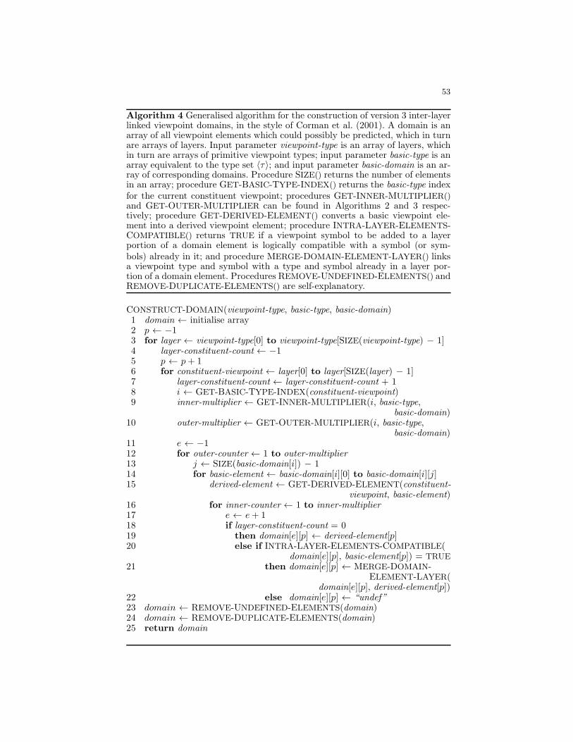
53

Algorithm 4 Generalised algorithm for the construction of version 3 inter-layerlinked viewpoint domains, in the style of Corman et al. (2001). A domain is anarray of all viewpoint elements which could possibly be predicted, which in turnare arrays of layers. Input parameter viewpoint-type is an array of layers, whichin turn are arrays of primitive viewpoint types; input parameter basic-type is anarray equivalent to the type set 〈τ〉; and input parameter basic-domain is an ar-ray of corresponding domains. Procedure SIZE() returns the number of elementsin an array; procedure GET-BASIC-TYPE-INDEX() returns the basic-type indexfor the current constituent viewpoint; procedures GET-INNER-MULTIPLIER()and GET-OUTER-MULTIPLIER can be found in Algorithms 2 and 3 respec-tively; procedure GET-DERIVED-ELEMENT() converts a basic viewpoint ele-ment into a derived viewpoint element; procedure INTRA-LAYER-ELEMENTS-COMPATIBLE() returns TRUE if a viewpoint symbol to be added to a layerportion of a domain element is logically compatible with a symbol (or sym-bols) already in it; and procedure MERGE-DOMAIN-ELEMENT-LAYER() linksa viewpoint type and symbol with a type and symbol already in a layer por-tion of a domain element. Procedures REMOVE-UNDEFINED-ELEMENTS() andREMOVE-DUPLICATE-ELEMENTS() are self-explanatory.

CONSTRUCT-DOMAIN(viewpoint-type, basic-type, basic-domain)1 domain ← initialise array2 p ← −13 for layer ← viewpoint-type[0] to viewpoint-type[SIZE(viewpoint-type) − 1]4 layer-constituent-count ← −15 p ← p+ 16 for constituent-viewpoint ← layer[0] to layer[SIZE(layer) − 1]7 layer-constituent-count ← layer-constituent-count + 18 i ← GET-BASIC-TYPE-INDEX(constituent-viewpoint)9 inner-multiplier ← GET-INNER-MULTIPLIER(i, basic-type,

basic-domain)10 outer-multiplier ← GET-OUTER-MULTIPLIER(i, basic-type,

basic-domain)11 e ← −112 for outer-counter ← 1 to outer-multiplier13 j ← SIZE(basic-domain[i]) − 114 for basic-element ← basic-domain[i][0] to basic-domain[i][j]15 derived-element ← GET-DERIVED-ELEMENT(constituent-

viewpoint, basic-element)16 for inner-counter ← 1 to inner-multiplier17 e ← e+ 118 if layer-constituent-count = 019 then domain[e][p] ← derived-element[p]20 else if INTRA-LAYER-ELEMENTS-COMPATIBLE(

domain[e][p], basic-element[p]) = TRUE21 then domain[e][p] ← MERGE-DOMAIN-

ELEMENT-LAYER(domain[e][p], derived-element[p])

22 else domain[e][p] ← “undef”23 domain ← REMOVE-UNDEFINED-ELEMENTS(domain)24 domain ← REMOVE-DUPLICATE-ELEMENTS(domain)25 return domain

54

〈〈S, 0, Duration, 〈24〉〉〉, 〈〈S, 0, Duration, 〈24〉〉〉,

〈〈S, 0, Duration, 〈24〉〉〉, 〈〈S, 0, Duration, 〈24〉〉〉}.

At this point, the provisional inter-layer linked viewpoint domain contains allof the elements we need (and probably more), albeit that they are incomplete.If there is a second basic or derived viewpoint associated with this layer (i.e.,a constituent of an intra-layer linked viewpoint), then the same procedure isfollowed except that the symbols are linked with the symbols already in theprovisional domain, in the same order as the original additions to the domain.

The for loop beginning on line 6 is executed again, with constituent-viewpointset to Pitch. In line 7, layer-constituent-count is incremented to 1; and in line 8,i is assigned the value 2 (the basic-type index for Pitch). Algorithm 2 returns thedefault value 1, which is assigned to inner-multiplier on line 9. The return valueof Algorithm 3 is the product of the Duration and Cont domain sizes, which is 2.This value is assigned to outer-multiplier on line 10. In line 12, outer-counter isinitially set to 1; and since there are five elements in basic-domain[2] (the Pitchdomain), j is set to 4 in line 13. Variable basic-element is initially assigned thePitch element

〈〈S, 0, Pitch, 〈A♭4〉〉, 〈B, 0, Pitch, 〈F2〉〉〉

in line 14. Since the constituent viewpoint is Pitch, in line 15 derived-element isassigned precisely the same element as basic-element. In line 16, inner-counteris set to 1; and having been initialised as −1 in line 11, e is incremented to 0in line 17. The predicate in line 18 is false; therefore line 20 is executed next.The predicate in this line can only possibly be false if the current layer containsboth Cont and a viewpoint derived from Pitch. In this case, the predicate istrue; therefore line 21 is executed, which replaces the contents of domain[0][0]with 〈S, 0, Duration⊗ Pitch, 〈24, A♭4〉〉. The for loop beginning on line 14is executed a further four times (thereby running through the rest of the Pitch

domain) before executing the for loop beginning on line 12 one more time. Atthis stage the soprano layer has been completed, giving a provisional linkeddomain of

{〈〈S, 0, Duration⊗ Pitch, 〈24, A♭4〉〉〉,

〈〈S, 0, Duration⊗ Pitch, 〈24, A♭4〉〉〉,

〈〈S, 0, Duration⊗ Pitch, 〈24, A♭4〉〉〉,

〈〈S, 0, Duration⊗ Pitch, 〈24, A♭4〉〉〉,

〈〈S, 0, Duration⊗ Pitch, 〈24, A♭4〉〉〉,

〈〈S, 0, Duration⊗ Pitch, 〈24, A♭4〉〉〉,

〈〈S, 0, Duration⊗ Pitch, 〈24, A♭4〉〉〉,

〈〈S, 0, Duration⊗ Pitch, 〈24, A♭4〉〉〉,

〈〈S, 0, Duration⊗ Pitch, 〈24, A♭4〉〉〉,

〈〈S, 0, Duration⊗ Pitch, 〈24, A♭4〉〉〉}.

We then move on to the next layer, again adding to the elements alreadyin the provisional domain, and so on, until all the layers have been dealt with.

55

There is only one other layer in the example, the bass part, which contains theintra-layer linked viewpoint Cont ⊗ ScaleDegree.

The for loop beginning on line 3 is executed again, with layer assigned thearray of viewpoints in the bass layer. Counter p is incremented to 1 in line5; and in the for loop beginning on line 6, constituent-viewpoint is initiallyassigned Cont. Having been initialised as −1 in line 4, layer-constituent-count isincremented to 0 in line 7; and in line 8, i is assigned the value 1 (the basic-typeindex for Cont). The return value of Algorithm 2 is the Pitch domain size, whichis 5. This value is assigned to variable inner-multiplier on line 9. Algorithm 3returns 1 (the size of the Duration domain), which is assigned to variable outer-multiplier on line 10. In line 12, outer-counter is set to 1; and since there are twoelements in basic-domain[1] (the Cont domain), j is set to 1 in line 13. Variablebasic-element is initially assigned the Cont element

〈〈S, 0, Cont, 〈F 〉〉, 〈B, 0, Cont, 〈T 〉〉〉

in line 14. Since the constituent viewpoint is Cont, in line 15 derived-elementis assigned precisely the same element as basic-element. In line 16, in the firstinstance, inner-counter is set to 1; and having been initialised as −1 in line 11,e is incremented to 0 in line 17. The predicate in line 18 is true; therefore line19 is executed, which assigns 〈B, 0, Cont, 〈T 〉〉 to array element domain[0][1].Lines 16 – 19 (inclusive) are executed a further four times, and then the for loopbeginning on line 14 is executed again (thereby processing the remaining Cont

domain element). The provisional linked domain then becomes

{〈〈S, 0, Duration⊗ Pitch, 〈24, A♭4〉〉, 〈B, 0, Cont, 〈T 〉〉〉,

〈〈S, 0, Duration⊗ Pitch, 〈24, A♭4〉〉, 〈B, 0, Cont, 〈T 〉〉〉,

〈〈S, 0, Duration⊗ Pitch, 〈24, A♭4〉〉, 〈B, 0, Cont, 〈T 〉〉〉,

〈〈S, 0, Duration⊗ Pitch, 〈24, A♭4〉〉, 〈B, 0, Cont, 〈T 〉〉〉,

〈〈S, 0, Duration⊗ Pitch, 〈24, A♭4〉〉, 〈B, 0, Cont, 〈T 〉〉〉,

〈〈S, 0, Duration⊗ Pitch, 〈24, A♭4〉〉, 〈B, 0, Cont, 〈F 〉〉〉,

〈〈S, 0, Duration⊗ Pitch, 〈24, A♭4〉〉, 〈B, 0, Cont, 〈F 〉〉〉,

〈〈S, 0, Duration⊗ Pitch, 〈24, A♭4〉〉, 〈B, 0, Cont, 〈F 〉〉〉,

〈〈S, 0, Duration⊗ Pitch, 〈24, A♭4〉〉, 〈B, 0, Cont, 〈F 〉〉〉,

〈〈S, 0, Duration⊗ Pitch, 〈24, A♭4〉〉, 〈B, 0, Cont, 〈F 〉〉〉}.

The final viewpoint to be added is ScaleDegree in the bass part; becauseit predicts Pitch, its inner-multiplier is 1, and its outer-multiplier is 2. Thereis a particular problem to be overcome with respect to the intra-layer linkingof Cont with Pitch, or viewpoints derived from it, however. As we have seenin §6.3, there is an interaction between the Cont and Pitch domains; thereforethe Cartesian product would contain pairings making no logical sense. In thiscase, as the Pitch domain is traversed, the Pitch symbol is checked against therelevant Cont symbol (which is already in the provisional domain): if the pairingmakes logical sense, the Pitch symbol, or a symbol derived from it, is added tothe element in the provisional domain as usual; if not, the element is tagged as

56

undefined. The previous note was F3 (MIDI value 53); therefore 53 is the onlyPitch value which can be sensibly paired with a Cont value of T . The tonic isE♭; therefore F has a ScaleDegree value of 2.

The for loop beginning on line 6 is executed again, with constituent-viewpointset to ScaleDegree. In line 7, layer-constituent-count is incremented to 1; andin line 8, i is assigned the value 2 (the basic-type index for Pitch). Algorithm 2returns the default value 1, which is assigned to inner-multiplier on line 9. Thereturn value of Algorithm 3 is the product of the Duration and Cont domainsizes, which is 2. This value is assigned to outer-multiplier on line 10. In line12, outer-counter is initially set to 1; and since there are five elements in basic-domain[2] (the Pitch domain), j is set to 4 in line 13. Variable basic-element isinitially assigned the Pitch element

〈〈S, 0, Pitch, 〈A♭4〉〉, 〈B, 0, Pitch, 〈F2〉〉〉

in line 14. This time, since the constituent viewpoint is ScaleDegree, in line 15derived-element is assigned the element

〈〈S, 0, ScaleDegree, 〈5〉〉, 〈B, 0, ScaleDegree, 〈2〉〉〉.

In line 16, inner-counter is set to 1; and having been initialised as −1 in line 11,e is incremented to 0 in line 17. The predicate in line 18 is false; therefore line 20is executed next. The predicate in this line is false, because F3 followed by F2 isnot compatible with a Cont value of T (it is assumed that previous predictionshave global scope; that is, they can be accessed from anywhere); therefore line 22is executed, in which the contents of domain[0][1] are replaced with undef. Thefor loop beginning on line 14 is executed a further four times, thereby runningthrough the rest of the Pitch domain. The predicate in line 20 is true on onlyone of these passes (when F3 is followed by F3), in which case the contents ofdomain[3][1] are replaced with 〈B, 0, Cont ⊗ ScaleDegree, 〈T, 2〉〉. The forloop beginning on line 12 is executed one more time, giving a provisional linkeddomain of

{〈〈S, 0, Duration⊗ Pitch, 〈24, A♭4〉〉, undef 〉,

〈〈S, 0, Duration⊗ Pitch, 〈24, A♭4〉〉, undef 〉,

〈〈S, 0, Duration⊗ Pitch, 〈24, A♭4〉〉, undef 〉,

〈〈S, 0, Duration⊗ Pitch, 〈24, A♭4〉〉, 〈B, 0, Cont⊗ ScaleDegree, 〈T, 2〉〉〉,

〈〈S, 0, Duration⊗ Pitch, 〈24, A♭4〉〉, undef 〉,

〈〈S, 0, Duration⊗ Pitch, 〈24, A♭4〉〉, 〈B, 0, Cont⊗ ScaleDegree, 〈F, 2〉〉〉,

〈〈S, 0, Duration⊗ Pitch, 〈24, A♭4〉〉, 〈B, 0, Cont⊗ ScaleDegree, 〈F, 0〉〉〉,

〈〈S, 0, Duration⊗ Pitch, 〈24, A♭4〉〉, 〈B, 0, Cont⊗ ScaleDegree, 〈F, 1〉〉〉,

〈〈S, 0, Duration⊗ Pitch, 〈24, A♭4〉〉, 〈B, 0, Cont⊗ ScaleDegree, 〈F, 2〉〉〉,

〈〈S, 0, Duration⊗ Pitch, 〈24, A♭4〉〉, 〈B, 0, Cont⊗ ScaleDegree, 〈F, 3〉〉〉}.

The provisional domain, constructed in this way in order to ensure thatsymbols which do not correspond with each other are not linked, may containelements tagged as undefined, and may also contain duplicate elements; therefore

57

the final inter-layer linked viewpoint domain is achieved once undefined andduplicate elements have been removed (lines 23 and 24):

{〈〈S, 0, Duration⊗ Pitch, 〈24, A♭4〉〉, 〈B, 0, Cont⊗ ScaleDegree, 〈T, 2〉〉〉,

〈〈S, 0, Duration⊗ Pitch, 〈24, A♭4〉〉, 〈B, 0, Cont⊗ ScaleDegree, 〈F, 0〉〉〉,

〈〈S, 0, Duration⊗ Pitch, 〈24, A♭4〉〉, 〈B, 0, Cont⊗ ScaleDegree, 〈F, 1〉〉〉,

〈〈S, 0, Duration⊗ Pitch, 〈24, A♭4〉〉, 〈B, 0, Cont⊗ ScaleDegree, 〈F, 2〉〉〉,

〈〈S, 0, Duration⊗ Pitch, 〈24, A♭4〉〉, 〈B, 0, Cont⊗ ScaleDegree, 〈F, 3〉〉〉}.