1

Multiple Testing Issues with

Gene Expression Data

Utah State University – Spring 2014

STAT 5570: Statistical Bioinformatics

Notes 3.1

2

References

Chapter 15 of Bioconductor Monograph

(course text)

Benjamini & Hochberg (1995) J. of the Royal

Stat. Soc., series B, 57(1):289-300

Storey & Tibshirani (2003) Proc. of the Natl.

Acad. of Science, 100(16):9440-9445

3

Where are we?

Up to now:

Intro. to microarray technology and estimating gene expression levels (preprocessing)

Clustering and visualization (sometimes using a specific subset of genes)

Coming up:

Testing for differential expression (DE)

finding a subset of “significant” genes

Annotation and online resources

Technologies other than microarrays

Here: what to do with DE test results

4

Differential Expression (DE) tests – basics

Have 2 or more groups of samples

ex: healthy, beg. disease, adv. disease

Null: Gene expressed same in all groups

Alt.: Gene not expressed same in all groups

(biological relevance?)

Result:

Test Stat.: some “standardized” measure of DE

– like a t-test, maybe

P-value: some measure of “significance”

5

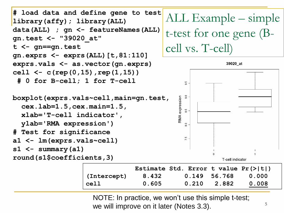
ALL Example – simple

t-test for one gene (B-

cell vs. T-cell)

# load data and define gene to test

library(affy); library(ALL)

data(ALL) ; gn <- featureNames(ALL)

gn.test <- "39020_at"

t <- gn==gn.test

gn.exprs <- exprs(ALL)[t,81:110]

exprs.vals <- as.vector(gn.exprs)

cell <- c(rep(0,15),rep(1,15))

# 0 for B-cell; 1 for T-cell

boxplot(exprs.vals~cell,main=gn.test,

cex.lab=1.5,cex.main=1.5,

xlab='T-cell indicator',

ylab='RMA expression')

# Test for significance

a1 <- lm(exprs.vals~cell)

s1 <- summary(a1)

round(s1$coefficients,3)

NOTE: In practice, we won’t use this simple t-test;

we will improve on it later (Notes 3.3).

Estimate Std. Error t value Pr(>|t|)

(Intercept) 8.432 0.149 56.768 0.000

cell 0.605 0.210 2.882 0.008

6

Significance and P-values

Usually, “small” P-value claim significance

Correct interpretation of P-value from a test of significance:

“The probability of obtaining a difference

at least as extreme as what wasobserved, just by chance when the nullhypothesis is true.”

Consider a t-test of H0: μ0-μ1=0, when in reality, μ0-μ1 = c (and SD=1 for both pop.)

What P-values are possible, and how likely are they?

7

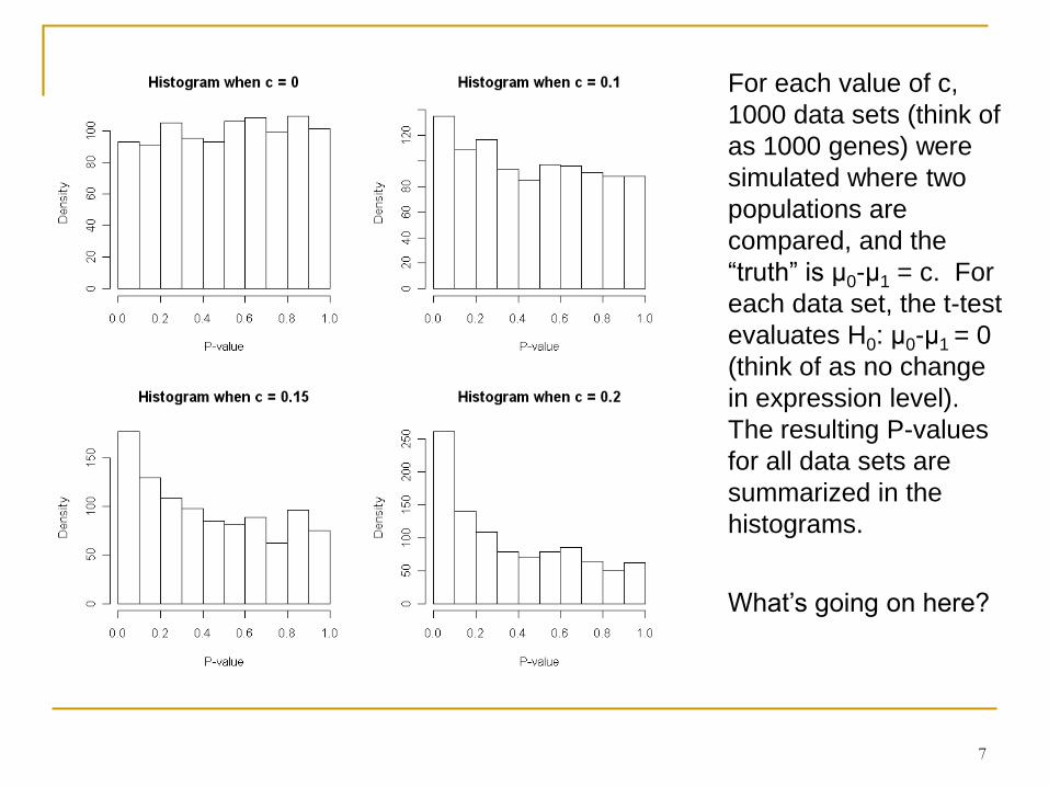
For each value of c,

1000 data sets (think of

as 1000 genes) were

simulated where two

populations are

compared, and the

“truth” is μ0-μ1 = c. For

each data set, the t-test

evaluates H0: μ0-μ1 = 0

(think of as no change

in expression level).

The resulting P-values

for all data sets are

summarized in the

histograms.

What’s going on here?

8

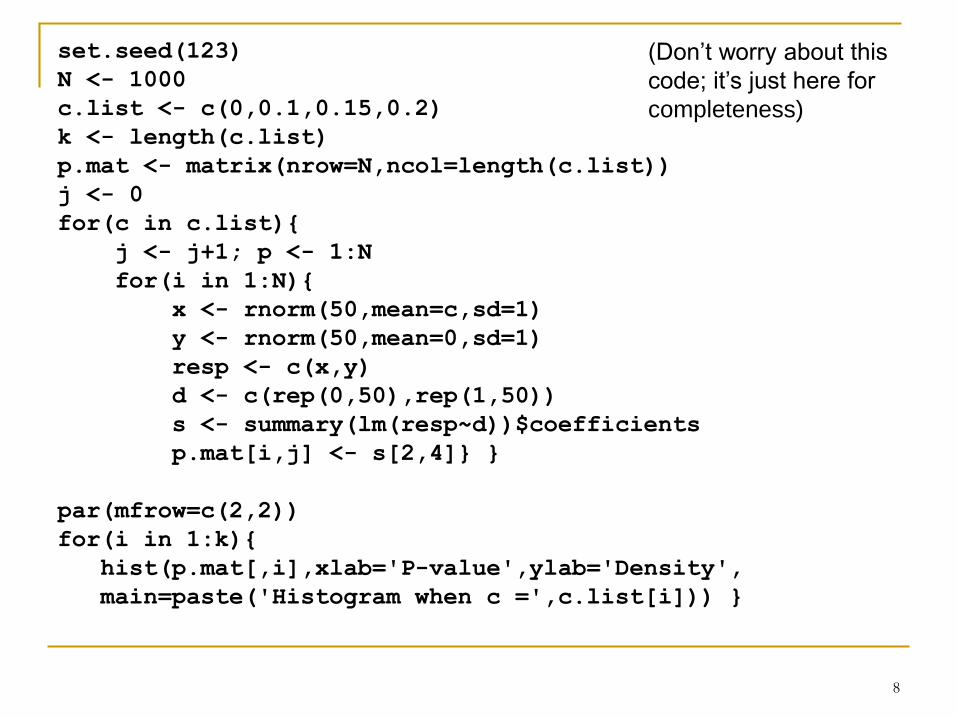
set.seed(123)

N <- 1000

c.list <- c(0,0.1,0.15,0.2)

k <- length(c.list)

p.mat <- matrix(nrow=N,ncol=length(c.list))

j <- 0

for(c in c.list){

j <- j+1; p <- 1:N

for(i in 1:N){

x <- rnorm(50,mean=c,sd=1)

y <- rnorm(50,mean=0,sd=1)

resp <- c(x,y)

d <- c(rep(0,50),rep(1,50))

s <- summary(lm(resp~d))$coefficients

p.mat[i,j] <- s[2,4]} }

par(mfrow=c(2,2))

for(i in 1:k){

hist(p.mat[,i],xlab='P-value',ylab='Density',

main=paste('Histogram when c =',c.list[i])) }

(Don’t worry about this

code; it’s just here for

completeness)

9

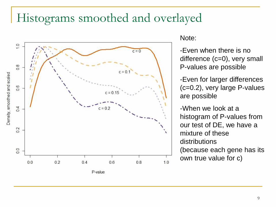
Note:

-Even when there is no

difference (c=0), very small

P-values are possible

-Even for larger differences

(c=0.2), very large P-values

are possible

-When we look at a

histogram of P-values from

our test of DE, we have a

mixture of these

distributions

(because each gene has its

own true value for c)

Histograms smoothed and overlayed

10

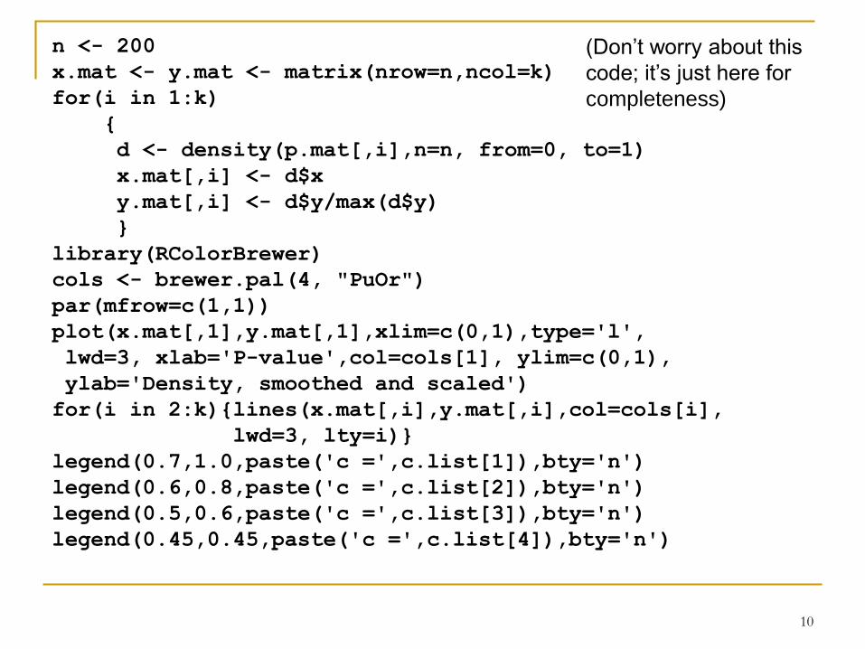
n <- 200

x.mat <- y.mat <- matrix(nrow=n,ncol=k)

for(i in 1:k)

{

d <- density(p.mat[,i],n=n, from=0, to=1)

x.mat[,i] <- d$x

y.mat[,i] <- d$y/max(d$y)

}

library(RColorBrewer)

cols <- brewer.pal(4, "PuOr")

par(mfrow=c(1,1))

plot(x.mat[,1],y.mat[,1],xlim=c(0,1),type='l',

lwd=3, xlab='P-value',col=cols[1], ylim=c(0,1),

ylab='Density, smoothed and scaled')

for(i in 2:k){lines(x.mat[,i],y.mat[,i],col=cols[i],

lwd=3, lty=i)}

legend(0.7,1.0,paste('c =',c.list[1]),bty='n')

legend(0.6,0.8,paste('c =',c.list[2]),bty='n')

legend(0.5,0.6,paste('c =',c.list[3]),bty='n')

legend(0.45,0.45,paste('c =',c.list[4]),bty='n')

(Don’t worry about this

code; it’s just here for

completeness)

11

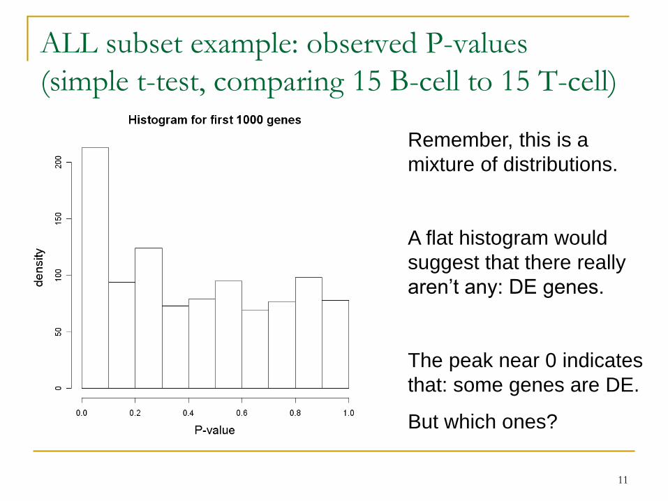
ALL subset example: observed P-values

(simple t-test, comparing 15 B-cell to 15 T-cell)

Remember, this is a

mixture of distributions.

A flat histogram would

suggest that there really

aren’t any: DE genes.

The peak near 0 indicates

that: some genes are DE.

But which ones?

12

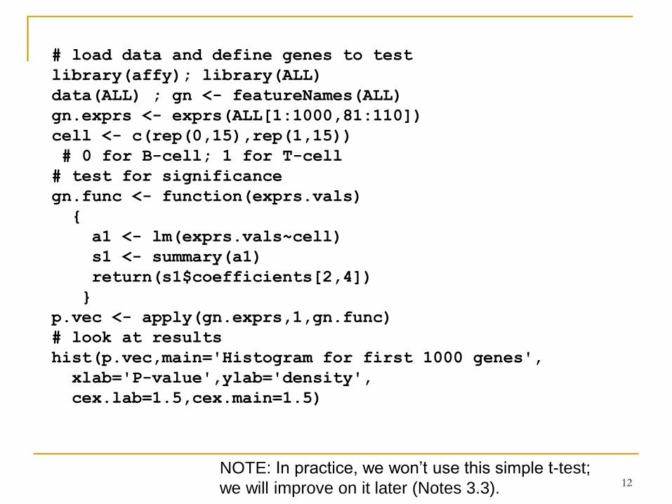
# load data and define genes to test

library(affy); library(ALL)

data(ALL) ; gn <- featureNames(ALL)

gn.exprs <- exprs(ALL[1:1000,81:110])

cell <- c(rep(0,15),rep(1,15))

# 0 for B-cell; 1 for T-cell

# test for significance

gn.func <- function(exprs.vals)

{

a1 <- lm(exprs.vals~cell)

s1 <- summary(a1)

return(s1$coefficients[2,4])

}

p.vec <- apply(gn.exprs,1,gn.func)

# look at results

hist(p.vec,main='Histogram for first 1000 genes',

xlab='P-value',ylab='density',

cex.lab=1.5,cex.main=1.5)

NOTE: In practice, we won’t use this simple t-test;

we will improve on it later (Notes 3.3).

13

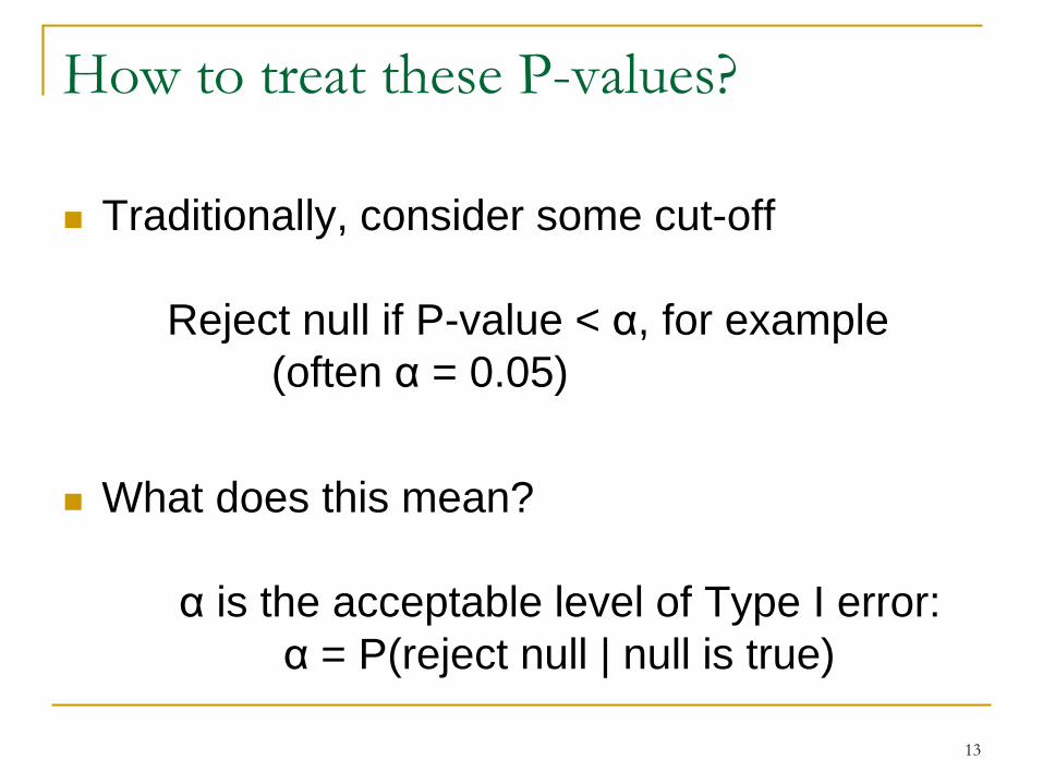
How to treat these P-values?

Traditionally, consider some cut-off

Reject null if P-value < α, for example

(often α = 0.05)

What does this mean?

α is the acceptable level of Type I error:

α = P(reject null | null is true)

14

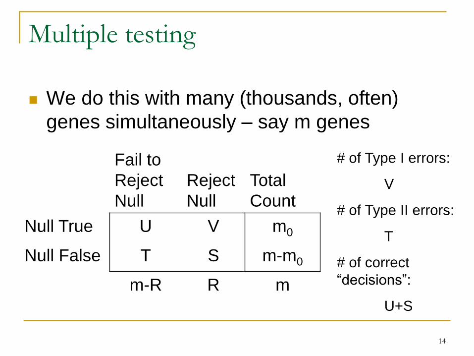
Multiple testing

We do this with many (thousands, often)

genes simultaneously – say m genes

Fail to

Reject

Null

Reject

Null

Total

Count

Null True U V m0

Null False T S m-m0

m-R R m

# of Type I errors:

V

# of Type II errors:

T

# of correct

“decisions”:

U+S

15

Error rates

Think of this as a family of m tests or

comparisons

Per-comparison error rate: PCER = E[V/m]

Family-wise error rate: FWER = P(V ≥ 1)

What does the α-cutoff mean here?

Testing each hypothesis (gene) at level α

guarantees:

PCER ≤ α

- let’s look at why

16

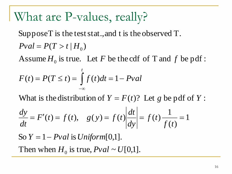
What are P-values, really?

].1,0[~ true,is whenThen

].1,0[ is 1 So

1)(

1)()()( ,)()(

: of pdf be Let ?)( of ondistributi theisWhat

1)()()(

:pdf be and T of cdf thebe Let true.is Assume

)|(

T. observed theis t and stat., test theis T Suppose

0

0

0

UPvalH

UniformPvalY

tftf

dy

dttfygtftF

dt

dy

YgtFY

PvaldttftTPtF

fFH

HtTPPval

t

17

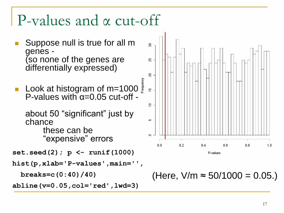
P-values and α cut-off

Suppose null is true for all m genes -(so none of the genes are differentially expressed)

Look at histogram of m=1000 P-values with α=0.05 cut-off -

about 50 “significant” just by chance

these can be“expensive” errors

set.seed(2); p <- runif(1000)

hist(p,xlab='P-values',main='',

breaks=c(0:40)/40)

abline(v=0.05,col='red',lwd=3)

(Here, V/m ≈ 50/1000 = 0.05.)

18

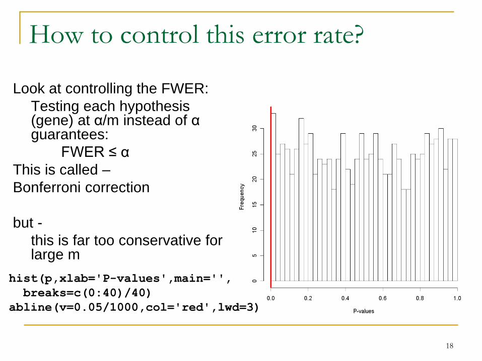
How to control this error rate?

Look at controlling the FWER:

Testing each hypothesis (gene) at α/m instead of αguarantees:

FWER ≤ α

This is called –

Bonferroni correction

but -

this is far too conservative for large m

hist(p,xlab='P-values',main='',

breaks=c(0:40)/40)

abline(v=0.05/1000,col='red',lwd=3)

19

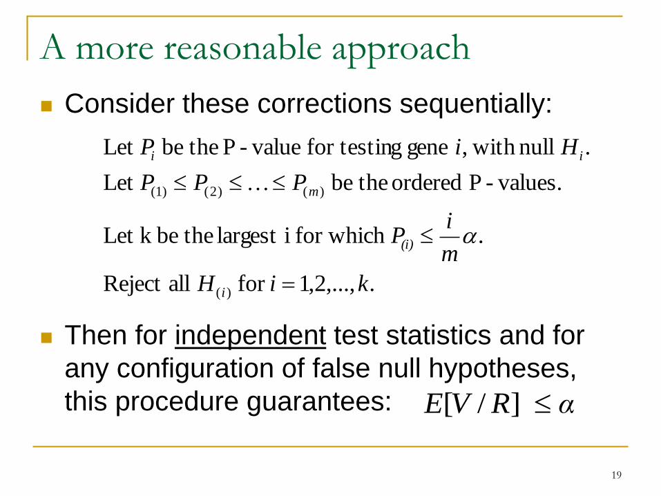
A more reasonable approach

Consider these corrections sequentially:

Then for independent test statistics and for

any configuration of false null hypotheses,

this procedure guarantees:

.,...,2,1for allReject

. for which ilargest thebek Let

values.- Pordered thebe Let

. null with, gene gfor testin value- P thebe Let

)(

)()2()1(

kiH

m

iP

PPP

HiP

i

(i)

m

ii

α RVE ]/[

20

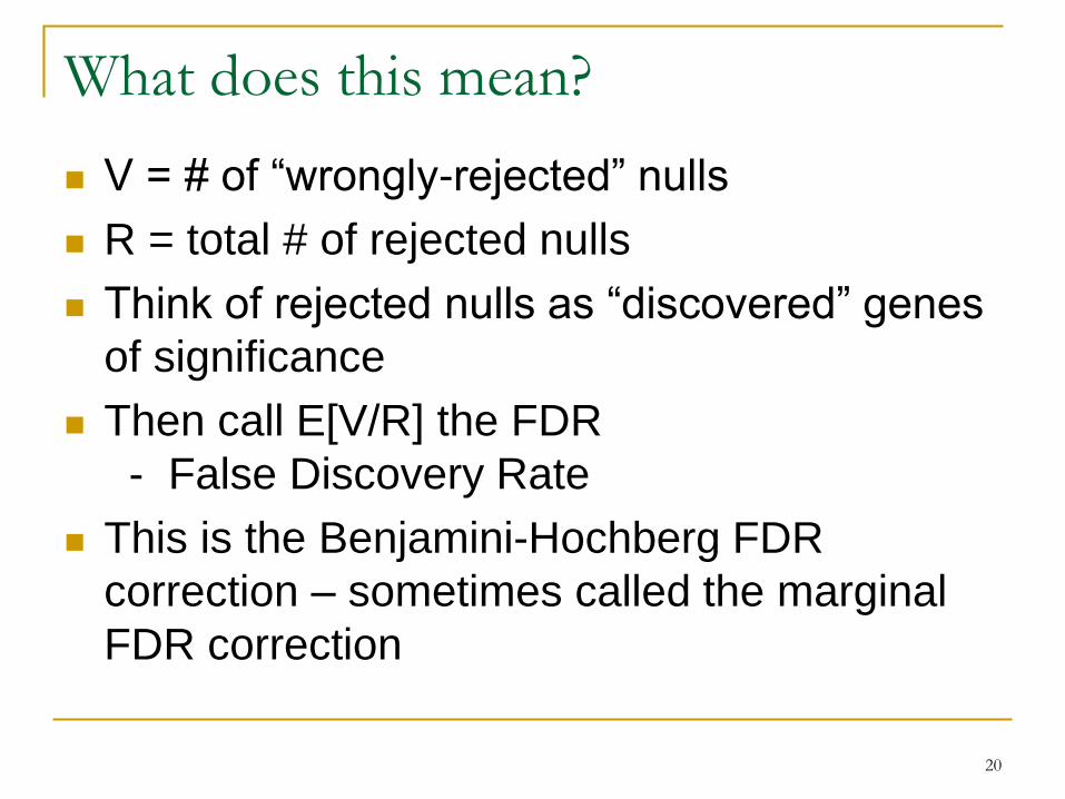
What does this mean?

V = # of “wrongly-rejected” nulls

R = total # of rejected nulls

Think of rejected nulls as “discovered” genes

of significance

Then call E[V/R] the FDR

- False Discovery Rate

This is the Benjamini-Hochberg FDR

correction – sometimes called the marginal

FDR correction

21

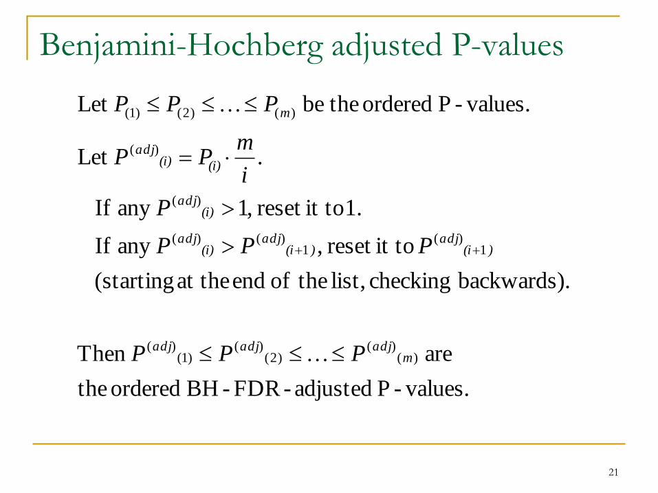
Benjamini-Hochberg adjusted P-values

values.-P adjusted-FDR-BH ordered the

are Then

.backwards) checking list, theof end at the (starting

it toreset ,any If

1. it toreset ,1any If

.Let

values.-P ordered thebe Let

)()(

)2()(

)1()(

1)(

1)()(

)(

)(

)()2()1(

madjadjadj

)(iadj

)(iadj

(i)adj

(i)adj

(i)(i)adj

m

PPP

PPP

P

i

mPP

PPP

22

An extension: the q-value

P-value for a gene:

the probability of observing a test stat.

more extreme when null is true

q-value for a gene:

the expected proportion of false positives

incurred when calling that gene significant

Compare (with slight abuse of notation):

)| true( ) true|( 00 tTHPqvalHtTPpval

23

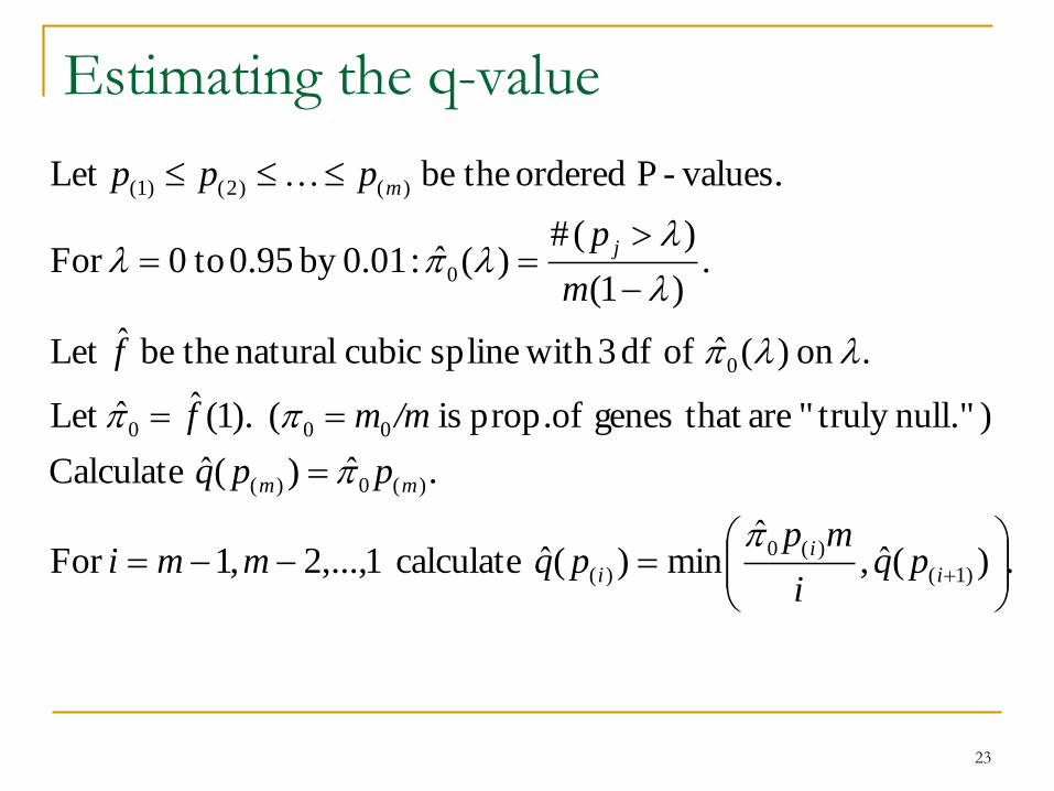
Estimating the q-value

.)(ˆ,ˆ

min)(ˆ calculate 1,...,2,1For

.ˆ)(ˆ Calculate

)null."truly " are that genes of prop. is ( ).1(ˆˆLet

. on )(ˆ of df 3 withspline cubic natural thebe ˆLet

.)1(

)(#)(ˆ :0.01by 0.95 to0For

values.- Pordered thebe Let

)1(

)(0

)(

)(0)(

000

0

0

)()2()1(

i

i

i

mm

j

m

pqi

mppqmmi

ppq

/mmf

f

m

p

ppp

24

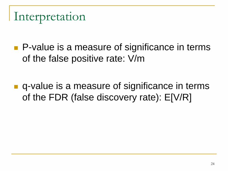
Interpretation

P-value is a measure of significance in terms

of the false positive rate: V/m

q-value is a measure of significance in terms

of the FDR (false discovery rate): E[V/R]

25

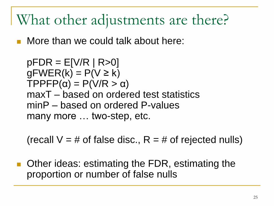
What other adjustments are there?

More than we could talk about here:

pFDR = E[V/R | R>0] gFWER(k) = P(V ≥ k)TPPFP(α) = P(V/R > α)maxT – based on ordered test statisticsminP – based on ordered P-valuesmany more … two-step, etc.

(recall V = # of false disc., R = # of rejected nulls)

Other ideas: estimating the FDR, estimating the proportion or number of false nulls

26

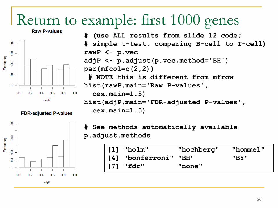
# (use ALL results from slide 12 code;

# simple t-test, comparing B-cell to T-cell)

rawP <- p.vec

adjP <- p.adjust(p.vec,method='BH')

par(mfcol=c(2,2))

# NOTE this is different from mfrow

hist(rawP,main='Raw P-values',

cex.main=1.5)

hist(adjP,main='FDR-adjusted P-values',

cex.main=1.5)

# See methods automatically available

p.adjust.methods

Return to example: first 1000 genes

[1] "holm" "hochberg" "hommel"

[4] "bonferroni" "BH" "BY"

[7] "fdr" "none"

27

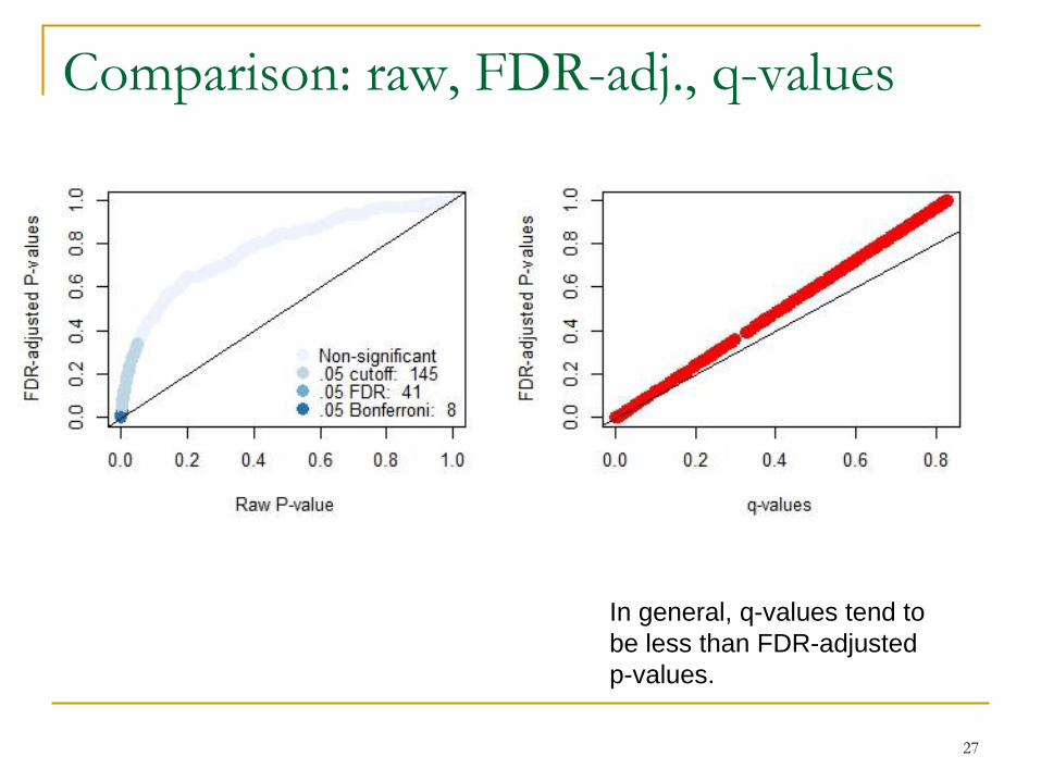
Comparison: raw, FDR-adj., q-values

In general, q-values tend to

be less than FDR-adjusted

p-values.

28

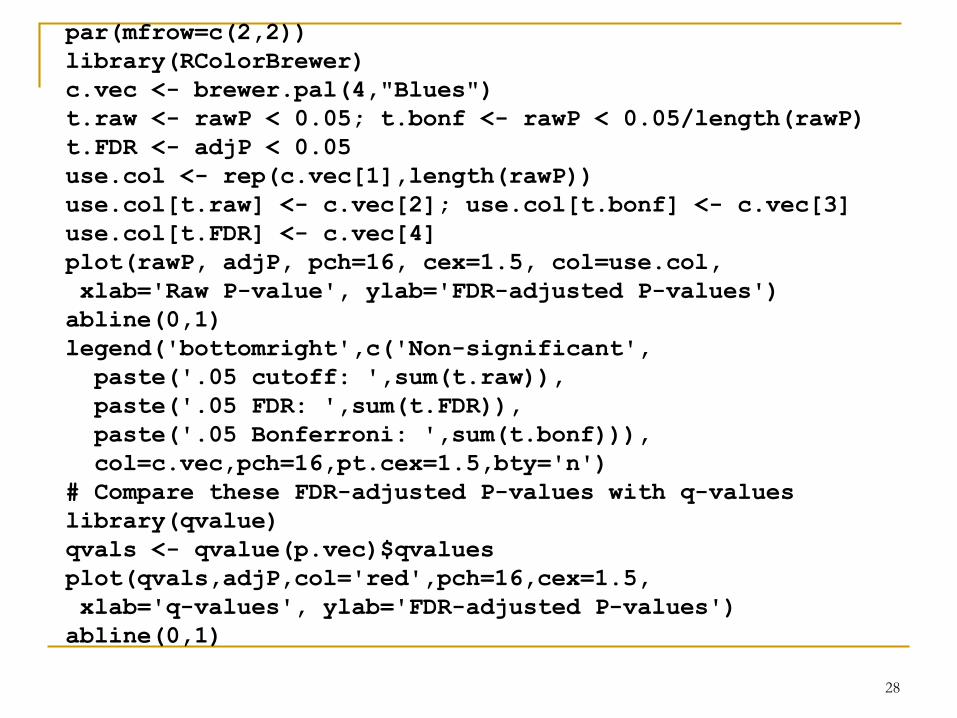
par(mfrow=c(2,2))

library(RColorBrewer)

c.vec <- brewer.pal(4,"Blues")

t.raw <- rawP < 0.05; t.bonf <- rawP < 0.05/length(rawP)

t.FDR <- adjP < 0.05

use.col <- rep(c.vec[1],length(rawP))

use.col[t.raw] <- c.vec[2]; use.col[t.bonf] <- c.vec[3]

use.col[t.FDR] <- c.vec[4]

plot(rawP, adjP, pch=16, cex=1.5, col=use.col,

xlab='Raw P-value', ylab='FDR-adjusted P-values')

abline(0,1)

legend('bottomright',c('Non-significant',

paste('.05 cutoff: ',sum(t.raw)),

paste('.05 FDR: ',sum(t.FDR)),

paste('.05 Bonferroni: ',sum(t.bonf))),

col=c.vec,pch=16,pt.cex=1.5,bty='n')

# Compare these FDR-adjusted P-values with q-values

library(qvalue)

qvals <- qvalue(p.vec)$qvalues

plot(qvals,adjP,col='red',pch=16,cex=1.5,

xlab='q-values', ylab='FDR-adjusted P-values')

abline(0,1)

Which error rate?

Type I: call gene ‘candidate’ when it’s not

PCER / FWER / FDR / etc.

Type II: fail to identify true candidate

Relative value (I vs. II) depends on perspective

Wasted effort

Lost opportunity

How to reconcile?

Sample size power low Type II

Statistical method low Type I

29

Current Areas of Research

Controlling error rates with multiple

dependent tests

Controlling error rates in multiple structured

hypotheses (e.g., nested or conditional tests)

Choosing an appropriate family

(within which collection of tests should error rates

be controlled?)

30

31

Summary

Tests of differential expression

Null: gene is not DE

Alt: gene is DE

Test Stat. P-value

How to treat P-values: uniform random variables

Multiple comparison procedures

simple cut-off too liberal

Bonferroni correction too conservative

FWER

FDR and q-values

others – we may return to this topic: good 6570 projects