Multiple Regression

Class 22

Multiple Regression (MR)

Y = bo + b1 + b2 + b3 + ……bx + ε

Multiple regression (MR) can incorporate any number of predictors in model.

“Regression plane” with 2 predictors, after that it becomes increasingly difficult to visualize result.

MR operates on same principles as simple regression.

Multiple R = correlation between observed Y and Y as predicted by total model (i.e., all predictors at once).

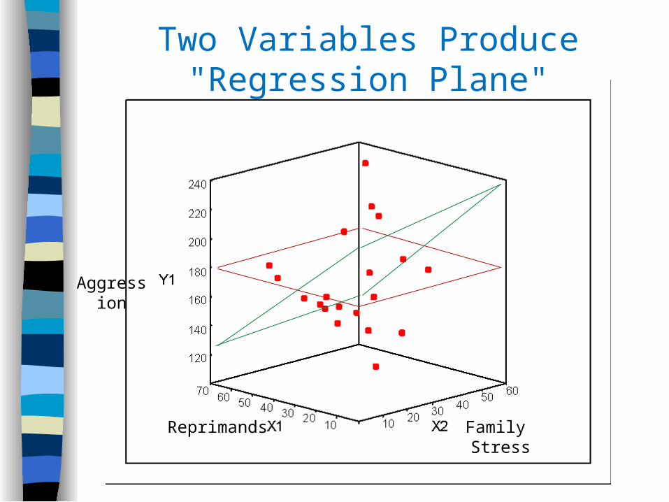
Two Variables Produce "Regression Plane"

Aggression

Reprimands Family Stress

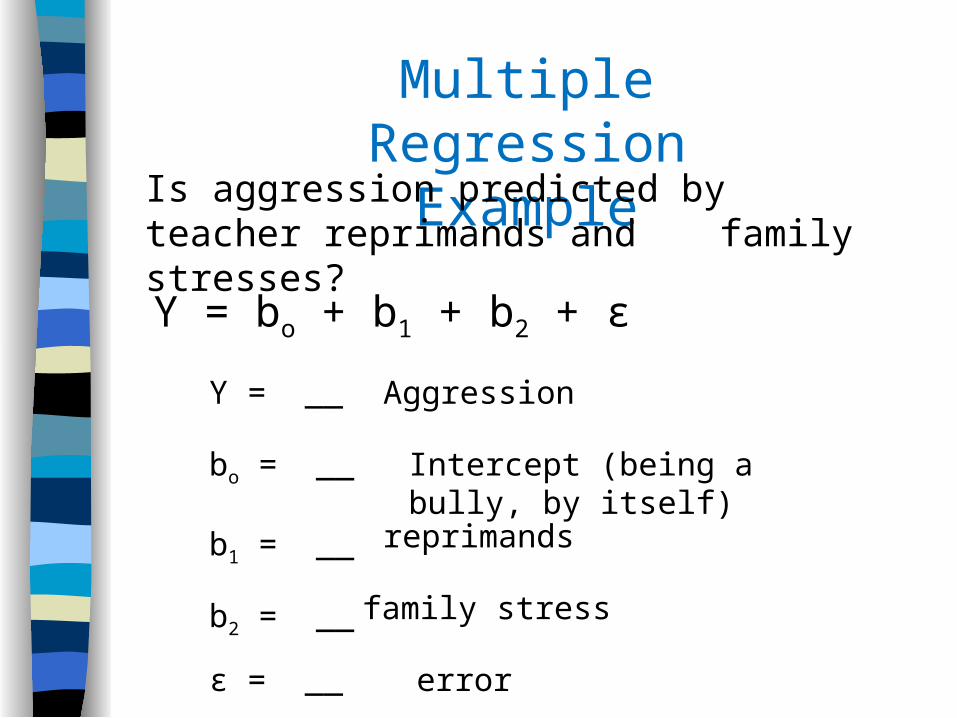
Multiple Regression Example

Is aggression predicted by teacher reprimands and family stresses?

Y = bo + b1 + b2 + ε

Y = __

bo = __

b1 = __

b2 = __

ε = __

Aggression

Intercept (being a bully, by itself)

family stress

reprimands

error

Elements of Multiple RegressionTotal Sum of Squares (SST) = Deviation of each score from DV mean,

square these deviations, then sum them.

Residual Sum of Squares (SSR) = Each residual from total model (not simple line), squared, then sum all these squared residuals.

Model Sum of Squares (SSM) = SST – SSR = The amount that the total model explains result above and beyond the simple mean.

R2 = SSM / SST = Proportion of variance explained, by the total model.

Adjusted R2 = R2, but adjusted to having multiple predictors

NOTE: Main diff. between these values in mutli. regression and simple regression is use of total model rather than single slope. Math much more complicated, but conceptually the same.

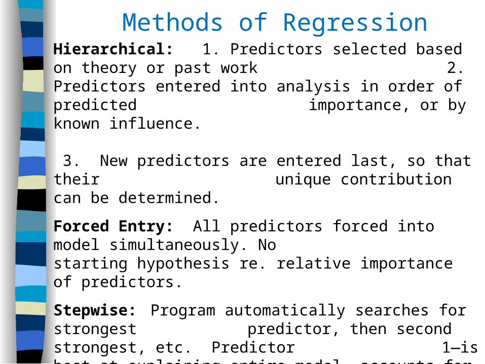
Methods of RegressionHierarchical: 1. Predictors selected based on theory or past work

2. Predictors entered into analysis in order of predicted importance, or by known influence.

3. New predictors are entered last, so that their unique contribution can be determined.

Forced Entry: All predictors forced into model simultaneously. No starting hypothesis re. relative importance of predictors.

Stepwise: Program automatically searches for strongest predictor, then second strongest, etc. Predictor 1—is best at explaining entire model, accounts for say 40% . Predictor 2 is best at explaining remaining 60%, etc. Controversial method.

In general, Hierarchical is most common and most accepted.

Avoid “kitchen sink” Limit number of predictors to few as possible, and to those that make theoretical sense.

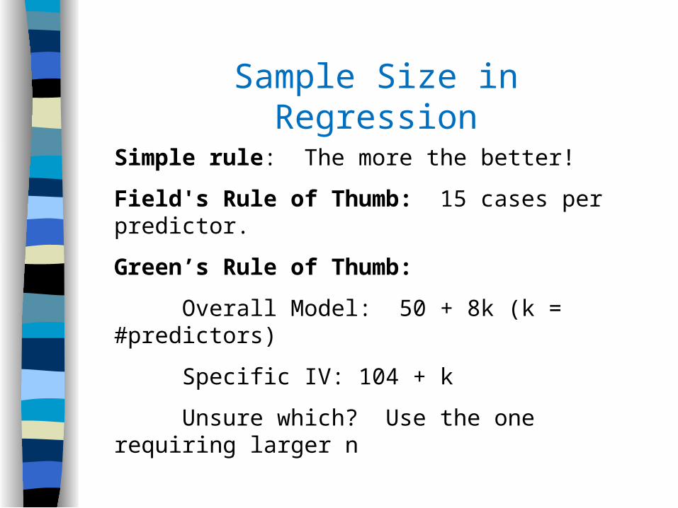
Sample Size in Regression

Simple rule: The more the better!

Field's Rule of Thumb: 15 cases per predictor.

Green’s Rule of Thumb:

Overall Model: 50 + 8k (k = #predictors)

Specific IV: 104 + k

Unsure which? Use the one requiring larger n

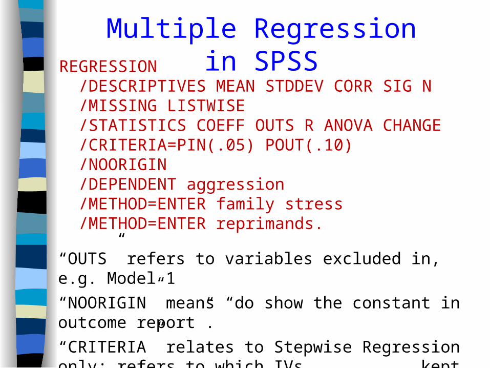
Multiple Regression in SPSS

“OUTS” refers to variables excluded in, e.g. Model 1“NOORIGIN” means “do show the constant in outcome report”.“CRITERIA” relates to Stepwise Regression only; refers to which IVs

kept in at Step 1, Step 2, etc.

REGRESSION /DESCRIPTIVES MEAN STDDEV CORR SIG N /MISSING LISTWISE /STATISTICS COEFF OUTS R ANOVA CHANGE /CRITERIA=PIN(.05) POUT(.10) /NOORIGIN /DEPENDENT aggression /METHOD=ENTER family stress /METHOD=ENTER reprimands.

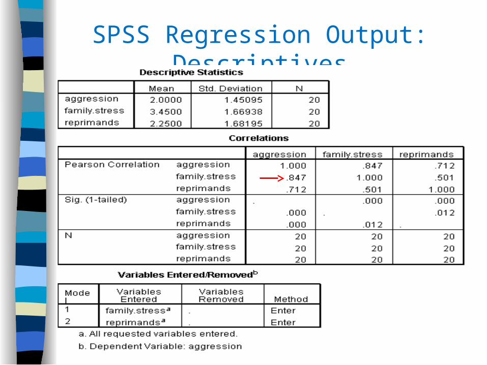
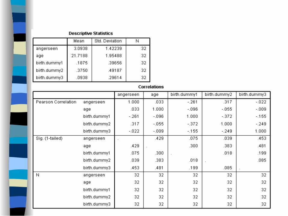
SPSS Regression Output: Descriptives

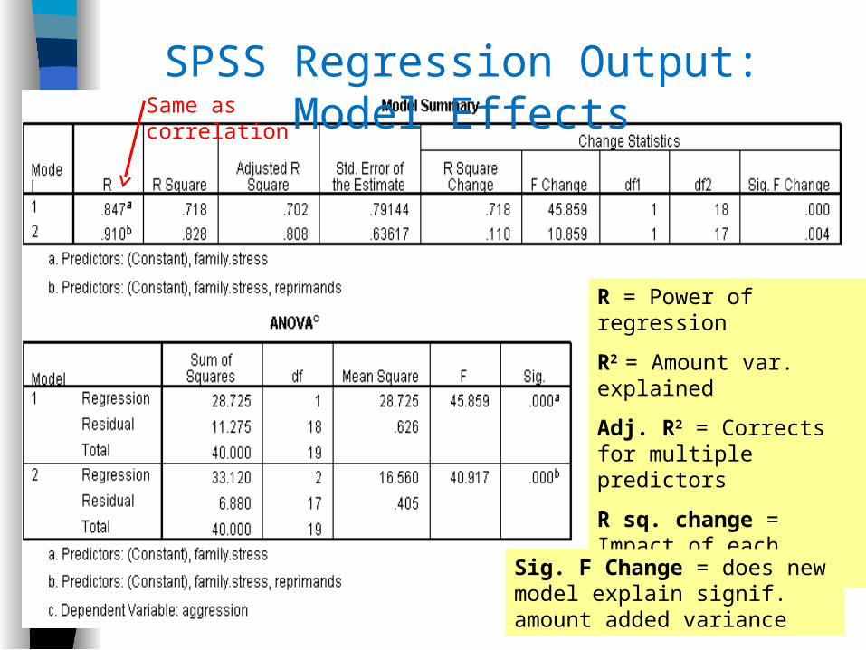
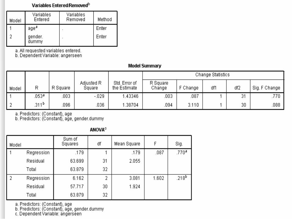
SPSS Regression Output: Model EffectsSame as correlation

R = Power of regression

R2 = Amount var. explained

Adj. R2 = Corrects for multiple predictors

R sq. change = Impact of each added model

Sig. F Change = does new model explain signif. amount added variance

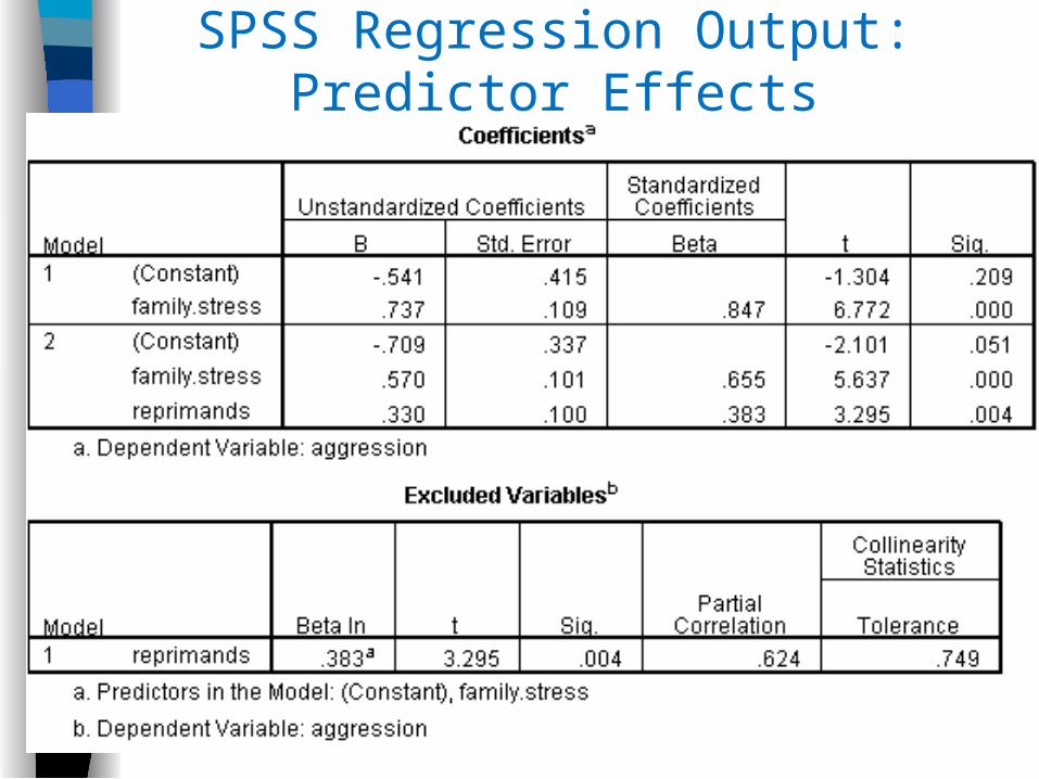
SPSS Regression Output: Predictor Effects

Requirements and Assumptions (these apply to Simple and Multiple Regression)

Variable Types: Predictors must be quantitative or categorical (2 values only, i.e. dichotomous); Outcomes must be interval.

Non-Zero Variance: Predictors have variation in value.

No Perfect multicollinearity: No perfect 1:1 (linear) relationship between 2 or more predictors.

Predictors uncorrelated to external variables: No hidden “third variable” confounds

Homoscedasticity: Variance at each level of predictor is constant.

Requirements and Assumptions (continued)

Independent Errors (no auto-correlation): Residuals for Sub. 1 do not determine residuals for Sub. 2. Durbin-Watson > 1 and < 3

Normally Distributed Errors: Residuals are random, and sum to zero (or close to zero).

Independence: All outcome values are independent from one another, i.e., each response comes from a subject who is uninfluenced by other subjects. Subs

Linearity: The changes in outcome due to each predictor are described best by a straight line.

Multicollinearity

In multiple regression, statistic assumes that each new predictor is in fact a unique measure.

If two predictors, A and B, are very highly correlated, then a model testing the added affect of Predictor B might, in effect, be testing Predictor A twice.

The slopes of each variable are not orthogonal (go in different directions, but instead run parallel to each other (i.e., they are co-linear).

Mac Collinearity: A Multicollinearity Saga

Suffering negative publicity regarding the health risks of fast food, the fast food industry hires the research firm of Fryes, Berger, and Shaque (FBS) to show that there is no intrinsic harm in fast food.

FBS surveys a random sample, and asks:

a.To what degree are you a meat eater? (Carnivore)b.How often do you purchase fast food? (Fast.food)c.What is your health status? (Health) FBS conducts a multiple regression, entering fast.food in step one and carnivore in step 2.

"AHA!", they shout, "there is no problem with fast food—its just that so many carnivores for some reason go to fast food restaurants!"

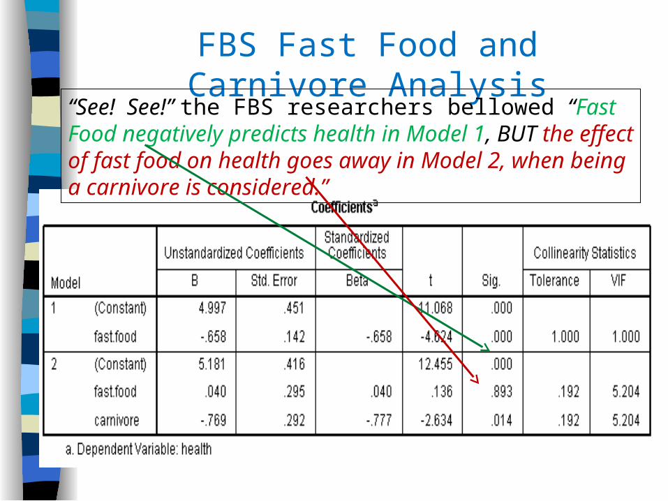
FBS Fast Food and Carnivore Analysis

“See! See!” the FBS researchers bellowed “Fast Food negatively predicts health in Model 1, BUT the effect of fast food on health goes away in Model 2, when being a carnivore is considered.”

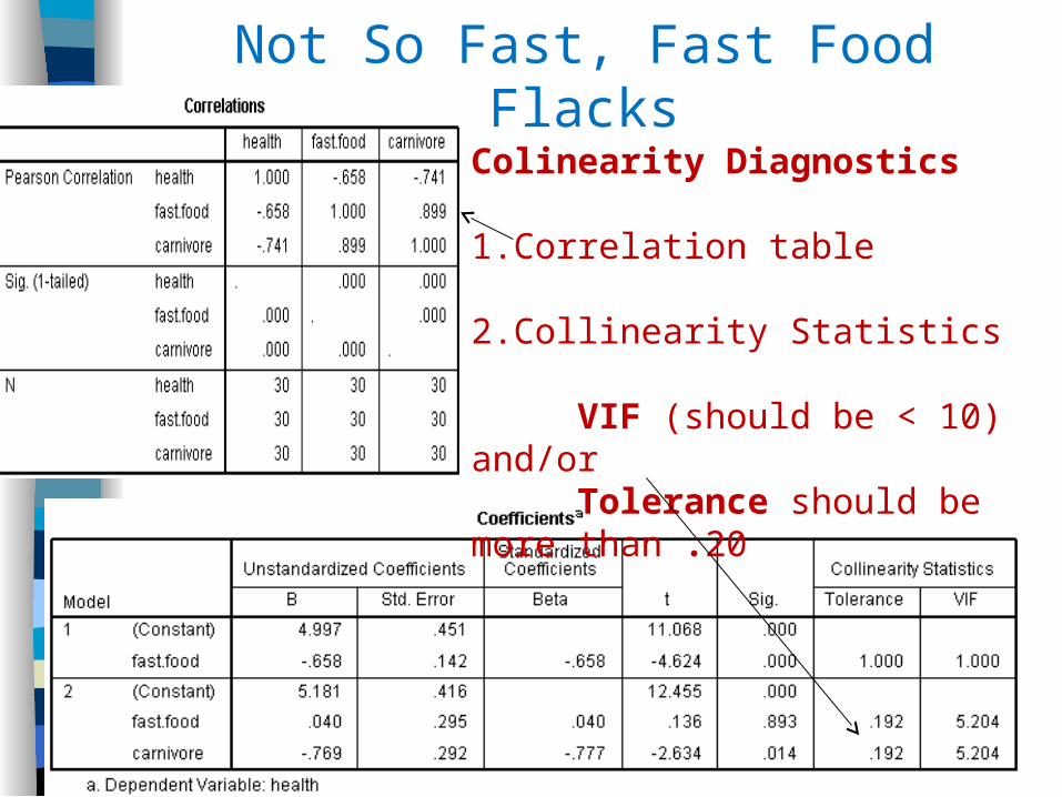
Not So Fast, Fast Food Flacks

Colinearity Diagnostics 1.Correlation table

2.Collinearity Statistics

VIF (should be < 10) and/orTolerance should be more than .20

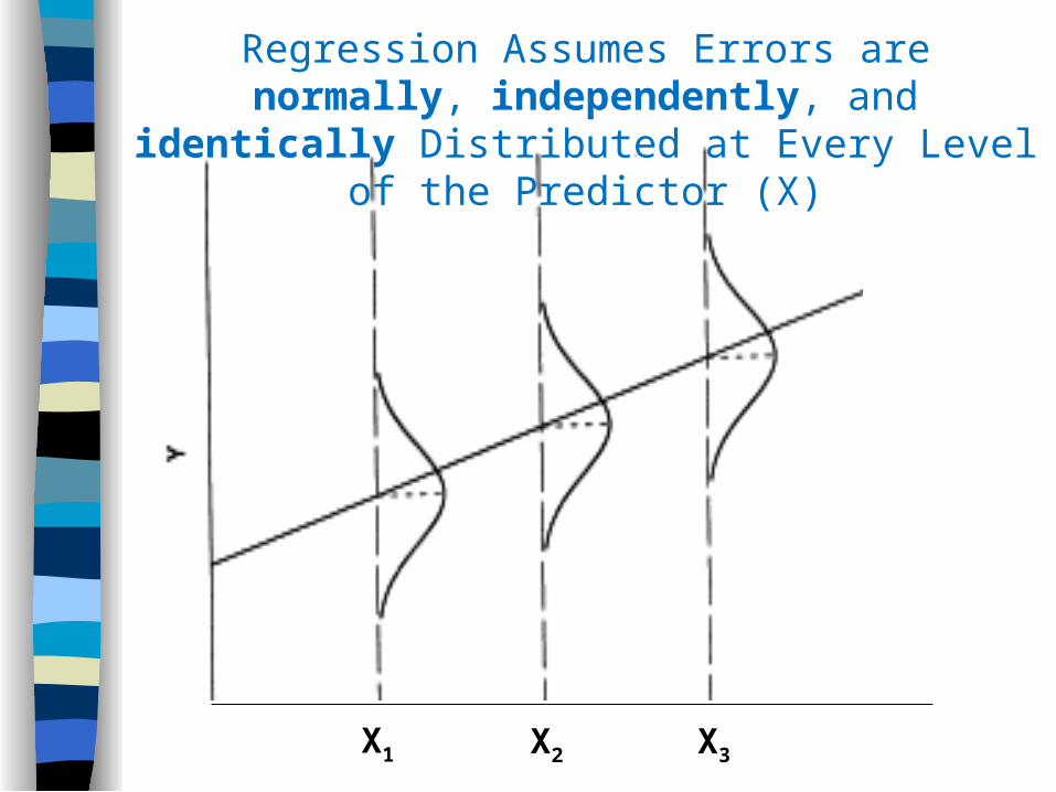
Regression Assumes Errors are normally, independently, and identically Distributed at Every Level of the Predictor (X)

X1 X2 X3

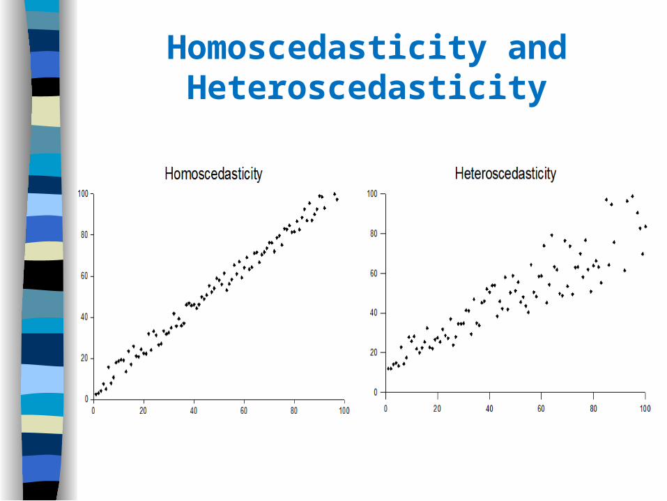
Homoscedasticity and Heteroscedasticity

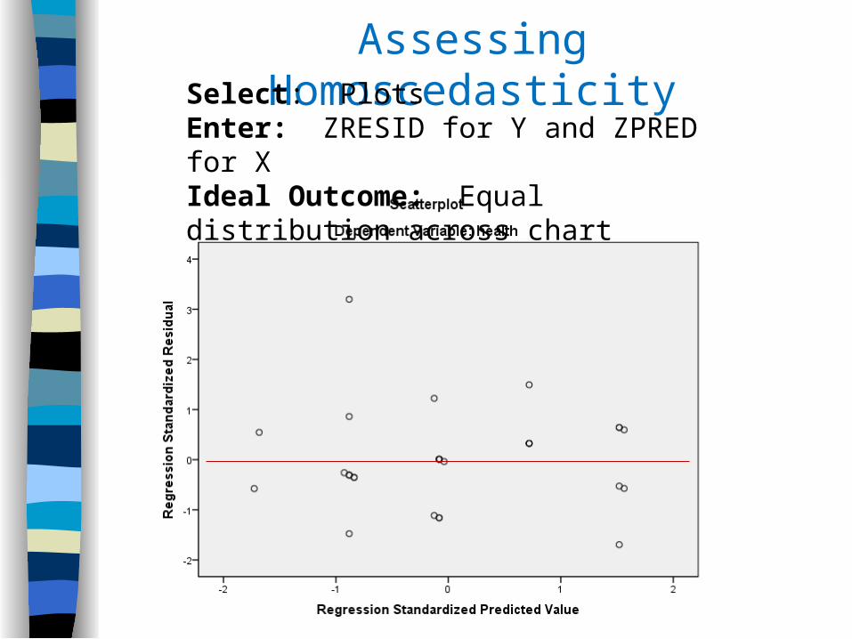
Assessing HomoscedasticitySelect: Plots Enter: ZRESID for Y and ZPRED for XIdeal Outcome: Equal distribution across chart

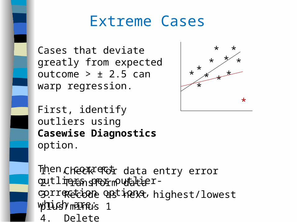
Extreme Cases

*

**

*

** **

**

*

*Cases that deviate greatly from expected outcome > ± 2.5 can warp regression.

First, identify outliers using Casewise Diagnostics option.

Then, correct outliers per outlier-correction options, which are:

1. Check for data entry error2. Transform data 3. Recode as next highest/lowest plus/minus 14. Delete

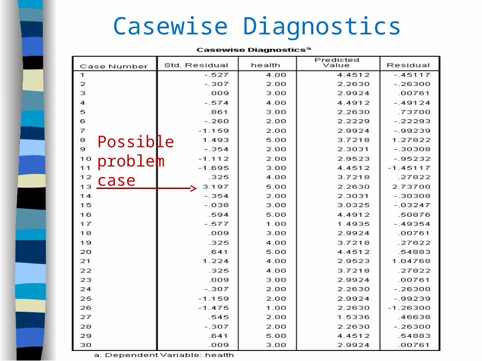
Casewise Diagnostics Print-out in SPSS

Possible problem case

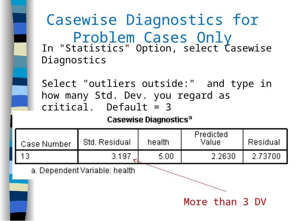
Casewise Diagnostics for Problem Cases Only

In "Statistics" Option, select Casewise Diagnostics

Select "outliers outside:" and type in how many Std. Dev. you regard as critical. Default = 3

More than 3 DV

What If Assumption(s) are Violated?

What is problem with violating assumptions?

Can't generalize obtained model from test sample to wider population.

Overall, not much can be done if assumptions are substantially violated (i.e., extreme heteroscedasticity, extreme auto-correlation, severe non-linearity).

Some options:

1. Heteroscedasticity: Transform raw data (sqr. root, etc.)2. Non-linearity: Attempt logistic regression

A Word About Regression Assumptions and Diagnostics

Are these conditions complicated to understand? Yes

Are they laborious to check and correct? Yes

Do most researchers understand, monitor, and address these conditions? No

Even journal reviewers are often unschooled, or don’t take time, to check diagnostics. Journal space discourages authors from discussing diagnostics. Some have called for more attention to this inattention, but not much action.

Should we do diagnostics? GIGO, and fundamental ethics.

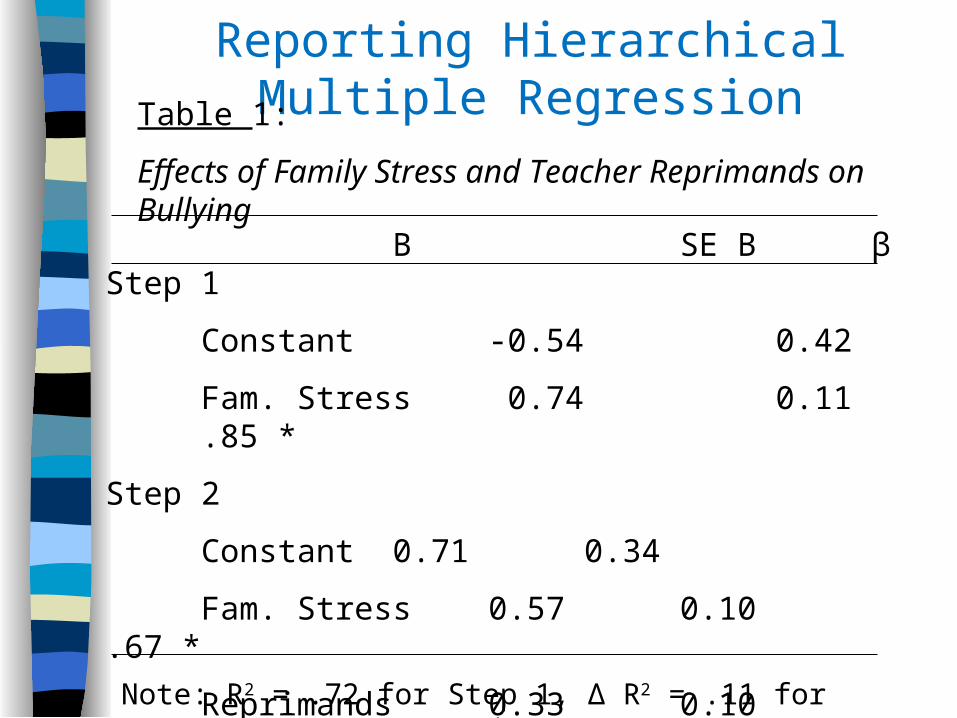
Reporting Hierarchical Multiple Regression

B SE B βStep 1

Constant -0.54 0.42

Fam. Stress 0.74 0.11 .85 *

Step 2

Constant 0.71 0.34

Fam. Stress 0.57 0.10 .67 *

Reprimands 0.33 0.10 .38 *

Table 1:

Effects of Family Stress and Teacher Reprimands on Bullying

Note: R2 = .72 for Step 1, Δ R2 = .11 for Step 2 (p = .004); * p < .01

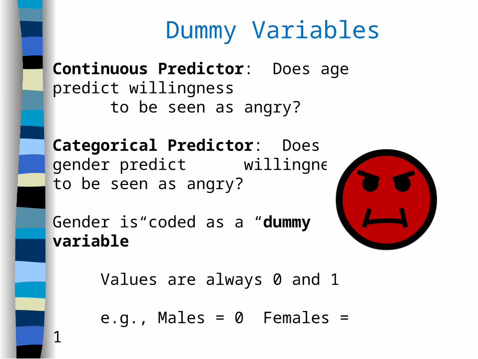
Dummy VariablesContinuous Predictor: Does age predict willingness

to be seen as angry?

Categorical Predictor: Does gender predict willingness to be seen as angry?

Gender is coded as a “dummy variable”

Values are always 0 and 1

e.g., Males = 0 Females = 1

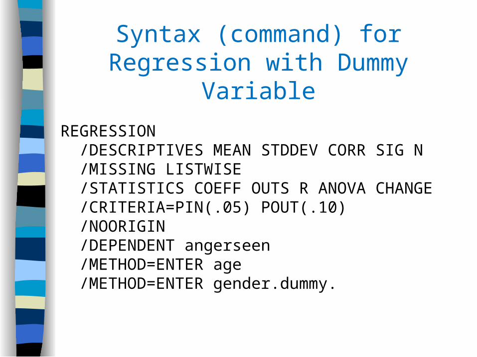
REGRESSION /DESCRIPTIVES MEAN STDDEV CORR SIG N /MISSING LISTWISE /STATISTICS COEFF OUTS R ANOVA CHANGE /CRITERIA=PIN(.05) POUT(.10) /NOORIGIN /DEPENDENT angerseen /METHOD=ENTER age /METHOD=ENTER gender.dummy.

Syntax (command) for Regression with Dummy Variable

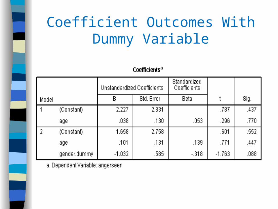
Coefficient Outcomes With Dummy Variable

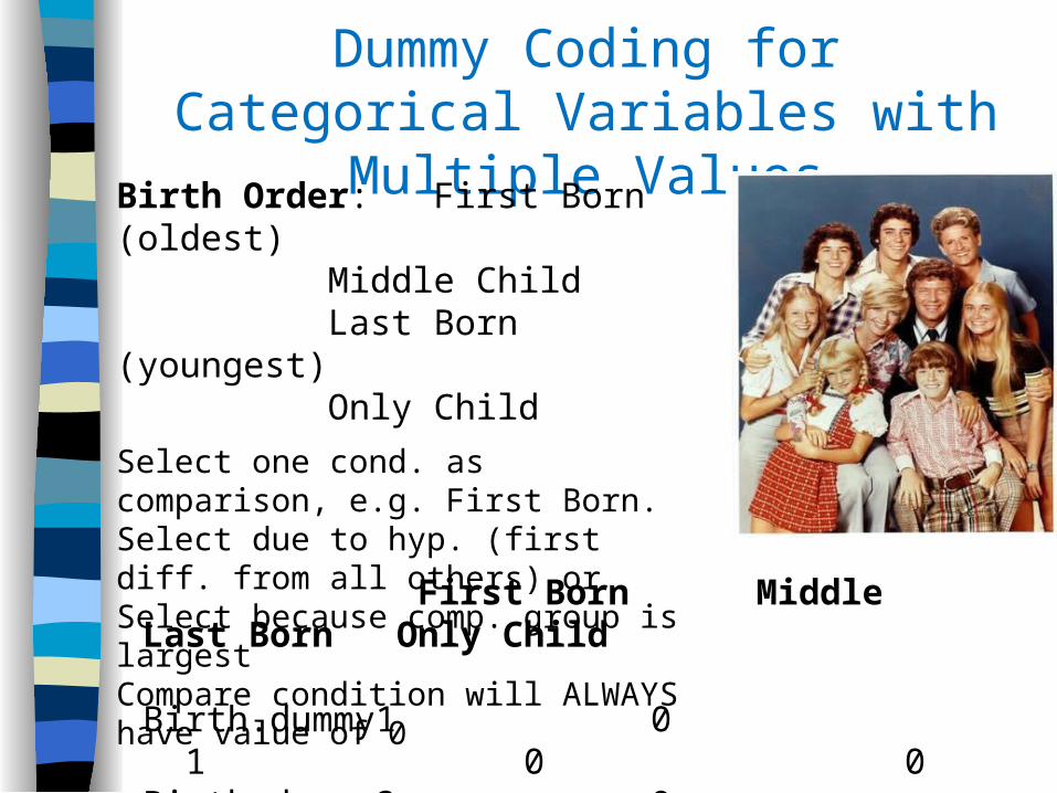
Dummy Coding for Categorical Variables with Multiple Values

Birth Order: First Born (oldest)Middle ChildLast Born (youngest)Only Child

Select one cond. as comparison, e.g. First Born. Select due to hyp. (first diff. from all others) or Select because comp. group is largest Compare condition will ALWAYS have value of 0

First Born Middle Last Born Only Child

Birth.dummy1 0 1 0 0Birth.dummy2 0 0 1 0Birth.dummy3 0 0 0 1

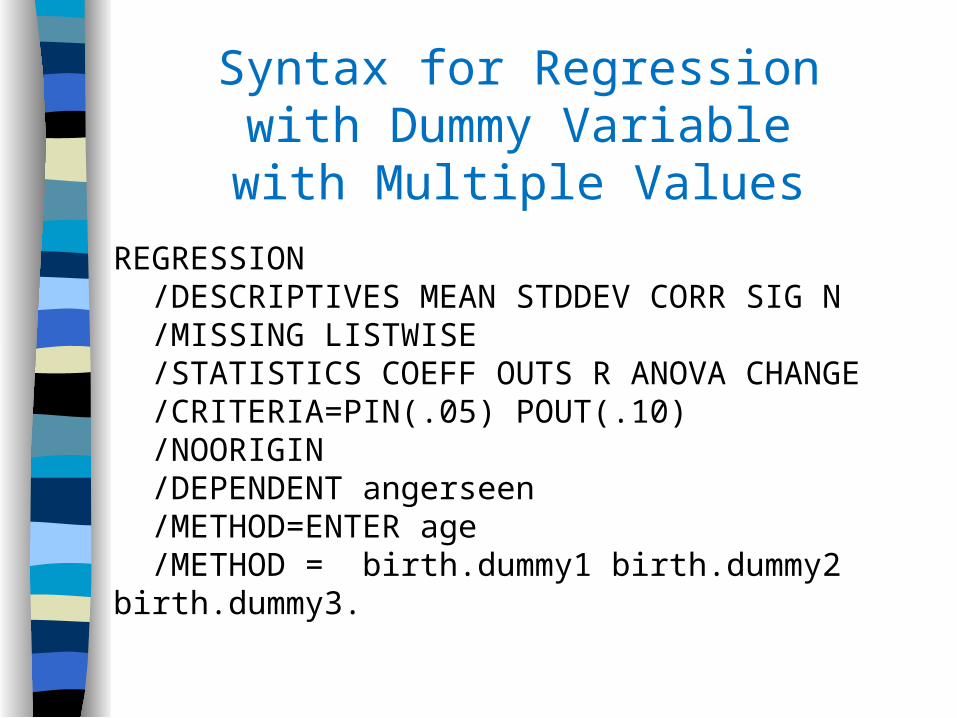
REGRESSION /DESCRIPTIVES MEAN STDDEV CORR SIG N /MISSING LISTWISE /STATISTICS COEFF OUTS R ANOVA CHANGE /CRITERIA=PIN(.05) POUT(.10) /NOORIGIN /DEPENDENT angerseen /METHOD=ENTER age /METHOD = birth.dummy1 birth.dummy2 birth.dummy3.

Syntax for Regression with Dummy Variable with Multiple Values

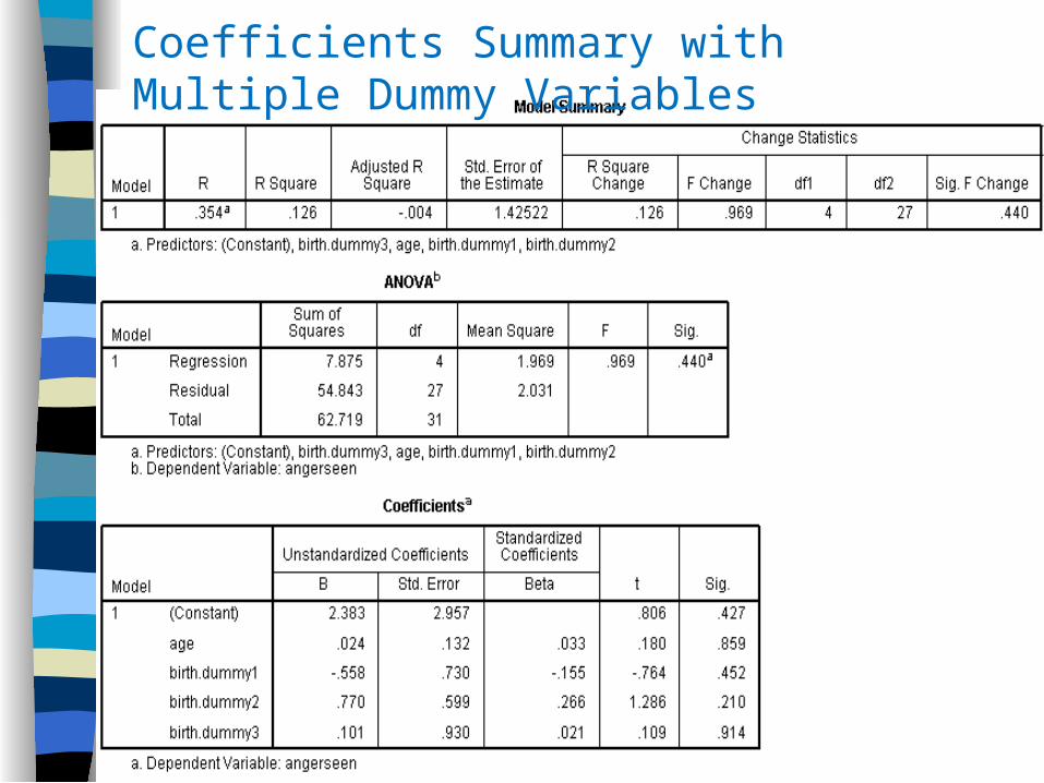
Coefficients Summary with Multiple Dummy Variables

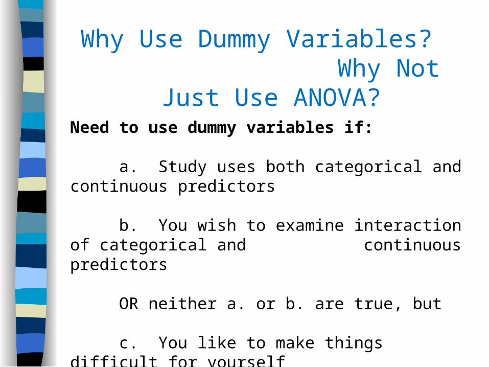
Why Use Dummy Variables? Why Not Just Use ANOVA?

Need to use dummy variables if:

a. Study uses both categorical and continuous predictors

b. You wish to examine interaction of categorical and continuous predictors

OR neither a. or b. are true, but

c. You like to make things difficult for yourself