Embed Size (px)
DESCRIPTION
Multiple Regression. Multiple Regression. The test you choose depends on level of measurement: Independent VariableDependentVariableTest DichotomousInterval-Ratio Independent Samples t-test Dichotomous NominalNominalCross Tabs DichotomousDichotomous - PowerPoint PPT Presentation
Citation preview

Multiple Regression
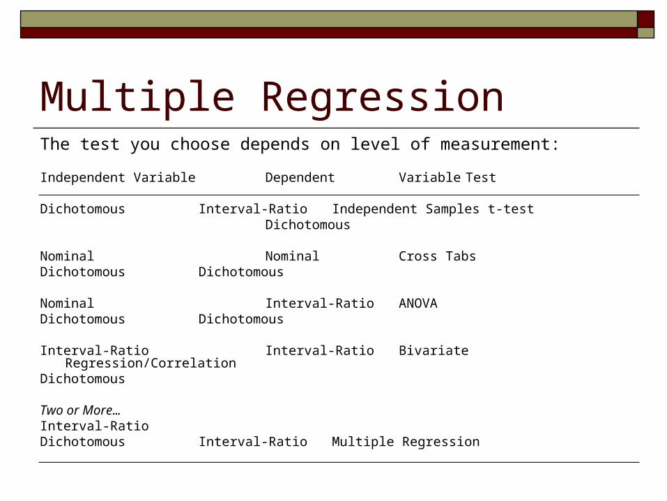
Multiple RegressionThe test you choose depends on level of measurement:
Independent Variable Dependent Variable Test
Dichotomous Interval-Ratio Independent Samples t-testDichotomous
Nominal Nominal Cross TabsDichotomous Dichotomous
Nominal Interval-Ratio ANOVADichotomous Dichotomous
Interval-Ratio Interval-Ratio Bivariate Regression/CorrelationDichotomous
Two or More…Interval-Ratio Dichotomous Interval-Ratio Multiple Regression
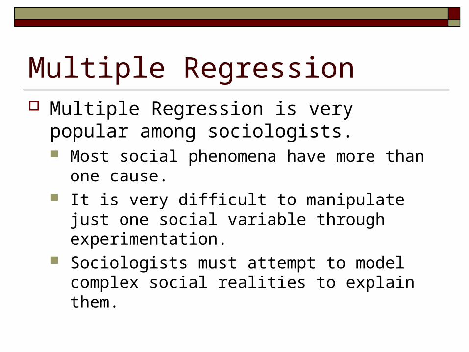
Multiple Regression Multiple Regression is very popular among
sociologists. Most social phenomena have more than one
cause. It is very difficult to manipulate just one social
variable through experimentation. Sociologists must attempt to model complex
social realities to explain them.
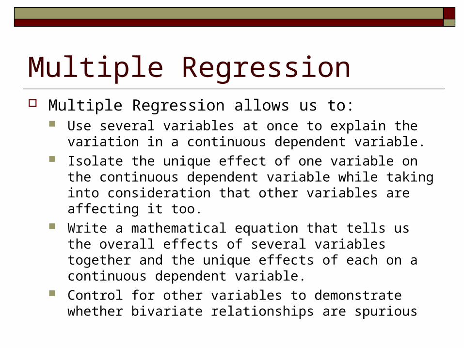
Multiple Regression Multiple Regression allows us to:
Use several variables at once to explain the variation in a continuous dependent variable.
Isolate the unique effect of one variable on the continuous dependent variable while taking into consideration that other variables are affecting it too.
Write a mathematical equation that tells us the overall effects of several variables together and the unique effects of each on a continuous dependent variable.
Control for other variables to demonstrate whether bivariate relationships are spurious
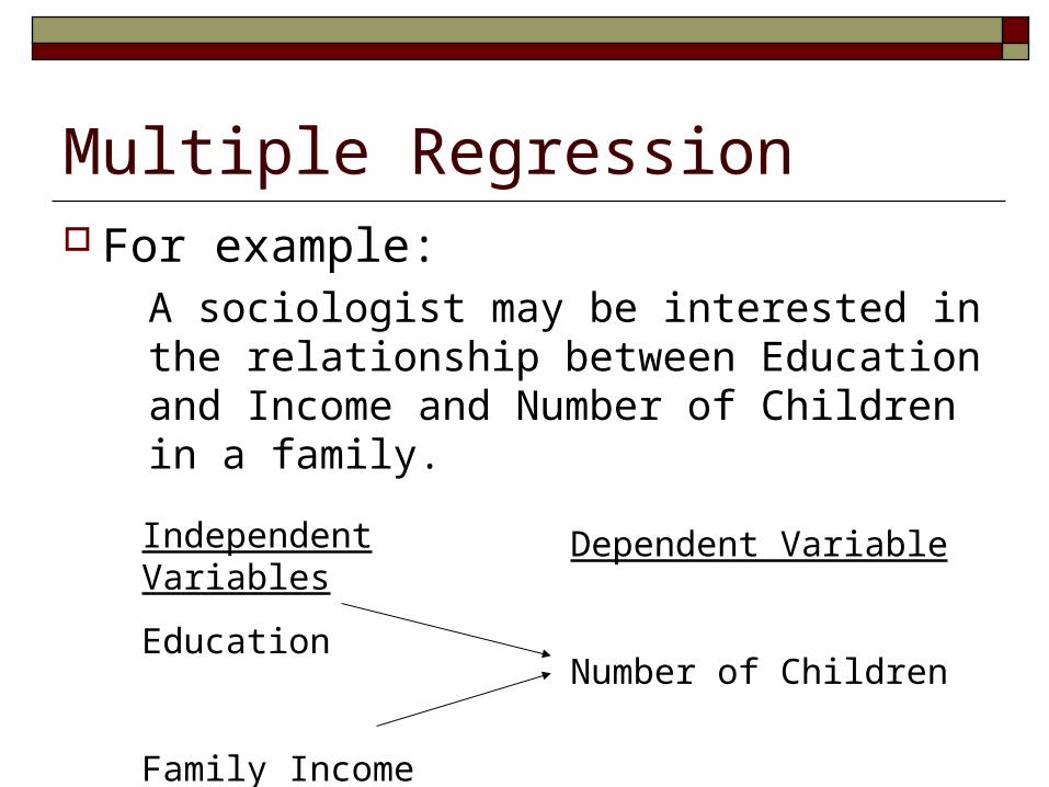
Multiple Regression For example:
A sociologist may be interested in the relationship between Education and Income and Number of Children in a family.
Independent Variables
Education
Family Income
Dependent Variable
Number of Children

Multiple Regression
For example: Null Hypothesis: There is no relationship between
education of respondents and the number of children in families. Ho : b1 = 0
Null Hypothesis: There is no relationship between family income and the number of children in families. Ho : b2 = 0
Independent Variables
Education
Family Income
Dependent Variable
Number of Children

Multiple Regression
Bivariate regression is based on fitting a line as close as possible to the plotted coordinates of your data on a two-dimensional graph.
Trivariate regression is based on fitting a plane as close as possible to the plotted coordinates of your data on a three-dimensional graph.
Case: 1 2 3 4 5 6 7 8 9 10 11 12 13 14 15 16 17 18 19 20 21 22 23 24 25
Children (Y): 2 5 1 9 6 3 0 3 7 7 2 5 1 9 6 3 0 3 7 14 2 5 1 9 6
Education (X1) 12 16 2012 9 18 16 14 9 12 12 10 20 11 9 18 16 14 9 8 12 10 20 11 9
Income 1=$10K (X2): 3 4 9 5 4 12 10 1 4 3 10 4 9 4 4 12 10 6 4 1 10 3 9 2 4

Multiple Regression
Case: 1 2 3 4 5 6 7 8 9 10 11 12 13 14 15 16 17 18 19 20 21 22 23 24 25
Children (Y): 2 5 1 9 6 3 0 3 7 7 2 5 1 9 6 3 0 3 7 14 2 5 1 9 6
Education (X1) 12 16 2012 9 18 16 14 9 12 12 10 20 11 9 18 16 14 9 8 12 10 20 11 9
Income 1=$10K (X2): 3 4 9 5 4 12 10 1 4 3 10 4 9 4 4 12 10 6 4 1 10 3 9 2 4
Y
X1X2
0
Plotted coordinates (1 – 10) for Education, Income and Number of Children
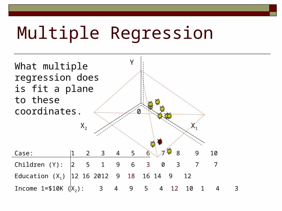
Multiple Regression
Case: 1 2 3 4 5 6 7 8 9 10
Children (Y): 2 5 1 9 6 3 0 3 7 7
Education (X1) 12 16 2012 9 18 16 14 9 12
Income 1=$10K (X2): 3 4 9 5 4 12 10 1 4 3
Y
X1X2
0
What multiple regression does is fit a plane to these coordinates.

Multiple Regression Mathematically, that plane is:
Y = a + b1X1 + b2X2
a = y-intercept, where X’s equal zero
b=coefficient or slope for each variable
For our problem, SPSS says the equation is:
Y = 11.8 - .36X1 - .40X2
Expected # of Children = 11.8 - .36*Educ - .40*Income
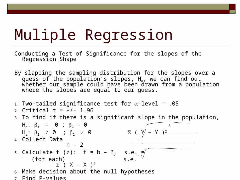
Muliple RegressionConducting a Test of Significance for the slopes of the Regression Shape
By slapping the sampling distribution for the slopes over a guess of the population’s slopes, Ho, we can find out whether our sample could have been drawn from a population where the slopes are equal to our guess.
1. Two-tailed significance test for -level = .052. Critical t = +/- 1.963. To find if there is a significant slope in the population,
Ho: 1 = 0 ; 2 = 0Ha: 1 0 ; 2 0 ( Y – Y )2
4. Collect Data n - 25. Calculate t (z): t = b – o s.e. = (for each) s.e. ( X – X )2
6. Make decision about the null hypotheses7. Find P-values

Multiple RegressionModel Summary
.757a .573 .534 2.33785Model1
R R SquareAdjustedR Square
Std. Error ofthe Estimate
Predictors: (Constant), Income, Educationa. ANOVAb
161.518 2 80.759 14.776 .000a
120.242 22 5.466
281.760 24
Regression
Residual
Total
Model1
Sum ofSquares df Mean Square F Sig.
Predictors: (Constant), Income, Educationa.
Dependent Variable: Childrenb.
Coefficientsa
11.770 1.734 6.787 .000
-.364 .173 -.412 -2.105 .047
-.403 .194 -.408 -2.084 .049
(Constant)
Education
Income
Model1
B Std. Error
UnstandardizedCoefficients
Beta
StandardizedCoefficients
t Sig.
Dependent Variable: Childrena.
Y = 11.8 - .36X1 - .40X2
Sig. Tests
t-scores and
P-values

Multiple Regression R2
TSS – SSE / TSS TSS = Distance from mean to value on Y for each case SSE = Distance from shape to value on Y for each case
Can be interpreted the same for multiple regression—joint explanatory value of all of your variables (or “your model”)
Can request a change in R2 test from SPSS to see if adding new variables improves the fit of your model
Model Summary
.757a .573 .534 2.33785Model1
R R SquareAdjustedR Square
Std. Error ofthe Estimate
Predictors: (Constant), Income, Educationa.

Multiple RegressionModel Summary
.757a .573 .534 2.33785Model1
R R SquareAdjustedR Square
Std. Error ofthe Estimate
Predictors: (Constant), Income, Educationa. ANOVAb
161.518 2 80.759 14.776 .000a
120.242 22 5.466
281.760 24
Regression
Residual
Total
Model1
Sum ofSquares df Mean Square F Sig.
Predictors: (Constant), Income, Educationa.
Dependent Variable: Childrenb.
Coefficientsa
11.770 1.734 6.787 .000
-.364 .173 -.412 -2.105 .047
-.403 .194 -.408 -2.084 .049
(Constant)
Education
Income
Model1
B Std. Error
UnstandardizedCoefficients
Beta
StandardizedCoefficients
t Sig.
Dependent Variable: Childrena.
Y = 11.8 - .36X1 - .40X2
57% of the variation in number of children is explained by education and income!

Multiple RegressionModel Summary
.757a .573 .534 2.33785Model1
R R SquareAdjustedR Square
Std. Error ofthe Estimate
Predictors: (Constant), Income, Educationa. ANOVAb
161.518 2 80.759 14.776 .000a
120.242 22 5.466
281.760 24
Regression
Residual
Total
Model1
Sum ofSquares df Mean Square F Sig.
Predictors: (Constant), Income, Educationa.
Dependent Variable: Childrenb.
Coefficientsa
11.770 1.734 6.787 .000
-.364 .173 -.412 -2.105 .047
-.403 .194 -.408 -2.084 .049
(Constant)
Education
Income
Model1
B Std. Error
UnstandardizedCoefficients
Beta
StandardizedCoefficients
t Sig.
Dependent Variable: Childrena.
Y = 11.8 - .36X1 - .40X2
r2
(Y – Y)2 - (Y – Y)2
(Y – Y)2
161.518 ÷ 261.76 = .573

Multiple RegressionSo what does our equation tell us?
Y = 11.8 - .36X1 - .40X2
Expected # of Children = 11.8 - .36*Educ - .40*Income
Try “plugging in” some values for your variables.

Multiple Regression
So what does our equation tell us?
Y = 11.8 - .36X1 - .40X2
Expected # of Children = 11.8 - .36*Educ - .40*Income
If Education equals:& If Income Equals: Then, children equals: 0 0 11.810 0 8.210 10 4.2 20 10 0.620 11 0.2
^

Multiple RegressionSo what does our equation tell us?
Y = 11.8 - .36X1 - .40X2
Expected # of Children = 11.8 - .36*Educ - .40*Income
If Education equals:& If Income Equals: Then, children equals:
1 0 11.44
1 1 11.04
1 5 9.44
1 10 7.44
1 15 5.44
^

Multiple RegressionSo what does our equation tell us?
Y = 11.8 - .36X1 - .40X2
Expected # of Children = 11.8 - .36*Educ - .40*Income
If Education equals:& If Income Equals: Then, children equals:
0 1 11.40
1 1 11.04
5 1 9.60
10 1 7.80
15 1 6.00
^
Multiple Regression
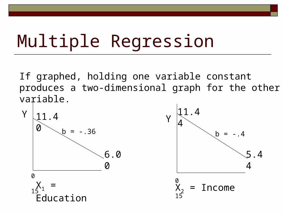
If graphed, holding one variable constant produces a two-dimensional graph for the other variable.
Y
X2 = Income0 15
11.44
5.44
b = -.4
Y
X1 = Education0 15
11.40
6.00
b = -.36

Multiple Regression An interesting effect of controlling for other
variables is “Simpson’s Paradox.” The direction of relationship between two
variables can change when you control for another variable.
Education Crime Rate Y = -51.3 + 1.5X+

Multiple Regression “Simpson’s Paradox”
Education Crime Rate Y = -51.3 + 1.5X1
+
Urbanization (is related to both)
Education
Crime Rate
+
+
Regression Controlling for Urbanization
Education
UrbanizationCrime Rate
-
+Y = 58.9 - .6X1 + .7X2

Multiple Regression
Crime
Education
Original Regression Line
Looking at each level of urbanization, new lines
Rural
Small town
Suburban
City
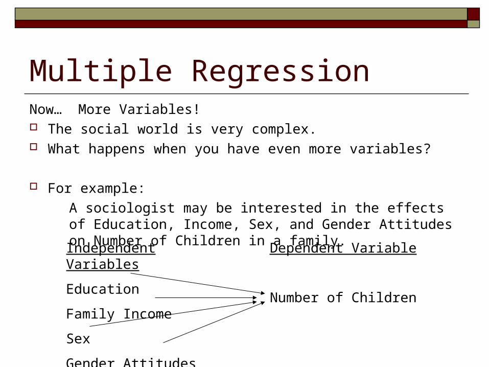
Multiple RegressionNow… More Variables! The social world is very complex. What happens when you have even more variables?
For example:
A sociologist may be interested in the effects of Education, Income, Sex, and Gender Attitudes on Number of Children in a family.
Independent Variables
Education
Family Income
Sex
Gender Attitudes
Dependent Variable
Number of Children

Multiple Regression
Null Hypotheses:1. There will be no relationship between education of respondents and
the number of children in families. Ho : b1 = 0 Ha : b1 ≠ 0
2. There will be no relationship between family income and the number of children in families. Ho : b2 = 0 Ha : b2 ≠ 0
3. There will be no relationship between sex and number of children. Ho: b3 = 0 Ha : b3 ≠ 0
4. There will be no relationship between gender attitudes and number of children. Ho : b4 = 0 Ha : b4 ≠ 0
Independent Variables
Education
Family Income
Sex
Gender Attitudes
Dependent Variable
Number of Children
Multiple Regression
Bivariate regression is based on fitting a line as close as possible to the plotted coordinates of your data on a two-dimensional graph.
Trivariate regression is based on fitting a plane as close as possible to the plotted coordinates of your data on a three-dimensional graph.
Regression with more than two independent variables is based on fitting a shape to your constellation of data on an multi-dimensional graph.
Multiple Regression
Regression with more than two independent variables is based on fitting a shape to your constellation of data on an multi-dimensional graph.
The shape will be placed so that it minimizes the distance (sum of squared errors) from the shape to every data point.

Multiple Regression
Regression with more than two independent variables is based on fitting a shape to your constellation of data on an multi-dimensional graph.
The shape will be placed so that it minimizes the distance (sum of squared errors) from the shape to every data point.
The shape is no longer a line, but if you hold all other variables constant, it is linear for each independent variable.
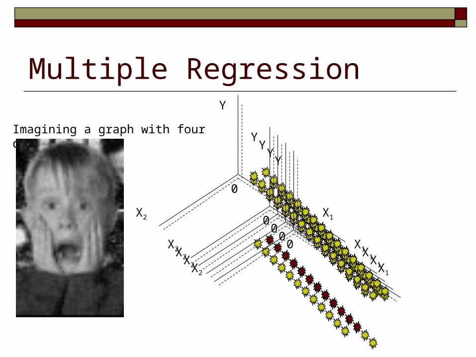
Multiple RegressionY
X1X2
0
Imagining a graph with four dimensions!Y
X1X2
0
Y
X1X2
0
Y
X1X2
0
Y
X1X2
0

Multiple RegressionFor our problem, our equation could be:
Y = 7.5 - .30X1 - .40X2 + 0.5X3 + 0.25X4
E(Children) =
7.5 - .30*Educ - .40*Income + 0.5*Sex + 0.25*Gender Att.

Multiple RegressionSo what does our equation tell us?
Y = 7.5 - .30X1 - .40X2 + 0.5X3 + 0.25X4
E(Children) =
7.5 - .30*Educ - .40*Income + 0.5*Sex + 0.25*Gender Att.
Education: Income: Sex: Gender Att: Children:
10 5 0 0 2.5
10 5 0 5 3.75
10 10 0 5 1.75
10 5 1 0 3.0
10 5 1 5 4.25
^

Multiple Regression
Each variable, holding the other variables constant, has a linear, two-dimensional graph of its relationship with the dependent variable.
Here we hold every other variable constant at “zero.”Y
X2 = Education
Y
X1 = Income0 10 0 10
7.57.5
4.5
3.5
b = -.3b = -.4
Y = 7.5 - .30X1 - .40X2 + 0.5X3 + 0.25X4^

Multiple Regression
Y
X3 = Sex
Y
X4 = Gender Attitudes0 1 0 5
7.5 7.5
8
8.75
Each variable, holding the other variables constant, has a linear, two-dimensional graph of its relationship with the dependent variable.
Here we hold every other variable constant at “zero.”
b = .5
b = .25
Y = 7.5 - .30X1 - .40X2 + 0.5X3 + 0.25X4^
Multiple Regression
Okay, we’re almost through with regression!

Multiple Regression Dummy Variables
They are simply dichotomous variables that are entered into regression. They have 0 – 1 coding where 0 = absence of something and 1 = presence of something. E.g., Female (0=M; 1=F) or Southern (0=Non-Southern; 1=Southern).
What are dummy
variables?!
Multiple Regression
But YOU said we
CAN’T do that!
A nominal variable has no rank or order, rendering the numerical coding scheme useless for regression.
Dummy Variables are especially nice because they allow us to use nominal
variables in regression.
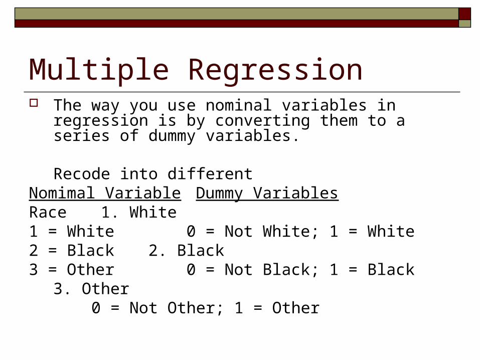
Multiple Regression The way you use nominal variables in regression is by
converting them to a series of dummy variables.
Recode into differentNomimal Variable Dummy VariablesRace 1. White1 = White 0 = Not White; 1 = White2 = Black 2. Black3 = Other 0 = Not Black; 1 = Black
3. Other 0 = Not Other; 1 =
Other

Multiple Regression The way you use nominal variables in regression is by converting them to a
series of dummy variables.Recode into different
Nomimal Variable Dummy VariablesReligion 1. Catholic1 = Catholic 0 = Not Catholic; 1 = Catholic2 = Protestant 2. Protestant3 = Jewish 0 = Not Prot.; 1 = Protestant4 = Muslim 3. Jewish5 = Other Religions 0 = Not Jewish; 1 = Jewish
4. Muslim 0 = Not Muslim; 1 = Muslim5. Other Religions 0 = Not Other; 1 = Other
Relig.
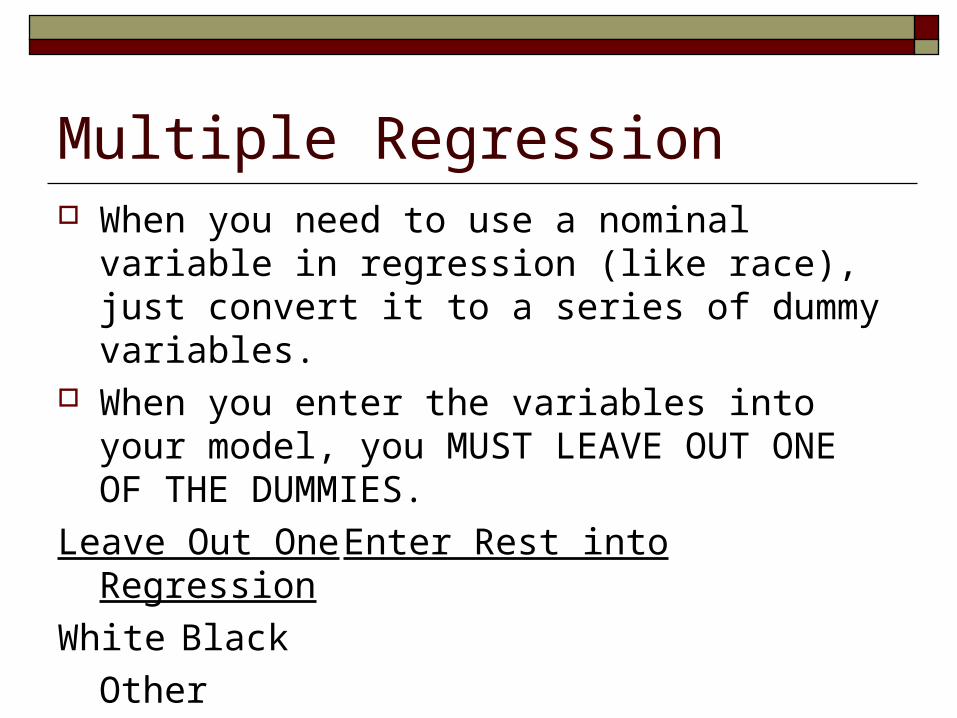
Multiple Regression When you need to use a nominal variable in
regression (like race), just convert it to a series of dummy variables.
When you enter the variables into your model, you MUST LEAVE OUT ONE OF THE DUMMIES.
Leave Out One Enter Rest into Regression
White Black
Other

Multiple Regression The reason you MUST LEAVE OUT ONE OF THE
DUMMIES is that regression is mathematically impossible without an excluded group.
If all were in, holding one of them constant would prohibit variation in all the rest.
Leave Out One Enter Rest into Regression
Catholic Protestant
Jewish
Muslim
Other Religion

Multiple Regression The regression equations for dummies will
look the same.For Race, with 3 dummies, predicting self-esteem:
Y = a + b1X1 + b2X2
a = the y-intercept, which in this case is the predicted value of self-esteem for the excluded group, white.
b1 = the slope for variable X1, black
b2 = the slope for variable X2, other

Multiple Regression If our equation were:For Race, with 3 dummies, predicting self-esteem:
Y = 28 + 5X1 – 2X2
a = the y-intercept, which in this case is the predicted value of self-esteem for the excluded group, white.
5 = the slope for variable X1, black
-2 = the slope for variable X2, other
Plugging in values for the dummies tells you each group’s self-esteem average:
White = 28
Black = 33
Other = 26
When cases’ values for X1 = 0 and X2 = 0, they are white;
when X1 = 1 and X2 = 0, they are black;
when X1 = 0 and X2 = 1, they are other.
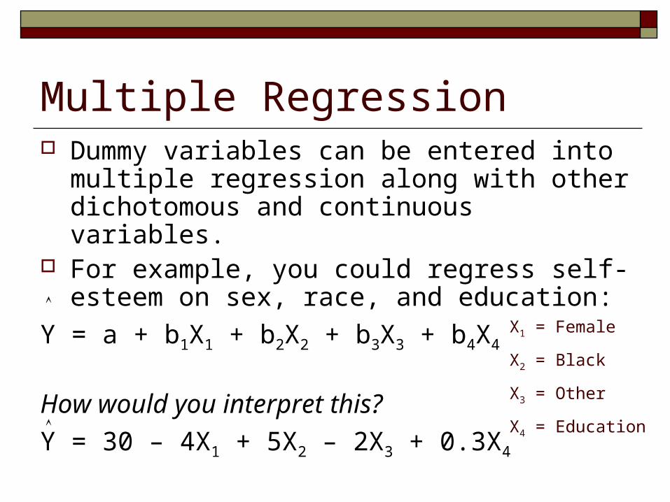
Multiple Regression Dummy variables can be entered into multiple
regression along with other dichotomous and continuous variables.
For example, you could regress self-esteem on sex, race, and education:
Y = a + b1X1 + b2X2 + b3X3 + b4X4
How would you interpret this?
Y = 30 – 4X1 + 5X2 – 2X3 + 0.3X4
X1 = Female
X2 = Black
X3 = Other
X4 = Education
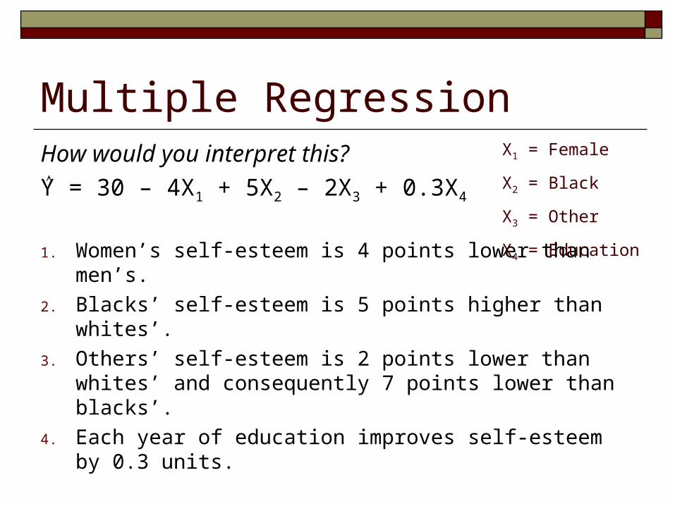
Multiple RegressionHow would you interpret this?
Y = 30 – 4X1 + 5X2 – 2X3 + 0.3X4
1. Women’s self-esteem is 4 points lower than men’s.
2. Blacks’ self-esteem is 5 points higher than whites’.
3. Others’ self-esteem is 2 points lower than whites’ and consequently 7 points lower than blacks’.
4. Each year of education improves self-esteem by 0.3 units.
X1 = Female
X2 = Black
X3 = Other
X4 = Education

Multiple RegressionHow would you interpret this?
Y = 30 – 4X1 + 5X2 – 2X3 + 0.3X4
Plugging in some select values, we’d get self-esteem for select groups:
White males with 10 years of education = 33 Black males with 10 years of education = 38 Other females with 10 years of education = 27 Other females with 16 years of education = 28.8
X1 = Female
X2 = Black
X3 = Other
X4 = Education
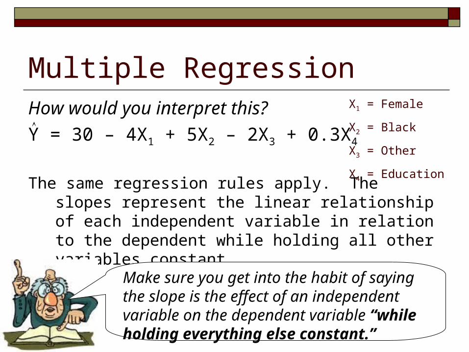
Multiple RegressionHow would you interpret this?
Y = 30 – 4X1 + 5X2 – 2X3 + 0.3X4
The same regression rules apply. The slopes represent the linear relationship of each independent variable in relation to the dependent while holding all other variables constant.
X1 = Female
X2 = Black
X3 = Other
X4 = Education
Make sure you get into the habit of saying the slope is the effect of an independent variable on the dependent variable “while holding everything else constant.”

Multiple RegressionStandardized Coefficients Sometimes you want to know whether one variable has
a larger impact on your dependent variable than another.
If your variables have different units of measure, it is hard to compare their effects.
For example, if wages go up one thousand dollars for each year of education, is that a greater effect than if wages go up five hundred dollars for each year increase in age.

Multiple RegressionStandardized Coefficients So which is better for increasing wages, education or aging? One thing you can do is “standardize” your slopes so that
you can compare the standard deviation increase in your dependent variable for each standard deviation increase in your independent variables.
You might find that Wages go up 0.3 standard deviations for each standard deviation increase in education, but 0.4 standard deviations for each standard deviation increase in age.

Multiple RegressionStandardized Coefficients Recall that standardizing regression coefficients is accomplished
by the formula: b(Sx/Sy)
In the example above, education and income have very comparable effects on number of children.
Each lowers the number of children by .4 standard deviations for a standard deviation increase in each, controlling for the other.
Coefficientsa
11.770 1.734 6.787 .000
-.364 .173 -.412 -2.105 .047
-.403 .194 -.408 -2.084 .049
(Constant)
Education
Income
Model1
B Std. Error
UnstandardizedCoefficients
Beta
StandardizedCoefficients
t Sig.
Dependent Variable: Childrena.

Multiple RegressionStandardized Coefficients One last note of caution...
It does not make sense to standardize slopes for dichotomous variables.
It makes no sense to refer to standard deviation increases in sex, or in race--these are either 0 or they are 1 only.
Multiple Regression
Give yourself a hand…
You now understand more statistics that 99% of the population!
You are well-qualified for understanding most sociological research papers.