Multiple random variables, Correlations

Multiple random variables,Correlations

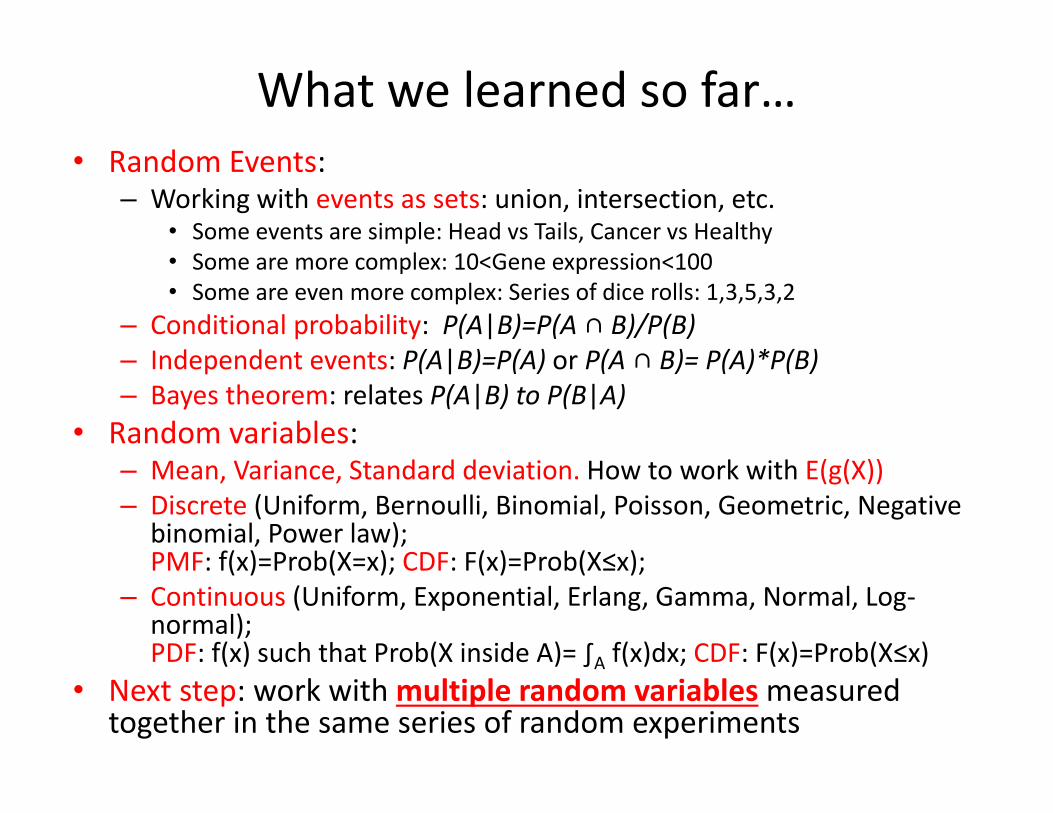
What we learned so far…• Random Events:

– Working with events as sets: union, intersection, etc.• Some events are simple: Head vs Tails, Cancer vs Healthy• Some are more complex: 10<Gene expression<100• Some are even more complex: Series of dice rolls: 1,3,5,3,2

– Conditional probability: P(A|B)=P(A ∩ B)/P(B)– Independent events: P(A|B)=P(A) or P(A ∩ B)= P(A)*P(B)– Bayes theorem: relates P(A|B) to P(B|A)

• Random variables:– Mean, Variance, Standard deviation. How to work with E(g(X))– Discrete (Uniform, Bernoulli, Binomial, Poisson, Geometric, Negative

binomial, Power law); PMF: f(x)=Prob(X=x); CDF: F(x)=Prob(X≤x);

– Continuous (Uniform, Exponential, Erlang, Gamma, Normal, Log‐normal);PDF: f(x) such that Prob(X inside A)= ∫A f(x)dx; CDF: F(x)=Prob(X≤x)

• Next step: work with multiple random variablesmeasured together in the same series of random experiments

Concept of Joint Probabilities

• Biological systems are usually described not by a single random variable but by many random variables

• Example: The expression state of a human cell: 20,000 random variables Xi for each of its genes

• A joint probability distribution describes the behavior of several random variables

• We will start with just two random variables X and Y and generalize when necessary

Chapter 5 Introduction 3

Joint Probability Mass Function Defined

Sec 5‐1.1 Joint Probability Distributions 4

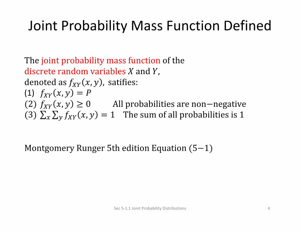
The joint probability mass function of the discrete random variables 𝑋 and 𝑌, denoted as 𝑓 𝑥,𝑦 , satifies:(1) 𝑓 𝑥,𝑦 𝑃2 𝑓 𝑥,𝑦 0 All probabilities are non negative3 ∑ ∑ 𝑓 𝑥,𝑦 1 The sum of all probabilities is 1

Montgomery Runger 5th edition Equation 5 1

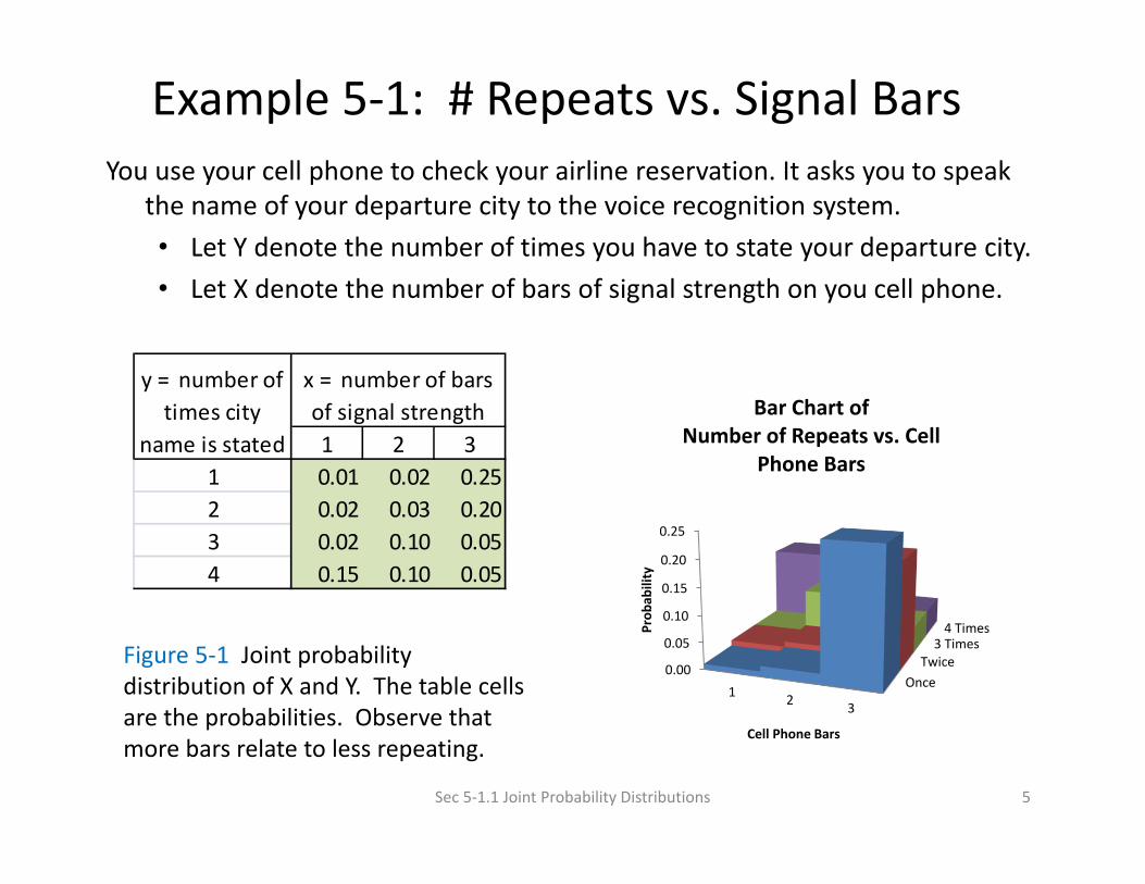
Example 5‐1: # Repeats vs. Signal BarsYou use your cell phone to check your airline reservation. It asks you to speak

the name of your departure city to the voice recognition system.• Let Y denote the number of times you have to state your departure city.• Let X denote the number of bars of signal strength on you cell phone.


Figure 5‐1 Joint probability distribution of X and Y. The table cells are the probabilities. Observe that more bars relate to less repeating.

OnceTwice3 Times4 Times

0.00

0.05

0.10

0.15

0.20

0.25

1 2 3

Prob

ability

Cell Phone Bars

Bar Chart of Number of Repeats vs. Cell

Phone Bars1 2 3

1 0.01 0.02 0.252 0.02 0.03 0.203 0.02 0.10 0.054 0.15 0.10 0.05

x = number of bars of signal strength

y = number of times city

name is stated

Marginal Probability Distributions (discrete)For a discrete joint PDF, there are marginal distributions for each random variable, formed by summing the joint PMF over the other variable.

Sec 5‐1.2 Marginal Probability Distributions 6

𝑓 𝑥 𝑓 𝑥, 𝑦

𝑓 𝑦 𝑓 𝑥, 𝑦

1 2 3 f Y (y ) =1 0.01 0.02 0.25 0.282 0.02 0.03 0.20 0.253 0.02 0.10 0.05 0.174 0.15 0.10 0.05 0.30f X (x ) = 0.20 0.25 0.55 1.00


y = number of times city name

is stated

Figure 5‐6 From the prior example, the joint PMF is shown in green while the two marginal PMFs are shown in purple.

Called marginal because they are written in the margins

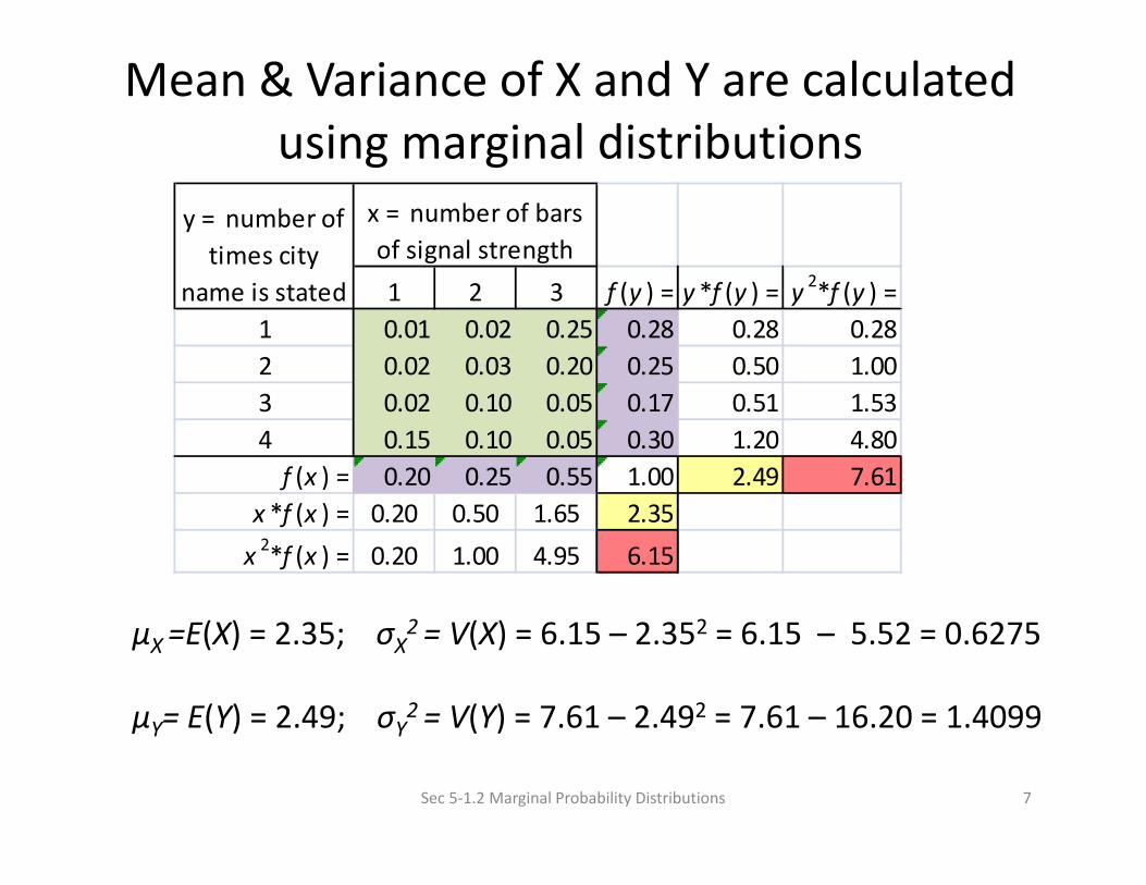
Mean & Variance of X and Y are calculated using marginal distributions


1 2 3 f (y ) = y *f (y ) = y 2*f (y ) =1 0.01 0.02 0.25 0.28 0.28 0.282 0.02 0.03 0.20 0.25 0.50 1.003 0.02 0.10 0.05 0.17 0.51 1.534 0.15 0.10 0.05 0.30 1.20 4.80f (x ) = 0.20 0.25 0.55 1.00 2.49 7.61

x *f (x ) = 0.20 0.50 1.65 2.35x 2*f (x ) = 0.20 1.00 4.95 6.15


y = number of times city

name is stated

μX =E(X) = 2.35; σX2 = V(X) = 6.15 – 2.352 = 6.15 – 5.52 = 0.6275

μY= E(Y) = 2.49; σY2 = V(Y) = 7.61 – 2.492 = 7.61 – 16.20 = 1.4099

Conditional Probability Distributions

From Example 5‐1P(Y=1|X=3) = 0.25/0.55 = 0.455P(Y=2|X=3) = 0.20/0.55 = 0.364P(Y=3|X=3) = 0.05/0.55 = 0.091P(Y=4|X=3) = 0.05/0.55 = 0.091

Sum = 1.00

Sec 5‐1.3 Conditional Probability Distributions 8

Recall that 𝑃 𝐵|𝐴𝑃 𝐴 ∩ 𝐵𝑃 𝐴

1 2 3 f Y (y ) =1 0.01 0.02 0.25 0.282 0.02 0.03 0.20 0.253 0.02 0.10 0.05 0.174 0.15 0.10 0.05 0.30f X (x ) = 0.20 0.25 0.55 1.00


y = number of times city name

is stated

Note that there are 12 probabilities conditional on X, and 12 more probabilities conditional upon Y.

P(Y=y|X=x)=P(X=x,Y=y)/P(X=x)==f(x,y)/fX(x)

Joint Random Variable Independence• Random variable independence means that knowledge of the value of X does not change any of the probabilities associated with the values of Y.

• Opposite: Dependence implies that the values of X are influenced by the values of Y

Sec 5‐1.4 Independence 9

Independence for Discrete Random Variables

• Remember independence of events (slide 13 lecture 4) : Events are independent if any one of the three conditions are met:1) P(A|B)=P(A ∩ B)/P(B)=P(A) or 2) P(B|A)= P(A ∩ B)/P(A)=P(B) or 3) P(A ∩ B)=P(A) ∙ P(B)

• Random variables independent if all eventsA that Y=y and B that X=x are independent if any one of these conditions is met:1) P(Y=y|X=x)=P(Y=y) for any x or 2) P(X=x|Y=y)=P(X=x) for any y or 3) P(X=x, Y=y)=P(X=x)∙P(Y=y) for every pair x and y

11

X and Y are Bernoulli variables

What is the marginal PY(Y=0)?A. 1/6B. 2/6C. 3/6D. 4/6E. I don’t know

Get your i‐clickers

Y=0 Y=1X=0 2/6 1/6X=1 2/6 1/6

12


What is the conditional P(X=0|Y=1)?A. 2/6B. 1/2C. 1/6D. 4/6E. I don’t know


Y=0 Y=1X=0 2/6 1/6X=1 2/6 1/6

13


Are they independent?A. yesB. noC. I don’t know


Y=0 Y=1X=0 2/6 1/6X=1 2/6 1/6

14


Are they independent?A. yesB. noC. I don’t know


Y=0 Y=1X=0 1/2 0X=1 0 1/2

Credit: XKCD comics

Joint Probability Density Function Defined


1 𝑓 𝑥, 𝑦 0 for all 𝑥, 𝑦

2 𝑓 𝑥, 𝑦 𝑑𝑥𝑑𝑦 1

3 𝑃 𝑋,𝑌 ⊂ 𝑅 𝑓 𝑥, 𝑦 𝑑𝑥𝑑𝑦 5 2

Figure 5‐2 Joint probability density function for the random variables X and Y. Probability that (X, Y) is in the region R is determined by the volume of fXY(x,y) over the region R.

The joint probability density function for the continuous random variables X and Y, denotes as fXY(x,y), satisfies the following properties:

Joint Probability Density Function Graph


Figure 5‐3 Joint probability density function for the continuous random variables X and Y of expression levels of two different genes. Note the asymmetric, narrow ridge shape of the PDF – indicating that small values in the X dimension are more likely to occur when small values in the Y dimension occur.

Marginal Probability Distributions (continuous)

• Rather than summing a discrete joint PMF, we integrate a continuous joint PDF.

• The marginal PDFs are used to make probability statements about one variable.

• If the joint probability density function of random variables X and Y is fXY(x,y), the marginal probability density functions of X and Y are:


𝑓 𝑥 𝑓 𝑥, 𝑦 𝑑𝑦

𝑓 𝑦 𝑓 𝑥, 𝑦 𝑑𝑥 5 3

𝑓 𝑥 𝑓 𝑥, 𝑦

𝑓 𝑦 𝑓 𝑥,𝑦

Conditional Probability Density Function Defined

Sec 5‐1.3 Conditional Probability Distributions 19

Given continuous random variables 𝑋 and 𝑌 with joint probability density function 𝑓 𝑥, 𝑦 , the conditional probability densiy function of 𝑌 given 𝑋 x is

𝑓 | 𝑦𝑓 𝑥, 𝑦𝑓 𝑥

𝑓 𝑥, 𝑦𝑓 𝑥, 𝑦 𝑑𝑦

if 𝑓 𝑥 0 5 4

which satifies the following properties:1 𝑓 | 𝑦 0

2 𝑓 | 𝑦 𝑑𝑦 1

3 𝑃 𝑌 ⊂ 𝐵|𝑋 𝑥 𝑓 | 𝑦 𝑑𝑦 for any set B in the range of Y

Compare to discrete: P(Y=y|X=x)=fXY(x,y)/fX(x)

Conditional Probability Distributions

• Conditional probability distributions can be developed for multiple random variables by extension of the ideas used for two random variables.

• Suppose p = 5 and we wish to find the distribution of X1, X2 and X3 conditional on X4=x4 and X5=x5.

Sec 5‐1.5 More Than Two Random Variables 20

𝑓 𝑥 , 𝑥 , 𝑥𝑓 𝑥 , 𝑥 , 𝑥 , 𝑥 , 𝑥

𝑓 𝑥 , 𝑥for 𝑓 𝑥 , 𝑥 0.

Independence for Continuous Random Variables

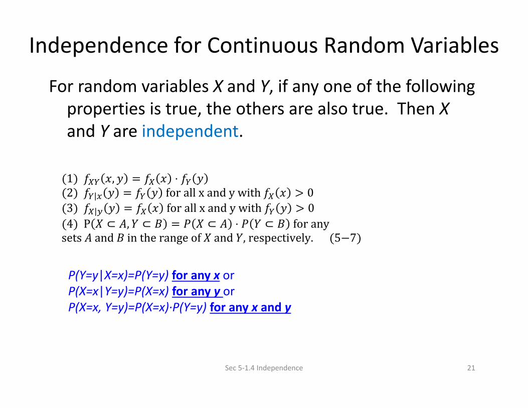
For random variables X and Y, if any one of the following properties is true, the others are also true. Then Xand Y are independent.

Sec 5‐1.4 Independence 21

1 𝑓 𝑥, 𝑦 𝑓 𝑥 ⋅ 𝑓 𝑦2 𝑓 | 𝑦 𝑓 𝑦 for all x and y with 𝑓 𝑥 03 𝑓 | 𝑦 𝑓 𝑥 for all x and y with 𝑓 𝑦 04 P 𝑋 ⊂ 𝐴,𝑌 ⊂ 𝐵 𝑃 𝑋 ⊂ 𝐴 ⋅ 𝑃 𝑌 ⊂ 𝐵 for any

sets 𝐴 and 𝐵 in the range of 𝑋 and 𝑌, respectively. 5 7

P(Y=y|X=x)=P(Y=y) for any x or P(X=x|Y=y)=P(X=x) for any y or P(X=x, Y=y)=P(X=x)∙P(Y=y) for any x and y

26

X and Y are uniformly distributed in the disc x2+y2≤1

Are they independent?

A. yesB. noC. I could not figure it out


Credit: XKCD comics

Documents

Multiple random variables, Correlations