Multiple Model Predictive Control of Dissipative PDE Systems

1206 IEEE TRANSACTIONS ON CONTROL SYSTEMS TECHNOLOGY, VOL. 22, NO. 3, MAY 2014

Multiple Model Predictive Control of Dissipative PDE SystemsIoannis Bonis, Weiguo Xie, and Constantinos Theodoropoulos

Abstract— Model predictive control (MPC) is a popular strat-egy, often applied to distributed parameter systems (DPSs). MostDPSs are approximated by nonlinear large-scale models. Usingit directly for control applications is problematic because ofthe high associated computational cost and the nonconvexityof the underlying optimization problem. In this brief, we buildon the notion of multiple MPC, combining it with equation-free model reduction techniques, to identify the (relativelylow-dimensional) subspace of slow modes and obtain a localreduced-order linear model. This procedure results in aninput/output framework, enabling the use of black-box determin-istic and stochastic simulators. The set of linear low-dimensionalmodels obtained off-line along the reference trajectories are usedfor linear MPC, either with off-line gain scheduling or with onlineidentification of the reduced model. In the former approach, thedecision to use the model in real time is taken a priori, whereasin the latter a local model is computed online as a function ofa set stored in a model bank. The two approaches are discussedand validated using case studies based on a tubular reactor, ahighly nonlinear dissipative partial differential equation systemexhibiting instabilities and multiplicity of state.

Index Terms— Equation-free model reduction, input/outputsimulators, nonlinear partial differential equations (PDEs),trajectory piecewise linearization.

I. INTRODUCTION

CONTROL of distributed parameter systems (DPSs) isa nontrivial task and has received significant attention.

To this end, various approaches are followed: system iden-tification [1], model reduction (nonlinear [2], [3] or linear[4]–[6]), as well as Lyapunov-based approaches [7]. Modelpredictive control is often a strategy of choice for DPS. Boththe linear and nonlinear formulations can be used and both ofthem have shortcomings [8]. To resolve the latter, multiplemodel predictive control is proposed, where the nonlinearmodel is approximated by a set of linear ones for differentregions of operation [9].

In this brief, we present two methodologies tacklingwith the problem of online control of DPS simulated usingdetailed models. Such problems arise naturally when referencetracking is desirable for complex systems. Approximations by

Manuscript received May 5, 2012; revised May 24, 2013; accepted May 31,2013. Manuscript received in final form June 18, 2013. Date of publicationJuly 23, 2013; date of current version April 17, 2014. This work was supportedin part by the European Commission Projects CAFÉ under Grant KBBE-2007-2-01 and CONNECT under Grant COOP-CT-2006-31638. Recommended byAssociate Editor E. Kerrigan.

I. Bonis and C. Theodoropoulos are with the School of Chem-ical Engineering and Analytical Science, University of Manchester,Manchester M13 9PL, U.K. (e-mail: [email protected];[email protected]).

W. Xie was with the School of Chemical Engineering and Analytical Sci-ence, University of Manchester, Manchester M13 9PL, U.K. He is now withthe School of Chemical Engineering, University of Queensland, Brisbane4072, Australia (e-mail: [email protected]).

Color versions of one or more of the figures in this paper are availableonline at http://ieeexplore.ieee.org.

Digital Object Identifier 10.1109/TCST.2013.2270182

(linear or nonlinear) surrogate models usually have a limitedregion of applicability and are deemed insufficient. Thus,there is a strong motivation to use a suitable simulator tocapture the dynamic characteristics of a detailed model forreal-time control.

The controller synthesis framework presented here isdesigned for dissipative systems [7]. Dissipativity is mani-fested as a separation of scales. There is a relatively smallnumber of slow modes, on which the fast ones becomeenslaved after a relatively small time. This is further elucidatedas a spectral gap separating the bulk of the eigenvalues of thesystem from the few dominant ones. The proposed frameworkbuilds on existing accurate models of dissipative systems,solved with black-box simulators. Although such models aretypically partial differential equation (PDE)-based, the algo-rithms presented are even applicable to microscopic/stochasticsystems (e.g., heterogeneous catalytic systems, micro/nano-reactors, and so on). At no point, explicit access to the equa-tions is required, as the equation-free paradigm is followed[10], which is used for feedback, optimal, and predictivecontrol [11]–[14].

We have recently presented an online technique for the con-trol of dissipative DPS using input/output simulators [4], basedon (online) adaptive identification of the dominant subspaceand the simultaneous computation of a reduced, linear, low-order system, usable within a receding horizon controller. Themethodology proposed is of reduced cost in comparison tononlinear model predictive control (NMPC) [15] or conven-tional successive linearization [16] approaches. Nevertheless,further computational reductions should be sought. Here wereduce the online computational cost following a trajectorypiecewise linearization (TPWL) scheme [17], [18]. We havepreviously used such a method for reduced models constructedby proper orthogonal decomposition (POD) [5], undertaking again scheduling approach. More recently, we have applied thistechnique for reduced POD models, the coefficients of whichare given by artificial neural networks [6]. Here we refinethe TPWL scheme and employ a novel reformulation, whichallows the online acquisition of the reduced linear model at alow cost. Also, we complement the gain scheduling approachused previously with an online identification one, which ismore appropriate for systems where there are disturbancesand/or the state cannot be estimated off-line sufficiently well,but can be observed online. The advantage of the first approachis the reduced computational time, whereas the merit of thesecond is flexibility and superior behavior in uncertain condi-tions. We further aim for the proposed technology to ultimatelyallow incorporation in multiparametric MPC strategies [19].

The rest of this brief is organized as follows. First, somepreliminaries are presented—an overview of MPC (Section II)and TPWL (Section III) as well as the implemented model

1063-6536 © 2013 IEEE. Personal use is permitted, but republication/redistribution requires IEEE permission.See http://www.ieee.org/publications_standards/publications/rights/index.html for more information.

BONIS et al.: MULTIPLE MPC OF DISSIPATIVE PDE SYSTEMS 1207

reduction approach (Section IV). In Section V, the twocontroller synthesis schemes are outlined, following the gainscheduling and online identification paradigms. In Section VI,the behavior of the proposed algorithms is illustrated in a casestudy—the stabilization of the oscillatory behavior of a tubularreactor with recycle. Finally, in Section VII, the conclusionsare outlined.

II. (MULTIPLE) MODEL PREDICTIVE CONTROL

The use of nonlinear control techniques is usually avoidedin engineering practice. Linear controllers are simpler toconceive and realize—they are implementable on low-costprocess equipment and have significantly lower computationalcost. They are also compatible with popular techniques suchas multiparametric control. Furthermore, the associated opti-mization problem is convex by construction, which guaranteesthat the identified optimum, if it exists, is unique.

One of the most straightforward approaches for linear con-trol of nonlinear systems is Jacobian (Lyapunov) linearizationaround a stationary state. This is equivalent to performinga Taylor expansion around a set point, ignoring second andhigher-order terms.

The starting point is a general nonlinear model of the form

˙x = f (x(t), u(t), t) x(t0) = x0 y = g(x(t)) (1)

where x ∈ �nst , u ∈ �nin , and y ∈ �nout are the systemstate, input, and output vectors, respectively, and t is the(continuous) time, nin, nst, and nout are the number of inputs,states, and outputs, respectively.

Applying Taylor expansion, defining incremental variables(x , u corresponding to x , u) and assuming that f and g aresmooth, we obtain a linear continuous time approximation.Discretizing in time (assuming, e.g., zero-order hold) for agiven sampling time Ts , we obtain a linear, discrete-time modelthat provides the output at a specific sampling instance k ∈{1, . . . , t f /Ts + 1} (t f is the simulation time) and the state atinstance k+1

xk+1 = Ad xk + Bduk yk = Cxk (2)

with Ad ∈ �nst×nst , Bd ∈ �nst×nin , and C ∈ �nout×nst .The system is assumed to be controllable and observable.The linear model (2) can be used within an MPC con-troller, to compute a sequence of future control actionsU = [ u(t + 1|t)T · · · u(t + Nc|t)T ]T at the next Nc samplingintervals, using estimates of system outputs for the next Np

sampling intervals. The former parameter denotes the controlhorizon and the latter the prediction one. Only the first elementof the sequence is implemented and the others are disregarded.

Jacobian linearization may fail to result in stabilizing con-trollers. In such cases, multiple MPC (MMPC) may succeed.In this technique, the process model is updated online, orchosen from a pool of models, depending on the processtime and/or state. None of the models perfectly describesthe process. Changing from one model to another causesproblems, due to the lack of smoothness in the effective model.Proper initialization is required to avoid discontinuity in themanipulated variables profile. Recently, Kuure–Kinsey and

Bequette [9] used augmented state information, in conjunctionwith disturbance estimation and step-input disturbance estima-tion in each of the models in the model bank to tackle theaforementioned problems. This leads to a predictor/correctorscheme, in which the model is augmented by disturbancesexpressing uncertainties.

III. TRAJECTORY PIECEWISE LINEARIZATION

Nonlinear models prove to be difficult to handle insimulation, optimization, and control problems. Linearapproximations can only approximate nonlinear models ina certain region within a given tolerance. The extent of thisinterval depends on the nonlinearity of the original model.Hence, substituting the nonlinear model with a linear onefor control purposes is only admissible if it is known thatthe variations in state–space are relatively small in the regionof normal operation. To obtain a linear approximation of anonlinear model on sizeable regions, piecewise linearizationis employed [17], [18].

In [5] we perform TPWL of scalar nonlinear functionsobtained following POD and in [6] following data-drivenartificial neural networks of POD eigenfunctions. Here, weapply TPWL to vector functions, which are projections ofthe state equations onto the dominant subspace. The reducedfunctions are not analytically computed (unlike in [5] and [6]),rather, they are used on-the-fly during the (off-line) TPWLstep, employing a simulator using the (unavailable) stateequations as function evaluator. Hence, we bind the TPWLstep to the model reduction step, which in this case followsthe equation-free paradigm presented in [4]. This allows muchof the computational burden of the controller proposed in [4]to be performed off-line and reduce the online cost. It alsoallows explicit computation of the control law off-line.

TWPL aims to approximate the original nonlinear modelwith a sequence of linear interpolation models. The objectiveis to compute these models, L(x), and their region of validity.Suppose we want to apply TPWL on a nonlinear model f (x).The Taylor expansion is

f (x) ≈ f (x0) + J0(x − x0) + 12 W0(x − x0)

⊗ (x − x0) + h.o.t. (3)

with J0 = ∇ f (x0) ∈ �nst×nst and W0 = ∇2 f (x0) ∈ �nst×n2st .

Ignoring orders of order higher than two, we can estimate theapproximation error, d(x), as d(x) = f (x) − L(x).

The number of discretization nodes per spatial dimension, d ,is of crucial importance as it defines the accuracy of the finitedifference approximation. Initially, we construct a uniformpartition of space, defining n = (d − 1)nst intervals of linearmodels

Li (x) = f (xi ) + Ji (x − xi ), x ∈ [xi , xi+1], i ∈ [1, n] (4)

where xi is the state at the linearization point i and Ji = J (xi).The mean value theorem can be used to compute the

optimal value of n. Consider a constant step size, h, acrossall variables: xi+1 = xi + he, e = [11 . . . 1]T . Let M2 be asupremum for the magnitude of the Hessian. Then, following[18]:

‖d(x)‖ ≤ 18 M2h2. (5)


Inequality (5) provides us with a limit for the linearizationerror and can be used for the minimum integer number oflinearization points yielding a sufficiently good approximation.One may use either an estimate for M2, or compute thematrix norm of the Hessian at different sampling times ofthe reference trajectory and use the maximum as M2. Givena tolerance δ, and applying the mean value theorem, weobtain n

n ≥ 1 +(∥∥xβ − xα

∥∥√M2

8δ

)nst

(6)

where xα, xβ are the states at the beginning and at end of theapproximation interval, correspondingly.

The value of n computed using (6) satisfies the approxima-tion accuracy standards, but may lead to a conservative esti-mate. The partition that satisfies the set criteria is nonunique.Because n computed using (6) increases exponentially withproblem size, there is a strong merit both to reduce the problemsize (nst) and to identify a more efficient equivalent partition.This brief builds on these two concepts.

The partition need not be uniform in general: many modelsexhibit quasi-linear regions, whereas significant nonlinearityis observed in other regions. The procedure outlined so far iscalled static TPWL. After a conventional estimate with (6), wecan take up a refining step, called adaptive TPWL, in whichwe successively consider merging of two neighboring regions.A tentative merged region is considered acceptable if∥∥f

(12 (x(tL)+ x(tR))

)− 12 ( f (x(tL))+ f (x(tR)))

∥∥ ≤ δ

‖xR − xL‖ ≤ hmin (7)

where xL is the lower (left) bound for the interval with thesmallest index and xR is the upper (right) bound for theinterval with the largest index. Hence the tentative region isdefined as x ∈ [xL, xR]. The tuning parameter hmin appearingin (7) is a positive constant. Equation (7) is used to checkwhether the linearity of the tentative is within the tolerance.The first condition sets a bound for the nonlinearity of thefunction within the tentative region and the second inequalityimposes a condition on the maximum size of the region.Further information on the adaptive TPWL step is given in[5] and [18].

Generally speaking, even adaptive TPWL is seen as con-servative, as the greedy algorithm used to merge neighboringintervals does not lead to the identification of the globalminimum of n. The problem of identifying the partitionwhich corresponds to a minimum number of intervals, n,while satisfying the accuracy constraints is formulated as amixed integer non-linear programming problem. Nonlinearityis attributed to the nonlinear nature of the second derivative.Such a problem, however, is large and difficult to solve. Herewe make no attempt to reduce n further than the value obtainedwith the adaptive TPWL.

The procedure outlined leads to linearization with respectto the state variables. In most systems, such an approachis adequate, as the effect of the state variables exhibitstronger nonlinearity than the inputs, while in many othersystems, the inputs are states (e.g., reactor inlet tempera-tures/concentrations). In case this approach leads to partitions

of doubtful accuracy, the Taylor expansions can be defined interms of the augmented variables vector [x T uT ]T .

The partition identified with the adaptive TPWL proceduredescribed is used to define the regions of multiple MPC.Instead of using full matrices resulting from the Taylor expan-sion and temporal discretization, we consider using reducedmatrices. The dominant (slow) subspace of the system in eachof the linearization points is identified following a proceduredescribed in Section IV and the basis for this subspace isused to project the full-scale (and typically large) matricesonto these subspaces.

IV. EQUATION-FREE MODEL REDUCTION

It is always advantageous for the computational cost of con-trol algorithms to be low. The desire for efficient controllersbecomes even more crucial as the trend is to implement themon low-cost hardware. This is somewhat contradictory with theunderlying physical systems becoming more complex. Thesesystems are simulated using complicated models and requirecontrollers with high predictive and controlling capacity. Thealgorithm presented here attempts to accommodate the needfor a controller synthesis framework resulting in accurate algo-rithms of low cost. Model reduction technology is employedto render the control algorithms developed computationallyefficient and at the same time accurate.

Using model reduction for the control of dissipative DPSis quite common in literature. Also, many of the proposedtechniques bear significant relation to our approach, as theyproduce reduced models focusing on the slow modes makinguse of linear or nonlinear projection methods. Most of themresult in nonlinear control schemes [3], [20], while linear con-trollers are usually found when the underlying model is linear[21]. The technique we propose here binds the linearizationto the reduction step to obtain the minimum number of low-order linear models satisfying discrepancy conditions, ratherthan linearizing reduced nonlinear models. Furthermore, italleviates the extra effort associated with the production ofnonlinear reduced model.

The property exploited for reduction is dissipation. Theapproach followed extends the concepts of equation-freenotion for control [11]–[13]. It is suitable for systems of closedform equations not known and is inspired by the recursiveprojection method [22]. The cornerstone of this brief is anexisting timestepper which can simulate the dynamic behaviorof the underlying nonlinear system. This integrator is of theform xk+1 = F(xk, uk), where F(·) is a procedure, which isable to predict the evolution of the system at hand subject toa set of initial conditions and inputs. No knowledge of theunderlying expressions is implied and possibly F can onlybe used in an input/output fashion. Restrictions to accessingthe system equations exist in commercial solvers with limitedfunctionality, legacy codes, or microscopic simulators.

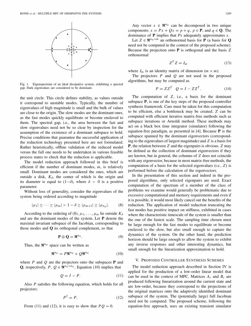
Dissipative systems exhibit a separation of timescales tofast and slow, resulting in the separation of eigenvaluesin the eigenspectrum of the linearized discrete-time system.Fig. 1 shows such a spectrum. The slow modes correspondto eigenvalues of high magnitude, i.e., close to, or outside of,


Fig. 1. Eigenspectrum of an ideal dissipative system, exhibiting a spectralgap. Dark eigenvalues are considered to be dominant.

the unit circle. This circle defines stability, as values outsideit correspond to unstable modes. Typically, the number ofeigenvalues of high magnitude is small and the bulk of valuesare close to the origin. The slow modes are the dominant ones,as the fast modes quickly equilibrate or become enslaved tothem. The spectral gap, i.e., the area between the fast andslow eigenvalues need not be so clear by inspection for theassumption of the existence of a dominant subspace to hold.Precise conditions that guarantee the successful application ofthe reduction technology presented here are not formulated.Rather heuristically, offline validation of the reduced modelversus the full one needs to be undertaken in various feasibleprocess states to check that the reduction is applicable.

The model reduction approach followed in this brief isefficient if the number of dominant modes, m, is relativelysmall. Dominant modes are considered the ones, which areoutside a disk, Kδ , the center of which is the origin andits diameter is equal to (1−δ), where δ > 0 is a positiveparameter.

Without loss of generality, consider the eigenvalues of thesystem being ordered according to magnitude

|μ1| ≥ · · · ≥ |μm | > 1 − δ ≥ |μm+1| ≥ |μnst |. (8)

According to the ordering of (8), μ1, . . . , μm lie outside Kδ

and are the dominant modes of the system. Let P denote themaximal invariant subspace of the Jacobian, corresponding tothose modes and Q its orthogonal complement, so that

P ⊕ Q = �nst . (9)

Thus, the �nst space can be written as

�nst = P�nst + Q�nst (10)

where P and Q are the projectors onto the subspaces P andQ, respectively, P , Q ∈ �nst×nst . Equation (10) implies that

Q = I − P. (11)

Also P satisfies the following equation, which holds for allprojectors:

P2 = P. (12)

From (11) and (12), it is easy to show that P Q = 0.

Any vector x ∈ �nst can be decomposed in two uniquecomponents: x = Px + Qx = p + q , p ∈ P, and q ∈ Q. Thedominance of P implies that Px adequately approximates x .

Let Z ∈ �nst×m an orthonormal basis for P (a basis for Qneed not be computed in the context of the proposed scheme).Because the projection onto P is orthogonal and the basis Zorthonormal

Z T Z = Im (13)

where Im is an identity matrix of dimension (m × m).The projectors P and Q are not used in the proposed

algorithms, but may be computed as

P = Z Z T Q = I − Z Z T . (14)

The computation of Z , i.e., a basis for the dominantsubspace P, is one of the key steps of the proposed controllersynthesis framework. Care must be taken for this computationto be efficient, else a bottleneck may be created. Z can becomputed with efficient iterative matrix-free methods such assubspace iterations or Arnoldi method. These methods mayact on a black box time integrator (simulator) following theequation-free paradigm, as presented in [4]. Because P is thesubspace spanned by the dominant eigenvectors (correspond-ing to the eigenvalues of largest magnitude) and Z is a basis forP, the relation between Z and the eigenpairs is obvious. Z maybe defined as the collection of dominant eigenvectors if theyare known, but in general, the columns of Z does not coincidewith any eigenvector, because in most matrix-free methods, thecomputation of a basis for the selected eigenvalues (i.e., Z) isperformed before the calculation of the eigenvectors.

In the presentation of this section and indeed in the pro-posed algorithms, only selected eigenpairs are used. Exactcomputation of the spectrum of a member of the class ofproblems we examine would generally be problematic due toexcessive computational and memory requirements and even ifit is possible, it would most likely cancel out the benefits of thereduction. The application of model reduction truncating thefast modes has positive impact on stiffness, exhibited in caseswhere the characteristic timescale of the system is smaller thanthe one of the fastest scale. The sampling time chosen mustbe large enough for the fast modes to equilibrate or becomeenslaved to the slow, but also small enough to capture thedynamics of the system. On the other hand, the predictionhorizon should be large enough to allow the system to exhibitany inverse responses and other interesting dynamics, butsmall enough for the linearization approximation to hold.

V. PROPOSED CONTROLLER SYNTHESIS SCHEMES

The model reduction approach described in Section IV isapplied for the production of a low-order linear model thatcan be used in the context of MPC. Matrices Ac and Bc areproduced following linearization around the current state andare low-order, because they correspond to the projections ofthe original matrices onto the adaptively identified dominantsubspace of the system. The (potentially large) full Jacobianneed not be computed. The proposed scheme, following theequation-free approach, uses an existing transient simulator


to approximate the products of approximate Jacobian Fx withgiven vectors. Matrix-free methodologies are employed, actingdirectly on the simulator, appropriately initialized and used fora certain reporting horizon as described in detail in [4].

The maximal invariant subspace belonging to the m eigen-values of Fx of largest magnitude is considered as the dom-inant subspace. This eigenspace can be identified using amatrix-free method. Here, an implementation of the implicitlyrestarted Arnoldi method is used. This procedure results in anorthonormal basis Z ∈ �nst×m of the dominant subspace.

The basis Z is used to project the state vector x onto thedominant subspace to obtain a reduced state vector ξ ∈ �m

ξ = Z T x . (15)

Using this reduced state, we can get a reduced order system

ξ (t) = Ac,redξ(t) + Bc,redu(t)

y(t) = C Zξ(t) + Du(t). (16)

The reduced Jacobian, H ∈ �m×m is defined as

H = Z T Fx Z (17)

and can be computed efficiently following a two-step proce-dure described in [4]. It can be shown that

Ac,red = I − H. (18)

Matrix Bc,red is computed with numerical perturbationson the simulator similarly to H and comprises a projectiononto P.

The linearization scheme is adaptive, hence matrices Ac,redand Bc,red are evaluated at the linearization points. The sys-tem (16) needs to be transformed to discrete-time, to obtain

ξ(k + 1) = Aξ(k) + Bu(k)

y(k) = C Zξ(k) + Du(k). (19)

The low-order linear model of (19) can be used to formulatean MPC optimization problem as in [4]

U = arg minU

Np∑k=1

∥∥(y(t + kTs |t) − r(t + kTs)

)∥∥2Qw

+Nc∑

k=1

‖(u(t + kTs |t) − u(t + (k − 1)Ts |t))‖2Rw

s.t. ξ (t + (k + 1)Ts |t) = Aξ (t + kTs |t) + Bu(t + kTs |t)y(t + kTs |t) = C Z T ξ (t + kTs |t) + Du(t + kTs |t)ulower ≤ u ≤ uupper k = 1, 2, . . . Np . (20)

The quasi-peak (QP) in (20) is reduced and will be feasibleif the problem is feasible as a consequence of [23, Th. 1]. Theoptimization problem formulation is conventional (see [24])and includes terms penalizing the deviation from the set pointand the required control energy, i.e., the difference betweentwo consecutive control decisions. The MPC controller weemploy does not include a terminal constraint for stability. In[15], stability without terminal constraints is discussed. Thisbrief focuses on efficient model approximation and is com-patible with MPC algorithms guaranteeing stability. Caution,

however, is advised, because some of the desired properties ofthe underlying linear controller may be compromised, becauseof traversing between regions of different surrogate models andbecause of truncating the fast modes for model reduction.

Following the MMPC notion, the controller is reformulatedwhenever the model needs to be updated. Here we considertwo approaches in updating the underlying linear reducedmodel and hence controller—an off-line and an online one.

The projection onto the dominant subspace has minimalimpact on stability, because this subspace includes all poten-tially unstable modes. Furthermore, it is easy to prove usingthe theorem in [23] that the extrema of the full optimizationproblem are extrema of the reduced one also, which eliminatesanother potential source of instability. This is not to saythat there is no chance of obtaining a destabilizing controllerusing the proposed methods. This behavior is observed ifthe full optimization problem has no feasible solution, or incases where the number of modes is underestimated, leadingto significant mismatch to the full model, hence erroneousidentification of P. Also, in some problems, convergence toan optimal solution not satisfying the full problem may beobtained (see [23]).

A. Off-LineProcedure

A nontrivial part of the overall procedure is performed off-line to reduce the online cost of the algorithm. The outcomeof this procedure is a model pool, i.e., a database, each recordof which contains [ j, t j

L, t jR, A j , B j , Z j ]. Records correspond

to nonoverlapping regions and provide data that the onlinecontroller can use. To set up this model pool, a list ofrealistic scenarios (process conditions) is determined and off-line transient simulations are run. For each of them:

1) the optimal number of linearization points n for staticTPWL is determined and the linearization states areidentified;

2) adaptive TPWL is applied to minimize n;3) for each of the linearization states, a base Z of the

dominant subspace P is computed;4) for each of the intervals computed with adaptive TPWL,

a record is added in the model pool containing processconditions, time interval of the model, as well as A, B ,and Z .

B. Online Procedure I: Off-Line Gain Scheduling Approach

According to this paradigm, the model is updated accordingto process time. The plant trajectory is computed a priori,solving either a simulation or an optimal control problem andthe time linearization intervals, according to the procedureof Section III, are computed from this trajectory. A poolof temporal regions are obtained, in which the process isapproximated with a linear model, along with the reducedmatrices of (19). Real process time is used to match thenonlinear model with a linear model stored at the model bank(for the same process conditions). This linear model is usedin an MPC algorithm. For the first interval ( j = 1), t j

L = 0.At time t , we use the matrices A j , B j , and Z j , corresponding


to the interval j , for which t jL ≤ t < t j

R . The model is updatedwhen the process time exceeds t j

R .This approach has the advantage that the model map is

known off-line. This means that state observation requirementsonline are minimal and that the control law may be computedexplicitly off-line following the multiparametric MPC strategy[19]. The disadvantage is that disturbances are difficult tomodel and that uncertainties in the operating parameters areunaccounted for. If the model is sufficiently linear in the regionin question, these limitations pose no problem. This sort ofgain scheduling is used in [5] and [6].

C. Online Procedure II: Online (Linear) Model Identification

Online gain scheduling tries to address some of the short-comings of the off-line strategy. It is more flexible andaccounts for the unmeasured disturbances effecting on thetemporal evolution of the states. Furthermore, the linearizationneed not be performed along one trajectory only. Obviously,the more the reference trajectories are used, the higher arethe number of resulting linear models. An excessive numberbalances the complexity of the original nonlinear model withthe computational effort of traversing the model pool toidentify the local reduced model.

A record j of the model database contains[ j, ξ j , A j , B j , Z j ]. In comparison to the model bankof Section V-B, the linearization times are not used, but thelinearization point (state) is included. Update of the model isperformed at each of the sampling times or less frequently.The model at time instance i is expressed as a weightedlinear combination of the models in the model pool. Thecomputation of the weighted model followed the rationale of[17]. At each sampling instance:

1) the system state x is observed;2) the distance between the state and the linearization

points is computed, d j = ‖x − Z jξ j ‖2, j = 1, . . . , n;3) a weight for each of the models in the model pool is

computed, w j = exp(−βd j

ζ ), with ζ = min j=1,...,nd j ,β > 0;

4) the sum of weights is calculated, � = ∑nj=1 w j ;

5) the weights are normalized, w j = w j /�.With w j at hand, the model matrices are computed as

Ai =n∑

j=1

w j A j Bi =n∑

j=1

w j B j . (21)

The basis Z used is the one corresponding to the closestlinearization point to the current state. Update of the matricesleads to the reformulation of QP (20), increasing the onlinecomputational cost. This increase is insignificant for worksta-tions, but may be of importance to process hardware.

VI. CASE STUDY: STABILIZATION OF A

TUBULAR REACTOR

The behavior and efficiency of the proposed algorithmsis illustrated by applying them for the control of a tubularreactor with recycle, where a first-order, elementary irre-versible, exothermic reaction takes place, A → B . There are

Fig. 2. Sketch of a tubular reactor with recycle stream.

two state variables: the dimensionless concentration x1 andthe dimensionless temperature x2. The model for the reactorconsists of two parabolic PDEs [25]

∂x1

∂ t= 1

Pe1

∂2x1

∂y2 − ∂x1

∂y− Da · x1 exp

(γ x2

1 + x2

)∂x2

∂ t= 1

Pe2

∂2x2

∂y2 − ∂x2

∂y+ C Da · x1 exp

(γ x2

1 + x2

)+β(x2w − x2) (22)

where y is the dimensionless longitudinal coordinate, r is therecycle ratio, Da is the Damköhler number, Pe1 is the Peckletnumber for mass transport, and Pe2 for heat transport, β adimensionless heat transfer coefficient, C is the dimensionlessadiabatic temperature rise, x2w the dimensionless adiabaticwall temperature, and γ the dimensionless activation energy.The boundary conditions for this model are

∂x1

∂y= −Pe1

[(1 − r)x0

1 + r x1|y=1 − r x1|y=0

]∂x2

∂y= −Pe2

[(1−r)x0

2 + r x2|y=1 − r x2|y=0

]at y = 0 (23)

∂x1

∂y= 0,

∂x2

∂y= 0 at y = 1. (24)

The initial conditions of the system are x01 = 0, x0

2 = 0.The values of the parameters chosen are Da = 0.1, Pe1 =Pe2 = 7.0, γ = 10.0, β = 2.0, and C = 2.5. Forthe identification of bases for the dominant subspaces ofthe system, Arnoldi method is used and warm-started. Thetolerance by which Z is computed is 10−6, although muchhigher tolerances are tested successfully. The sampling timeis 0.01.

The jacket of the reactor is considered to be comprisedof eight heat exchangers of equal surface, the temperaturesof which can be controlled independently and comprise themanipulated variables for the control problem. Hence thedimensionless wall temperature x2w is considered to varyspatially, as a function of the control actions

x2w(y) =8∑

j=1

(H (y − y j−1) − H (y) − yi

)u j (t). (25)

With yi = i/8, i = 0, 1, . . . , 8, x2w j (t), j = 1, 2, . . . , 8, isthe dimensionless temperature of the cooling zone for time tand H (·) is the Heaviside step function.

The exit temperature of the reactor is the output of thesystem. A schematic of the reactor is given in Fig. 2.

The model equations are semidiscretized in space with thefinite element method and time marching follows an implicitEuler integration scheme. The discretization is on a mesh of16 nodes, resulting in 32 ordinary differential equations. Thesimulator for the reactor is used by the controller as black box


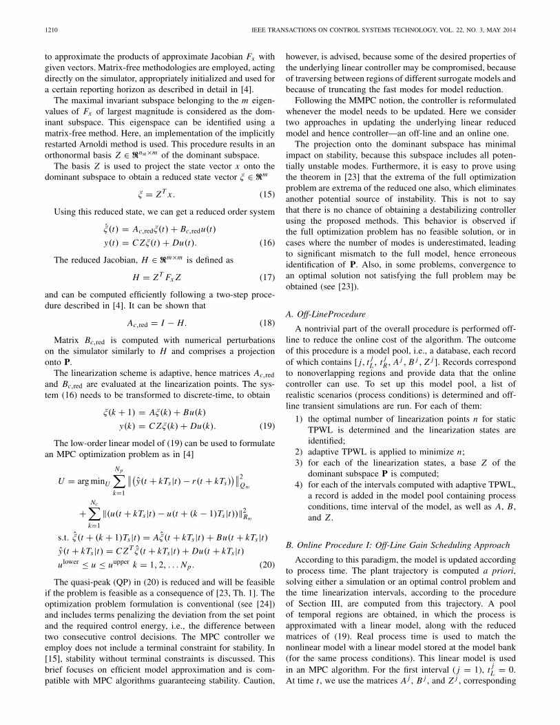
Fig. 3. Dynamic profile of output variable for r = 0 (dashed line) andr = 0.5 (solid line).

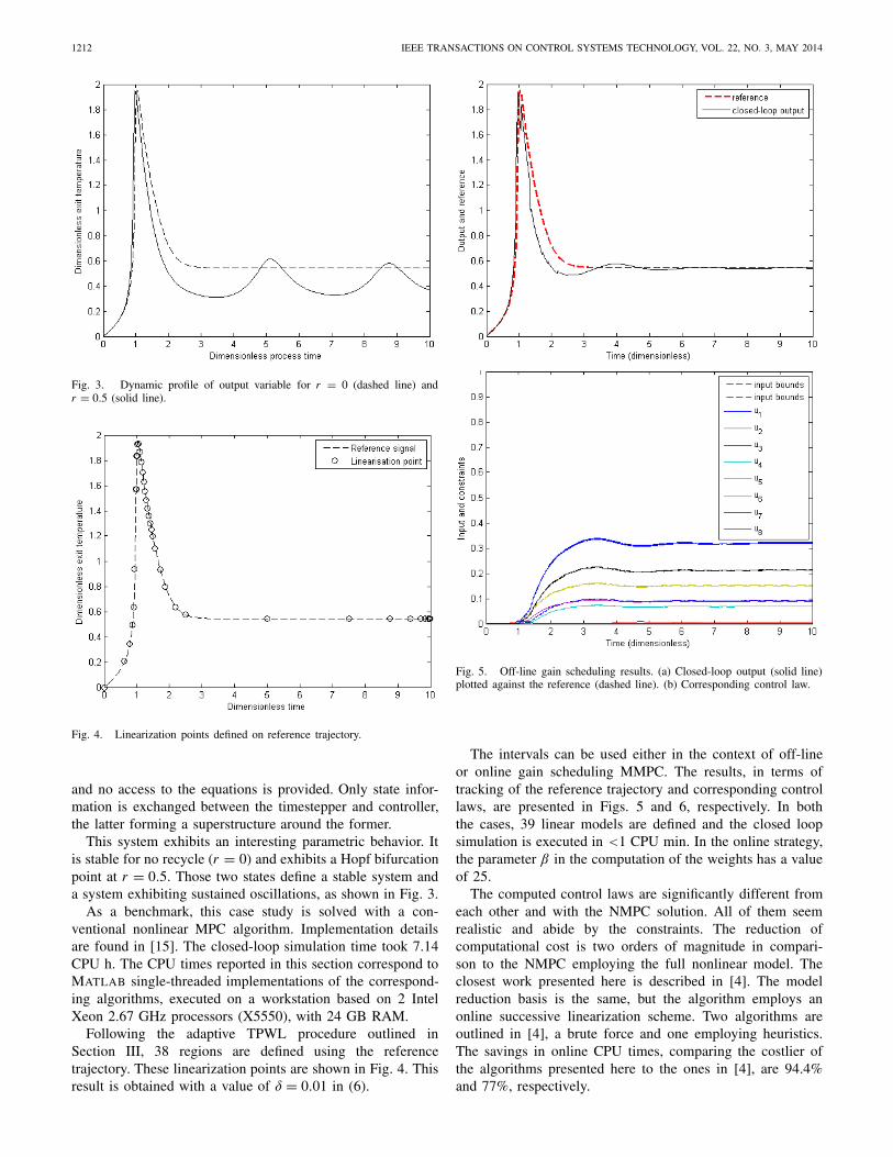
Fig. 4. Linearization points defined on reference trajectory.

and no access to the equations is provided. Only state infor-mation is exchanged between the timestepper and controller,the latter forming a superstructure around the former.

This system exhibits an interesting parametric behavior. Itis stable for no recycle (r = 0) and exhibits a Hopf bifurcationpoint at r = 0.5. Those two states define a stable system anda system exhibiting sustained oscillations, as shown in Fig. 3.

As a benchmark, this case study is solved with a con-ventional nonlinear MPC algorithm. Implementation detailsare found in [15]. The closed-loop simulation time took 7.14CPU h. The CPU times reported in this section correspond toMATLAB single-threaded implementations of the correspond-ing algorithms, executed on a workstation based on 2 IntelXeon 2.67 GHz processors (X5550), with 24 GB RAM.

Following the adaptive TPWL procedure outlined inSection III, 38 regions are defined using the referencetrajectory. These linearization points are shown in Fig. 4. Thisresult is obtained with a value of δ = 0.01 in (6).

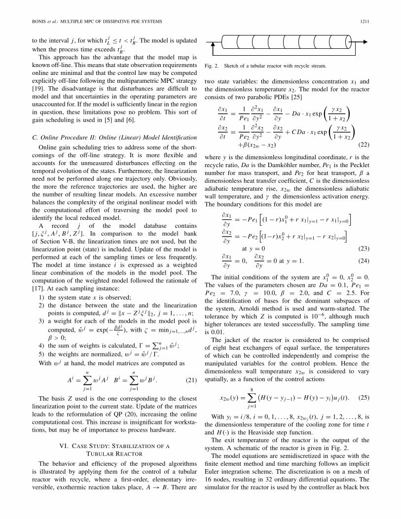
Fig. 5. Off-line gain scheduling results. (a) Closed-loop output (solid line)plotted against the reference (dashed line). (b) Corresponding control law.

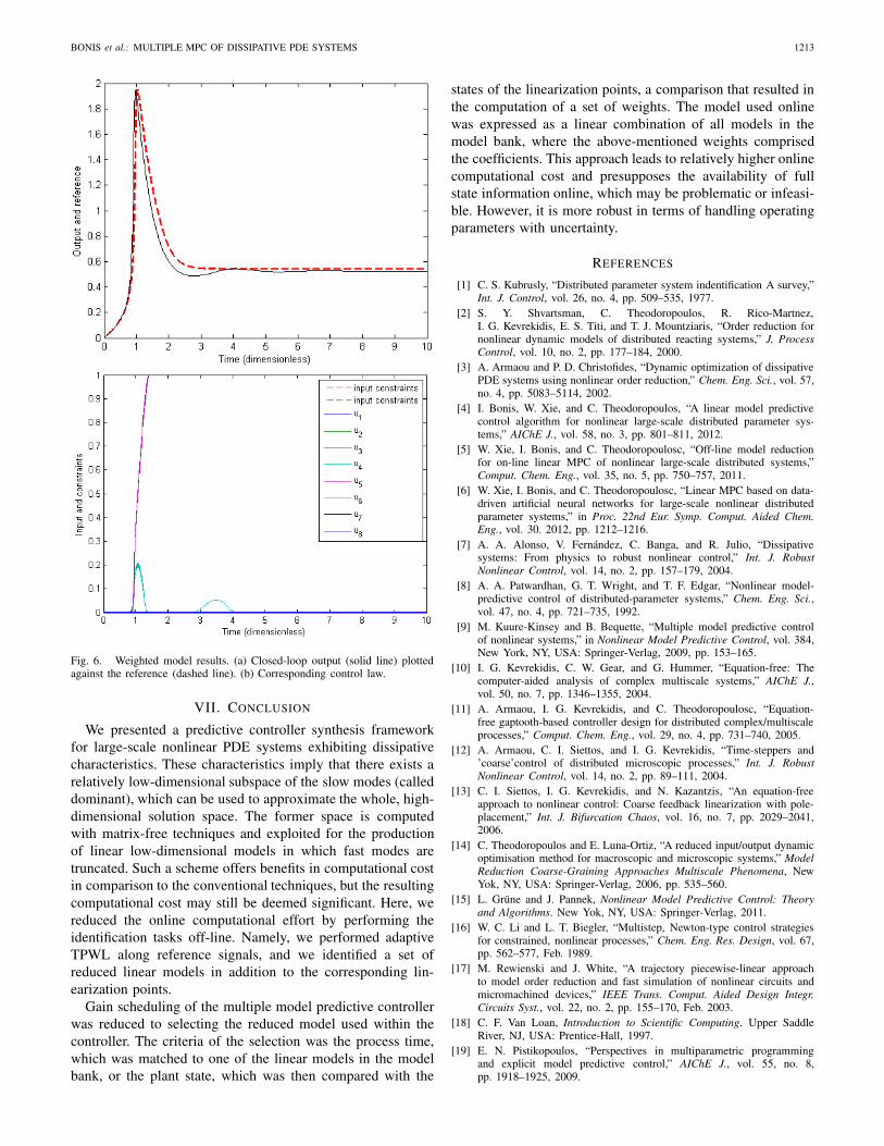
The intervals can be used either in the context of off-lineor online gain scheduling MMPC. The results, in terms oftracking of the reference trajectory and corresponding controllaws, are presented in Figs. 5 and 6, respectively. In boththe cases, 39 linear models are defined and the closed loopsimulation is executed in <1 CPU min. In the online strategy,the parameter β in the computation of the weights has a valueof 25.

The computed control laws are significantly different fromeach other and with the NMPC solution. All of them seemrealistic and abide by the constraints. The reduction ofcomputational cost is two orders of magnitude in compari-son to the NMPC employing the full nonlinear model. Theclosest work presented here is described in [4]. The modelreduction basis is the same, but the algorithm employs anonline successive linearization scheme. Two algorithms areoutlined in [4], a brute force and one employing heuristics.The savings in online CPU times, comparing the costlier ofthe algorithms presented here to the ones in [4], are 94.4%and 77%, respectively.


Fig. 6. Weighted model results. (a) Closed-loop output (solid line) plottedagainst the reference (dashed line). (b) Corresponding control law.

VII. CONCLUSION

We presented a predictive controller synthesis frameworkfor large-scale nonlinear PDE systems exhibiting dissipativecharacteristics. These characteristics imply that there exists arelatively low-dimensional subspace of the slow modes (calleddominant), which can be used to approximate the whole, high-dimensional solution space. The former space is computedwith matrix-free techniques and exploited for the productionof linear low-dimensional models in which fast modes aretruncated. Such a scheme offers benefits in computational costin comparison to the conventional techniques, but the resultingcomputational cost may still be deemed significant. Here, wereduced the online computational effort by performing theidentification tasks off-line. Namely, we performed adaptiveTPWL along reference signals, and we identified a set ofreduced linear models in addition to the corresponding lin-earization points.

Gain scheduling of the multiple model predictive controllerwas reduced to selecting the reduced model used within thecontroller. The criteria of the selection was the process time,which was matched to one of the linear models in the modelbank, or the plant state, which was then compared with the

states of the linearization points, a comparison that resulted inthe computation of a set of weights. The model used onlinewas expressed as a linear combination of all models in themodel bank, where the above-mentioned weights comprisedthe coefficients. This approach leads to relatively higher onlinecomputational cost and presupposes the availability of fullstate information online, which may be problematic or infeasi-ble. However, it is more robust in terms of handling operatingparameters with uncertainty.

REFERENCES

[1] C. S. Kubrusly, “Distributed parameter system indentification A survey,”Int. J. Control, vol. 26, no. 4, pp. 509–535, 1977.

[2] S. Y. Shvartsman, C. Theodoropoulos, R. Rico-Martnez,I. G. Kevrekidis, E. S. Titi, and T. J. Mountziaris, “Order reduction fornonlinear dynamic models of distributed reacting systems,” J. ProcessControl, vol. 10, no. 2, pp. 177–184, 2000.

[3] A. Armaou and P. D. Christofides, “Dynamic optimization of dissipativePDE systems using nonlinear order reduction,” Chem. Eng. Sci., vol. 57,no. 4, pp. 5083–5114, 2002.

[4] I. Bonis, W. Xie, and C. Theodoropoulos, “A linear model predictivecontrol algorithm for nonlinear large-scale distributed parameter sys-tems,” AIChE J., vol. 58, no. 3, pp. 801–811, 2012.

[5] W. Xie, I. Bonis, and C. Theodoropoulosc, “Off-line model reductionfor on-line linear MPC of nonlinear large-scale distributed systems,”Comput. Chem. Eng., vol. 35, no. 5, pp. 750–757, 2011.

[6] W. Xie, I. Bonis, and C. Theodoropoulosc, “Linear MPC based on data-driven artificial neural networks for large-scale nonlinear distributedparameter systems,” in Proc. 22nd Eur. Symp. Comput. Aided Chem.Eng., vol. 30. 2012, pp. 1212–1216.

[7] A. A. Alonso, V. Fernández, C. Banga, and R. Julio, “Dissipativesystems: From physics to robust nonlinear control,” Int. J. RobustNonlinear Control, vol. 14, no. 2, pp. 157–179, 2004.

[8] A. A. Patwardhan, G. T. Wright, and T. F. Edgar, “Nonlinear model-predictive control of distributed-parameter systems,” Chem. Eng. Sci.,vol. 47, no. 4, pp. 721–735, 1992.

[9] M. Kuure-Kinsey and B. Bequette, “Multiple model predictive controlof nonlinear systems,” in Nonlinear Model Predictive Control, vol. 384,New York, NY, USA: Springer-Verlag, 2009, pp. 153–165.

[10] I. G. Kevrekidis, C. W. Gear, and G. Hummer, “Equation-free: Thecomputer-aided analysis of complex multiscale systems,” AIChE J.,vol. 50, no. 7, pp. 1346–1355, 2004.

[11] A. Armaou, I. G. Kevrekidis, and C. Theodoropoulosc, “Equation-free gaptooth-based controller design for distributed complex/multiscaleprocesses,” Comput. Chem. Eng., vol. 29, no. 4, pp. 731–740, 2005.

[12] A. Armaou, C. I. Siettos, and I. G. Kevrekidis, “Time-steppers and’coarse’control of distributed microscopic processes,” Int. J. RobustNonlinear Control, vol. 14, no. 2, pp. 89–111, 2004.

[13] C. I. Siettos, I. G. Kevrekidis, and N. Kazantzis, “An equation-freeapproach to nonlinear control: Coarse feedback linearization with pole-placement,” Int. J. Bifurcation Chaos, vol. 16, no. 7, pp. 2029–2041,2006.

[14] C. Theodoropoulos and E. Luna-Ortiz, “A reduced input/output dynamicoptimisation method for macroscopic and microscopic systems,” ModelReduction Coarse-Graining Approaches Multiscale Phenomena, NewYok, NY, USA: Springer-Verlag, 2006, pp. 535–560.

[15] L. Grüne and J. Pannek, Nonlinear Model Predictive Control: Theoryand Algorithms. New Yok, NY, USA: Springer-Verlag, 2011.

[16] W. C. Li and L. T. Biegler, “Multistep, Newton-type control strategiesfor constrained, nonlinear processes,” Chem. Eng. Res. Design, vol. 67,pp. 562–577, Feb. 1989.

[17] M. Rewienski and J. White, “A trajectory piecewise-linear approachto model order reduction and fast simulation of nonlinear circuits andmicromachined devices,” IEEE Trans. Comput. Aided Design Integr.Circuits Syst., vol. 22, no. 2, pp. 155–170, Feb. 2003.

[18] C. F. Van Loan, Introduction to Scientific Computing. Upper SaddleRiver, NJ, USA: Prentice-Hall, 1997.

[19] E. N. Pistikopoulos, “Perspectives in multiparametric programmingand explicit model predictive control,” AIChE J., vol. 55, no. 8,pp. 1918–1925, 2009.


[20] S. Dubljevic, P. Mhaskar, N. H. E. Farra, and P. D. Christofides,“Predictive control of transport-reaction processes,” Comput. Chem.Eng., vol. 29, pp. 2335–2345, Oct. 2005.

[21] S. Dubljevic, N. H. El-Farra, P. Mhaskar, and P. D. Christofides,“Predictive control of parabolic PDEs with state and control constraints,”Int. J. Robust Nonlinear Control, vol. 16, no. 16, pp. 749–772, 2006.

[22] G. M. Shroff and H. B. Keller, “Stabilization of unstable procedures:The recursive projection method,” SIAM J. Numerical Anal., vol. 30,no. 4, pp. 1099–1120, 1993.

[23] I. Bonis and C. Theodoropoulos, “Model reduction-based optimizationusing large-scale steady-state simulators,” Chem. Eng. Sci., vol. 69,pp. 69–80, Feb. 2012.

[24] A. G. Wills and W. P. Heath, “Application of barrier function basedmodel predictive control to an edible oil refining process,” J. ProcessControl, vol. 15, no. 2, pp. 183–200, 2005.

[25] K. F. Jensen and W. H. Ray, “The bifurcation behavior of tubu-lar reactors,” Chem. Eng. Sci., vol. 37, no. 2, pp. 199–222,1982.

Documents

Multiple Model Predictive Control of Dissipative PDE Systems