multiple linear regression - floppybunny.org · Practical Companion to Statistics at Square 2 Multiple Linear Regression Robin Beaumont [email protected] D:\web_sites_mine\HIcourseweb

$Page 1: multiple linear regression - floppybunny.org · Practical Companion to Statistics at Square 2 Multiple Linear Regression Robin Beaumont robin@organplayers.co.uk D:\web_sites_mine\HIcourseweb$
Practical Companion to Statistics at Square 2 Multiple Linear Regression

Robin Beaumont [email protected] D:\web_sites_mine\HIcourseweb new\stats\statistics2\mult_lin_reg_campbell_companian.docx page 1 of 30

Practical Companion to Statistics at

Square 2 by Micheal Campbell

Multiple Linear Regression

Written by: Robin Beaumont e-mail: [email protected]

Date last updated Monday, 29 November 2010

Version: 1

Important before you start:

Get a copy of Statistics at square 2 by Micheal Campbell

Have worked through Simple regression chapter at:

http://www.robin-beaumont.co.uk/virtualclassroom/stats/course1.html




How this document should be used: This document has been designed to be suitable for both web based and face-to-face teaching. The text has been made to be as interactive as possible with exercises, Multiple Choice Questions (MCQs) and web based exercises.

If you are using this document as part of a web-based course you are urged to use the online discussion board to discuss the issues raised in this document and share your solutions with other students.

This document is part of a series see: http://www.robin-beaumont.co.uk/virtualclassroom/stats/course1.html

And


Who this document is aimed at: This document is aimed at those people who want to learn more about statistics in a practical way. It is the eighth in the series.

I hope you enjoy working through this document. Robin Beaumont

Acknowledgments

My sincere thanks go to Claire Nickerson for not only proofreading several drafts but also providing additional material and technical advice.





Contents 1. INTRODUCTION .................................................................................................................................................... 4

2. PARTIAL AND PART CORRELATION........................................................................................................................ 4

3. GRAPHICAL INTERPRETATIONS ............................................................................................................................. 6

4. MULTIPLE LINEAR REGRESSION............................................................................................................................. 8

4.1 TWO CONTINUOUS VARIABLES ............................................................................................................................... 9 4.1.1 The Collinearity problem ........................................................................................................................... 9 4.1.2 Venn diagrams and Correlation equations ................................................................................................11

5. ONE CONTINUOUS ONE DICHOTOMOUS .............................................................................................................13

6. TWO INDEPENDENT VARIABLES ONE CONTINUOUS ONE DICHOTOMOUS WITH INTERACTION ...........................19

7. TWO NOMINAL INDEPENDENT VARIABLES ..........................................................................................................23

7.1 ANALYSING NOMINAL VARIABLES THE ANOVA APPROACH ..........................................................................................27

8. ASSUMPTIONS, RESIDUALS, LEVERAGE AND INFLUENCE .....................................................................................28

9. STEPWISE REGRESSION ETC. ................................................................................................................................28

10. REPORTING AND READING THE RESULTS OF MULTIPLE LINEAR REGRESSION ..................................................28

11. EXERCISES ........................................................................................................................................................28

12. SUMMARY .......................................................................................................................................................29

13. REFERENCES.....................................................................................................................................................30

14. APPENDIX - SOME GRAPHICAL OPTIONS IN R ..................................................................................................30



1. Introduction

This handout provides both additional theoretical material and a practical accompaniment to the Multiple Linear Regression chapter from Micheal Campbell's excellent book, Statistics at square two (bmj books). The book is remarkable, and the multiple regression chapter in particular, for covering a large amount of ground in very few pages, however one of the limitations is that it is rather didactic and does not provide guided practical exercises or discussion of some of the maths behind the process.

Regression analysis focuses on three inter-related aspects:

Overall fit - R squared (R2) assessment

Parameter estimation / evaluation B's and betas (β) etc

Assessment of statistical validity of model – LINE criteria extrapolation, subgroups, causal implications etc. (see my simple linear regression chapter)

We have discussed many of the above aspects in the chapter on simple linear regression, however the first two issues become more complex with the situation of more than one independent (i.e. input) variable. To interpret the results a particular way it is necessary to understand two more complex types of correlation, called partial and part (also called semipartial) correlation.

2. Partial and Part correlation

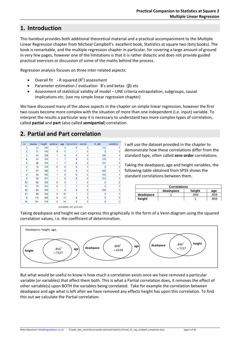
I will use the dataset provided in the chapter to demonstrate how these correlations differ from the standard type, often called zero order correlations.

Taking the deadspace, age and height variables, the following table obtained from SPSS shows the standard correlations between them.

Taking deadspace and height we can express this graphically in the form of a Venn diagram using the squared correlation values, i.e. the coefficient of determination.

But what would be useful to know is how much a correlation exists once we have removed a particular variable (or variables) that affect them both. This is what a Partial correlation does, it removes the effect of other variable(s) upon BOTH the variables being correlated. Take for example the correlation between deadspace and age what is left after we have removed any effects height has upon this correlation. To find this out we calculate the Partial correlation.

Correlations

deadspace height age

deadspace 1 .846 .808

height 1 .856

age deadspace

.8082

=.6528

Deadspace, height, age,

height deadspace .846

2

=.7157 age height

.8562

=.7327

[campbell_mlr_p12.sav]



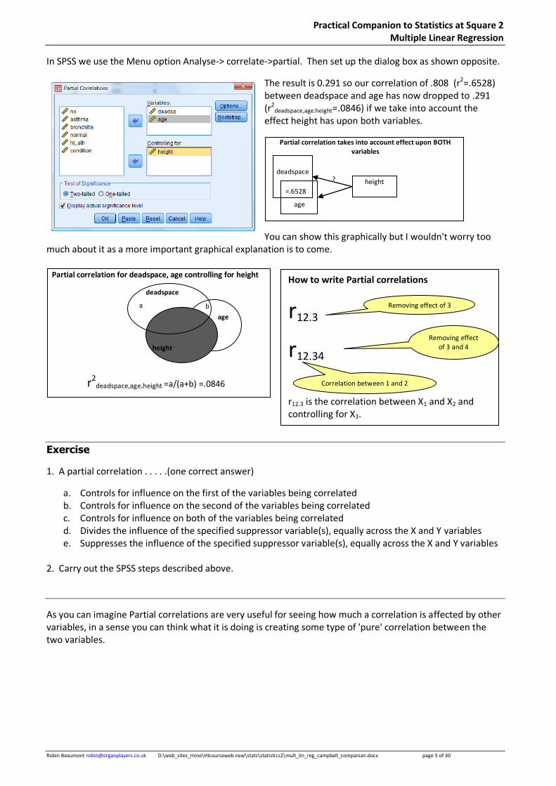
In SPSS we use the Menu option Analyse-> correlate->partial. Then set up the dialog box as shown opposite.

The result is 0.291 so our correlation of .808 (r2=.6528) between deadspace and age has now dropped to .291 (r2

deadspace,age.height=.0846) if we take into account the effect height has upon both variables.

You can show this graphically but I wouldn't worry too much about it as a more important graphical explanation is to come.

Exercise

1. A partial correlation . . . . .(one correct answer)

a. Controls for influence on the first of the variables being correlated b. Controls for influence on the second of the variables being correlated c. Controls for influence on both of the variables being correlated d. Divides the influence of the specified suppressor variable(s), equally across the X and Y variables e. Suppresses the influence of the specified suppressor variable(s), equally across the X and Y variables

2. Carry out the SPSS steps described above.

As you can imagine Partial correlations are very useful for seeing how much a correlation is affected by other variables, in a sense you can think what it is doing is creating some type of 'pure' correlation between the two variables.

deadspace

age

height

Partial correlation takes into account effect upon BOTH variables

=.6528

?

age

deadspace

a

Partial correlation for deadspace, age controlling for height


height

b

r2deadspace,age.height =a/(a+b) =.0846

How to write Partial correlations

r12.3

r12.34

r12.3 is the correlation between X1 and X2 and controlling for X3.

Correlation between 1 and 2

Removing effect of 3 and 4

Removing effect of 3



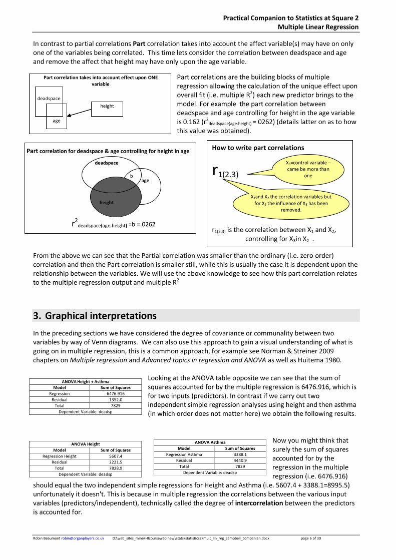
How to write part correlations

r1(2.3)

r1(2.3) is the correlation between X1 and X2, controlling for X3in X2 .

age

deadspace

Part correlation for deadspace & age controlling for height in age


height

b

r2deadspace(age.height) =b =.0262

In contrast to partial correlations Part correlation takes into account the affect variable(s) may have on only one of the variables being correlated. This time lets consider the correlation between deadspace and age and remove the affect that height may have only upon the age variable.

Part correlations are the building blocks of multiple regression allowing the calculation of the unique effect upon overall fit (i.e. multiple R2) each new predictor brings to the model. For example the part correlation between deadspace and age controlling for height in the age variable is 0.162 (r2

deadspace(age.height) = 0262) (details latter on as to how this value was obtained).

From the above we can see that the Partial correlation was smaller than the ordinary (i.e. zero order) correlation and then the Part correlation is smaller still, while this is usually the case it is dependent upon the relationship between the variables. We will use the above knowledge to see how this part correlation relates to the multiple regression output and multiple R2

3. Graphical interpretations

In the preceding sections we have considered the degree of covariance or communality between two variables by way of Venn diagrams. We can also use this approach to gain a visual understanding of what is going on in multiple regression, this is a common approach, for example see Norman & Streiner 2009 chapters on Multiple regression and Advanced topics in regression and ANOVA as well as Huitema 1980.

Looking at the ANOVA table opposite we can see that the sum of squares accounted for by the multiple regression is 6476.916, which is for two inputs (predictors). In contrast if we carry out two independent simple regression analyses using height and then asthma (in which order does not matter here) we obtain the following results.

Now you might think that surely the sum of squares accounted for by the regression in the multiple regression (i.e. 6476.916)

should equal the two independent simple regressions for Height and Asthma (i.e. 5607.4 + 3388.1=8995.5) unfortunately it doesn't. This is because in multiple regression the correlations between the various input variables (predictors/independent), technically called the degree of intercorrelation between the predictors is accounted for.

ANOVA Height + Asthma

Model Sum of Squares

Regression 6476.916

Residual 1352.0

Total 7829

Dependent Variable: deadsp

ANOVA Height


Regression Height 5607.4

Residual 2221.5

Total 7828.9


ANOVA Asthma


Regression Asthma 3388.1

Residual 4440.9

Total 7829


Correlation between 1 and 2

deadspace

age

height

Part correlation takes into account effect upon ONE variable

X1 X2 where effect of X3 has been removed from it

X3=control variable – came be more than

one

X1

X1and X2 the correlation variables but for X2 the influence of X3 has been

removed.



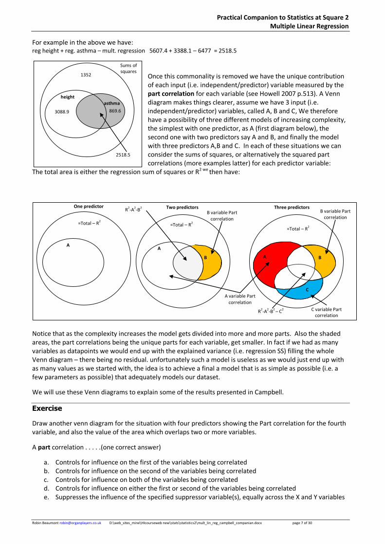
For example in the above we have: reg height + reg. asthma – mult. regression 5607.4 + 3388.1 – 6477 = 2518.5

Once this commonality is removed we have the unique contribution of each input (i.e. independent/predictor) variable measured by the part correlation for each variable (see Howell 2007 p.513). A Venn diagram makes things clearer, assume we have 3 input (i.e. independent/predictor) variables, called A, B and C, We therefore have a possibility of three different models of increasing complexity, the simplest with one predictor, as A (first diagram below), the second one with two predictors say A and B, and finally the model with three predictors A,B and C. In each of these situations we can consider the sums of squares, or alternatively the squared part correlations (more examples latter) for each predictor variable:

The total area is either the regression sum of squares or R2 we then have:

Notice that as the complexity increases the model gets divided into more and more parts. Also the shaded areas, the part correlations being the unique parts for each variable, get smaller. In fact if we had as many variables as datapoints we would end up with the explained variance (i.e. regression SS) filling the whole Venn diagram – there being no residual. unfortunately such a model is useless as we would just end up with as many values as we started with, the idea is to achieve a final a model that is as simple as possible (i.e. a few parameters as possible) that adequately models our dataset.

We will use these Venn diagrams to explain some of the results presented in Campbell.

Exercise

Draw another venn diagram for the situation with four predictors showing the Part correlation for the fourth variable, and also the value of the area which overlaps two or more variables.

A part correlation . . . . .(one correct answer)

a. Controls for influence on the first of the variables being correlated b. Controls for influence on the second of the variables being correlated c. Controls for influence on both of the variables being correlated d. Controls for influence on either the first or second of the variables being correlated e. Suppresses the influence of the specified suppressor variable(s), equally across the X and Y variables

=Total – R2

One predictor

A A

R2-A

2-B

2 Two predictors

=Total – R2

B variable Part correlation

B

A variable Part correlation

B

B variable Part correlation

A

R2-A

2-B

2 – C

2

=Total – R2

Three predictors

C variable Part correlation

C

1352

3088.9 869.6

asthma height

2518.5

Sums of squares



4. Multiple linear regression

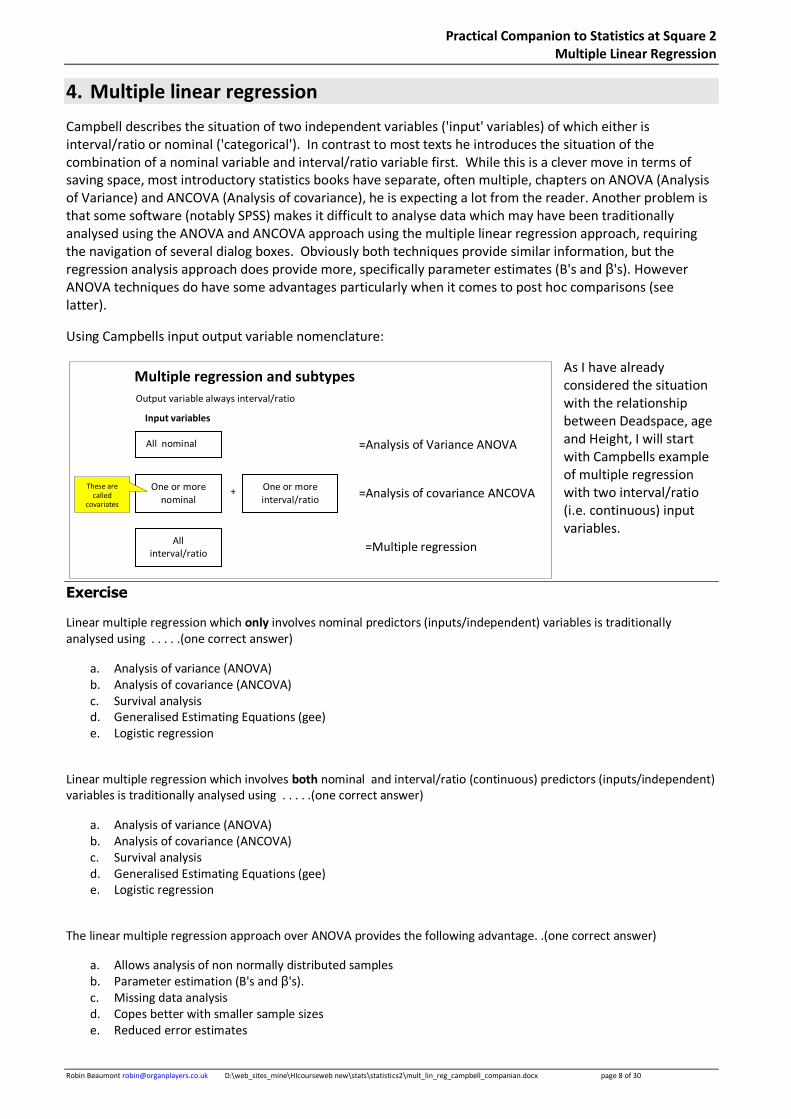
Campbell describes the situation of two independent variables ('input' variables) of which either is interval/ratio or nominal ('categorical'). In contrast to most texts he introduces the situation of the combination of a nominal variable and interval/ratio variable first. While this is a clever move in terms of saving space, most introductory statistics books have separate, often multiple, chapters on ANOVA (Analysis of Variance) and ANCOVA (Analysis of covariance), he is expecting a lot from the reader. Another problem is that some software (notably SPSS) makes it difficult to analyse data which may have been traditionally analysed using the ANOVA and ANCOVA approach using the multiple linear regression approach, requiring the navigation of several dialog boxes. Obviously both techniques provide similar information, but the regression analysis approach does provide more, specifically parameter estimates (B's and β's). However ANOVA techniques do have some advantages particularly when it comes to post hoc comparisons (see latter).

Using Campbells input output variable nomenclature:

As I have already considered the situation with the relationship between Deadspace, age and Height, I will start with Campbells example of multiple regression with two interval/ratio (i.e. continuous) input variables.

Exercise

Linear multiple regression which only involves nominal predictors (inputs/independent) variables is traditionally analysed using . . . . .(one correct answer)

a. Analysis of variance (ANOVA) b. Analysis of covariance (ANCOVA) c. Survival analysis d. Generalised Estimating Equations (gee) e. Logistic regression

Linear multiple regression which involves both nominal and interval/ratio (continuous) predictors (inputs/independent) variables is traditionally analysed using . . . . .(one correct answer)

a. Analysis of variance (ANOVA) b. Analysis of covariance (ANCOVA) c. Survival analysis d. Generalised Estimating Equations (gee) e. Logistic regression

The linear multiple regression approach over ANOVA provides the following advantage. .(one correct answer)

a. Allows analysis of non normally distributed samples b. Parameter estimation (B's and β's). c. Missing data analysis d. Copes better with smaller sample sizes e. Reduced error estimates

Output variable always interval/ratio

Input variables

All nominal

One or more nominal

+ One or more interval/ratio

All interval/ratio

=Multiple regression

=Analysis of Variance ANOVA

=Analysis of covariance ANCOVA These are

called covariates

Multiple regression and subtypes



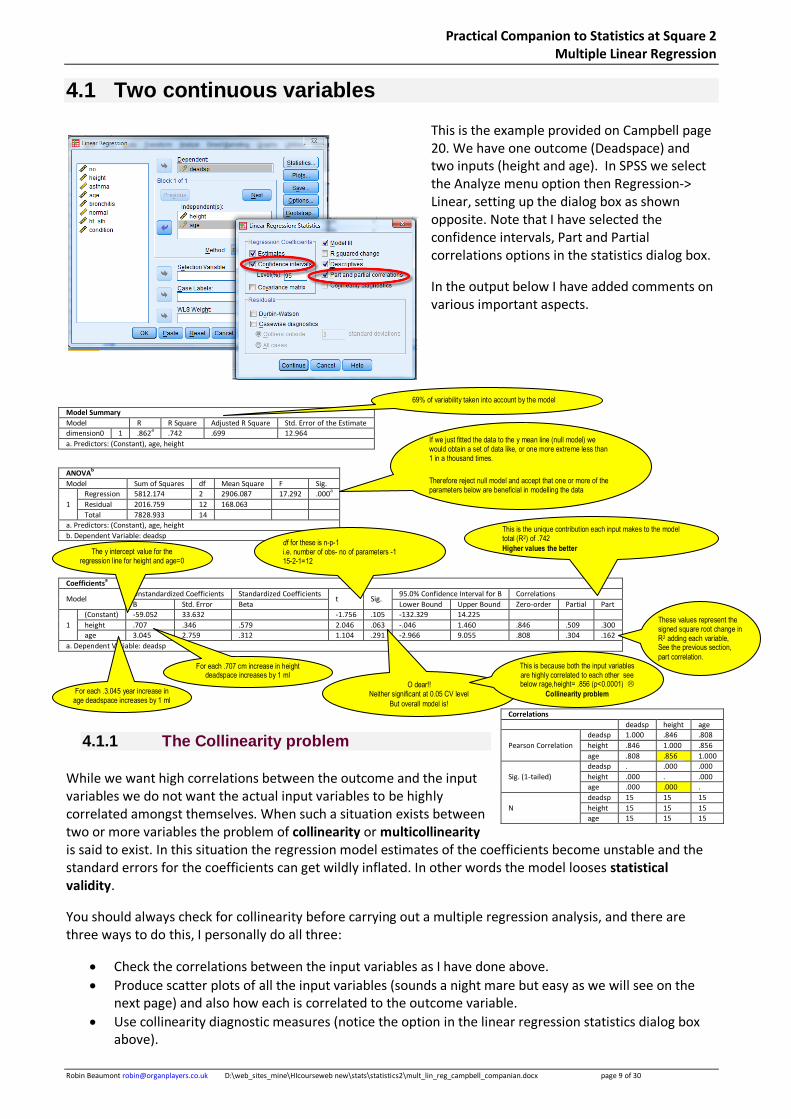
4.1 Two continuous variables

This is the example provided on Campbell page 20. We have one outcome (Deadspace) and two inputs (height and age). In SPSS we select the Analyze menu option then Regression-> Linear, setting up the dialog box as shown opposite. Note that I have selected the confidence intervals, Part and Partial correlations options in the statistics dialog box.

In the output below I have added comments on various important aspects.

Model Summary

Model R R Square Adjusted R Square Std. Error of the Estimate

dimension0 1 .862a .742 .699 12.964

a. Predictors: (Constant), age, height

ANOVA

b

Model Sum of Squares df Mean Square F Sig.

1

Regression 5812.174 2 2906.087 17.292 .000a

Residual 2016.759 12 168.063

Total 7828.933 14

a. Predictors: (Constant), age, height

b. Dependent Variable: deadsp

Coefficients

a

Model Unstandardized Coefficients Standardized Coefficients

t Sig. 95.0% Confidence Interval for B Correlations

B Std. Error Beta Lower Bound Upper Bound Zero-order Partial Part

1

(Constant) -59.052 33.632 -1.756 .105 -132.329 14.225

height .707 .346 .579 2.046 .063 -.046 1.460 .846 .509 .300

age 3.045 2.759 .312 1.104 .291 -2.966 9.055 .808 .304 .162

a. Dependent Variable: deadsp

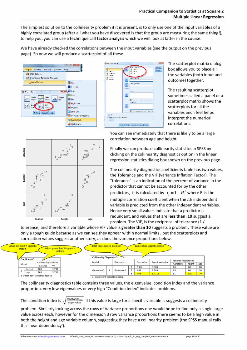
4.1.1 The Collinearity problem

While we want high correlations between the outcome and the input variables we do not want the actual input variables to be highly correlated amongst themselves. When such a situation exists between two or more variables the problem of collinearity or multicollinearity is said to exist. In this situation the regression model estimates of the coefficients become unstable and the standard errors for the coefficients can get wildly inflated. In other words the model looses statistical validity.

You should always check for collinearity before carrying out a multiple regression analysis, and there are three ways to do this, I personally do all three:

Check the correlations between the input variables as I have done above.

Produce scatter plots of all the input variables (sounds a night mare but easy as we will see on the next page) and also how each is correlated to the outcome variable.

Use collinearity diagnostic measures (notice the option in the linear regression statistics dialog box above).

Correlations

deadsp height age

Pearson Correlation

deadsp 1.000 .846 .808

height .846 1.000 .856

age .808 .856 1.000

Sig. (1-tailed)

deadsp . .000 .000

height .000 . .000

age .000 .000 .

N

deadsp 15 15 15

height 15 15 15

age 15 15 15

69% of variability taken into account by the model

If we just fitted the data to the y mean line (null model) we would obtain a set of data like, or one more extreme less than 1 in a thousand times.

Therefore reject null model and accept that one or more of the parameters below are beneficial in modelling the data

For each .707 cm increase in height deadspace increases by 1 ml

For each .3.045 year increase in age deadspace increases by 1 ml

The y intercept value for the regression line for height and age=0

O dear!! Neither significant at 0.05 CV level

But overall model is!

This is because both the input variables are highly correlated to each other see below rage,height= .856 (p<0.0001)

Collinearity problem

This is the unique contribution each input makes to the model total (R2) of .742

Higher values the better

These values represent the signed square root change in R2 adding each variable, See the previous section,

part correlation.

df for these is n-p-1 i.e. number of obs- no of parameters -1 15-2-1=12



The simplest solution to the collinearity problem if it is present, is to only use one of the input variables of a highly correlated group (after all what you have discovered is that the group are measuring the same thing!), to help you, you can use a technique call factor analysis which we will look at latter in the course.

We have already checked the correlations between the input variables (see the output on the previous page). So now we will produce a scatterplot of all these.

The scatterplot matrix dialog box allows you to place all the variables (both input and outcome) together.

The resulting scatterplot sometimes called a panel or a scatterplot matrix shows the scatterplots for all the variables and i feel helps interpret the numerical correlations.

You can see immediately that there is likely to be a large correlation between age and height.

Finally we can produce collinearity statistics in SPSS by clicking on the collinearity diagnostics option in the linear regression statistics dialog box shown on the previous page.

The collinearity diagnostics coefficients table has two values, the Tolerance and the VIF (variance Inflation Factor). The "tolerance" is an indication of the percent of variance in the predictor that cannot be accounted for by the other

predictors, it is calculated by 21i it R where Ri is the

multiple correlation coefficient when the ith independent variable is predicted from the other independent variables. Hence very small values indicate that a predictor is redundant, and values that are less than .10 suggest a problem. The VIF, is the reciprocal of tolerance (1 /

tolerance) and therefore a variable whose VIF value is greater than 10 suggests a problem. These value are only a rough guide because as we can see they appear within normal limits , but the scatterplots and correlation values suggest another story, as does the variance proportions below.

The collinearity diagnostics table contains three values, the eigenvalue, condition index and the variance proportion. very low eigenvalues or very high "Condition Index" indicates problems.

The condition index is max

i

eigenvalue

eigenvalue if this value is large for a specific variable is suggests a collinearity

problem. Similarly looking across the rows of Variance proportions one would hope to find only a single large value across each, however for the dimension 3 row variance proportions there seems to be a high value in both the height and age variable column, suggesting they have a collinearity problem (the SPSS manual calls this 'near dependency').

Coefficientsa

Model Collinearity Statistics

Tolerance VIF

1 height .268 3.731

age .268 3.731


Collinearity Diagnosticsa

Model Dimension Eigenvalue Condition Index Variance Proportions

(Constant) height age

dimension0 1 dimension1

1 2.954 1.000 .00 .00 .00

2 .043 8.269 .09 .00 .30

3 .003 32.111 .91 1.00 .70


Values less than 0.1 suggest a problem

Values greater than 10 suggest a problem

Small values suggest a problem

Large values suggest a problem



Returning once again to the SPSS output on the previous page, we can interpret it using the Venn diagram approach, firstly notice that R2=0.742 this is the total amount of variability that is accounted for by the model (the area in the Venn diagram of all the inputs combined) we can then use the part correlations to see how this is broken down, or alternatively we can work with the sums of squares.

From the above it is clear that age and height share a large amount of the variability (84% worth), my Venn diagram should have very little of age or height which was not overlapping but rather difficult to draw!

Given this finding we would have probably come to much the same conclusion concerning the collinearity problem between age and height if we had just inspected the part correlations in the coefficients table!

4.1.2 Venn diagrams and Correlation equations

We can also relate the above Venn diagrams back to two interesting equations

You can also express the above in the form of various correlation equations, (Howell 2007 p512)

2 2 2 2 2

0.123.. 01 0(2.1) 0(3.12) 0( .123.. 1)...p p pR r r r r

Considering the above example:

This works for which ever input variable you decide to select to use the ordinary correlation value of.

=

.8462

0.7157

+ 0.1622

0.0262

height

0.742

Correlation2 Part

correlation2

age

Multiple R squared Correlation

between outcome + first input

Part correlation between outcome & second input,

controlling for other inputs = + +

Part correlation between outcome & third input,

controlling for other inputs

+ . . . . + Part correlation between

outcome & last input, controlling for other

inputs

0.258 (i.e 1- R2)

0.3002

=.09

height

age

Know total = R2=0.742

Therefore area= 0.742-0.162

2-0.300

2= .6257

0.1622

=.0262

Squared part correlations Sums of squares

2016.759 (residual)

703.2

height

age

2051.7

age common height total

Part correlation2 .0262 .6257 .09 .742

Percentage of total

3.53% 84.32% 12.1% 100%

Sum of squares 2051.69 4899.6 703.27 5812.174

The component sums of squares (yellow) calculated from the regression

sum of squares and using the %'s from the squared part correlations

The 'common' values is not part correlation but useful in the table.

4899.6

<- Both have same proportions ->



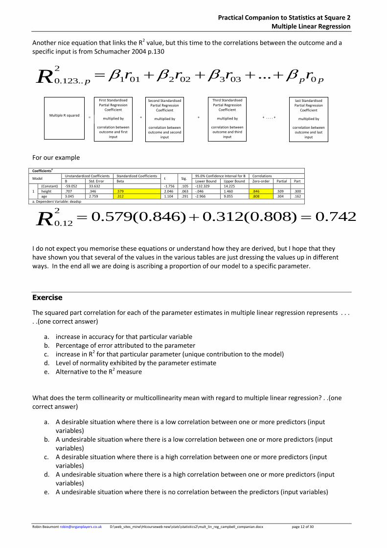
Another nice equation that links the R2 value, but this time to the correlations between the outcome and a specific input is from Schumacher 2004 p.130

2

1 01 2 02 3 03 00.123..... p pp

r r r rR

For our example

Coefficientsa




1

(Constant) -59.052 33.632 -1.756 .105 -132.329 14.225

height .707 .346 .579 2.046 .063 -.046 1.460 .846 .509 .300

age 3.045 2.759 .312 1.104 .291 -2.966 9.055 .808 .304 .162


2

0.120.579(0.846) 0.312(0.808) 0.742R

I do not expect you memorise these equations or understand how they are derived, but I hope that they have shown you that several of the values in the various tables are just dressing the values up in different ways. In the end all we are doing is ascribing a proportion of our model to a specific parameter.

Exercise

The squared part correlation for each of the parameter estimates in multiple linear regression represents . . . . .(one correct answer)

a. increase in accuracy for that particular variable b. Percentage of error attributed to the parameter c. increase in R2 for that particular parameter (unique contribution to the model) d. Level of normality exhibited by the parameter estimate e. Alternative to the R2 measure

What does the term collinearity or multicollinearity mean with regard to multiple linear regression? . .(one correct answer)

a. A desirable situation where there is a low correlation between one or more predictors (input variables)

b. A undesirable situation where there is a low correlation between one or more predictors (input variables)

c. A desirable situation where there is a high correlation between one or more predictors (input variables)

d. A undesirable situation where there is a high correlation between one or more predictors (input variables)

e. A undesirable situation where there is no correlation between the predictors (input variables)

Multiple R squared

First Standardised Partial Regression

Coefficient

multiplied by

correlation between outcome and first

input

= + + + . . . . +

Second Standardised Partial Regression

Coefficient

multiplied by

correlation between outcome and second

input

Third Standardised Partial Regression

Coefficient

multiplied by

correlation between outcome and third

input

last Standardised Partial Regression

Coefficient

multiplied by

correlation between outcome and last

input



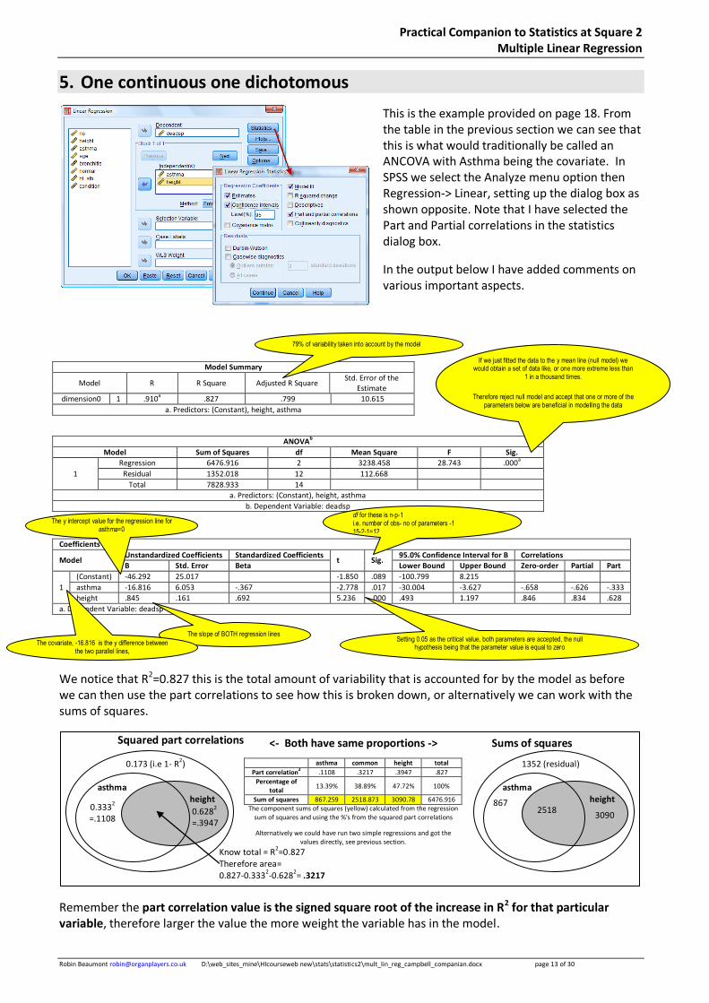
5. One continuous one dichotomous

This is the example provided on page 18. From the table in the previous section we can see that this is what would traditionally be called an ANCOVA with Asthma being the covariate. In SPSS we select the Analyze menu option then Regression-> Linear, setting up the dialog box as shown opposite. Note that I have selected the Part and Partial correlations in the statistics dialog box.

In the output below I have added comments on various important aspects.

Model Summary

Model R R Square Adjusted R Square Std. Error of the

Estimate

dimension0 1 .910a .827 .799 10.615

a. Predictors: (Constant), height, asthma

ANOVAb


1

Regression 6476.916 2 3238.458 28.743 .000a

Residual 1352.018 12 112.668

Total 7828.933 14

a. Predictors: (Constant), height, asthma


Coefficients

a




1

(Constant) -46.292 25.017 -1.850 .089 -100.799 8.215

asthma -16.816 6.053 -.367 -2.778 .017 -30.004 -3.627 -.658 -.626 -.333

height .845 .161 .692 5.236 .000 .493 1.197 .846 .834 .628


We notice that R2=0.827 this is the total amount of variability that is accounted for by the model as before we can then use the part correlations to see how this is broken down, or alternatively we can work with the sums of squares.

Remember the part correlation value is the signed square root of the increase in R2 for that particular variable, therefore larger the value the more weight the variable has in the model.

0.173 (i.e 1- R2)

0.6282

=.3947

height asthma

Know total = R2=0.827

Therefore area= 0.827-0.333

2-0.628

2= .3217

0.3332

=.1108

Squared part correlations Sums of squares

1352 (residual)

3090

height asthma

867

asthma common height total

Part correlation2 .1108 .3217 .3947 .827

Percentage of total

13.39% 38.89% 47.72% 100%

Sum of squares 867.259 2518.873 3090.78 6476.916

The component sums of squares (yellow) calculated from the regression sum of squares and using the %'s from the squared part correlations

Alternatively we could have run two simple regressions and got the values directly, see previous section.

2518

<- Both have same proportions ->

79% of variability taken into account by the model

If we just fitted the data to the y mean line (null model) we would obtain a set of data like, or one more extreme less than

1 in a thousand times.


The slope of BOTH regression lines

The covariate, -16.816 is the y difference between the two parallel lines,

The y intercept value for the regression line for asthma=0

Setting 0.05 as the critical value, both parameters are accepted, the null hypothesis being that the parameter value is equal to zero




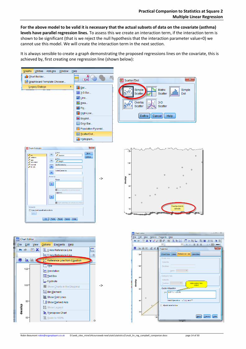
For the above model to be valid it is necessary that the actual subsets of data on the covariate (asthma) levels have parallel regression lines. To assess this we create an interaction term, if the interaction term is shown to be significant (that is we reject the null hypothesis that the interaction parameter value=0) we cannot use this model. We will create the interaction term in the next section.

It is always sensible to create a graph demonstrating the proposed regressions lines on the covariate, this is achieved by, first creating one regression line (shown below):

->

->



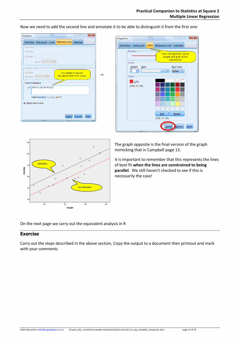
Now we need to add the second line and annotate it to be able to distinguish it from the first one:

->

The graph opposite is the final version of the graph mimicking that in Campbell page 13.

It is important to remember that this represents the lines of best fit when the lines are constrained to being parallel. We still haven't checked to see if this is necessarily the case!

On the next page we carry out the equivalent analysis in R

Exercise

Carry out the steps described in the above section, Copy the output to a document then printout and mark with your comments

asthmatics

non-asthmatics



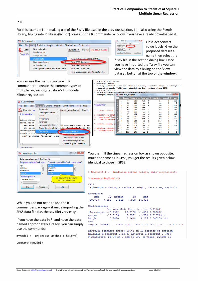
In R

For this example I am making use of the *.sav file used in the previous section. I am also using the Rcmdr library, typing into R, library(Rcmdr) brings up the R commander window if you have already downloaded it.

Unselect convert value labels. Give the proposed dataset a name then select the

*.sav file in the section dialog box. Once you have imported the *.sav file you can view the data by clicking on the 'view dataset' button at the top of the window:

You can use the menu structure in R commander to create the common types of multiple regression,statistics-> Fit models->linear regression:

You then fill the Linear regression box as shown opposite, much the same as in SPSS, you get the results given below, identical to those in SPSS.

While you do not need to use the R commander package – it made importing the SPSS data file (i.e. the sav file) very easy.

If you have the data in R, and have the data named appropriately already, you can simply use the commands:

mymodel <- Im(deadsp~asthma + height)

summary(mymodel)



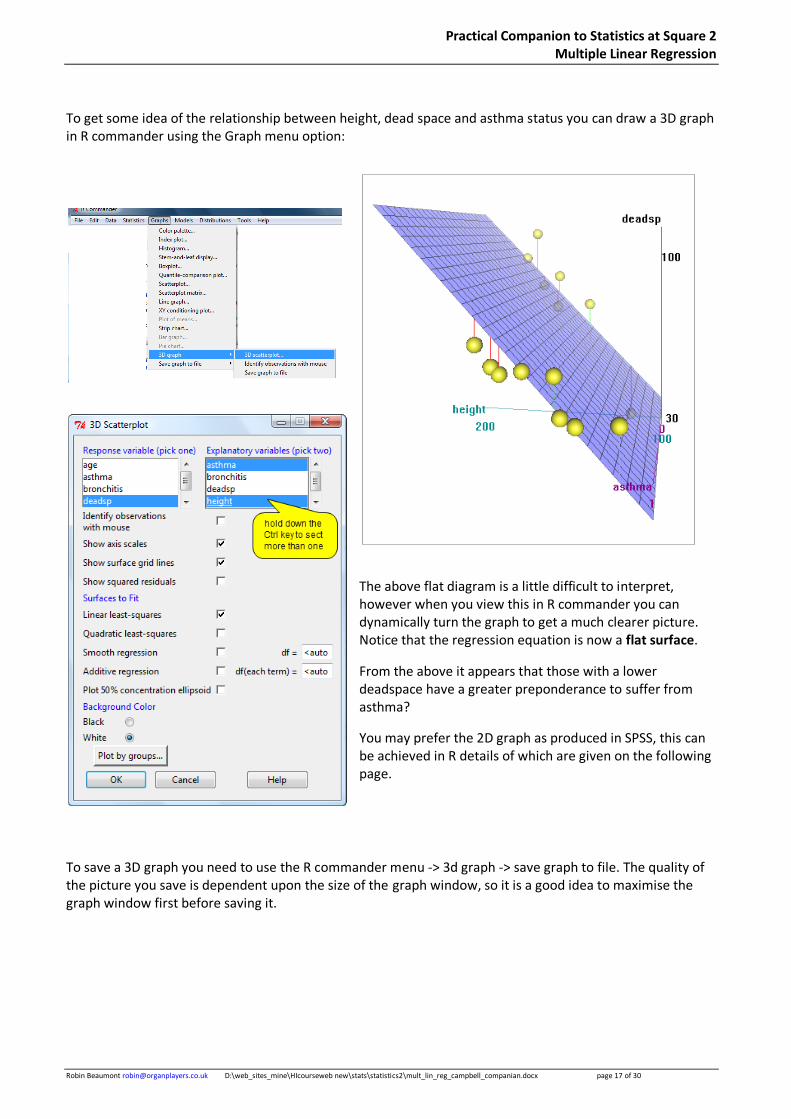
To get some idea of the relationship between height, dead space and asthma status you can draw a 3D graph in R commander using the Graph menu option:

The above flat diagram is a little difficult to interpret, however when you view this in R commander you can dynamically turn the graph to get a much clearer picture. Notice that the regression equation is now a flat surface.

From the above it appears that those with a lower deadspace have a greater preponderance to suffer from asthma?

You may prefer the 2D graph as produced in SPSS, this can be achieved in R details of which are given on the following page.

To save a 3D graph you need to use the R commander menu -> 3d graph -> save graph to file. The quality of the picture you save is dependent upon the size of the graph window, so it is a good idea to maximise the graph window first before saving it.



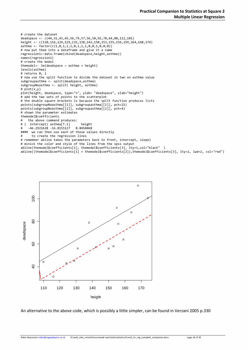
# create the dataset deadspace <- c(44,31,43,45,56,79,57,56,58,92,78,64,88,112,101) height <- c(110,116,124,129,131,138,142,150,153,155,156,159,164,168,174) asthma <- factor(c(1,0,1,1,1,0,1,1,1,0,0,1,0,0,0)) # now put them into a dataframe and give it a name regression1<-data.frame(cbind(deadspace,height,asthma)) names(regression1) # create the model themodel<- lm(deadspace ~ asthma + height) levels(asthma) # returns 0, 1 # now use the split function to divide the dataset in two on asthma value subgroupasthma <- split(deadspace,asthma) subgroupNoasthma <- split( height, asthma) # plot(x,y) plot(height, deadspace, type="n", ylab= "deadspace", xlab="height") # add the two sets of points to the scatterplot # the double square brackets is because the split function produces lists points(subgroupNoasthma[[1]], subgroupasthma[[1]], pch=21) points(subgroupNoasthma[[2]], subgroupasthma[[2]], pch=4) # shown the parameter estimates themodel$coefficients # the above command produces: # ( Intercept) asthma[T.1] height # -46.2921628 -16.8155127 0.8450468 #### we can then use each of these values directly # to create the regression lines # remember abline takes the parameters back to front, intercept, slope) # minick the color and style of the lines from the spss output abline(themodel$coefficients[1], themodel$coefficients[3], lty=1,col="black" ) abline((themodel$coefficients[1] + themodel$coefficients[2]),themodel$coefficients[3], lty=2, lwd=2, col="red")

An alternative to the above code, which is possibly a little simpler, can be found in Verzani 2005 p.330

110 120 130 140 150 160 170

40

60

80

10

0

height

de

ad

sp

ace



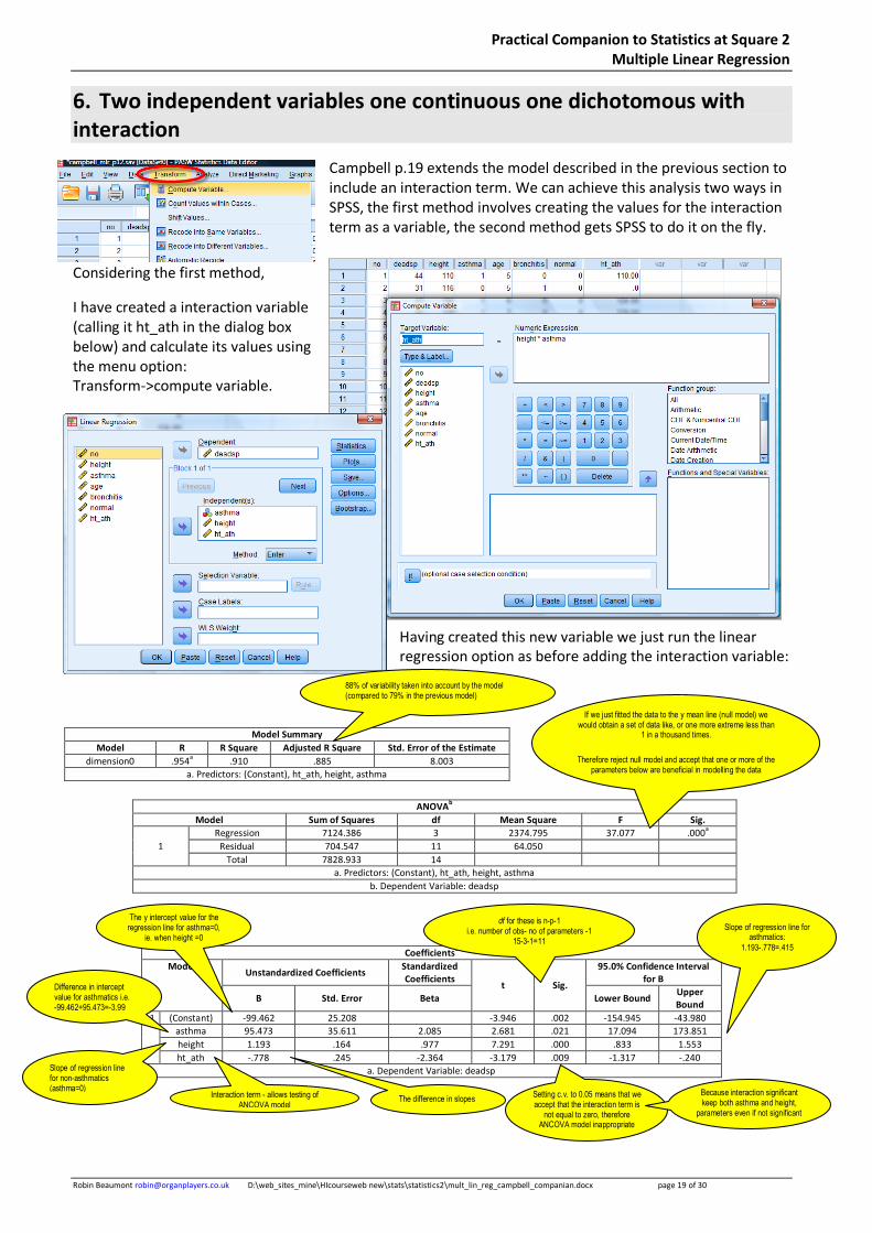
6. Two independent variables one continuous one dichotomous with interaction

Campbell p.19 extends the model described in the previous section to include an interaction term. We can achieve this analysis two ways in SPSS, the first method involves creating the values for the interaction term as a variable, the second method gets SPSS to do it on the fly.

Considering the first method,

I have created a interaction variable (calling it ht_ath in the dialog box below) and calculate its values using the menu option: Transform->compute variable.

Having created this new variable we just run the linear regression option as before adding the interaction variable:

Model Summary

Model R R Square Adjusted R Square Std. Error of the Estimate

dimension0 .954a .910 .885 8.003

a. Predictors: (Constant), ht_ath, height, asthma

Coefficientsa

Model Unstandardized Coefficients

Standardized Coefficients

t Sig.

95.0% Confidence Interval for B

B Std. Error Beta Lower Bound Upper Bound

1 (Constant) -99.462 25.208 -3.946 .002 -154.945 -43.980

asthma 95.473 35.611 2.085 2.681 .021 17.094 173.851

height 1.193 .164 .977 7.291 .000 .833 1.553

ht_ath -.778 .245 -2.364 -3.179 .009 -1.317 -.240


ANOVAb


1

Regression 7124.386 3 2374.795 37.077 .000a

Residual 704.547 11 64.050

Total 7828.933 14

a. Predictors: (Constant), ht_ath, height, asthma


88% of variability taken into account by the model (compared to 79% in the previous model)

If we just fitted the data to the y mean line (null model) we would obtain a set of data like, or one more extreme less than

1 in a thousand times.


The difference in slopes Interaction term - allows testing of

ANCOVA model

Setting c.v. to 0.05 means that we accept that the interaction term is

not equal to zero, therefore ANCOVA model inappropriate

Difference in intercept value for asthmatics i.e. -99.462+95.473=-3.99

The y intercept value for the regression line for asthma=0,

ie. when height =0

Slope of regression line for non-asthmatics (asthma=0)

Slope of regression line for asthmatics:

1.193-.778=.415

Because interaction significant keep both asthma and height,

parameters even if not significant

df for these is n-p-1 i.e. number of obs- no of parameters -1

15-3-1=11



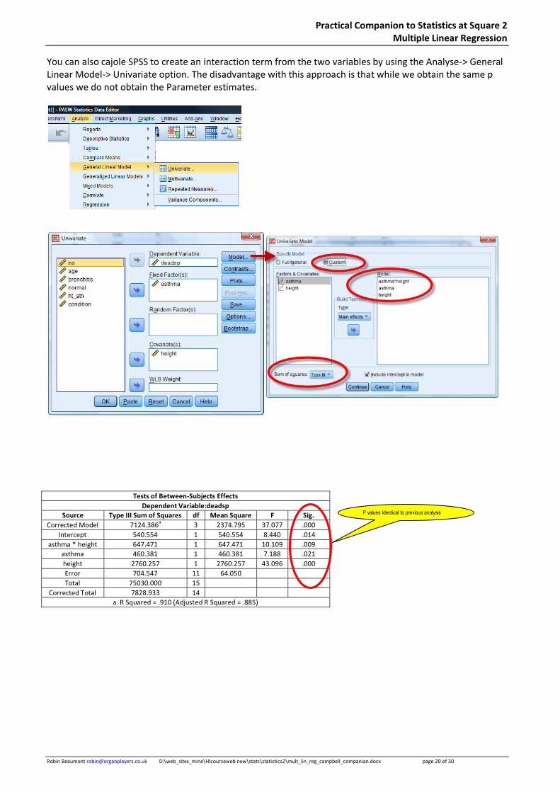
You can also cajole SPSS to create an interaction term from the two variables by using the Analyse-> General Linear Model-> Univariate option. The disadvantage with this approach is that while we obtain the same p values we do not obtain the Parameter estimates.

Tests of Between-Subjects Effects

Dependent Variable:deadsp

Source Type III Sum of Squares df Mean Square F Sig.

Corrected Model 7124.386a 3 2374.795 37.077 .000

Intercept 540.554 1 540.554 8.440 .014

asthma * height 647.471 1 647.471 10.109 .009

asthma 460.381 1 460.381 7.188 .021

height 2760.257 1 2760.257 43.096 .000

Error 704.547 11 64.050

Total 75030.000 15

Corrected Total 7828.933 14

a. R Squared = .910 (Adjusted R Squared = .885)

P values Identical to previous analysis



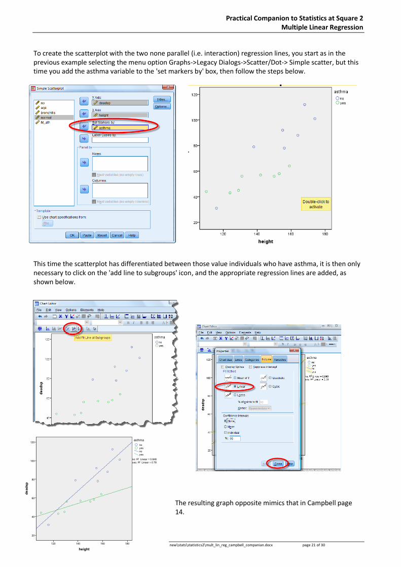
To create the scatterplot with the two none parallel (i.e. interaction) regression lines, you start as in the previous example selecting the menu option Graphs->Legacy Dialogs->Scatter/Dot-> Simple scatter, but this time you add the asthma variable to the 'set markers by' box, then follow the steps below.

This time the scatterplot has differentiated between those value individuals who have asthma, it is then only necessary to click on the 'add line to subgroups' icon, and the appropriate regression lines are added, as shown below.

The resulting graph opposite mimics that in Campbell page 14.



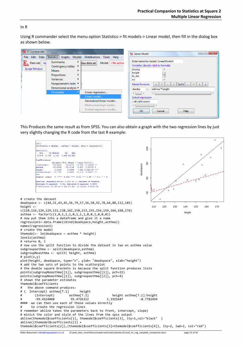
In R

Using R commander select the menu option Statistics-> fit models-> Linear model, then fill in the dialog box as shown below.

This Produces the same result as from SPSS. You can also obtain a graph with the two regression lines by just very slightly changing the R code from the last R example:

# create the dataset deadspace <- c(44,31,43,45,56,79,57,56,58,92,78,64,88,112,101) height <- c(110,116,124,129,131,138,142,150,153,155,156,159,164,168,174) asthma <- factor(c(1,0,1,1,1,0,1,1,1,0,0,1,0,0,0)) # now put them into a dataframe and give it a name regression1<-data.frame(cbind(deadspace,height,asthma)) names(regression1) # create the model themodel<- lm(deadspace ~ asthma * height) levels(asthma) # returns 0, 1 # now use the split function to divide the dataset in two on asthma value subgroupasthma <- split(deadspace,asthma) subgroupNoasthma <- split( height, asthma) # plot(x,y) plot(height, deadspace, type="n", ylab= "deadspace", xlab="height") # add the two sets of points to the scatterplot # the double square brackets is because the split function produces lists points(subgroupNoasthma[[1]], subgroupasthma[[1]], pch=21) points(subgroupNoasthma[[2]], subgroupasthma[[2]], pch=4) # shown the parameter estimates themodel$coefficients # the above command produces: # ( Intercept) asthma[T.1] height # (Intercept) asthma[T.1] height asthma[T.1]:height # -99.4624060 95.4726312 1.1925647 -0.7782494 #### we can then use each of these values directly # to create the regression lines # remember abline takes the parameters back to front, intercept, slope) # minick the color and style of the lines from the spss output abline(themodel$coefficients[1], themodel$coefficients[3], lty=1,col="black" ) abline((themodel$coefficients[1] + themodel$coefficients[2]),(themodel$coefficients[3]+themodel$coefficients[4]), lty=2, lwd=2, col="red")

110 120 130 140 150 160 170

40

60

80

10

0

height

de

ad

sp

ace



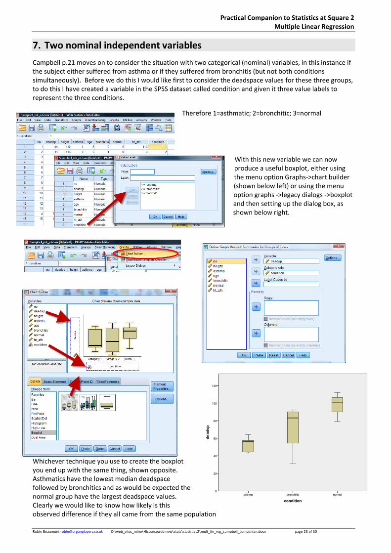
7. Two nominal independent variables

Campbell p.21 moves on to consider the situation with two categorical (nominal) variables, in this instance if the subject either suffered from asthma or if they suffered from bronchitis (but not both conditions simultaneously). Before we do this I would like first to consider the deadspace values for these three groups, to do this I have created a variable in the SPSS dataset called condition and given it three value labels to represent the three conditions.

Therefore 1=asthmatic; 2=bronchitic; 3=normal

With this new variable we can now produce a useful boxplot, either using the menu option Graphs->chart builder (shown below left) or using the menu option graphs ->legacy dialogs ->boxplot and then setting up the dialog box, as shown below right.

Whichever technique you use to create the boxplot you end up with the same thing, shown opposite. Asthmatics have the lowest median deadspace followed by bronchitics and as would be expected the normal group have the largest deadspace values. Clearly we would like to know how likely is this observed difference if they all came from the same population



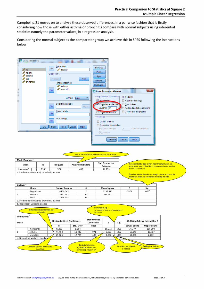
Campbell p.21 moves on to analyse these observed differences, in a pairwise fashion that is firstly considering how those with either asthma or bronchitis compare with normal subjects using inferential statistics namely the parameter values, in a regression analysis.

Considering the normal subject as the comparator group we achieve this in SPSS following the instructions below.

Model Summary


Estimate

dimension0 1 .755a .571 .499 16.739

a. Predictors: (Constant), bronchitis, asthma

ANOVA

b


1

Regression 4466.642 2 2233.321 7.971 .006a

Residual 3362.292 12 280.191

Total 7828.933 14

a. Predictors: (Constant), bronchitis, asthma


Coefficients

a

Model Unstandardized Coefficients

Standardized Coefficients t Sig.

95.0% Confidence Interval for B


1

(Constant) 97.333 9.664 10.072 .000 76.277 118.390

asthma -44.458 11.332 -.971 -3.923 .002 -69.149 -19.767

bronchitis -25.083 12.785 -.486 -1.962 .073 -52.938 2.772


49% of the variability is taken into account by the model

If we just fitted the data to the y mean line (null model) we would obtain a set of data like, or one more extreme, less than 6 times in a thousand.


Conclude Asthmatics significantly different from normals as p values < C.V

Difference between normals and asthmatics

Setting C.V. to 0.05 Difference between normals and bronchitics

Bronchitics not different to normals




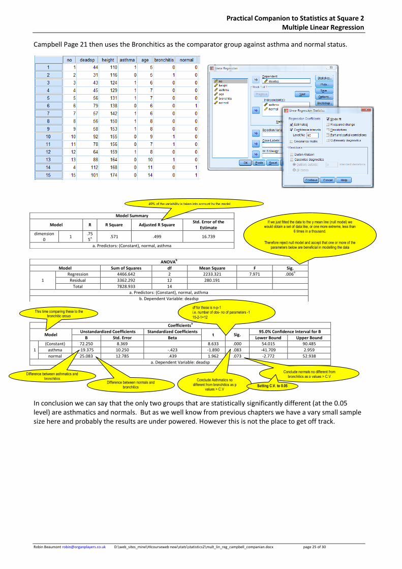
Campbell Page 21 then uses the Bronchitics as the comparator group against asthma and normal status.

Coefficientsa


t Sig. 95.0% Confidence Interval for B


1

(Constant) 72.250 8.369 8.633 .000 54.015 90.485

asthma -19.375 10.250 -.423 -1.890 .083 -41.709 2.959

normal 25.083 12.785 .439 1.962 .073 -2.772 52.938


In conclusion we can say that the only two groups that are statistically significantly different (at the 0.05 level) are asthmatics and normals. But as we well know from previous chapters we have a vary small sample size here and probably the results are under powered. However this is not the place to get off track.

Model Summary


Estimate

dimension0

1 .755

a

.571 .499 16.739

a. Predictors: (Constant), normal, asthma

ANOVAb


1

Regression 4466.642 2 2233.321 7.971 .006a

Residual 3362.292 12 280.191

Total 7828.933 14

a. Predictors: (Constant), normal, asthma


49% of the variability is taken into account by the model (compared to 79% in the previous model

Conclude Asthmatics no different from bronchitics as p

values > C.V

This time comparing these to the bronchitic group

Difference between asthmatics and bronchitics

49% of the variability is taken into account by the model

If we just fitted the data to the y mean line (null model) we would obtain a set of data like, or one more extreme, less than

6 times in a thousand.


Difference between normals and bronchitics

Conclude normals no different from bronchitics as p values > C.V

Setting C.V. to 0.05

df for these is n-p-1 i.e. number of obs- no of parameters -1

15-2-1=12



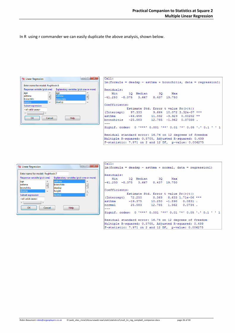
In R using r commander we can easily duplicate the above analysis, shown below.



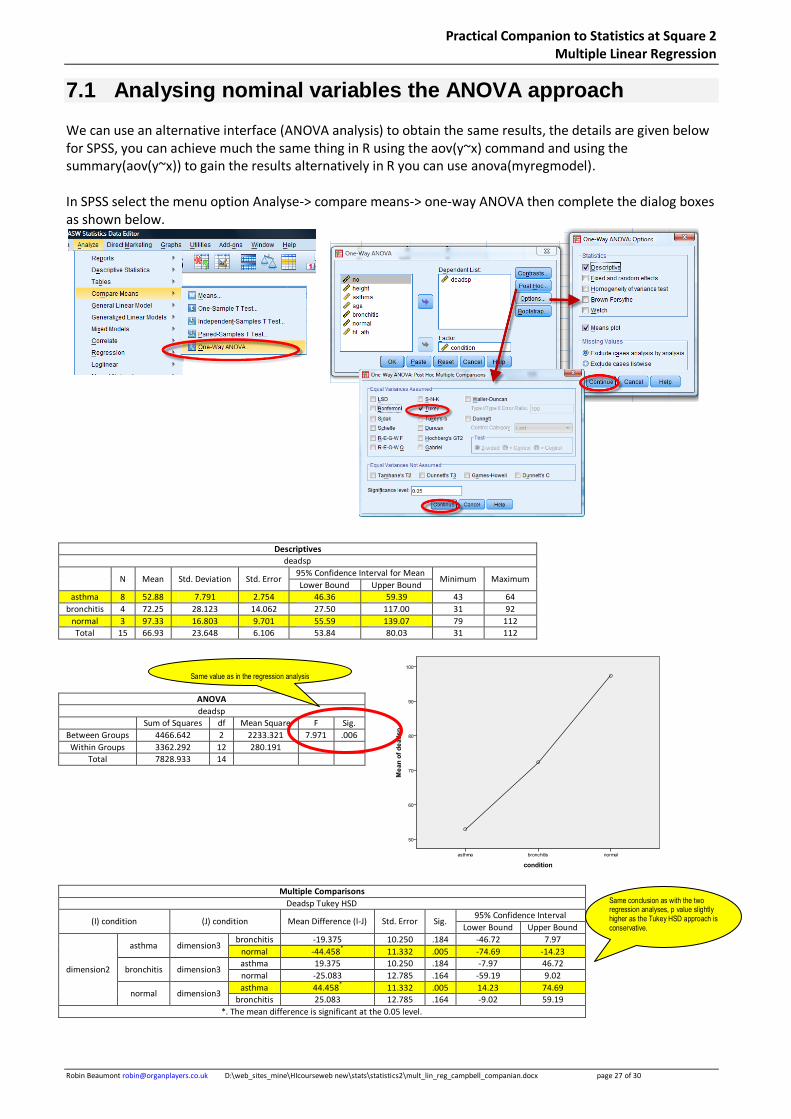
7.1 Analysing nominal variables the ANOVA approach

We can use an alternative interface (ANOVA analysis) to obtain the same results, the details are given below for SPSS, you can achieve much the same thing in R using the aov(y~x) command and using the summary(aov(y~x)) to gain the results alternatively in R you can use anova(myregmodel). In SPSS select the menu option Analyse-> compare means-> one-way ANOVA then complete the dialog boxes as shown below.

Descriptives

deadsp

N Mean Std. Deviation Std. Error 95% Confidence Interval for Mean

Minimum Maximum Lower Bound Upper Bound

asthma 8 52.88 7.791 2.754 46.36 59.39 43 64

bronchitis 4 72.25 28.123 14.062 27.50 117.00 31 92

normal 3 97.33 16.803 9.701 55.59 139.07 79 112

Total 15 66.93 23.648 6.106 53.84 80.03 31 112

ANOVA

deadsp

Sum of Squares df Mean Square F Sig.

Between Groups 4466.642 2 2233.321 7.971 .006

Within Groups 3362.292 12 280.191

Total 7828.933 14

Multiple Comparisons

Deadsp Tukey HSD

(I) condition (J) condition Mean Difference (I-J) Std. Error Sig. 95% Confidence Interval

Lower Bound Upper Bound

dimension2

asthma dimension3 bronchitis -19.375 10.250 .184 -46.72 7.97

normal -44.458* 11.332 .005 -74.69 -14.23

bronchitis dimension3 asthma 19.375 10.250 .184 -7.97 46.72

normal -25.083 12.785 .164 -59.19 9.02

normal dimension3 asthma 44.458

* 11.332 .005 14.23 74.69

bronchitis 25.083 12.785 .164 -9.02 59.19

*. The mean difference is significant at the 0.05 level.

Same value as in the regression analysis

Same conclusion as with the two regression analyses, p value slightly higher as the Tukey HSD approach is conservative.



8. Assumptions, Residuals, leverage and influence

Campbell summarises these issues well in the chapter, and we visited the practicalities checking these aspects in the chapter on simple linear regression analysis I suggest you revisit that chapter now.

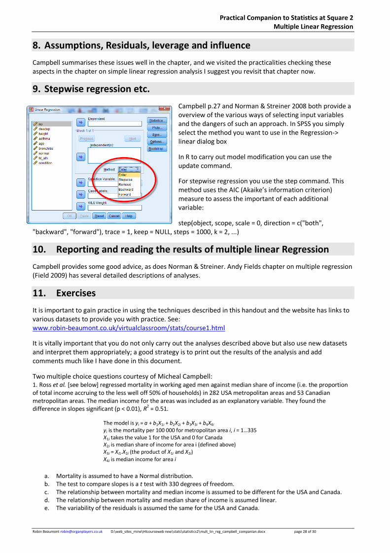
9. Stepwise regression etc.

Campbell p.27 and Norman & Streiner 2008 both provide a overview of the various ways of selecting input variables and the dangers of such an approach. In SPSS you simply select the method you want to use in the Regression-> linear dialog box

In R to carry out model modification you can use the update command.

For stepwise regression you use the step command. This method uses the AIC (Akaike’s information criterion) measure to assess the important of each additional variable:

step(object, scope, scale = 0, direction = c("both", "backward", "forward"), trace = 1, keep = NULL, steps = 1000, k = 2, ...)

10. Reporting and reading the results of multiple linear Regression

Campbell provides some good advice, as does Norman & Streiner. Andy Fields chapter on multiple regression (Field 2009) has several detailed descriptions of analyses.

11. Exercises

It is important to gain practice in using the techniques described in this handout and the website has links to various datasets to provide you with practice. See: www.robin-beaumont.co.uk/virtualclassroom/stats/course1.html

It is vitally important that you do not only carry out the analyses described above but also use new datasets and interpret them appropriately; a good strategy is to print out the results of the analysis and add comments much like I have done in this document.

Two multiple choice questions courtesy of Micheal Campbell: 1. Ross et al. [see below] regressed mortality in working aged men against median share of income (i.e. the proportion of total income accruing to the less well off 50% of households) in 282 USA metropolitan areas and 53 Canadian metropolitan areas. The median income for the areas was included as an explanatory variable. They found the difference in slopes significant (p < 0.01), R2 = 0.51.

The model is yi = a + b1X1i + b2X2i + b3X3i + b4X4i yi is the mortality per 100 000 for metropolitan area i, i = 1…335 X1i takes the value 1 for the USA and 0 for Canada X2i is median share of income for area i (defined above) X3i = Xi1.X2i (the product of X1i and X2i) X4i is median income for area i

a. Mortality is assumed to have a Normal distribution. b. The test to compare slopes is a t test with 330 degrees of freedom. c. The relationship between mortality and median income is assumed to be different for the USA and Canada. d. The relationship between mortality and median share of income is assumed linear. e. The variability of the residuals is assumed the same for the USA and Canada.




Ross NA, Wolfson MC, Dunn JR, Berthelot J-M, Kaplan GA, Lynch JW. Relation between income inequality and mortality in Canada and in the United States: cross-sectional assessment using census data and vital statistics. BMJ 2000; 320: 898–902

2. In a multiple regression equation y = a + b1X1 + b2X2,

a. The independent’ variables X1 and X2 must be continuous b. The leverage depends on the values of y. c. The slope b2 is unaffected by values of X1. d. If X2 is a categorical variable with three categories, it is modelled by two dummy variables. e. If there are 100 points in the data set, then there are 97 degrees of freedom for testing b1.

12. Summary

This chapter was concerned with the practicalities of carrying out multiple linear regression in both SPSS and R and the appropriate interpretation of the results. It introduced the Venn diagram interpretation and described how various part correlations and sums of squares were equivalent in interpreting the unique contribution each predictor (i.e. input) variable makes to the model.

While this practical guide did not dwell on residual analysis as was the case in my Simple regression chapter – this process is still as important in multiple linear regression, you just apply the same techniques as described in that chapter again.

It is suggested that you now re-read the Linear regression chapter in Campbell' statistics at square two as a resume.



13. References

Campbell M 2006 (2nd ed.) Statistics at square two. BMJ books – Blackwell publishing.

Crawley M J 2005 Statistics: An introduction using R. Wiley

Daniel W W 1991 Biostatistics: A foundation for analysis in the health sciences. Wiley.

Field A 2009 Discovering Statistics Using SPSS. Sage

Howell D C 2006 Statistical Methods for Psychology (Ise) (Paperback)

Miles J, Shevlin M 2001 Applying regression & correlation: A guide for students and researchers. Sage publications. London

Norman G R, Streiner D L. 2008 (3rd ed) Biostatistics: The bare Essentials.

Shumacher R E Lomax R G 2004 A beginners guide to structural equation modelling. Lawrence Erlbaum.

Advanced reading:

Scheffe H 1999 (reprint of the 1959 edition) The analysis of variance. Wiley-IEEE

Cohen, J., Cohen P., West, S.G., & Aiken, L.S. 2003 Applied multiple regression/correlation analysis for the behavioral sciences. (3rd ed.) Hillsdale, NJ: Lawrence Erlbaum Associates.

14. Appendix - Some graphical options in R

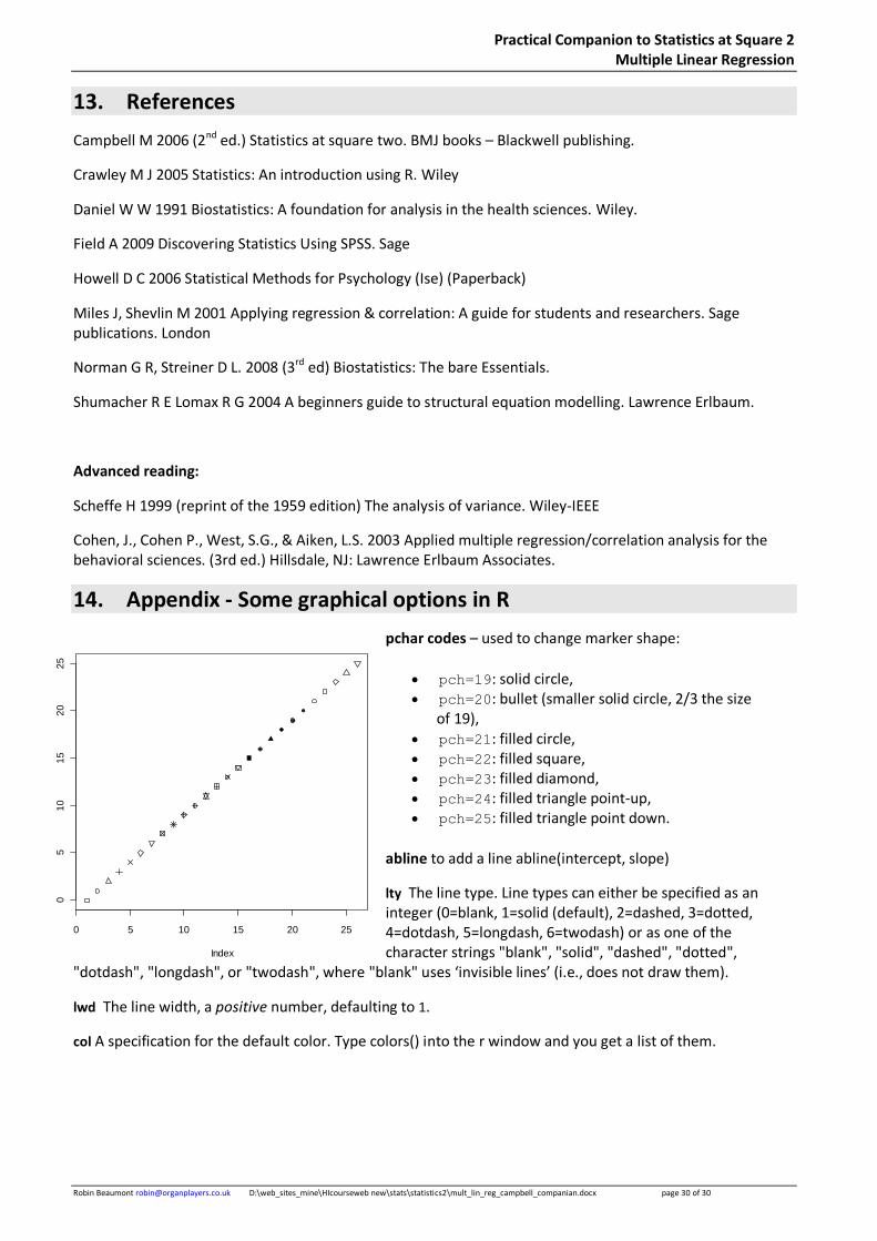
pchar codes – used to change marker shape:

pch=19: solid circle, pch=20: bullet (smaller solid circle, 2/3 the size

of 19), pch=21: filled circle, pch=22: filled square, pch=23: filled diamond, pch=24: filled triangle point-up, pch=25: filled triangle point down.

abline to add a line abline(intercept, slope)

lty The line type. Line types can either be specified as an integer (0=blank, 1=solid (default), 2=dashed, 3=dotted, 4=dotdash, 5=longdash, 6=twodash) or as one of the character strings "blank", "solid", "dashed", "dotted",

"dotdash", "longdash", or "twodash", where "blank" uses ‘invisible lines’ (i.e., does not draw them).

lwd The line width, a positive number, defaulting to 1.

col A specification for the default color. Type colors() into the r window and you get a list of them.

0 5 10 15 20 25

05

10

15

20

25

Index

0:2

5

Documents

multiple linear regression - floppybunny.org · Practical Companion to Statistics at Square 2 Multiple Linear Regression Robin Beaumont [email protected] D:\web_sites_mine\HIcourseweb