DPRIETI Discussion Paper Series 16-E-030

Multiple Lenders, Temporary Debt Restructuring, andFirm Performance: Evidence from contract-level data

MIYAKAWA DaisukeHitotsubashi University

OHASHI KazuhikoHitotsubashi University

The Research Institute of Economy, Trade and Industryhttp://www.rieti.go.jp/en/

1

RIETI Discussion Paper Series 16-E-030

March 2016

Multiple Lenders, Temporary Debt Restructuring, and Firm Performance: Evidence from contract-level data*

MIYAKAWA Daisuke

Hitotsubashi University

OHASHI Kazuhiko

Hitotsubashi University

Abstract

This paper empirically examines the cause and consequence of private debt restructurings out of court. Using

unique contract-level data accounting for Japanese bank loans, we employ probit and multinomial logit

estimations to study how demand and approval of debt restructuring are determined, as well as under what

conditions one specific form of debt restructuring—temporary debt restructuring—is utilized. The results of our

estimations show, first, that the demand of debt restructuring is systematically associated with firm

characteristics and the relation-specific characteristics. Second, debt restructurings are more likely to take a

“temporary” form when the number of lender banks is larger. Using propensity score matching

difference-in-difference estimation, we further find that the performance of firms experiencing temporary debt

restructuring significantly deteriorates in comparison with that of firms experiencing non-temporary debt

restructuring. Furthermore, such pattern is more likely to be observed when lender banks have weaker balance

sheet conditions. These results imply that temporary debt restructuring during our sample period was mainly

used as de facto evergreening lending, which ended up deteriorating borrower creditworthiness.

Keywords: Debt restructuring, Number of banks, Firm performance, Evergreening lending

JEL classification: G21, G32, K12, L14, D82

RIETI Discussion Papers Series aims at widely disseminating research results in the form of professional

papers, thereby stimulating lively discussion. The views expressed in the papers are solely those of the

author(s), and neither represent those of the organization to which the author(s) belong(s) nor the Research

Institute of Economy, Trade and Industry.

*This research was conducted as a part of the Research Institute of Economy, Trade and Industry (RIETI) researchproject “Study on Corporate Finance and Firm Dynamics.” We would like to thank Iichiro Uesugi, Kaoru Hosono,Arito Ono, Hirofumi Uchida, Masazumi Hattori, Xu Peng, Wako Watanabe, Toshihiro Okubo, Mathias Hoffman,Miho Takizawa, Hiroshi Ohashi, Masahisa Fujita, Masayuki Morikawa, Atsushi Nakajima, and participants ofseminars at the Research Institute of Economy, Trade and Industry (RIETI). This study utilizes the micro data of thequestionnaire information based on the firm-level survey data collected on October 2014 in Japan by ResearchInstitute of Economy, Trade and Industry for the study of the impact associated with the termination of the SMEfinancial act.

2

1. Introduction Private debt restructuring including the postponement of debt repayment, which is often

employed for renegotiating bank loan (Roberts and Sufi 2008; Roberts 2015), has the similar economic role to the provision of additional loan in the sense that both provide borrowers the benefit of time associated with loan repayment. In spite of such importance of debt restructuring as a financial tool, however, our knowledge on the cause and consequence of debt restructuring – in particular that between banks and unlisted firms – is still limited mainly due to the lack of reliable contract-level data on private debt restructuring. It is not straightforward to collect the information associated with private debt restructuring out of court even for listed firms since publicly available information (e.g., financial statement) could not fully account for the exact contents of debt restructuring. Furthermore, it becomes almost impossible to systematically collect the information associated with the private debt renegotiation between banks and unlisted firms, for which even the financial statement is not generally publicly available.

Reflecting the limitation of such data availability, the extant studies on the cause of debt restructuring have relied on hand-picked data. Roberts and Sufi (2008), for example, use the data for 1,000 U.S. public firms augmented by hand-picked data accounting for various debt contract modifications. 4 Bruner and Krahnen (2008) also employ the distressed corporate debtors’ information consists of 124 borrower firms, which is directly obtained from six major German banks’ internal information. Although these recent studies have certainly opened up the empirical analyses on the cause of debt restructuring, contract-level empirical evidence is still comparatively scarce.

Against this background, the first motivation of the present paper is to study the cause of private debt restructuring by using a novel dataset accounting for more than 5,000 unlisted firms, among which around 1,500 firms experienced private debt restructuring out of court. The dataset is compiled from the survey data conducted on October 2014 for Japanese unlisted firms and contain wide variety of firm-specific, bank-specific, and firm-bank relationship-specific characteristics as well as the detailed information on the contents of debt restructuring. Distinct from the extant studies exclusively focusing on the characteristics of firms experiencing debt restructuring, the present study starts its analysis from the discussion on the determinants of demand for debt restructuring. Then, controlling for such demand, we further study the determinants of the approval for debt restructuring. This could be possible because using the abovementioned dataset, we can identify firms requesting renegotiation and approved, requesting but rejected, and not requesting. As far as we concern, there is no extant study employing the data with such wide coverage and detailed information associated with debt restructuring.

4 Denis and Wang (2014) also employ the data set obtaining from the same data source.

3

Apart from the studies on the cause of debt restructuring, a number of extant studies have also been paying an attention to the consequence of debt restructuring. As a prominent study, for example, Gilson et al. (1990) employs event study approach to examine the impact associated with listed companies’ debt-relief request. Following the same methodological framework, Inoue et al. (2008) and Godlewski (2015) revisit the same question and show that further detailed features of debt restructuring (e.g., who led the restructuring, what role financial authorities’ bank supervision played, how frequent renegotiation occurred, etc.) matter in terms of the economic impact of private debt renegotiation. Here, we should note that all of these extant studies exclusively focus on firms’ stock price under event study framework, and thus examine only the listed companies. Against this background, the second motivation of the present paper is to extend the analysis on the consequence of debt restructuring both toward the one including unlisted firms and the one employing other measures for firm performance than stock prices (i.e., firms’ financial statement information).

From the theoretical point of view, as discussed in the classical paper (e.g., Bolton and Scharfstein 1996; Dewatripont and Maskin 1995), larger number of lender banks is presumed to make it harder for related parties to renegotiate debt. According to their discussion, such a restriction on debt restructuring originated from the dispersed banks relations is used to effectively induce borrowers to appropriately behave. Despite the simple prediction that the difficulty of debt restructuring is positively correlated with the number of lender banks, which is provided by these theoretical models, empirically examining how the number of lender banks affects the probability of debt renegotiation is not straightforward. This is mainly because we need to identify whether firms actually request for debt restructuring, whether firms apply for the debt restructuring, and whether such application is approved or not. These information is necessary to avoid the endogeneity bias associated with the omitted variables such as firms’ demand for debt restructuring. As already mentioned, the data we use in the present paper includes all the information we need to test the prediction in the abovementioned classical paper. This leads to the third motivation of this paper that empirically tests it.

As mentioned at the outset, debt restructuring, especially that includes the postponement of debt repayment, shares the same feature with loan provision as both provide borrowers the benefit of time to repay. This means that a bust amount of extant literature on bank lending are largely related to the discussion on debt restructuring. Among those extant studies, we aim to link the present paper to one research issue – banks’ provision of evergreening loan. As an illustration, Peek and Rosengren (2005) point out that Japanese banks had a perverse incentive to provide additional loan to the weakest borrower in order to avoid the realization of losses on their balance sheet. Given the fact that our dataset contains various firm characteristics including performance measures, we can

4

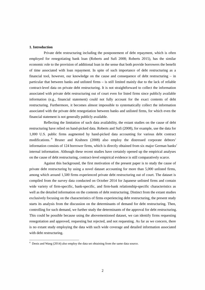
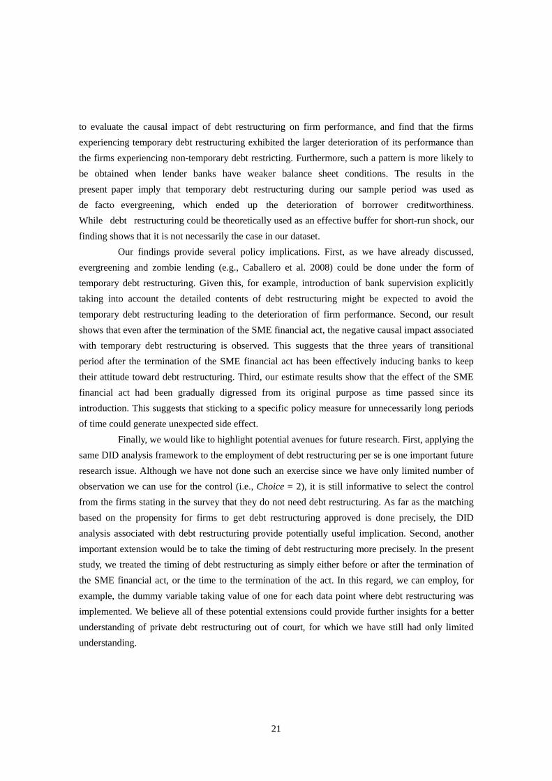
explicitly study for what type of firms banks grant debt restructuring, and what the impact of the restructuring on firm performance in the context of evergreening. In this regard, we are specifically interested in whether the conducted debt restructuring is “temporary” fashion or not. Such temporary debt restructuring is typically observed in the form that repayment schedule is modified over short periods (e.g., within one year) without reducing principal or interests. Under this modification, it is certain for firms and lender banks to renegotiate again in near future since it is highly difficult for borrower firms to repay the debt under such modified schedule unless firms face good windfall (see Figure 1). We presume that this type of temporary debt restructuring shares the same economic feature with the provision of evergreening loan since such debt restructuring could be done to avoid the realization of losses for a limited length of time periods.

Of course, temporary debt restructuring has other motivations than evergreening. If firms’ request for debt restructuring is due to an idiosyncratic shock to firms’ activities, it is reasonable for firms and banks to use the temporary debt restructuring as a buffer for such a short-run difficulty. From this point of view, it is important to study the cause and consequence of temporary debt restructuring. If the temporary debt restructuring is, on average, used to overcome the short-run shock, the utilization of such restructuring should be neither associated with ex-ante poor performance (after controlling for the short-run shock) nor ex-post poor performance. If the temporary debt restructuring is, however, used as de facto evergreening to hide the realization of losses for a short period time, the utilization of temporary restructuring is accompanied with ex-ante poor performance (after controlling for the impact of the short-run shock) as well as ex-post poor performance compared to the case of non-temporary debt restructuring. The dataset we use in the present paper provides a great opportunity to test the economic implication associated with the motivation of temporary debt restructuring, which is the fourth motivation of the present paper.

Note that such a study is especially important given the Japanese SME financial act, which was introduced on December 2009 and terminated on March 2013, was effective during a large part of our sample periods. This act was introduced by Japanese Financial Services Agency right after the global financial crisis in 2008 to induce lender banks to grant debt renegotiation by lowering the financial cost associated with the debt restructuring. More specifically, under this act, banks need not incur any cost of the allowance for loan losses associated with the debt-restructured borrower firms as far as these firms show business plan. Given that the act was valid for a specific period of time, we presume that the act induced banks (esp., banks with weak balance sheet conditions) to implement temporary debt restructuring partly from the evergreening motive. The fifth motivation of this paper is, thus, to study whether the debt restructuring conducted under the act has any specific feature in terms of the determinants, its exact contents, and its economic consequences.

5

Our major findings are as follows: First, our probit estimation indicates that the probability for firms to demand debt restructuring increases as firm quality becomes worse and/or debt burden increases, which represents firms’ natural needs to postpone and reduce the debt repayment. Also, firms with higher ownership share are also more likely to demand debt restructuring. This could reflect the private benefit for firm owner from keeping the business. Interestingly, the probability of demanding debt restructuring becomes larger as the number of lender banks becomes larger. This result suggests that firms having dispersed relations with lender banks find it difficult to obtain additional loan provision, hence need to rely on debt restructuring. On the determinants of the approval of debt restructuring, second, there are only weak evidences for its determinants. One important result is that, unlike the theoretical prediction in the abovementioned classical papers, the number of banks does not affect the probability of approval in our dataset. This result is not altered even if we employ alternative definition of approval and rejection. Third, somewhat complementing this result, our probit and multinomial logit estimations indicate that, among the firms experiencing debt restructuring, firms borrowing from larger number of lender banks are more likely to face temporary debt restructuring under which firms and banks needed to renegotiate again. This means that in the case of larger number of lender banks, approved debt restructuring are more likely to take the form as in Figure 1. This result is robust under various subsample analyses, alternative variable choices, or estimation frameworks. Furthermore, such an employment of temporary debt restructuring is more likely to be observed during the period the SME financial act. These result suggest that the theoretical illustration for the coordination failure among multiple lender banks in, for example, Bolton and Scharfstein (1996) might realize in the form that those multiple lender banks postpone the decision for a short period of time without finalize the decision on debt restructuring. Fourth, our difference-in-difference estimation shows that such a temporal debt restructuring leads to the deterioration of firm performance compared to the case for control samples chosen through the propensity-score matching procedure. Furthermore, such a result is more likely to be obtained when lender banks have weaker balance sheet conditions. In sum, the results in the present paper show that temporary debt restructuring during our sample period was mainly used as de facto evergreening, which ended up the deterioration of borrower creditworthiness. While debt restructuring could be theoretically used as an effective buffer for short-run shock, it is not necessarily the case in our dataset.

The remainder of this study is organized as follows. Section 2 briefly surveys the related literature, especially those study the issues closely related to the central themes of the present paper – evergreening loan provision and temporary debt restructuring under multiple-lender environment. Section 3 explains the data and the empirical framework we use in this study. Section 4 examines

6

and discusses the empirical results associated with the determinants of debt restructuring and the economic impacts caused by debt restructuring. Finally, Section 5 concludes and presents future research questions. 2. Related Literature

In this section, we provide a brief review of the extant literature studying the evergreening lending by lender banks and the economic implication of the number of lender banks, both of which are the central theme of the present paper examining temporary debt restructuring under multiple-lender environment.

First, as briefly mentioned in the previous section, temporary debt restructuring is a non-finalized debt restructuring in that banks grant debt restructuring to borrowers and at the same time plan additional restructuring in near future. In this sense, it can be seen as postponement or delay of banks’ action. Thus, the temporary debt restructuring is closely related to so-called evergreening or zombie lending in which banks avoid foreclosure and continue to lend to value-destroying projects or insolvent firms. Such zombie lending was widely observed in Japan during the 1990s after the bubble busted (Peek and Rosengren 2005) and is considered to cause misallocation of funds that led to the lost decade of growth in Japan (Caballero et al. 2008). Behind such zombie lending, banks were under pressure to comply the required minimum capital ratio but found it difficult to do so if they wrote off non-performing loans. Consequently, “fear of falling below the capital standards led many banks to continue to extend credit to insolvent borrowers, gambling that somehow these firms would recover or that the government would bail them out” (Caballero et al. 2008). Or, “banks have an incentive to allocate credit to severely impaired borrowers in order to avoid the realization of losses on their own balance sheets” (Peek and Rosengren 2005).

In this context, Bruche and Llobet (2014) formalize such intuition and provide a theoretical model to analyze banks’ zombie lending and policy effects on it. In Bruche and Llobet (2014), each bank has some proportion of bad loans and the rest of good loans. The bank can either foreclose the bad loans now or postpone the action to avoid the realization of losses, hoping for the future improvement of the creditworthiness of borrowers. Such delay of foreclosure, however, tends to destroy loan value. In this situation, Bruche and Llobet (2014) show that insolvent banks do zombie lending or continue lending to bad borrowers, while healthy banks foreclose bad loans immediately. This occurs because of limited liability of banks: For unhealthy banks, value of gambling for resurrection exceeds cost of delaying foreclosure of bad loans, while gambling has no value to healthy banks. The theoretical discussion in Bruche and Llobet (2014) (and the empirical

7

literature on zombie lending) naturally imply that in distressed situation, the loans which avoid foreclosure temporarily have less value than the loans otherwise. They also imply that reducing cost of avoiding foreclosure increases temporary extension of bad loans. The latter implication is explicitly tested in this paper as issues on temporary debt restructuring.

Second, how the number of lender banks affects debt restructuring is another focus of this paper. There is a large body of literature on multiple bank lending. For example, Rajan (1992) shows that multiple lenders are beneficial since they alleviate the hold-up problem that borrowers face if it has only a single lender. Detragiache et. al. (2000) argue that having multiple lender banks protects borrowers with long-term investments against the lender banks’ liquidity deterioration.

In this strand of literature, many papers also focus on coordination failure among multiple lenders. Bolton and Scharfstein (1996) as well as Dewatripont and Maskin (1995) theoretically argue that larger number of lenders is presumed to make renegotiation of debt restructuring harder, which effectively induce borrowers to appropriately behave. On the other hand, Morris and Shin (2004) point out that fear of premature foreclosure by other lenders may lead to banks’ pre-emptive action, which undermines the project.

Given these theoretical discussion, Brunner and Krahnen (2008) empirically investigate the effect of multiple bank lending on debt restructuring in distressed firms. They focus on the bank pool (Bankenpool) in Germany, a legal institution aimed at coordinating multiple lender interests in distressed situations, and find among others that small bank pools with a small number of lenders are more likely to be associated with successful reorganizations than large pools. This finding suggests that increase in the number of lenders makes coordination harder and prevent the lenders from taking effective actions. The present paper investigates the similar phenomenon in debt restructuring, where temporary and ineffective restructuring may be thought of as a result of coordination failure among lenders.

3. Data and Methodology3.1. Data overview

The data used for this study are the firm-level survey data, Survey of Finance Fact-finding After Expiration of the SME Finance Facilitation Act, collected on October 2014 in Japan by Research Institute of Economy, Trade and Industry, which is a governmental research institute affiliated with Japanese Ministry of Economy, Trade and Industry. The original purpose of the survey was to study the financial condition faced by small and medium size enterprises (SMEs) after the termination of the SME financial act on March 2013. This act was introduced on December 2009 by Japanese Financial Services Agency to induce banks to implement private debt restructuring for their

8

client firms, a large number of which were presumed to face negative shock originated from the global financial crisis in 2008 and onward. Given this purpose, the survey collected information associated with firms’ financing conditions, performance, and, most importantly, the contract-level information accounting for the history of private debt restructuring out of court between December 2009 and October 2014.

The questionnaire was originally sent to 20,000 Japanese SMEs selected from the criteria as follows: First group is a set of firms with some information associated with “debt restructuring” or “SME financial act” in the reports publicized by Tokyo Shoko Research (TSR). TSR is one of the largest corporate data vendors in Japan and it publishes reports on firms’ credit condition. Given the purpose of the abovementioned survey research, firms categorized as the ones in difficult situation were chosen following this criteria. Second group of firms were chosen from the list of previously conducted survey research by RIETI in 2008, which also targeted Japanese SMEs to study the financing environment faced by the SMEs. Finally, third group of firms were chosen from the large pool of firms having TSR’s creditworthiness score (TSR score). To choose the firms for this third group, we randomly pick up firms from all the firms in the list held by TSR with keeping the size distribution measured by the number of employees same as the second group. Among 20,000 firm receiving questionnaire, there were 6,002 firm responses (30.01% of response rate). Over the three above mentioned groups, the first, second, and third groups have 996, 6,002, and 2,465 responses, respectively.

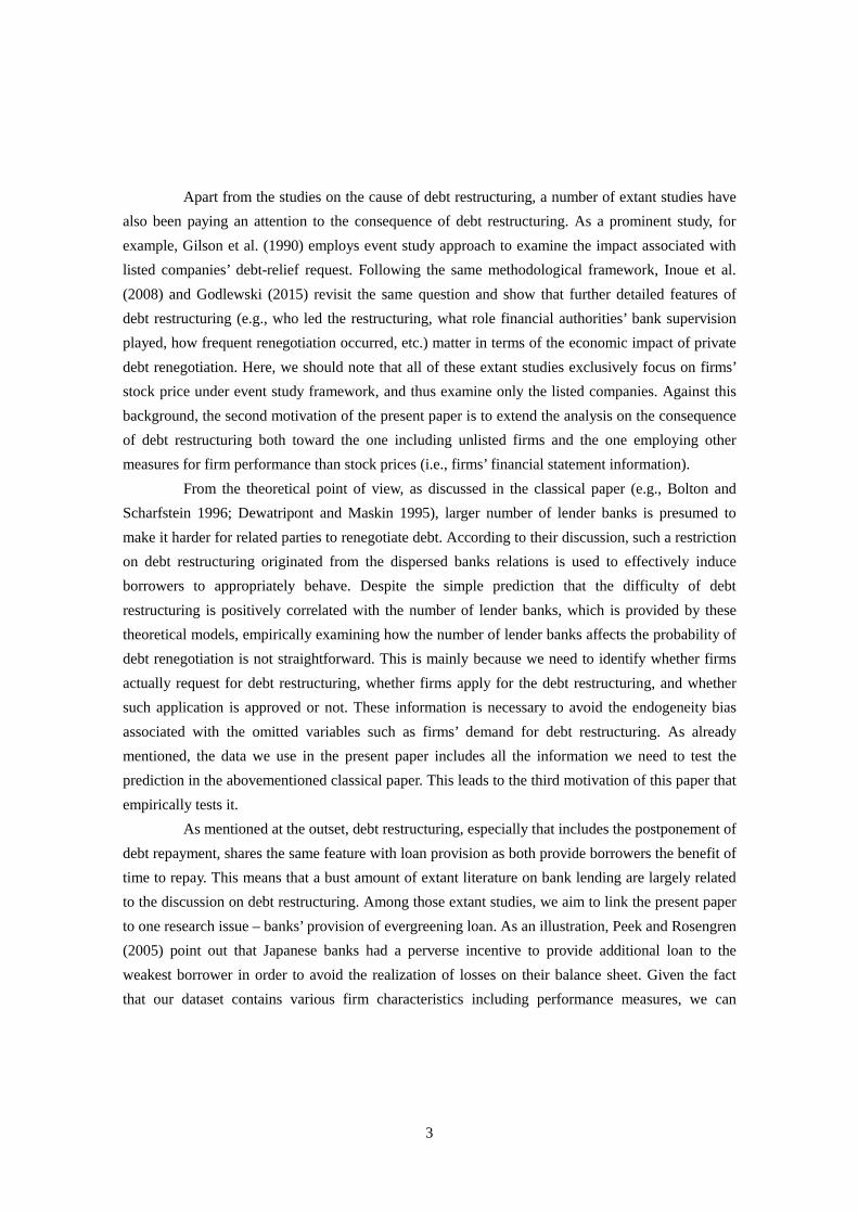
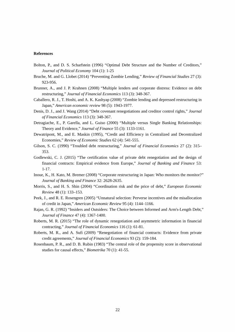
Among the questions of the survey, the question 19_2 accounts for the status of private debt restructuring. In this question, a categorical variable Choice takes one of the value from 1 to 5. Each number correspond to different status of debt restructuring as follows: 1 = firm requested debt restructuring and got approved, 2 = firm requested debt restructuring and got rejected, 3 = firm wanted to request but did not actually apply for as guessing the debt restructuring request would not be approved, 4 = firm wanted to request but did not as guessing debt restructuring request would negatively affect its bank relationship, and 5 = firm did not request as there was no need for debt restructuring. Figure 2 illustrates the structure of this question 19_2 and Table 1 tabulates the distribution of each response. We can see that more than 60% of the observation answered that they did not demand for debt restructuring. Among the rest of the observations, 1,548 firms requested debt restructuring and actually got approved. We should note that only 64 observations out of 6,002 responses account for “demanded but got rejected” while a certain number of firms (Choice = 3 and 4) gave up to request debt restructuring voluntarily although wanted to request. In the following analysis, we mainly identify the observation with demand as the ones with Choice = 1, 2, 3, or 4 (Demand: yes) while that without demand as the one with Choice = 5 (Demand: no), respectively. In

9

the case of using this identification, we use all the samples choosing 1, 2, 3, 4, or 5 for our analysis. We also employ alternative identification of the firms with the demand for debt renegotiation as the one with only Choice = 1 or 2. In the case of using this definition, we further employ two subcases using (i) Choice = 1, 2, 3, 4, and 5, or (2) 1, 2, and 5 as the data we use for our empirical analysis.

The survey contains wide variety of information accounting for firm performance, financial condition, lender banks’ characteristics, firms’ relationship with lender banks in multiple data points in addition to the status of debt restructuring mentioned above. In the next subsection, we detail how to use such information in our empirical analysis.

3.2. Empirical framework

The data explained in the previous section allows us to construct dummy variables (demand) taking value of one if the firm answers that it has demand for debt restructuring. Using the dummy variables accounting for demand, we estimate the determinants of the demand for debt restructuring. To be more precise, we assume that firm i demands for debt restructuring if its profits are larger when doing so than when not doing so. Let πi

* represent the difference between the profits of firm i when it demand for debt restructuring and its profits when not doing so. The difference is determined by the firm’s characteristics, including its financial condition, and the relationship between the firms and lender banks. Therefore, we parameterize πit

* as follows: 𝜋𝜋𝑖𝑖∗ = 𝛼𝛼 + 𝑭𝑭𝑭𝑭𝑭𝑭𝑭𝑭𝑖𝑖𝜷𝜷𝒅𝒅 + 𝑩𝑩𝑩𝑩𝑩𝑩𝑩𝑩𝑖𝑖𝜸𝜸𝒅𝒅 + 𝑭𝑭𝑹𝑹𝑹𝑹𝑩𝑩𝑹𝑹𝑭𝑭𝑹𝑹𝑩𝑩𝑖𝑖𝜹𝜹𝒅𝒅 + 𝜀𝜀𝑖𝑖 (1) where 𝑭𝑭𝑭𝑭𝑭𝑭𝑭𝑭𝑖𝑖, 𝑩𝑩𝑩𝑩𝑩𝑩𝑩𝑩𝑖𝑖, and 𝑭𝑭𝑹𝑹𝑹𝑹𝑩𝑩𝑹𝑹𝑭𝑭𝑹𝑹𝑩𝑩𝑖𝑖 denote the vectors of the characteristics of firm, main bank, and the relationship between them, respectively. The last term in the right hand-side of the equation εi captures unobserved firm characteristics and other unknown factors that may also affect differential profits. We assume that firm i demands for debt restructuring if differential profits πi

*>0. Under the assumption that εi is a normally distributed random error with zero mean and unit variance, the probability that firm i demands for debt restructuring can be written as follows: 𝑃𝑃𝑃𝑃𝑃𝑃𝑃𝑃(𝑑𝑑𝑑𝑑𝑑𝑑𝑑𝑑𝑑𝑑𝑑𝑑)𝑖𝑖 = 𝑃𝑃𝑃𝑃𝑃𝑃𝑃𝑃�𝛼𝛼 + 𝑭𝑭𝑭𝑭𝑭𝑭𝑭𝑭𝑖𝑖𝜷𝜷𝒅𝒅 + 𝑩𝑩𝑩𝑩𝑩𝑩𝑩𝑩𝑖𝑖𝜸𝜸𝒅𝒅 + 𝑭𝑭𝑹𝑹𝑹𝑹𝑩𝑩𝑹𝑹𝑭𝑭𝑹𝑹𝑩𝑩𝑖𝑖𝜹𝜹𝒅𝒅 + 𝜀𝜀𝑖𝑖 > 0� (2) We estimate equation (2) with a probit specification. The dependent variable Prob(demand)i denotes the change in demand status at the firm level and takes a value of one if a firm demands for debt restructuring.

Then, for the analysis of the approval of firms’ request for debt restructuring, we assume

10

that the main bank of firm i, which demands for debt restructuring, approves the request if its (i.e., banks’) profits are larger when doing so than when not doing so. Let πi

** represent the difference between the profits of the main bank for firm i when it approves and its profits when not doing so. Similarly to the assumption introduced for the analysis of the demand for debt restructuring, the difference is determined by the firm’s characteristics and the relationship between the firms and lender banks. Therefore, we parameterize πit

** and the probability that the main bank for firm i approves debt restructuring can be written as follows:

𝜋𝜋𝑖𝑖∗∗ = 𝛼𝛼 + 𝑭𝑭𝑭𝑭𝑭𝑭𝑭𝑭𝑖𝑖𝜷𝜷𝒂𝒂 + 𝑩𝑩𝑩𝑩𝑩𝑩𝑩𝑩𝑖𝑖𝜸𝜸𝒂𝒂 + 𝑭𝑭𝑹𝑹𝑹𝑹𝑩𝑩𝑹𝑹𝑭𝑭𝑹𝑹𝑩𝑩𝑖𝑖𝜹𝜹𝒂𝒂 + 𝜀𝜀𝑖𝑖 (3) 𝑃𝑃𝑃𝑃𝑃𝑃𝑃𝑃(𝑑𝑑𝑎𝑎𝑎𝑎𝑃𝑃𝑃𝑃𝑎𝑎𝑑𝑑)𝑖𝑖 = 𝑃𝑃𝑃𝑃𝑃𝑃𝑃𝑃(𝛼𝛼 + 𝑭𝑭𝑭𝑭𝑭𝑭𝑭𝑭𝑖𝑖𝜷𝜷𝒂𝒂 + 𝑩𝑩𝑩𝑩𝑩𝑩𝑩𝑩𝑖𝑖𝜸𝜸𝒂𝒂 + 𝑭𝑭𝑹𝑹𝑹𝑹𝑩𝑩𝑹𝑹𝑭𝑭𝑹𝑹𝑩𝑩𝑖𝑖𝜹𝜹𝒂𝒂 + 𝜀𝜀𝑖𝑖 > 0) (4) Using the observations of firms with demand for debt restructuring, we estimate equation (4) with a probit specification. The dependent variable Prob(approval)i denotes the change in the status of approval at the firm level and takes a value of one if a firms’ demand for debt restructuring was approved.

Among the questions in the survey, the question 29 and the question 39 ask the information related to how “temporary” the debt restructuring was. First, the question 29 asks the contents of debt restructuring. In this question 29, which allows multiple answers, a categorical variable Temp1 takes one of the value from 1 to 8. Each number corresponds to the content of debt restructuring as follows: 1 = the repayment of debt is postponed within one year, 2 the repayment of debt is postponed beyond one year, 3 = postponing principal repayment, 4 = reduction of interest payment, 5 = reduction of principal repayment, 6 = debt-equity swap, 7 = debt-debt swap, and 8 = others. Based on the information obtained from the answer to this question, we define a dummy variable TDR1, which takes the value of 1 if the answer to the question 29 (the contents of debt restructuring) does not contain (i) Temp1=4 or 5 (i.e., no reduction in principal or interests) or (ii) Temp1=2 (i.e., the postponement of repayment schedule is beyond one year), but contains (iii) Temp1=1 (i.e., the postponement of repayment is within one year).

Alternatively, a dummy variable TDR2 is defined to takes the value of one if the answer to the question 39 (reason for consecutive debt restructuring) is “the consecutive debt restructuring was predicted from onset” but does not contain any other reasons (i.e., business plan was no feasible, unexpected outside environment change, financial institution did not provided expected supports, lack of firms’ own effort). Following the same framework introduced above and using the sample with getting

11

request for debt restructuring approved, we let πi*** represent the difference between the profits of

the main bank for firm i in the case that it employs temporary debt restructuring scheme and in the case applying non-temporary debt restructuring scheme. Similarly to the abovementioned assumptions, the difference is determined by the firm’s characteristics, including its financial condition, the relationship between the firms and lender banks as well as bank characteristics. Therefore, we parameterize πit

*** and the probability that the main bank for firm i employs temporary debt restructuring scheme can be written as follows: 𝜋𝜋𝑖𝑖∗∗ = 𝛼𝛼 + 𝑭𝑭𝑭𝑭𝑭𝑭𝑭𝑭𝑖𝑖𝜷𝜷𝒂𝒂 + 𝑩𝑩𝑩𝑩𝑩𝑩𝑩𝑩𝑖𝑖𝜸𝜸𝒂𝒂 + 𝑭𝑭𝑹𝑹𝑹𝑹𝑩𝑩𝑹𝑹𝑭𝑭𝑹𝑹𝑩𝑩𝑖𝑖𝜹𝜹𝒂𝒂 + 𝜀𝜀𝑖𝑖 (5) Then, we estimate equation (6) with a probit specification. The dependent variable Prob(temp)i denotes the change in the content of restructuring, which is measured by whether it is temporary or not at the firm level and takes a value of one if the approved debt restructuring is temporary. 𝑃𝑃𝑃𝑃𝑃𝑃𝑃𝑃(𝑡𝑡𝑑𝑑𝑑𝑑𝑎𝑎)𝑖𝑖 = 𝑃𝑃𝑃𝑃𝑃𝑃𝑃𝑃(𝛼𝛼 + 𝑭𝑭𝑭𝑭𝑭𝑭𝑭𝑭𝑖𝑖𝜷𝜷𝒕𝒕𝒕𝒕𝒕𝒕𝒕𝒕 + 𝑩𝑩𝑩𝑩𝑩𝑩𝑩𝑩𝑖𝑖𝜸𝜸𝒕𝒕𝒕𝒕𝒕𝒕𝒕𝒕 + 𝑭𝑭𝑹𝑹𝑹𝑹𝑩𝑩𝑹𝑹𝑭𝑭𝑹𝑹𝑩𝑩𝑖𝑖𝜹𝜹𝒕𝒕𝒕𝒕𝒕𝒕𝒕𝒕 + 𝜀𝜀𝑖𝑖 > 0) (6)

Given these analyses for the determinants of the various dimensions of debt restructuring, we further implement the analysis on the consequence of temporary debt restructuring in terms of firm performance. In order to evaluate the causal impact running from the utilization of temporary debt restructuring on firm performance, first, we compute the propensity score defined in Rosenbaum and Rubin (1983), which is the conditional probability of assignment to a particular treatment (i.e., temporary debt restructuring in our case) given the pre-treatment characteristics:

𝑃𝑃(𝑥𝑥) ≡ 𝑃𝑃𝑃𝑃𝑃𝑃𝑃𝑃{𝑧𝑧 = 1|𝑥𝑥} = 𝐸𝐸{𝑧𝑧|𝑥𝑥} (7)

In this formulation, 𝑧𝑧 = {0,1} is the indicator of receiving the treatment and x is a vector

of observed pre-treatment characteristics. Rosenbaum and Rubin (1983) show that if the recipient of the treatment is randomly chosen within cells defined by x, it is also random within cells defined by the values of the single-index variable P(x). Therefore, for each treatment case j, if the propensity score 𝑃𝑃�𝑥𝑥𝑗𝑗� is known, the Average effect of Treatment on the Treated (ATT) can be estimated as follows:

𝛼𝛼�𝐴𝐴𝐴𝐴𝐴𝐴 = 𝐸𝐸�𝑦𝑦1𝑗𝑗 − 𝑦𝑦0𝑖𝑖|𝑧𝑧𝑗𝑗 = 1�

12

= 𝐸𝐸 �𝐸𝐸�𝑦𝑦1𝑗𝑗 − 𝑦𝑦0𝑗𝑗|𝑧𝑧𝑗𝑗 = 1,𝑎𝑎(𝑥𝑥𝑗𝑗)��

= 𝐸𝐸�𝐸𝐸�𝑦𝑦1𝑗𝑗|𝑧𝑧𝑗𝑗 = 1,𝑎𝑎(𝑥𝑥𝑗𝑗)� − 𝐸𝐸�𝑦𝑦0𝑗𝑗|𝑧𝑧𝑗𝑗 = 0,𝑎𝑎(𝑥𝑥𝑗𝑗)�|𝑧𝑧𝑗𝑗 = 1� (8)

In this formulation, 𝑦𝑦1 and 𝑦𝑦0 denote the potential outcomes in the two counterfactual

situations of treatment and no treatment, respectively. Therefore, according to the last line of equation (8), the ATT can be estimated as the average difference between the outcome of recipients and non-recipients of the treatment whose propensity scores 𝑃𝑃�𝑥𝑥𝑗𝑗� are identical. In the case of the presenting study, we specifically consider one type of treatment: temporary debt restructuring identified by TDR2. Therefore, we focus on the difference in ex-post performance between firms experiencing temporary debt restructuring and firms experiencing non-temporary debt restructuring.

Using the results of probit estimation in (6) at the first stage, we investigate important determinants of employing temporary debt restructuring and compute the propensity score (i.e., the probabilities of experiencing temporary debt restructuring) for each firm. Making use of this result, we conduct propensity score matching and compare the change in the performance of firms within the pairs of observations matched on the propensity score. In our matching process, firms are matched using one-to-one nearest neighbor matching without replacement.

In the second stage, we estimate a difference-in-differences (DID) estimator to evaluate the causal effect of temporary debt restructuring on firm performance variable. Note that, once we match treated and control firms, the only difference between firms with temporary and non-temporary debt restructuring is the content of debt restructuring. Therefore, we focus on the Average effect of Treatment on the Treated (ATT). The ATT can be estimated as equation (8) above, which, in the case of this study, is recovered from the estimation of the following equation using the dataset consist of the performance measures as of Decemper 2009 (1(𝑎𝑎𝑃𝑃𝑝𝑝𝑡𝑡𝑖𝑖) = 0) and the latest period (1(𝑎𝑎𝑃𝑃𝑝𝑝𝑡𝑡𝑖𝑖) = 1) for firms experiencing temporary debt restructuring and non-temporary debt restructuring.

𝑃𝑃𝑑𝑑𝑃𝑃𝑃𝑃𝑃𝑃𝑑𝑑𝑑𝑑𝑑𝑑𝑃𝑃𝑑𝑑𝑖𝑖 = 𝜃𝜃0 + 𝜃𝜃11(𝑡𝑡𝑑𝑑𝑑𝑑𝑎𝑎𝑖𝑖) + 𝜃𝜃21(𝑎𝑎𝑃𝑃𝑝𝑝𝑡𝑡𝑖𝑖) + 𝜃𝜃31(𝑡𝑡𝑑𝑑𝑑𝑑𝑎𝑎𝑖𝑖) × 1(𝑎𝑎𝑃𝑃𝑝𝑝𝑡𝑡𝑖𝑖) + 𝜀𝜀𝑖𝑖 (9)

where 1(𝑡𝑡𝑑𝑑𝑑𝑑𝑎𝑎𝑖𝑖) denotes the dummy variable taking the value of one if firm i experienced temporary debt restructuring. In this estimation, the coefficient associated with the interaction term (𝜃𝜃3) accounts for the causal (i.e., DID) effect of the temporary debt restructuring. In the present paper, we mainly use the credit score of firm i provided by TSR as a proxy for 𝑃𝑃𝑑𝑑𝑃𝑃𝑃𝑃𝑃𝑃𝑑𝑑𝑑𝑑𝑑𝑑𝑃𝑃𝑑𝑑𝑖𝑖. The score covers variety of firm characteristics in including creditworthiness, financial stability, growth opportunity, and subjective evaluation of firms provided by TSR. The score has 50 as its average and

13

raging from 0 to 100, the larger number of which corresponds to better evaluation. In order to see whether such DID effect depends on the timing of debt restructuring, we further introduce a dummy variable 1(𝑑𝑑𝑃𝑃𝑡𝑡𝑑𝑑𝑃𝑃𝑎𝑎𝑑𝑑𝑎𝑎𝑖𝑖) taking the value of one if the timing of debt restructuring for firm i is after march 2013 (i.e., after the termination of the SME financial act). 𝑃𝑃𝑑𝑑𝑃𝑃𝑃𝑃𝑃𝑃𝑑𝑑𝑑𝑑𝑑𝑑𝑃𝑃𝑑𝑑𝑖𝑖 = 𝜙𝜙0 + 𝜙𝜙11(𝑡𝑡𝑑𝑑𝑑𝑑𝑎𝑎𝑖𝑖) + 𝜙𝜙21(𝑎𝑎𝑃𝑃𝑝𝑝𝑡𝑡𝑖𝑖) + 𝜙𝜙31(𝑑𝑑𝑃𝑃𝑡𝑡𝑑𝑑𝑃𝑃𝑎𝑎𝑑𝑑𝑎𝑎𝑖𝑖) +𝜙𝜙41(𝑡𝑡𝑑𝑑𝑑𝑑𝑎𝑎𝑖𝑖) × 1(𝑎𝑎𝑃𝑃𝑝𝑝𝑡𝑡𝑖𝑖) + 𝜙𝜙51(𝑎𝑎𝑃𝑃𝑝𝑝𝑡𝑡𝑖𝑖) × 1(𝑑𝑑𝑃𝑃𝑡𝑡𝑑𝑑𝑃𝑃𝑎𝑎𝑑𝑑𝑎𝑎𝑖𝑖) + 𝜙𝜙61(𝑑𝑑𝑃𝑃𝑡𝑡𝑑𝑑𝑃𝑃𝑎𝑎𝑑𝑑𝑎𝑎𝑖𝑖) × 1(𝑡𝑡𝑑𝑑𝑑𝑑𝑎𝑎𝑖𝑖) +𝜙𝜙71(𝑡𝑡𝑑𝑑𝑑𝑑𝑎𝑎𝑖𝑖) × 1(𝑎𝑎𝑃𝑃𝑝𝑝𝑡𝑡𝑖𝑖) × 1(𝑑𝑑𝑃𝑃𝑡𝑡𝑑𝑑𝑃𝑃𝑎𝑎𝑑𝑑𝑎𝑎𝑖𝑖) + 𝜀𝜀𝑖𝑖 (10) In this estimation, the coefficient associated with the interaction term 1(𝑡𝑡𝑑𝑑𝑑𝑑𝑎𝑎𝑖𝑖) × 1(𝑎𝑎𝑃𝑃𝑝𝑝𝑡𝑡𝑖𝑖) (i.e., 𝜙𝜙4 ) accounts for the causal effect of the temporary debt restructuring in the case the debt restructuring was done before the termination of the SME financial act while the causal effect after the termination of the act is denoted by the sum (𝜙𝜙4 + 𝜙𝜙7). In the next section, we present the empirical results based on these frameworks and discuss the implication. 4. Empirical Analysis 4.1. Demand for debt restructuring

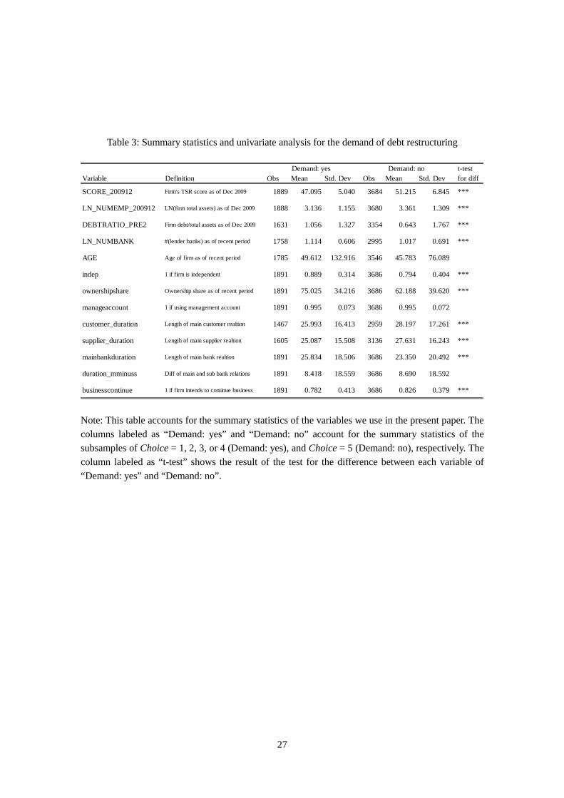
In this sub-section, we show the results based on the probit estimation on the determinants of the demand for debt restructuring. Before conducting detailed analyses, we first take a look at the results based on a univariate analysis. Table 3 accounts for the summary statistics of the variables we use to estimate the equation (2). The columns labeled as “Demand: yes” and “Demand: no” account for the summary statistics of the subsamples of Choice = 1, 2, 3, or 4 (i.e., Demand: yes), and Choice = 5 (i.e., Demand: no), respectively. The column labeled as “t-test” shows the result of the test for the difference between each variable of “Demand: yes” and “Demand: no”. The definition of each variable are in the table.

From Table 3, we can clearly see that it is more likely to demand debt restructuring if firms show lower credit worthiness (SCORE_200912), smaller size measured by the number of employees as of December 2009 (LN_NUMEMP_200912), larger debt burden as of December 2009 (DEBTRATIO_PRE2), larger number of lender banks (LN_NUMBANK), independent firm status (indep), higher ownership share (ownershipshare), shorter customer and supplier relationships (customer_duration and supplier_duration), and lower intention to continue its business (businesscontinue).

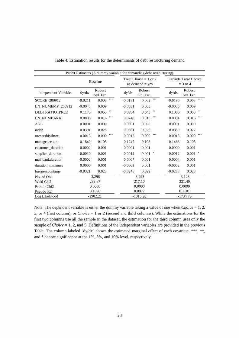
For these results, the estimated marginal effects obtained from obtained from probit estimation and summarized in Table 4 confirm that the negative impacts associated with

14

SCORE_200912 and the positive impact associated with DEBTRATIO_PRE2 on the probability of demanding for debt restructuring are significant in such a multivariate setup. These results imply that firms with lower creditworthiness and larger debt burden are more likely to find it more profitable to request debt restructuring. Second, it is also confirmed that firms with the larger number of lender banks are more likely to demand for debt restructuring. This result can be interpreted as an evidence that dispersed lender relationships makes it harder for firms to obtain additional loan so that the firms need to rely on debt restructuring once the firms face financial difficulty. Third, the positive correlation between the ownership share and the probability for demanding debt restructuring imply that owner of the business has some private benefit from continuing business.

4.2. Approval of debt restructuring So far, we have focused on firms’ demand for debt restructuring. As modeled in the

previous section, it crucially depends on banks’ motivation whether the request for debt restructuring is approved or not. First, Table 5 implements a univariate analysis, which accounts for the summary statistics of the variables for the observation with Choice is not equal to 5, i.e., the firms with demand for debt restructuring. The columns labeled as “Approval: yes” and “Approval: no” account for the summary statistics of the subsamples of Choice = 1 (i.e., Approval: yes) and Choice = 2, 3, or 4 (i.e., Approval: no), respectively. The column labeled as “t-test” shows the result of the test for the difference between each variable of “Approval: yes” and “Approval: no”.

Unlike the results in Table 3, we can find only a limited number of variables showing statistically significant difference between the two cases, i.e., “Approval: yes” and “Approval: no”. For example, only higher creditworthiness of firms (SCORE_200912), larger firms size (LN_NUMEMP_200912), longer main bank relationship (mainbankduraiton), and larger intention to continue business (businesscontinue) seem to contribute to higher probability of having debt restructuring approved.

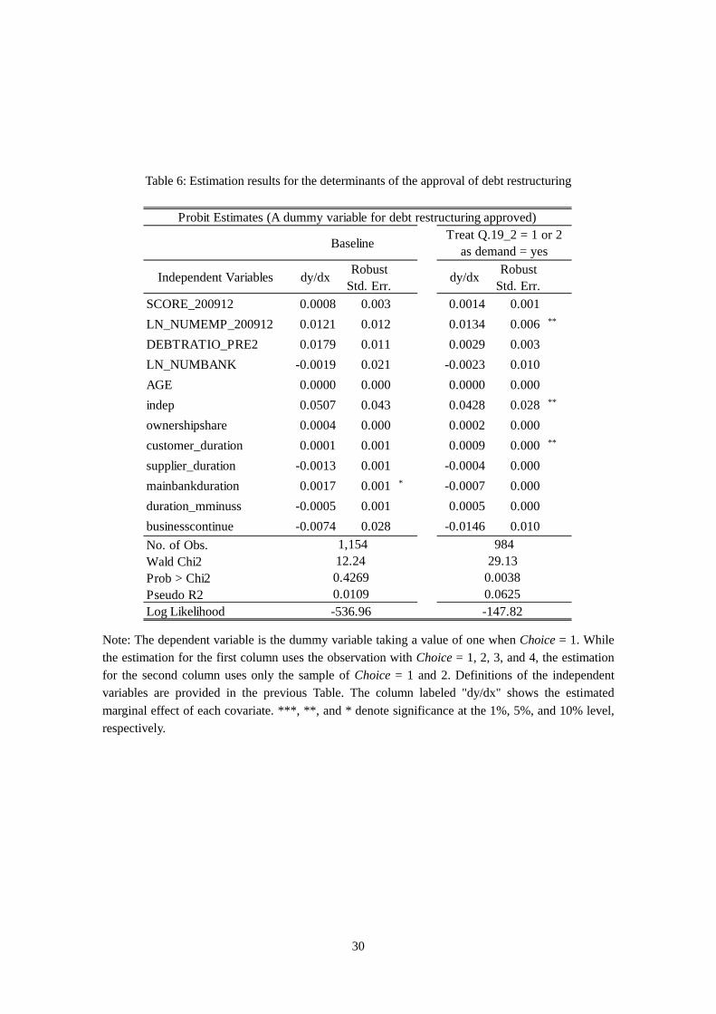
Although each of these results is intuitive, these are not necessarily supported by the results of the multivariate analysis summarized in Table 6. The dependent variable in Table 6 is the dummy variable taking a value of one when Choice = 1 (approved). While the estimation for the first column uses the observation with Choice = 1, 2, 3, and 4, the estimation for the second column uses only the sample of Choice = 1 and 2 to see the robustness of the result in the first column. From Table 6, we can see that the obtained results are not necessarily consistent between these two estimations and the explanatory power of the estimation in the first column is extremely low.

We presume that this result reflects the fact that rough information such as simply approval or not does not provide enough information for us to examine the mechanism governing the working

15

of debt restructuring. For example, the detailed contents of the restructuring (e.g., how long the repayment schedule is postponed or how much principal and interests are reduced) might be the necessary information to measure such the substance of debt restructuring. In the present paper, we assume that the mechanism behind the approval of debt restructuring depends on whether the debt restructuring is temporary or not. This could be identified by the variable TDR1 and TDR2. Whether the debt restructuring is temporary or not could be also identified by the information on if the pair of firm and bank are certain that they will renegotiate or not. In the next subsection, we explicitly examine this in more detail. 4.3. Employment of temporary debt restructuring

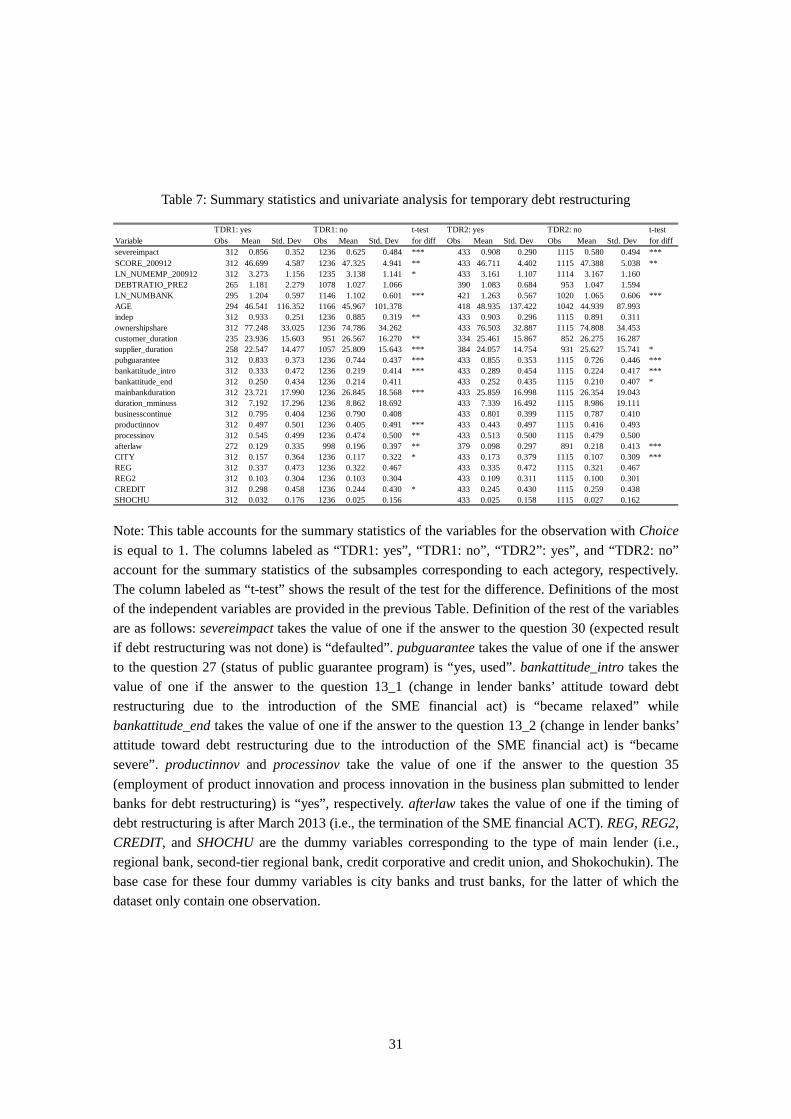
First, Table 7 implements a univariate analysis, which accounts for the summary statistics of the variables for the observation experiencing temporary debt restructuring measured by TDR1 (the first two columns) and TDR2 (the third and fourth columns). The columns labeled as “TDR1: yes” and “TDR1: no” account for the summary statistics of the subsamples of TDR1 = 1 and TDR1 = 0, respectively. The columns labeled as “TDR2: yes” and “TDR”: no” account for the summary statistics of the subsamples of TDR2 = 1 and TDR2 = 0, respectively. The column labeled as “t-test” shows the result of the test for the difference between each variable. We can see that, regardless of the identifier for temporary debt restructuring, it is more likely for temporary debt restructuring to be employed if firms show lower credit worthiness (SCORE_200912), larger number of lender banks (LN_NUMBANK), and shorter supplier relationship (supplier_duration). In addition to these results, we can also find that it is more likely for temporary debt restructuring to be employed if firms find it more important to get restructuring approved (severeimpact), rely on public guarantee (pubguarantee), lender banks react to the introduction of SME financial act in the way that the banks relaxed their attitude toward debt renegotiation (bankattitute_intro), and main bank is city bank (CITY). As one of the most important findings, we can also see that the temporary debt restructuring is less likely to be employed after the termination of the SME financial act (afterlaw).

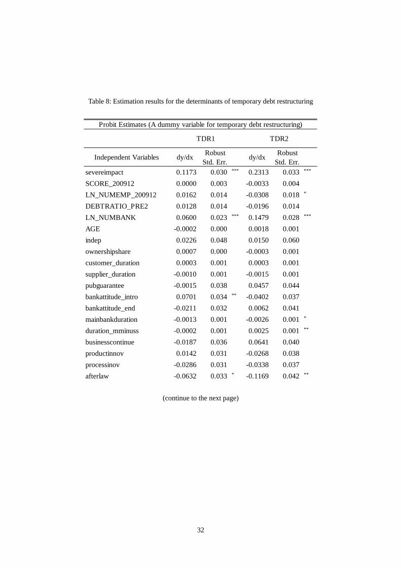
For these results, first, the two sets of the estimate results in Table 8 (i.e., based on TDR1 and TDR2) confirm that the positive impacts associated with LN_NUMBANK is significant even in such a multivariate setup. This result implies that the difficulty of coordination among multiple lenders for debt renegotiation results on the postponement of final decision of restructuring. This result is contrasting with that in Table 6 where LN_NUMBANK is not significant at all. While the number of banks does not seem to affect banks’ decision to approval, it matters for the more detailed contents of debt restructuring. This result suggests that it is necessary to use the information more

16

than the simple occurrence of debt restricting to study the mechanism behind debt restructuring. Second, it is also confirmed that the temporary debt restructuring is less likely to be employed after the termination of the SME financial act and in the case that firms find it more important to get the restructuring approved.

Table 9 repeats the same exercise by using multinomial logit specification accounting not only for whether debt restructuring is temporary or not but also for it is approved or not. This reflects our concern that exclusively focusing on the firms experiencing debt restructuring provides some selection bias to the results. In order to take into account such two selection process associated with (i) approved or not and (ii) temporary or not temporary, we set up a categorical variable taking avalue of 0 when debt restructuring is not approved, 1 when debt restructuring is approved andTDR1=0, and 2 when debt restructuring is approved and TDR1=1. We also construct the similarcategorical variable using TDR2 instead of TDR1. The dependent variable for the estimation of thefirst and second columns in Table 9 is using the variable based on TDR1 with using the variable=0as its base case. For the third and fourth column, the categorical variable based on TDR2 isemployed with using the variable=0 as its base case. In both cases, we use the sample of Choice = 1,2, 3, and 4 (i.e., firms with demand for debt restructuring). The results confirms the results in Table 8.Especially, compared to the case of not approved, the case of approved with temporary debtrestructuring (regardless of whether using TDR1 or TDR2) is more likely to be employed under thelarger number of lender banks. This result shows that the implication obtained from Table 8 does notseverely suffer from the selection bias associated with the sample selection.

4.4. Causal effect associated with temporary debt restructuring Using the estimate result in Table 8 (i.e., the case of TDR2) and following the equation (9),

we estimate how the employment of temporary debt restructuring affects firm performance. We also examine whether this effect (if any) is affected by the timing of debt restructuring.

The first column of Table 10 summarizes the estimate results based on (9). First, the negative coefficient associated with TDR implies that even in the analysis using the sample consisting of the firms matched by propensity-score, the firms experiencing temporary debt restructuring still shows ex-ante worse credit score than that experiencing non-temporary debt restructuring. Second, the negative coefficient associated with POST in the first column means that, over the sample periods, firms’ performance deteriorated on average. This result is consistent with the fact that the sample periods largely coincide with the periods right after the global financial crisis. Third, as the most important result, the negative coefficient associated with TDR*POST in the first column implies that the causal impact associated with temporary debt restructuring is negative. In

17

other words, firms experiencing temporary debt restructuring shows greater deterioration in its performance over the sample periods compared to the control group. We should note that the initial difference in the ex-ante credit score and the parallel change in the credit score for the treated (i.e., experiencing temporary debt restructuring) and the control are taken into account for in the estimation. This means that the employment of temporary debt restructuring statistically “causes” the deterioration of firm performance. Of course, even though we control for firm fixed-effect by using DID framework, there might be some unobservable time-variant factor, which we cannot observe but the lender banks can, affecting firm performance in different ways for the treated and the control. Thus, the interpretation of the result needs some caution. Notably, the result that the employment of temporary debt restructuring statistically causes the deterioration of firm performance might be the result of such an insider information held by lender banks.

How did the presence of the SME financial act affect this result? From the second column, which summarizes the estimate results based on the equation (10), we can see that the coefficient associated with TDR*POST*AFTERLAW is not statistically away from zero. Based on an additional test, furthermore, the null hypothesis that “the sum of the coefficients associated with TDR*POST and TDR*POST*AFTERLAW is equal to 0” is rejected in the significance at 10% level. This implies that regardless of whether debt restructuring was implemented before or after the termination of the SME financial act, the employment of temporary debt restructuring caused the deterioration of firm performance. We should note that this result might reflect the fact that Japanese FSA introduced three years of transitional period after the termination of the SME financial act on March 2013. In other words, over the all sample period, the act inducing banks to engage more debt restructuring was up to some extent effective. It would be an important future research question if the temporary debt restructuring is going to be associated with the abovementioned mal-effect even after this transition period.

While we confirm that the deterioration in firm performance caused by temporary debt restructuring is qualitatively unaffected by the presence or absence of the SME financial act, there is still a large variation in time to the end of the SME financial act. So far, we naively assume that the impact associated with temporary debt restructuring is not interacted with such time to the termination of the act, which might not be the case. Given this concern, we additionally estimate the following equation (11):

𝑃𝑃𝑑𝑑𝑃𝑃𝑃𝑃𝑃𝑃𝑑𝑑𝑑𝑑𝑑𝑑𝑃𝑃𝑑𝑑𝑖𝑖 = 𝜓𝜓0 + 𝜓𝜓11(𝑡𝑡𝑑𝑑𝑑𝑑𝑎𝑎𝑖𝑖) +𝜓𝜓31(𝑎𝑎𝑃𝑃𝑝𝑝𝑡𝑡𝑖𝑖) + 𝜓𝜓4𝑇𝑇𝑇𝑇𝑇𝑇𝐸𝐸𝑇𝑇𝑇𝑇𝐸𝐸𝑇𝑇𝑇𝑇𝑖𝑖 +𝜓𝜓51(𝑡𝑡𝑑𝑑𝑑𝑑𝑎𝑎𝑖𝑖) × 1(𝑎𝑎𝑃𝑃𝑝𝑝𝑡𝑡𝑖𝑖) + 𝜓𝜓61(𝑎𝑎𝑃𝑃𝑝𝑝𝑡𝑡𝑖𝑖) × 𝑇𝑇𝑇𝑇𝑇𝑇𝐸𝐸𝑇𝑇𝑇𝑇𝐸𝐸𝑇𝑇𝑇𝑇𝑖𝑖 +𝜓𝜓7𝑇𝑇𝑇𝑇𝑇𝑇𝐸𝐸𝑇𝑇𝑇𝑇𝐸𝐸𝑇𝑇𝑇𝑇𝑖𝑖 × 1(𝑡𝑡𝑑𝑑𝑑𝑑𝑎𝑎𝑖𝑖)+𝜓𝜓81(𝑡𝑡𝑑𝑑𝑑𝑑𝑎𝑎𝑖𝑖) × 1(𝑎𝑎𝑃𝑃𝑝𝑝𝑡𝑡𝑖𝑖) × 𝑇𝑇𝑇𝑇𝑇𝑇𝐸𝐸𝑇𝑇𝑇𝑇𝐸𝐸𝑇𝑇𝑇𝑇𝑖𝑖 + 𝜀𝜀𝑖𝑖 (11)

18

In the equation, 𝑇𝑇𝑇𝑇𝑇𝑇𝐸𝐸𝑇𝑇𝑇𝑇𝐸𝐸𝑇𝑇𝑇𝑇𝑖𝑖 stands for the number of months measured as the time to April 2013 from the data point of each temporary debt restructuring. It takes, for example, forty, in the case of the debt restructuring implemented on December 2009. We are interested in how the difference-in-difference effect denoted by 𝜓𝜓5 is interacted with 𝑇𝑇𝑇𝑇𝑇𝑇𝐸𝐸𝑇𝑇𝑇𝑇𝐸𝐸𝑇𝑇𝑇𝑇𝑖𝑖, which is captured by 𝜓𝜓8. The third column in Table 10 summarizes the estimate results. First, as we found in the previous estimation, there is a negative DID effect associated with temporary debt restructuring (i.e., 𝜓𝜓5=-2.1418). From the construction of our estimation, this number represents the DID effect for the case of temporary debt restructuring implemented on April 2013 where 𝑇𝑇𝑇𝑇𝑇𝑇𝐸𝐸𝑇𝑇𝑇𝑇𝐸𝐸𝑇𝑇𝑇𝑇𝑖𝑖 =0. Consistent with the previous result, we can see that even after the termination of the SME financial act, the employment of temporary debt restructuring statistically caused the deterioration of firm performance, which shows the robustness of our baseline result. Second, although it is only marginally statistically significant (i.e., 10%), the estimated coefficient associated with the triple interaction term 𝜓𝜓8 (0.0430) suggests that the abovementioned negative causal impact of temporary debt restructuring on firm performance was smaller for the case that temporary debt restructuring was implemented in the earlier period of our data. For example, given 𝑇𝑇𝑇𝑇𝑇𝑇𝐸𝐸𝑇𝑇𝑇𝑇𝐸𝐸𝑇𝑇𝑇𝑇𝑖𝑖 for the temporary debt restructuring implemented on December 2009 is forty, we can compute the DID effect for such case is -0.4218 (=-2.1418+0.0430*40), which is less than quarter of the abovementioned estimate (𝜓𝜓5=-2.1418), which corresponds to the DID effect for the case of temporary debt restructuring implemented on April 2013. This result means that the deterioration of firm performance caused by temporary debt restructuring became severer as the time passed by after the introduction of the SME financial act. One interpretation of this result could be that as such a distance becomes shorter, the negative causal impact associated with temporary debt restructuring becomes smaller since the length of periods for banks to hide the realization of loan losses becomes shorter. We should also note that this result in turn implies that the act was originally utilized for achieving its purpose, i.e., an urgent response to the global financial crisis.5 4.5. Other firm performance measures We have used so far the credit score of firm i provided by TSR as a proxy for

5 One limitation of the analysis based on the equation (11) is that we are assuming the effect of 𝑇𝑇𝑇𝑇𝑇𝑇𝐸𝐸𝑇𝑇𝑇𝑇𝐸𝐸𝑇𝑇𝑇𝑇𝑖𝑖 on the marginal effect associated with 1(𝑡𝑡𝑑𝑑𝑑𝑑𝑎𝑎𝑖𝑖) × 1(𝑎𝑎𝑃𝑃𝑝𝑝𝑡𝑡𝑖𝑖) is monotonic. This could not be the case when, for example, banks applied different policies toward debt restructuring over the sample period. An additional analysis taking into account the possibility of time-variant effect associated with 1(𝑡𝑡𝑑𝑑𝑑𝑑𝑎𝑎𝑖𝑖) × 1(𝑎𝑎𝑃𝑃𝑝𝑝𝑡𝑡𝑖𝑖) is one important future research issue.

19

𝑃𝑃𝑑𝑑𝑃𝑃𝑃𝑃𝑃𝑃𝑑𝑑𝑑𝑑𝑑𝑑𝑃𝑃𝑑𝑑𝑖𝑖 . While this score effectively summarizes firms characteristics spanning various dimensions in one number, it is difficult to see exactly what the change in this number means. The deterioration of the score could reflect, for example, the fact that firms own business condition got worse and/or some negative shocks were transmitted through their transaction partners (e.g., lender bank, supplier, and customers). To interpret our estimate results, it is important to see exactly what happened behind the negative DID effect associated with firms experiencing TDR. Toward this end, we implement the regression as in the equation (9) by using other measures for firm performance. Namely, we use firms’ subjective evaluation for the changes in “Business condition”, “Cash management”, and “Banks’ lending attitude” between December 2009 and October 2014 as well as the change in “Banks’ lending attitude” between the initial debt restructuring and October 2014. All the information is collected in the survey and recorded as the discrete numbers consisting of 1 (got better), 2 (slightly got better), 3 (unchanged), 4 (slightly got worse), and 5 (got worse). Since the dependent variable is not the ex-ante and ex-post levels but the change between these two data points, we run the following regression:

∆𝑃𝑃𝑑𝑑𝑃𝑃𝑃𝑃𝑃𝑃𝑑𝑑𝑑𝑑𝑑𝑑𝑃𝑃𝑑𝑑𝑖𝑖 = 𝜈𝜈0 + 𝜈𝜈11(𝑡𝑡𝑑𝑑𝑑𝑑𝑎𝑎𝑖𝑖) + 𝜀𝜀𝑖𝑖 (12)

In this formulation, the coefficient associated 1(𝑡𝑡𝑑𝑑𝑑𝑑𝑎𝑎𝑖𝑖) with represents the DID effect associated with TDR on the four performance measures.

Table 11 summarizes the estimate results based on the equation (12). First, we notice that the point estimate of the DID effect on firms’ business condition is negative and it is not statistically away from zero. This implies that firms experiencing TDR did not show worse performances than its control group as far as we focus on the firms’ own business condition. Second, on the other hand, once we employ the variables measuring firms financing environment, the point estimates are all positive (i.e., got worse). In particular, the DID effects on banks’ lending attitudes (i.e., third and fourth columns) show the positive impacts statistically away from zero. These results imply that the change in lending attitudes were the driver of the negative causal impact associated with TDR presented in the previous section. This could be the case, for example, when lender banks temporary restructured debt for the firms, for which the banks did not necessarily project the improvement in firm performance, mainly due to the introduction of the SME financial act, then tightened their lending attitudes later.

4.6. Interaction with lender bank characteristic One of the remained questions is why lender banks needed to commit such a temporary

20

treatment for their borrower firms. Since the SME financial act is valid only for a specific time period, banks cannot hide non-performing loan forever. One theoretical justification for such banks’ TDR is provided in Bruche and Llobet (2014) as distress banks have larger motivation for evergreening loan provision to their non-performing client firms. To check if their empirical implication is supported in our data set, we repeat the same regression in the first column of Table 10, the third column of Table 11, and the fourth column of Table 12 for the subsamples based on lender banks’ non-performing loan ratio (NPLratio). In this analysis, NPLratio is computed as the ratio of (i) the sum of the loan assets classified as bankrupt and the loan assets with delayed repayments to (ii) the total loan assets held by each lender bank as of the end of March 2009. We divide the sample above and below the sample median of NPLratio and test the prediction in Bruche and Llobet (2014). If firms borrowing from lender banks with weaker balance sheet conditions are more likely to experience TDR which end end up with the deterioration of firm performance, the prediction in Bruche and Llobet (2014) is supported. The second columns of the upper and lower panels of Table 12 show the consistent results with the above discussion. Namely, the DID effect on the changes in “Banks’ lending attitude” between December 2009 and October 2014 is statistically away from zero only for the lender banks with higher NPLratio. In the case that we change the firm performance measure to the changes in “Banks’ lending attitude” between the initial debt restructuring and October 2014, the DID effects are away from zero both in the case of higher and lower NPLratio, but the magnitude is larger for the lender banks with higher NPLratio. We should note that such a result is not necessarily obtained in the case using firms’ credit score for their performance measure (i.e., the first column in Table 12). This implies again that the DID effect on firm performance is mainly driven by banks’ side. In other words, lender banks (with weaker balance sheets) needed to commit TDR even though the SME financial act is valid only for a specific time period as the banks have large need to hide non-performing loan. 5. Conclusion

In this paper, we empirically analyze the cause and consequence of private debt restructuring out of court. Using a unique contract-level data accounting for Japanese bank loan, we find, first, that the demand of debt restructuring was systematically associated with firm characteristics and the relation-specific characteristics (esp., number of lender banks). Second, debt restructurings was more likely to take “temporary” form when the number of lender banks was larger and the SME financial act, which was introduced on December 2009 and terminated on March 2013, was effective. We also employ propensity score matching difference-in-difference estimation

21

to evaluate the causal impact of debt restructuring on firm performance, and find that the firms experiencing temporary debt restructuring exhibited the larger deterioration of its performance than the firms experiencing non-temporary debt restricting. Furthermore, such a pattern is more likely to be obtained when lender banks have weaker balance sheet conditions. The results in the present paper imply that temporary debt restructuring during our sample period was used as de facto evergreening, which ended up the deterioration of borrower creditworthiness. While debt restructuring could be theoretically used as an effective buffer for short-run shock, our finding shows that it is not necessarily the case in our dataset.

Our findings provide several policy implications. First, as we have already discussed, evergreening and zombie lending (e.g., Caballero et al. 2008) could be done under the form of temporary debt restructuring. Given this, for example, introduction of bank supervision explicitly taking into account the detailed contents of debt restructuring might be expected to avoid the temporary debt restructuring leading to the deterioration of firm performance. Second, our result shows that even after the termination of the SME financial act, the negative causal impact associated with temporary debt restructuring is observed. This suggests that the three years of transitional period after the termination of the SME financial act has been effectively inducing banks to keep their attitude toward debt restructuring. Third, our estimate results show that the effect of the SME financial act had been gradually digressed from its original purpose as time passed since its introduction. This suggests that sticking to a specific policy measure for unnecessarily long periods of time could generate unexpected side effect.

Finally, we would like to highlight potential avenues for future research. First, applying the same DID analysis framework to the employment of debt restructuring per se is one important future research issue. Although we have not done such an exercise since we have only limited number of observation we can use for the control (i.e., Choice = 2), it is still informative to select the control from the firms stating in the survey that they do not need debt restructuring. As far as the matching based on the propensity for firms to get debt restructuring approved is done precisely, the DID analysis associated with debt restructuring provide potentially useful implication. Second, another important extension would be to take the timing of debt restructuring more precisely. In the present study, we treated the timing of debt restructuring as simply either before or after the termination of the SME financial act, or the time to the termination of the act. In this regard, we can employ, for example, the dummy variable taking value of one for each data point where debt restructuring was implemented. We believe all of these potential extensions could provide further insights for a better understanding of private debt restructuring out of court, for which we have still had only limited understanding.

22

References Bolton, P., and D. S. Scharfstein (1996) “Optimal Debt Structure and the Number of Creditors,”

Journal of Political Economy 104 (1): 1-25 Bruche, M. and G. Llobet (2014) “Preventing Zombie Lending,” Review of Financial Studies 27 (3):

923-956. Brunner, A., and J. P. Krahnen (2008) “Multiple lenders and corporate distress: Evidence on debt

restructuring,” Journal of Financial Economics 113 (3): 348-367. Caballero, R. J., T. Hoshi, and A. K. Kashyap (2008) “Zombie lending and depressed restructuring in

Japan,” American economic review 98 (5): 1943-1977. Denis, D. J., and J. Wang (2014) “Debt covenant renegotiations and creditor control rights,” Journal

of Financial Economics 113 (3): 348-367. Detragiache, E., P. Garella, and L. Guiso (2000) “Multiple versus Single Banking Relationships:

Theory and Evidence,” Journal of Finance 55 (3): 1133-1161. Dewatripont, M., and E. Maskin (1995), “Credit and Efficiency in Centralized and Decentralized

Economies,” Review of Economic Studies 62 (4): 541-555. Gilson, S. C. (1990) “Troubled debt restructuring,” Journal of Financial Economics 27 (2): 315–

353. Godlewski, C. J. (2015) “The certification value of private debt renegotiation and the design of

financial contracts: Empirical evidence from Europe,” Journal of Banking and Finance 53: 1-17.

Inoue, K., H. Kato, M. Bremer (2008) “Corporate restructuring in Japan: Who monitors the monitor?” Journal of Banking and Finance 32: 2628-2635.

Morris, S., and H. S. Shin (2004) “Coordination risk and the price of debt,” European Economic Review 48 (1): 133–153.

Peek, J., and R. E. Rosengren (2005) “Unnatural selection: Perverse incentives and the misallocation of credit in Japan,” American Economic Review 95 (4): 1144–1166.

Rajan, G. R. (1992) “Insiders and Outsiders: The Choice between Informed and Arm's-Length Debt,” Journal of Finance 47 (4): 1367-1400.

Roberts, M. R. (2015) “The role of dynamic renegotiation and asymmetric information in financial contracting,” Journal of Financial Economics 116 (1): 61-81.

Roberts, M. R., and A. Sufi (2009) “Renegotiation of financial contracts: Evidence from private credit agreements,” Journal of Financial Economics 93 (2): 159-184.

Rosenbaum, P. R., and D. B. Rubin (1983) “The central role of the propensity score in observational studies for causal effects,” Biometrika 70 (1): 41-55.

23

Tables and Figure

Figure 1: Example of temporary debt restructuring

Note: The horizontal axis in the figures accounts for the time horizon. Each box corresponds the amounts of principal and interest payments at each point. The upper and lower panels illustrate the debt repayment schedule before and after the temporary debt restructuring where only the principal circled by dashed line is postponed without any reduction in principal or interests.

Time

Prin

cipa

l

Prin

cipa

l

Prin

cipa

l

Prin

cipa

l

Time

Prin

cipa

l

Prin

cipa

l

Prin

cipa

l

Prin

cipa

l

Prin

cipa

l

Interest Interest Interest Interest Interest

InterestInterest

Interest

Interest

Interest

Prin

cipa

l

Interest

Interest Interest

24

Figure 2: Question for debt restructuring

Note: The figure illustrates the contents of the question 19_2.

Debt restructured

All observations

Without demand for debt restructuring

2. Applied but rejected1. Applied and approved3. & 4. Wanted but not applied (self-constrained)

5. No need to apply

Notdebt restructured

With demand for debt restructuring

25

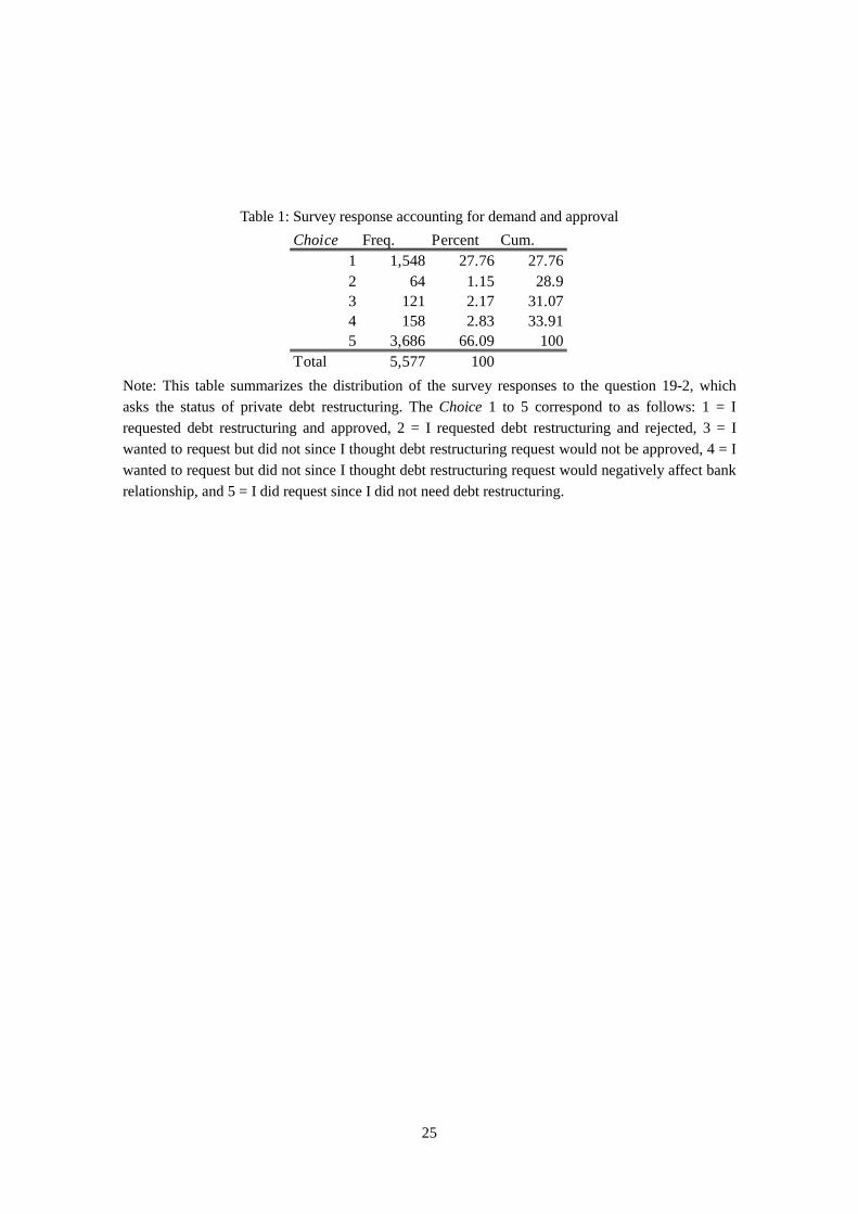
Table 1: Survey response accounting for demand and approval

Note: This table summarizes the distribution of the survey responses to the question 19-2, which asks the status of private debt restructuring. The Choice 1 to 5 correspond to as follows: 1 = I requested debt restructuring and approved, 2 = I requested debt restructuring and rejected, 3 = I wanted to request but did not since I thought debt restructuring request would not be approved, 4 = I wanted to request but did not since I thought debt restructuring request would negatively affect bank relationship, and 5 = I did request since I did not need debt restructuring.

Choice Freq. Percent Cum.1 1,548 27.76 27.762 64 1.15 28.93 121 2.17 31.074 158 2.83 33.915 3,686 66.09 100

Total 5,577 100

26

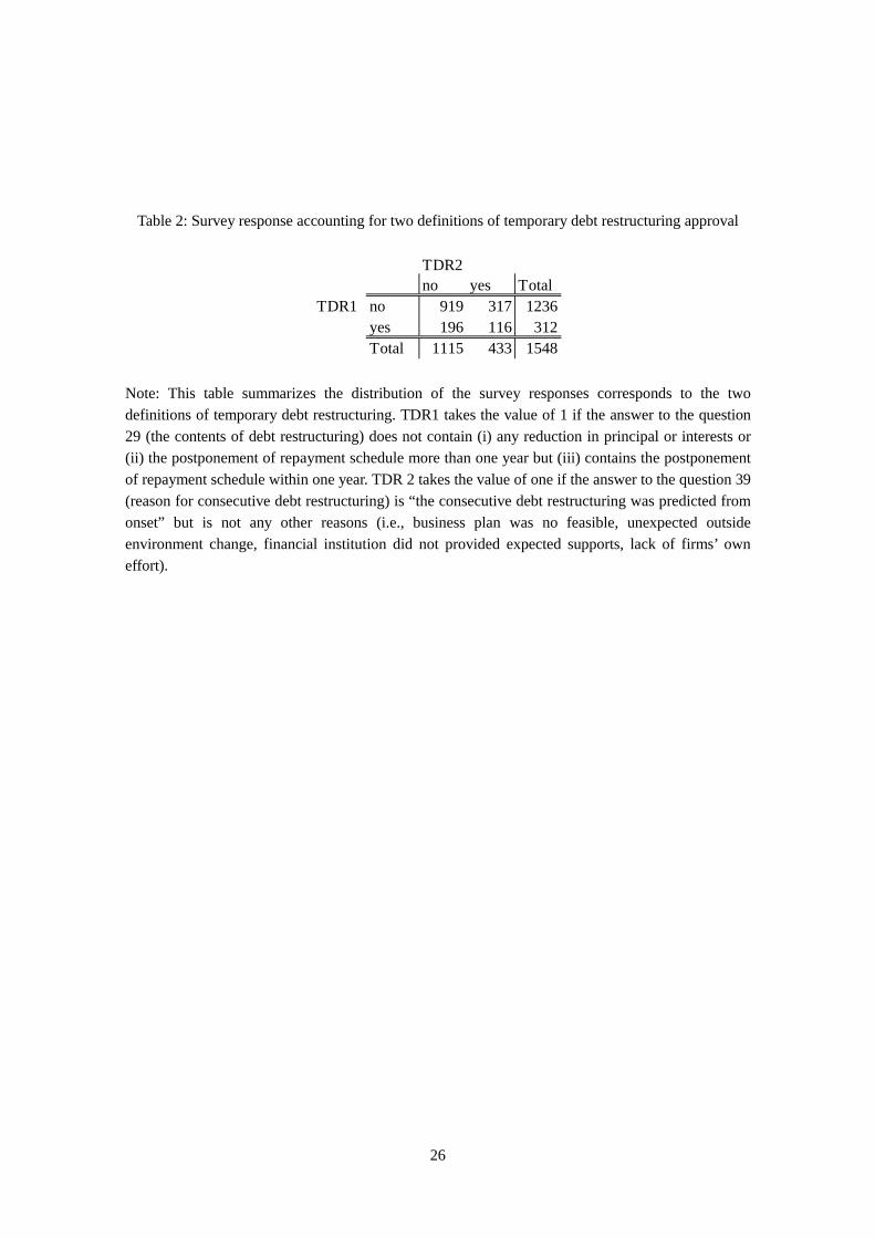
Table 2: Survey response accounting for two definitions of temporary debt restructuring approval

Note: This table summarizes the distribution of the survey responses corresponds to the two definitions of temporary debt restructuring. TDR1 takes the value of 1 if the answer to the question 29 (the contents of debt restructuring) does not contain (i) any reduction in principal or interests or (ii) the postponement of repayment schedule more than one year but (iii) contains the postponement of repayment schedule within one year. TDR 2 takes the value of one if the answer to the question 39 (reason for consecutive debt restructuring) is “the consecutive debt restructuring was predicted from onset” but is not any other reasons (i.e., business plan was no feasible, unexpected outside environment change, financial institution did not provided expected supports, lack of firms’ own effort).

TDR2no yes Total

TDR1 no 919 317 1236yes 196 116 312Total 1115 433 1548

27

Table 3: Summary statistics and univariate analysis for the demand of debt restructuring

Note: This table accounts for the summary statistics of the variables we use in the present paper. The columns labeled as “Demand: yes” and “Demand: no” account for the summary statistics of the subsamples of Choice = 1, 2, 3, or 4 (Demand: yes), and Choice = 5 (Demand: no), respectively. The column labeled as “t-test” shows the result of the test for the difference between each variable of “Demand: yes” and “Demand: no”.

t-testVariable Definition Obs Mean Std. Dev Obs Mean Std. Dev for diff

SCORE_200912 Firm's TSR score as of Dec 2009 1889 47.095 5.040 3684 51.215 6.845 ***

LN_NUMEMP_200912 LN(firm total assets) as of Dec 2009 1888 3.136 1.155 3680 3.361 1.309 ***

DEBTRATIO_PRE2 Firm debt/total assets as of Dec 2009 1631 1.056 1.327 3354 0.643 1.767 ***

LN_NUMBANK #(lender banks) as of recent period 1758 1.114 0.606 2995 1.017 0.691 ***

AGE Age of firm as of recent period 1785 49.612 132.916 3546 45.783 76.089

indep 1 if firm is independent 1891 0.889 0.314 3686 0.794 0.404 ***

ownershipshare Ownership share as of recent period 1891 75.025 34.216 3686 62.188 39.620 ***

manageaccount 1 if using management account 1891 0.995 0.073 3686 0.995 0.072

customer_duration Length of main customer realtion 1467 25.993 16.413 2959 28.197 17.261 ***

supplier_duration Length of main supplier realtion 1605 25.087 15.508 3136 27.631 16.243 ***

mainbankduration Length of main bank realtion 1891 25.834 18.506 3686 23.350 20.492 ***

duration_mminuss Diff of main and sub bank relations 1891 8.418 18.559 3686 8.690 18.592

businesscontinue 1 if firm intends to continue business 1891 0.782 0.413 3686 0.826 0.379 ***

Demand: yes Demand: no

28

Table 4: Estimation results for the determinants of debt restructuring demand

Note: The dependent variable is either the dummy variable taking a value of one when Choice = 1, 2, 3, or 4 (first column), or Choice = 1 or 2 (second and third columns). While the estimations for the first two columns use all the sample in the dataset, the estimation for the third column uses only the sample of Choice = 1, 2, and 5. Definitions of the independent variables are provided in the previous Table. The column labeled "dy/dx" shows the estimated marginal effect of each covariate. ***, **, and * denote significance at the 1%, 5%, and 10% level, respectively.

Independent Variables dy/dx RobustStd. Err.

dy/dx RobustStd. Err.

dy/dx RobustStd. Err.

SCORE_200912 -0.0211 0.003 *** -0.0181 0.002 *** -0.0196 0.003 ***

LN_NUMEMP_200912 -0.0043 0.009 -0.0031 0.008 -0.0035 0.009DEBTRATIO_PRE2 0.1173 0.053 ** 0.0994 0.045 ** 0.1086 0.050 **

LN_NUMBANK 0.0886 0.016 *** 0.0740 0.015 *** 0.0834 0.016 ***

AGE 0.0001 0.000 0.0001 0.000 0.0001 0.000indep 0.0391 0.028 0.0361 0.026 0.0380 0.027ownershipshare 0.0013 0.000 *** 0.0012 0.000 *** 0.0013 0.000 ***

manageaccount 0.1840 0.105 0.1247 0.108 0.1468 0.105customer_duration 0.0002 0.001 -0.0001 0.001 0.0000 0.001supplier_duration -0.0010 0.001 -0.0012 0.001 * -0.0012 0.001 *

mainbankduration -0.0002 0.001 0.0007 0.001 0.0004 0.001duration_mminuss 0.0000 0.001 -0.0003 0.001 -0.0002 0.001businesscontinue -0.0321 0.023 -0.0245 0.022 -0.0288 0.023No. of Obs.Wald Chi2Prob > Chi2Pseudo R2Log Likelihood

Probit Estimates (A dummy variable for demanding debt restructuring)Treat Choice = 1 or 2

as demand = yesExclude Treat Choice

= 3 or 4Baseline

3,128221.400.00000.1101

-1734.73

233.67

0.1096-1902.21

0.0000

3,298 3,298

0.0977-1815.28

217.100.0000

29

Table 5: Summary statistics and univariate analysis for the approval of debt restructuring

Note: This table accounts for the summary statistics of the variables for the observation with Choice is not equal to 5. The columns labeled as “Approval: yes” and “Approval: no” account for the summary statistics of the subsamples of Choice = 1 (Approval: yes) and Choice = 2, 3, or 4 (Approval: no), respectively. The column labeled as “t-test” shows the result of the test for the difference between each variable of “Approval: yes” and “Approval: no”.

t-testVariable Definition Obs Mean Std. Dev Obs Mean Std. Dev for diff

SCORE_200912 Firm's TSR score as of Dec 2009 1548 47.199 4.877 341 46.625 5.707 *

LN_NUMEMP_200912 LN(firm total assets) as of Dec 2009 1547 3.165 1.145 341 3.001 1.193 **

DEBTRATIO_PRE2 Firm debt/total assets as of Dec 2009 1343 1.057 1.392 288 1.052 0.968

LN_NUMBANK #(lender banks) as of recent period 1441 1.123 0.601 317 1.071 0.625

AGE Age of firm as of recent period 1460 46.083 104.524 325 65.465 218.562

indep 1 if firm is independent 1548 0.895 0.307 343 0.863 0.344

ownershipshare Ownership share as of recent period 1548 75.282 34.020 343 73.862 35.115

customer_duration Length of main customer realtion 1186 26.046 16.167 281 25.772 17.438

supplier_duration Length of main supplier realtion 1315 25.169 15.470 290 24.717 15.701

mainbankduration Length of main bank realtion 1548 26.216 18.490 343 24.114 18.509 *

duration_mminuss Diff of main and sub bank relations 1548 8.526 18.426 343 7.933 19.167

businesscontinue 1 if firm intends to continue business 1548 0.791 0.407 343 0.743 0.437 *

Approval: yes Approval: no

30

Table 6: Estimation results for the determinants of the approval of debt restructuring

Note: The dependent variable is the dummy variable taking a value of one when Choice = 1. While the estimation for the first column uses the observation with Choice = 1, 2, 3, and 4, the estimation for the second column uses only the sample of Choice = 1 and 2. Definitions of the independent variables are provided in the previous Table. The column labeled "dy/dx" shows the estimated marginal effect of each covariate. ***, **, and * denote significance at the 1%, 5%, and 10% level, respectively.

Independent Variables dy/dx RobustStd. Err.

dy/dx RobustStd. Err.

SCORE_200912 0.0008 0.003 0.0014 0.001LN_NUMEMP_200912 0.0121 0.012 0.0134 0.006 **

DEBTRATIO_PRE2 0.0179 0.011 0.0029 0.003LN_NUMBANK -0.0019 0.021 -0.0023 0.010AGE 0.0000 0.000 0.0000 0.000indep 0.0507 0.043 0.0428 0.028 **

ownershipshare 0.0004 0.000 0.0002 0.000customer_duration 0.0001 0.001 0.0009 0.000 **

supplier_duration -0.0013 0.001 -0.0004 0.000mainbankduration 0.0017 0.001 * -0.0007 0.000duration_mminuss -0.0005 0.001 0.0005 0.000businesscontinue -0.0074 0.028 -0.0146 0.010No. of Obs.Wald Chi2Prob > Chi2Pseudo R2Log Likelihood -536.96 -147.82

0.4269 0.00380.0109 0.0625

1,154 98412.24 29.13

Probit Estimates (A dummy variable for debt restructuring approved)Treat Q.19_2 = 1 or 2

as demand = yesBaseline

31

Table 7: Summary statistics and univariate analysis for temporary debt restructuring

Note: This table accounts for the summary statistics of the variables for the observation with Choice is equal to 1. The columns labeled as “TDR1: yes”, “TDR1: no”, “TDR2”: yes”, and “TDR2: no” account for the summary statistics of the subsamples corresponding to each actegory, respectively. The column labeled as “t-test” shows the result of the test for the difference. Definitions of the most of the independent variables are provided in the previous Table. Definition of the rest of the variables are as follows: severeimpact takes the value of one if the answer to the question 30 (expected result if debt restructuring was not done) is “defaulted”. pubguarantee takes the value of one if the answer to the question 27 (status of public guarantee program) is “yes, used”. bankattitude_intro takes the value of one if the answer to the question 13_1 (change in lender banks’ attitude toward debt restructuring due to the introduction of the SME financial act) is “became relaxed” while bankattitude_end takes the value of one if the answer to the question 13_2 (change in lender banks’ attitude toward debt restructuring due to the introduction of the SME financial act) is “became severe”. productinnov and processinov take the value of one if the answer to the question 35 (employment of product innovation and process innovation in the business plan submitted to lender banks for debt restructuring) is “yes”, respectively. afterlaw takes the value of one if the timing of debt restructuring is after March 2013 (i.e., the termination of the SME financial ACT). REG, REG2, CREDIT, and SHOCHU are the dummy variables corresponding to the type of main lender (i.e., regional bank, second-tier regional bank, credit corporative and credit union, and Shokochukin). The base case for these four dummy variables is city banks and trust banks, for the latter of which the dataset only contain one observation.

TDR1: yes TDR1: no t-test TDR2: yes TDR2: no t-testVariable Obs Mean Std. Dev Obs Mean Std. Dev for diff Obs Mean Std. Dev Obs Mean Std. Dev for diffsevereimpact 312 0.856 0.352 1236 0.625 0.484 *** 433 0.908 0.290 1115 0.580 0.494 ***SCORE_200912 312 46.699 4.587 1236 47.325 4.941 ** 433 46.711 4.402 1115 47.388 5.038 **LN_NUMEMP_200912 312 3.273 1.156 1235 3.138 1.141 * 433 3.161 1.107 1114 3.167 1.160DEBTRATIO_PRE2 265 1.181 2.279 1078 1.027 1.066 390 1.083 0.684 953 1.047 1.594LN_NUMBANK 295 1.204 0.597 1146 1.102 0.601 *** 421 1.263 0.567 1020 1.065 0.606 ***AGE 294 46.541 116.352 1166 45.967 101.378 418 48.935 137.422 1042 44.939 87.993indep 312 0.933 0.251 1236 0.885 0.319 ** 433 0.903 0.296 1115 0.891 0.311ownershipshare 312 77.248 33.025 1236 74.786 34.262 433 76.503 32.887 1115 74.808 34.453customer_duration 235 23.936 15.603 951 26.567 16.270 ** 334 25.461 15.867 852 26.275 16.287supplier_duration 258 22.547 14.477 1057 25.809 15.643 *** 384 24.057 14.754 931 25.627 15.741 *pubguarantee 312 0.833 0.373 1236 0.744 0.437 *** 433 0.855 0.353 1115 0.726 0.446 ***bankattitude_intro 312 0.333 0.472 1236 0.219 0.414 *** 433 0.289 0.454 1115 0.224 0.417 ***bankattitude_end 312 0.250 0.434 1236 0.214 0.411 433 0.252 0.435 1115 0.210 0.407 *mainbankduration 312 23.721 17.990 1236 26.845 18.568 *** 433 25.859 16.998 1115 26.354 19.043duration_mminuss 312 7.192 17.296 1236 8.862 18.692 433 7.339 16.492 1115 8.986 19.111businesscontinue 312 0.795 0.404 1236 0.790 0.408 433 0.801 0.399 1115 0.787 0.410productinnov 312 0.497 0.501 1236 0.405 0.491 *** 433 0.443 0.497 1115 0.416 0.493processinov 312 0.545 0.499 1236 0.474 0.500 ** 433 0.513 0.500 1115 0.479 0.500afterlaw 272 0.129 0.335 998 0.196 0.397 ** 379 0.098 0.297 891 0.218 0.413 ***CITY 312 0.157 0.364 1236 0.117 0.322 * 433 0.173 0.379 1115 0.107 0.309 ***REG 312 0.337 0.473 1236 0.322 0.467 433 0.335 0.472 1115 0.321 0.467REG2 312 0.103 0.304 1236 0.103 0.304 433 0.109 0.311 1115 0.100 0.301CREDIT 312 0.298 0.458 1236 0.244 0.430 * 433 0.245 0.430 1115 0.259 0.438SHOCHU 312 0.032 0.176 1236 0.025 0.156 433 0.025 0.158 1115 0.027 0.162

32

Table 8: Estimation results for the determinants of temporary debt restructuring

(continue to the next page)

Independent Variables dy/dx RobustStd. Err.

dy/dx RobustStd. Err.

severeimpact 0.1173 0.030 *** 0.2313 0.033 ***

SCORE_200912 0.0000 0.003 -0.0033 0.004LN_NUMEMP_200912 0.0162 0.014 -0.0308 0.018 *

DEBTRATIO_PRE2 0.0128 0.014 -0.0196 0.014LN_NUMBANK 0.0600 0.023 *** 0.1479 0.028 ***

AGE -0.0002 0.000 0.0018 0.001indep 0.0226 0.048 0.0150 0.060ownershipshare 0.0007 0.000 -0.0003 0.001customer_duration 0.0003 0.001 0.0003 0.001supplier_duration -0.0010 0.001 -0.0015 0.001pubguarantee -0.0015 0.038 0.0457 0.044bankattitude_intro 0.0701 0.034 ** -0.0402 0.037bankattitude_end -0.0211 0.032 0.0062 0.041mainbankduration -0.0013 0.001 -0.0026 0.001 *

duration_mminuss -0.0002 0.001 0.0025 0.001 **

businesscontinue -0.0187 0.036 0.0641 0.040productinnov 0.0142 0.031 -0.0268 0.038processinov -0.0286 0.031 -0.0338 0.037afterlaw -0.0632 0.033 * -0.1169 0.042 **

TDR1

Probit Estimates (A dummy variable for temporary debt restructuring)

TDR2

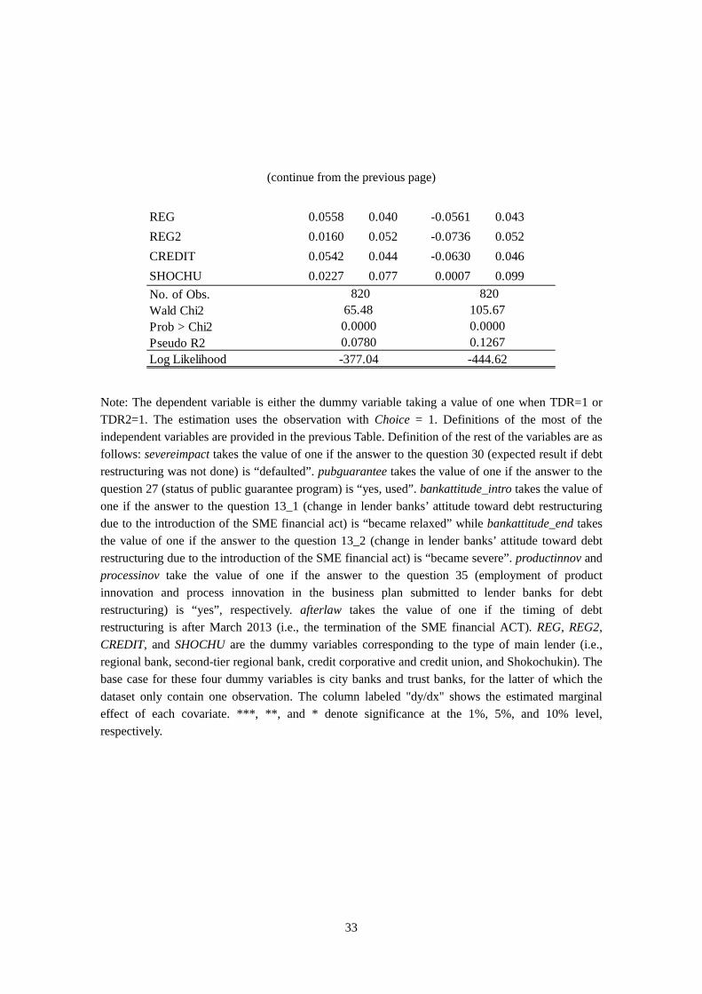
33

(continue from the previous page)

Note: The dependent variable is either the dummy variable taking a value of one when TDR=1 or TDR2=1. The estimation uses the observation with Choice = 1. Definitions of the most of the independent variables are provided in the previous Table. Definition of the rest of the variables are as follows: severeimpact takes the value of one if the answer to the question 30 (expected result if debt restructuring was not done) is “defaulted”. pubguarantee takes the value of one if the answer to the question 27 (status of public guarantee program) is “yes, used”. bankattitude_intro takes the value of one if the answer to the question 13_1 (change in lender banks’ attitude toward debt restructuring due to the introduction of the SME financial act) is “became relaxed” while bankattitude_end takes the value of one if the answer to the question 13_2 (change in lender banks’ attitude toward debt restructuring due to the introduction of the SME financial act) is “became severe”. productinnov and processinov take the value of one if the answer to the question 35 (employment of product innovation and process innovation in the business plan submitted to lender banks for debt restructuring) is “yes”, respectively. afterlaw takes the value of one if the timing of debt restructuring is after March 2013 (i.e., the termination of the SME financial ACT). REG, REG2, CREDIT, and SHOCHU are the dummy variables corresponding to the type of main lender (i.e., regional bank, second-tier regional bank, credit corporative and credit union, and Shokochukin). The base case for these four dummy variables is city banks and trust banks, for the latter of which the dataset only contain one observation. The column labeled "dy/dx" shows the estimated marginal effect of each covariate. ***, **, and * denote significance at the 1%, 5%, and 10% level, respectively.

REG 0.0558 0.040 -0.0561 0.043REG2 0.0160 0.052 -0.0736 0.052CREDIT 0.0542 0.044 -0.0630 0.046SHOCHU 0.0227 0.077 0.0007 0.099No. of Obs.Wald Chi2Prob > Chi2Pseudo R2Log Likelihood

820105.670.00000.1267-444.62

82065.480.00000.0780-377.04

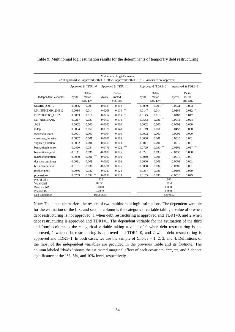
34

Table 9: Multinomial logit estimation results for the determinants of temporary debt restructuring

Note: The table summarizes the results of two multinomial logit estimations. The dependent variable for the estimation of the first and second column is the categorical variable taking a value of 0 when debt restructuring is not approved, 1 when debt restructuring is approved and TDR1=0, and 2 when debt restructuring is approved and TDR1=1. The dependent variable for the estimation of the third and fourth column is the categorical variable taking a value of 0 when debt restructuring is not approved, 1 when debt restructuring is approved and TDR1=0, and 2 when debt restructuring is approved and TDR1=1. In both cases, we use the sample of Choice = 1, 2, 3, and 4. Definitions of the most of the independent variables are provided in the previous Table and its footnote. The column labeled "dy/dx" shows the estimated marginal effect of each covariate. ***, **, and * denote significance at the 1%, 5%, and 10% level, respectively.

Independent Variables dy/dxDelta-metod

Std. Err.dy/dx

Delta-metod

Std. Err.dy/dx

Delta-metod

Std. Err.dy/dx

Delta-metod

Std. Err.

SCORE_200912 -0.0006 0.003 -0.0039 0.002 ** 0.0059 0.003 ** -0.0044 0.003LN_NUMEMP_200912 -0.0084 0.014 0.0208 0.010 ** -0.0147 0.014 0.0261 0.012 **

DEBTRATIO_PRE2 0.0063 0.016 0.0214 0.011 ** -0.0145 0.013 0.0187 0.012LN_NUMBANK -0.0217 0.027 0.0453 0.019 ** -0.0543 0.026 ** 0.0542 0.024 **

AGE 0.0002 0.000 -0.0002 0.000 0.0002 0.000 -0.0002 0.000indep 0.0004 0.050 0.0370 0.041 -0.0119 0.051 0.0453 0.050ownershipshare -0.0001 0.000 0.0004 0.000 -0.0002 0.000 0.0005 0.000customer_duration 0.0002 0.001 0.0007 0.001 0.0000 0.001 0.0010 0.001supplier_duration -0.0002 0.001 -0.0013 0.001 0.0011 0.001 -0.0015 0.001bankattitude_intro -0.0460 0.034 0.0771 0.022 *** -0.0729 0.030 ** 0.0866 0.027 ***

bankattitude_end -0.0111 0.036 -0.0180 0.025 -0.0291 0.033 -0.0238 0.030mainbankduration 0.0030 0.001 *** -0.0007 0.001 0.0010 0.001 -0.0015 0.001duration_mminuss -0.0011 0.001 0.0002 0.001 0.0000 0.001 0.0003 0.001businesscontinue -0.0161 0.036 -0.0201 0.026 -0.0060 0.034 -0.0207 0.031productinnov 0.0046 0.032 0.0227 0.024 -0.0237 0.031 0.0193 0.029processinov 0.0783 0.032 ** 0.0132 0.024 0.0155 0.030 -0.0010 0.029No. of Obs.Wald Chi2Prob > Chi2Pseudo R2Log Likelihood

Multinomial Logit Estimates(Not approved vs. Approved with TDR=0 vs. Approved with TDR=1 (Basecase = not approved)

Approved & TDR1=1 Approved & TDR2=1Approved & TDR2=0Approved & TDR1=0

1,22889.360.00000.0392

-1083.3634

98689.4

0.00000.0609

-589.0959

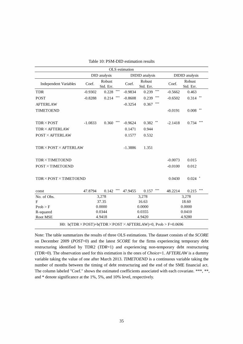
35

Table 10: PSM-DID estimation results

Note: The table summarizes the results of three OLS estimations. The dataset consists of the SCORE on December 2009 (POST=0) and the latest SCORE for the firms experiencing temporary debt restructuring identified by TDR2 (TDR=1) and experiencing non-temporary debt restructuring (TDR=0). The observation used for this estimation is the ones of Choice=1. AFTERLAW is a dummy variable taking the value of one after March 2013. TIMETOEND is a continuous variable taking the number of months between the timing of debt restructuring and the end of the SME financial act. The column labeled "Coef." shows the estimated coefficients associated with each covariate. ***, **, and * denote significance at the 1%, 5%, and 10% level, respectively.

Independent Variables Coef. RobustStd. Err.

Coef. RobustStd. Err.

Coef. RobustStd. Err.

TDR -0.9302 0.228 *** -0.9834 0.239 *** -0.5662 0.463POST -0.8288 0.214 *** -0.8608 0.239 *** -0.6502 0.314 **

AFTERLAW -0.3254 0.367 ***

TIMETOEND -0.0191 0.008 **

TDR×POST -1.0833 0.360 *** -0.9624 0.382 ** -2.1418 0.734 ***

TDR×AFTERLAW 0.1471 0.944POST×AFTERLAW 0.1577 0.532

TDR×POST×AFTERLAW -1.3886 1.351

TDR×TIMETOEND -0.0073 0.015POST×TIMETOEND -0.0100 0.012

TDR×POST×TIMETOEND 0.0430 0.024 *

const 47.8794 0.142 *** 47.9455 0.157 *** 48.2214 0.215 ***

No. of Obs.FProb > FR-squaredRoot MSE 4.9280

DIDID analysis DIDID analysis

4.9420

3,27837.35

0.00000.03444.9418

3,27816.63

0.00000.0355

H0: b(TDR×POST)+b(TDR×POST×AFTERLAW)=0, Prob > F=0.0696

3,27818.600.00000.0410

DID analysisOLS estimation

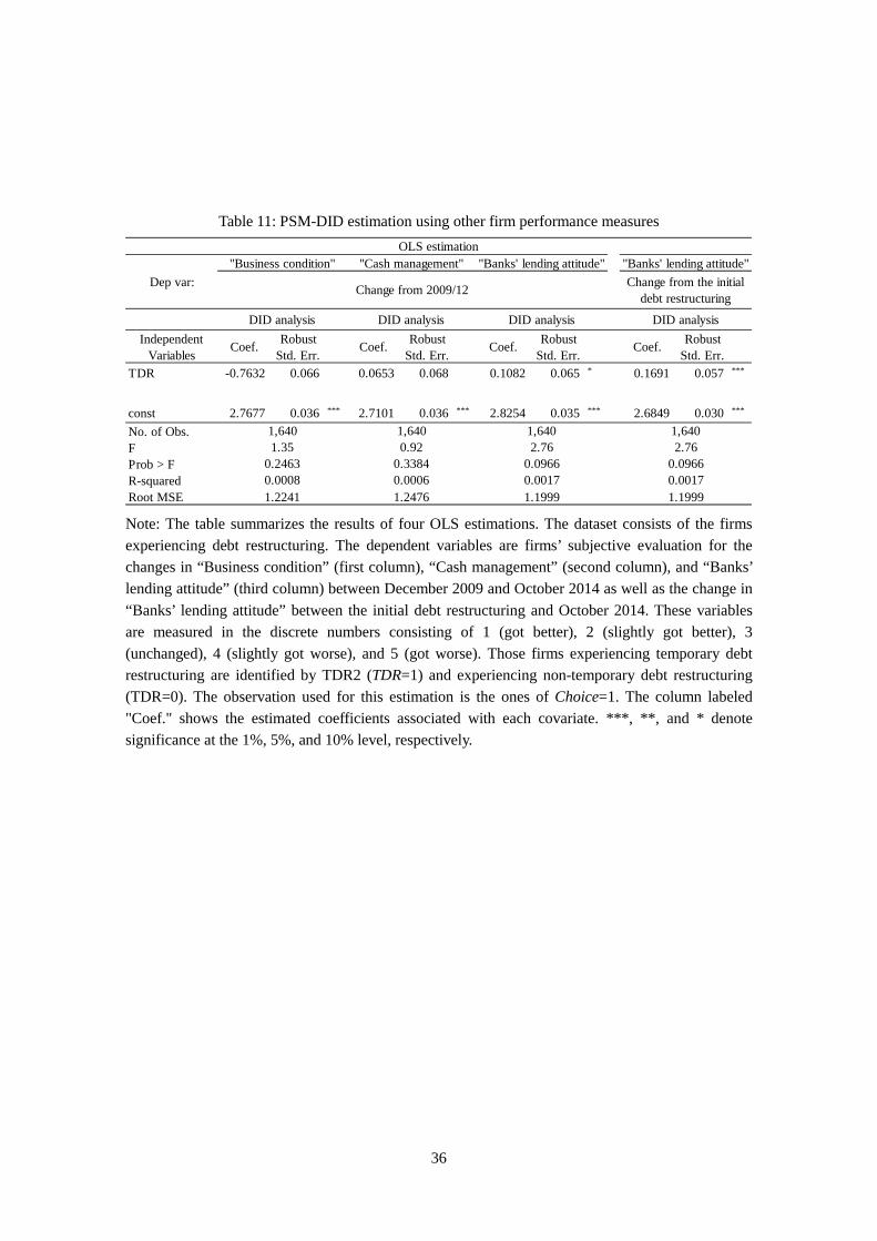
36

Table 11: PSM-DID estimation using other firm performance measures

Note: The table summarizes the results of four OLS estimations. The dataset consists of the firms experiencing debt restructuring. The dependent variables are firms’ subjective evaluation for the changes in “Business condition” (first column), “Cash management” (second column), and “Banks’ lending attitude” (third column) between December 2009 and October 2014 as well as the change in “Banks’ lending attitude” between the initial debt restructuring and October 2014. These variables are measured in the discrete numbers consisting of 1 (got better), 2 (slightly got better), 3 (unchanged), 4 (slightly got worse), and 5 (got worse). Those firms experiencing temporary debt restructuring are identified by TDR2 (TDR=1) and experiencing non-temporary debt restructuring (TDR=0). The observation used for this estimation is the ones of Choice=1. The column labeled "Coef." shows the estimated coefficients associated with each covariate. ***, **, and * denote significance at the 1%, 5%, and 10% level, respectively.

IndependentVariables

Coef. RobustStd. Err.

Coef. RobustStd. Err.

Coef. RobustStd. Err.

Coef. RobustStd. Err.

TDR -0.7632 0.066 0.0653 0.068 0.1082 0.065 * 0.1691 0.057 ***

const 2.7677 0.036 *** 2.7101 0.036 *** 2.8254 0.035 *** 2.6849 0.030 ***

No. of Obs.FProb > FR-squaredRoot MSE 1.1999

Change from 2009/12 Change from the initialdebt restructuring

OLS estimation

Dep var:"Banks' lending attitude"

DID analysis

1,6402.76

0.09660.0017

1.2241 1.2476 1.1999

"Business condition" "Cash management" "Banks' lending attitude"

0.2463 0.3384 0.09660.0008 0.0006 0.0017

1,640 1,640 1,6401.35 0.92 2.76

DID analysis DID analysis DID analysis

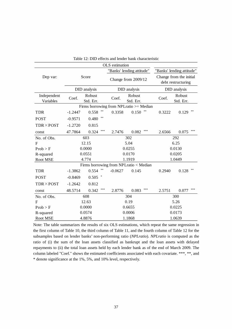
37

Table 12: DID effects and lender bank characteristic

Note: The table summarizes the results of six OLS estimations, which repeat the same regression in the first column of Table 10, the third column of Table 11, and the fourth column of Table 12 for the subsamples based on lender banks’ non-performing ratio (NPLratio). NPLratio is computed as the ratio of (i) the sum of the loan assets classified as bankrupt and the loan assets with delayed repayments to (ii) the total loan assets held by each lender bank as of the end of March 2009. The column labeled "Coef." shows the estimated coefficients associated with each covariate. ***, **, and * denote significance at the 1%, 5%, and 10% level, respectively.

IndependentVariables

Coef. RobustStd. Err.

Coef. RobustStd. Err.

Coef. RobustStd. Err.

TDR -1.2447 0.558 ** 0.3358 0.150 ** 0.3222 0.129 **

POST -0.9571 0.480 **

TDR×POST -1.2720 0.815const 47.7864 0.324 *** 2.7476 0.082 *** 2.6566 0.075 ***

No. of Obs.FProb > FR-squaredRoot MSE

TDR -1.3862 0.554 ** -0.0627 0.145 0.2940 0.128 **

POST -0.8469 0.505 *

TDR×POST -1.2642 0.812const 48.5714 0.342 *** 2.8776 0.083 *** 2.5751 0.077 ***

No. of Obs.FProb > FR-squaredRoot MSE 4.8876 1.1868 1.0639

0.0000 0.6655 0.02250.0574 0.0006 0.0173

608 304 30012.63 0.19 5.26

4.774 1.1919 1.0449

Change from 2009/12ScoreDep var:

Firms borrowing from NPLratio >= Median

Firms borrowing from NPLratio < Median

0.0000 0.0255 0.01300.0551 0.0170 0.0205

603 302 29212.15 5.04 6.25

Change from the initialdebt restructuring

DID analysis DID analysis DID analysis

OLS estimation"Banks' lending attitude" "Banks' lending attitude"