Embed Size (px)
Citation preview
MULTIPLE ITEM INVENTORY MODELS WITH VARIOUS
DEMAND FUNCTIONS AND CONSTRAINTS
Thesis Submitted in partial fulfillment of the requirements for
The award of degree of
Masters of Science
In
Mathematics and Computing
Submitted by
Gaganpreet Kaur
Reg. No.-301303002
Under
the guidance of
Dr. Mahesh Kumar Sharma
July, 2015
School of Mathematics
Thapar University
Patiala-147004(PUNJAB)
INDIA

ABSTRACT
In real situations often inventory manager have to hold thousand of items in an inventory.
In these situations single item inventory models do not help them to manage the inventory
properly. So multi item inventory models are often necessary for the inventory holders. In
today’s market demand of customers is not constant, however it depends on the selling price
and also inventory holders have to face different restrictions like limited space in inventory,
limited investment and restriction on average inventory level. In present work different models
are studied with different demand functions depending on the selling price of items and models
with different constraints.
The whole work is divided into four chapters.
Chapter 1 is introductory in which some classic inventory models have been discussed and
literature related to the work have also been discussed.
In Chapter 2, a review of research paper entitled ”Multi-item EOQ model while demand
is sales price and price break sensitive” studied by Pal et al. (2012) has been reviewed and
some observations have been made.
Based on the observations given in Chapter 2, an attempt has been made in Chapter 3 to
find the solution of such type problems using KT conditions, however in place of the models
considered by Pal et al. (2012), the simple models have been considered.
In Chapter 4, three different multi item inventory models have been solved in which the
objective function is same as in model I of chapter 3 subject to limited warehouse storage,
limited investment on inventory and restriction on average inventory level constraints sepa-
rately.
iii
Contents
CERTIFICATE i
ACKNOWLEDGEMENTS ii
ABSTRACT iii
1 Introduction 1
1.1 Costs Involved In Inventory Problems . . . . . . . . . . . . . . . . . . . . . . . 2
1.2 Basic Economic Order Quantity (EOQ) Model . . . . . . . . . . . . . . . . . . 4
1.3 EOQ Model With Price Breaks . . . . . . . . . . . . . . . . . . . . . . . . . . 6
1.4 Multi-item Inventory Models . . . . . . . . . . . . . . . . . . . . . . . . . . . . 8
1.4.1 Introduction . . . . . . . . . . . . . . . . . . . . . . . . . . . . . . . . . 8
1.4.2 Multi-item EOQ Model With Warehouse Space Constraint . . . . . . . 8
1.4.3 Multi-item EOQ Model with Investment Constraint . . . . . . . . . . . 9
1.4.4 Multi-item EOQ Model with Average Inventory Level Constraint . . . 9
1.5 Present Work . . . . . . . . . . . . . . . . . . . . . . . . . . . . . . . . . . . . 10
1.6 Literature Review . . . . . . . . . . . . . . . . . . . . . . . . . . . . . . . . . . 11
2 Multi-item EOQ Model while Demand is Sales Price and Price Break Sen-
sitive (Review of Research Paper) 16
2.1 Introduction . . . . . . . . . . . . . . . . . . . . . . . . . . . . . . . . . . . . . 16
2.2 Fundamental assumptions and notation . . . . . . . . . . . . . . . . . . . . . . 17
2.2.1 Assumptions . . . . . . . . . . . . . . . . . . . . . . . . . . . . . . . . . 17
2.2.2 Notations . . . . . . . . . . . . . . . . . . . . . . . . . . . . . . . . . . 17
2.3 Mathematical formulation and analysis of the model . . . . . . . . . . . . . . . 17
iv
2.4 Case I . . . . . . . . . . . . . . . . . . . . . . . . . . . . . . . . . . . . . . . . 18
2.5 Case II . . . . . . . . . . . . . . . . . . . . . . . . . . . . . . . . . . . . . . . . 20
2.6 Observations . . . . . . . . . . . . . . . . . . . . . . . . . . . . . . . . . . . . . 22
2.6.1 Case I . . . . . . . . . . . . . . . . . . . . . . . . . . . . . . . . . . . . 22
2.7 Future Scope . . . . . . . . . . . . . . . . . . . . . . . . . . . . . . . . . . . . 23
3 Multi-item Inventory Model with Price Break and Demand Depends on
Selling Price 24
3.1 Introduction . . . . . . . . . . . . . . . . . . . . . . . . . . . . . . . . . . . . . 24
3.2 Mathematical Formulation . . . . . . . . . . . . . . . . . . . . . . . . . . . . . 25
3.3 Model I . . . . . . . . . . . . . . . . . . . . . . . . . . . . . . . . . . . . . . . 25
3.3.1 Case I . . . . . . . . . . . . . . . . . . . . . . . . . . . . . . . . . . . . 25
3.3.2 Numerical Example . . . . . . . . . . . . . . . . . . . . . . . . . . . . . 27
3.3.3 Case II . . . . . . . . . . . . . . . . . . . . . . . . . . . . . . . . . . . . 28
3.3.4 Numerical Example . . . . . . . . . . . . . . . . . . . . . . . . . . . . . 30
3.4 Model II . . . . . . . . . . . . . . . . . . . . . . . . . . . . . . . . . . . . . . . 31
3.4.1 Case I . . . . . . . . . . . . . . . . . . . . . . . . . . . . . . . . . . . . 31
3.4.2 Numerical Example . . . . . . . . . . . . . . . . . . . . . . . . . . . . . 33
3.4.3 Case II . . . . . . . . . . . . . . . . . . . . . . . . . . . . . . . . . . . . 34
3.4.4 Numerical Example . . . . . . . . . . . . . . . . . . . . . . . . . . . . . 36
3.5 Model III . . . . . . . . . . . . . . . . . . . . . . . . . . . . . . . . . . . . . . 36
3.5.1 Case I . . . . . . . . . . . . . . . . . . . . . . . . . . . . . . . . . . . . 36
3.5.2 Numerical Example . . . . . . . . . . . . . . . . . . . . . . . . . . . . . 38
3.5.3 Case II . . . . . . . . . . . . . . . . . . . . . . . . . . . . . . . . . . . . 39
3.5.4 Numerical Example . . . . . . . . . . . . . . . . . . . . . . . . . . . . . 41
3.6 Conclusion . . . . . . . . . . . . . . . . . . . . . . . . . . . . . . . . . . . . . . 42
4 Multi-item Inventory Model in which Demand Depends on Selling Price
under Storage, Investment and Average Inventory Level Constraint. 44
4.1 Introduction . . . . . . . . . . . . . . . . . . . . . . . . . . . . . . . . . . . . . 44
4.2 Mathematical Formulation . . . . . . . . . . . . . . . . . . . . . . . . . . . . . 45
v
4.2.1 Assumptions . . . . . . . . . . . . . . . . . . . . . . . . . . . . . . . . . 45
4.2.2 Notations . . . . . . . . . . . . . . . . . . . . . . . . . . . . . . . . . . 45
4.2.3 Demand and Objective function . . . . . . . . . . . . . . . . . . . . . . 46
4.3 Model I . . . . . . . . . . . . . . . . . . . . . . . . . . . . . . . . . . . . . . . 46
4.3.1 Numerical Example . . . . . . . . . . . . . . . . . . . . . . . . . . . . . 48
4.4 Model II . . . . . . . . . . . . . . . . . . . . . . . . . . . . . . . . . . . . . . . 49
4.4.1 Numerical Example . . . . . . . . . . . . . . . . . . . . . . . . . . . . . 50
4.5 Model III . . . . . . . . . . . . . . . . . . . . . . . . . . . . . . . . . . . . . . 51
4.5.1 Numerical Example . . . . . . . . . . . . . . . . . . . . . . . . . . . . . 53
4.6 Conclusion . . . . . . . . . . . . . . . . . . . . . . . . . . . . . . . . . . . . . . 54
References 55
vi
Chapter 1
Introduction
The word inventory refers to any kind of resource having economic value and is maintained
to fulfil the present and future needs of an organization. Fred Hansman, defined inventory as:
An idle resource of any kind provided such resource has economic value. Each organization
has some type of inventory planning and control system. State and federal governments,
schools, and every manufacturing and production organization are concerned with inventory
planning and control. For example a bank has methods to control its inventory of cash, a
hospital has methods to control blood supplies and medicines etc. Studying how organizations
control their inventory is equivalent to studying how they achieve their objectives by supplying
goods and services to their customers. Inventory control has two major objectives. The first
objective is to maximize the level of customer service by avoiding shortage in stocks. Shortage
in stock causes missed deliveries, backlogged orders, lost sales and unhappy customers. The
second objective of inventory control is to promote efficiency in production or purchasing by
minimizing the purchasing cost along with providing good level of service to the customers.
Many of the classical inventory models concern with single-item model. The multi-item
inventory models are more realistic than the single item model. It is difficult to study an
inventory with multiple items by using classical single item model. Further, in the multi-
item-case main objective is the cost savings, which result from a collective order of several
items. The single-item-models when used for multiple item inventory one item waits until a
certain cost-saving order quantity is reached for other item, and there is a fixed order time
for all items. Most models and software developed or published concentrate on single-item
1
inventory control. However, retailers are responsible for the management of thousands of
items in an inventory and single-item models do not help them to manage large number of
items.
In this chapter classical inventory models have been discussed.
1.1 Costs Involved In Inventory Problems
The costs play an important role in making a decision to maintain the inventory in the
organization. These costs are as follow :
1. Purchasing Cost: Purchasing cost is price of single unit of inventory item. When the
item is offered at a discount if the order size exceeds a certain amount, which is a factor
in deciding how much to order.
2. Holding Cost (Carrying cost): It is the price incurred for carrying (or holding)
inventory items in the stock. This includes the storage cost for providing space to store
the items in inventory, inventory handling cost for payment of salaries to employees and
insurance cost against possible loss from fire or other type of damage.
3. Setup cost (Ordering Cost): Setup cost includes all costs that do not vary with size
of the order but incurred each time an order is placed.
4. Shortage cost: It is the penalty cost when we run out of stock. It includes potential
loss of income and the more subjective cost of loss in customer’s goodwill.
5. Total inventory cost: If price discounts are available, then we should formulate total
inventory cost by taking sum of purchasing cost, Inventory Holding Cost, Shortage Cost
and Setup cost. Thus, the total inventory cost is given by
Total inventory cost=Purchasing Cost + Holding Cost + Setup cost + Shortage cost
When the price discounts are not offered and shortages are not allowed than Total in-
ventory cost is given by
Total inventory cost = Holding Cost + Setup cost
2
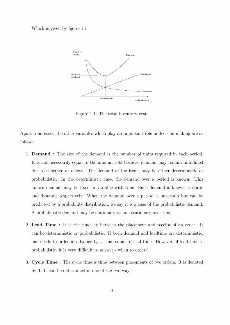
Which is given by figure 1.1
Figure 1.1: The total inventory cost.
Apart from costs, the other variables which play an important role in decision making are as
follows:
1. Demand : The size of the demand is the number of units required in each period.
It is not necessarily equal to the amount sold because demand may remain unfulfilled
due to shortage or delays. The demand of the items may be either deterministic or
probabilistic. In the deterministic case, the demand over a period is known. This
known demand may be fixed or variable with time. Such demand is known as static
and dynamic respectively. When the demand over a period is uncertain but can be
predicted by a probability distribution, we say it is a case of the probabilistic demand.
A probabilistic demand may be stationary or non-stationary over time.
2. Lead Time : It is the time lag between the placement and receipt of an order. It
can be deterministic or probabilistic. If both demand and leadtime are deterministic,
one needs to order in advance by a time equal to lead-time. However, if lead-time is
probabilistic, it is very difficult to answer - when to order?
3. Cycle Time : The cycle time is time between placements of two orders. It is denoted
by T. It can be determined in one of the two ways.
3
(a) Continuous Review : In this case, an order of fixed size is placed every time the
inventory level reaches at a pre-specified level, called reorder level.
(b) Periodic Review : Here the orders are placed at equal interval of time. This is
also called the fixed order interval system.
1.2 Basic Economic Order Quantity (EOQ) Model
EOQ model is one of the oldest and most commonly known techniques. This model was
first developed by Ford Harris and R.Wilson independently in 1915. The objective is to
determine economic order quantity, y which minimizes the total cost of an inventory system
when demand occurs at a constant rate. The model is developed under following assumptions:
1. This model deals with single item.
2. The demand rate is known and constant.
3. Quantity discounts are not available.
4. The ordering cost is constant.
5. Shortages are not allowed and lead time is known and is constant.
6. The inventory holding cost per inventory unit per time unit is known and constant
during the period under review.
4
Notations:
h = Holding cost (Cost per inventory unit per unit time)
y = Order quantity (number of units)
D = Demand rate (units per unit time)
t0 = Ordering cycle length (time units)
K = Setup cost associated with placement of an order (Cost per order)
Where total cost per unit time (TCU) is computed as
TCU(y) = Setup cost per unit time + Holding cost per unit time
=KD
y+
hy
2
The optimum solution that is order quantity y is determined by minimizing TCU(y) with
respect to y. Assuming y is continuous, a necessary condition for finding the optimal value
of y isdTCU(y)
dy= −KD
y2+
h
2= 0
The condition is also sufficient because TCU(y) is a convex function. The solution of the
equation yields the EOQ (i.e economic ordered quantity) y∗ as
y∗ =
√2KD
h(1.1)
Thus, the optimum inventory policy for the model is
Order y∗ =√
2KDh
units after every t∗0 =y∗
Dtime units.
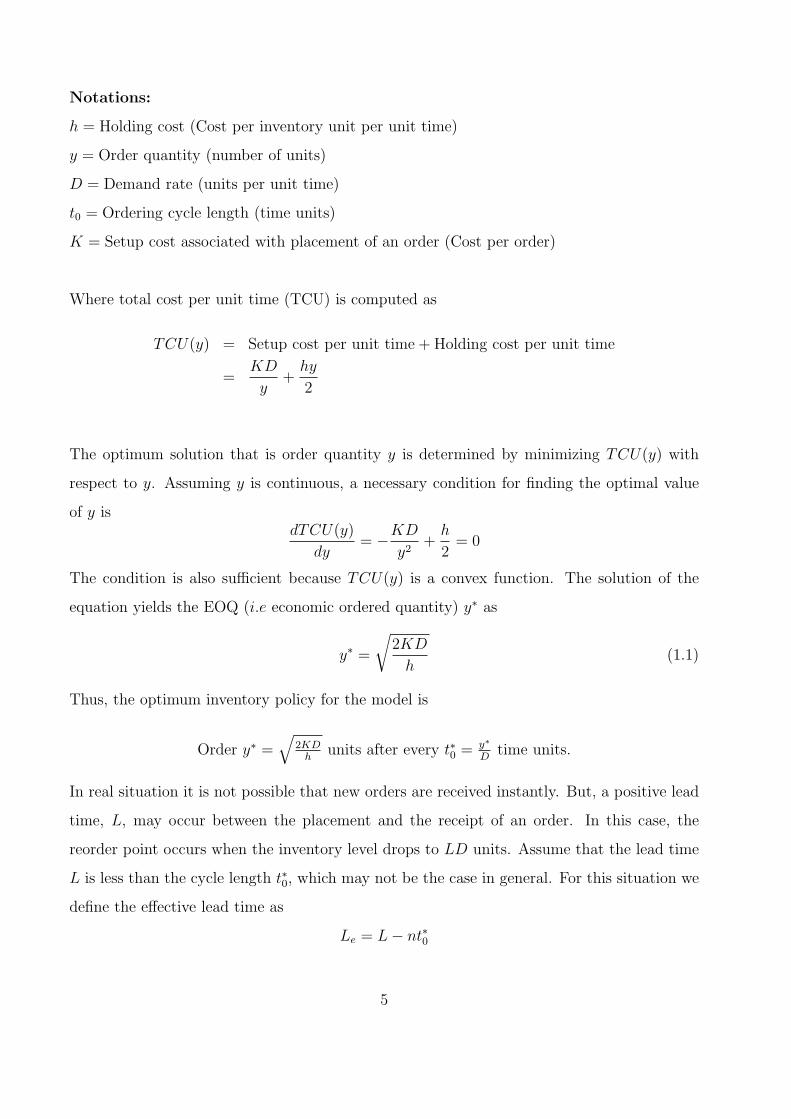
In real situation it is not possible that new orders are received instantly. But, a positive lead
time, L, may occur between the placement and the receipt of an order. In this case, the
reorder point occurs when the inventory level drops to LD units. Assume that the lead time
L is less than the cycle length t∗0, which may not be the case in general. For this situation we
define the effective lead time as
Le = L− nt∗0
5
where n is the largest integer not exceeding Lt∗0. Thus, the reorder point occurs at LeD units,
and the inventory policy can be restated as
Order the quantity y∗ whenever the inventory level drops to LD time units.
Figure 1.2: Reorder points
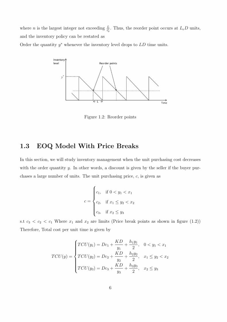
1.3 EOQ Model With Price Breaks
In this section, we will study inventory management when the unit purchasing cost decreases
with the order quantity y. In other words, a discount is given by the seller if the buyer pur-
chases a large number of units. The unit purchasing price, c, is given as
c =
c1, if 0 < y1 < x1
c2, if x1 ≤ y2 < x2
c3, if x2 ≤ y3
s.t c3 < c2 < c1 Where x1 and x2 are limits (Price break points as shown in figure (1.2))
Therefore, Total cost per unit time is given by
TCU(y) =
TCU(y1) = Dc1 +KD
y1+
h1y12
, 0 < y1 < x1
TCU(y2) = Dc2 +KD
y2+
h2y22
, x1 ≤ y2 < x2
TCU(y3) = Dc3 +KD
y3+
h3y32
, x2 ≤ y3
6
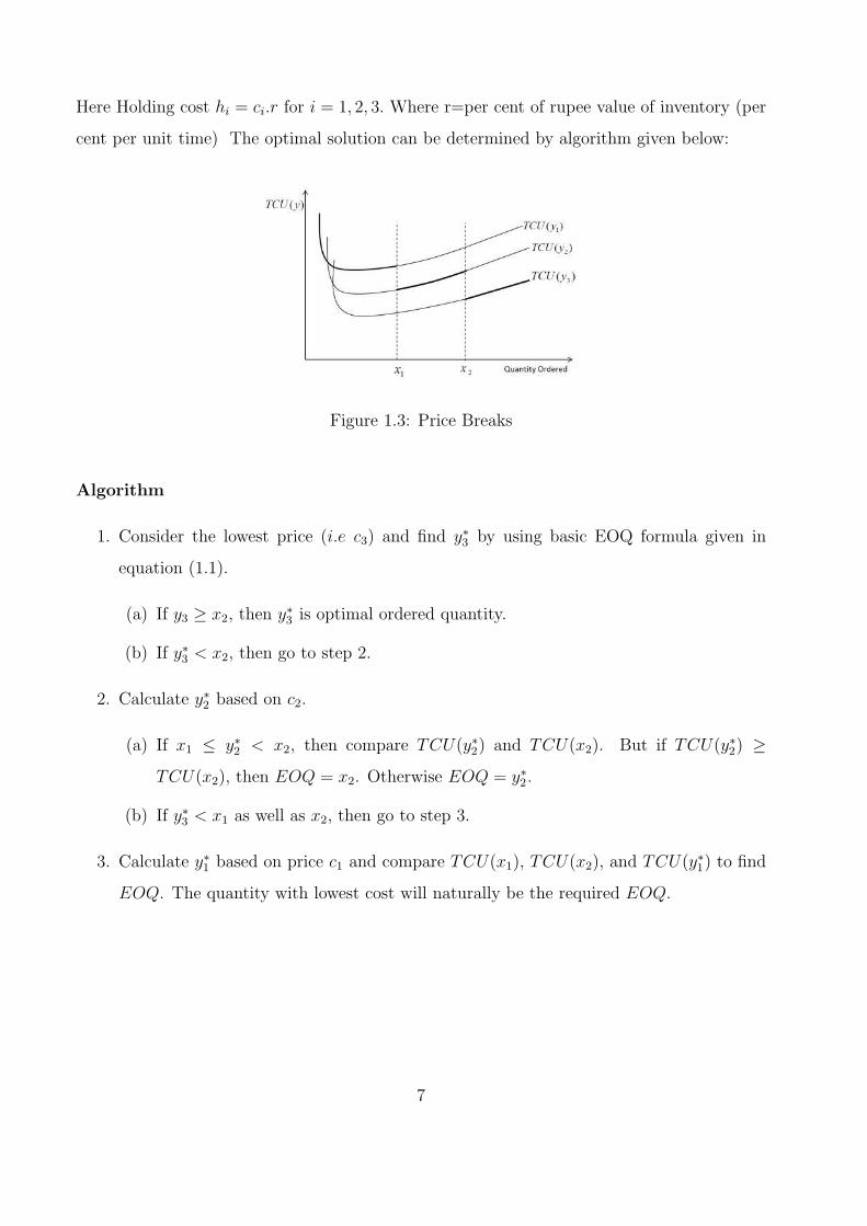
Here Holding cost hi = ci.r for i = 1, 2, 3. Where r=per cent of rupee value of inventory (per
cent per unit time) The optimal solution can be determined by algorithm given below:
Figure 1.3: Price Breaks
Algorithm
1. Consider the lowest price (i.e c3) and find y∗3 by using basic EOQ formula given in
equation (1.1).
(a) If y3 ≥ x2, then y∗3 is optimal ordered quantity.
(b) If y∗3 < x2, then go to step 2.
2. Calculate y∗2 based on c2.
(a) If x1 ≤ y∗2 < x2, then compare TCU(y∗2) and TCU(x2). But if TCU(y∗2) ≥
TCU(x2), then EOQ = x2. Otherwise EOQ = y∗2.
(b) If y∗3 < x1 as well as x2, then go to step 3.
3. Calculate y∗1 based on price c1 and compare TCU(x1), TCU(x2), and TCU(y∗1) to find
EOQ. The quantity with lowest cost will naturally be the required EOQ.
7
1.4 Multi-item Inventory Models
1.4.1 Introduction
In real life there are thousands of items in most of the inventories. In such situations the
single-item models cannot help us to manage the large number of items. Some times a multi-
item model is often necessary, especially when the number of items are very large. A lot
of time and work (and therefore cost) may be saved by using multi-item model. Although
there are, of course, important items which must be studied individually by using single-item
model, but large majority of items (or some less important items) may be dealt with in groups
using multi-item models to save time, work and money.
In this model production or supply is instantaneous with no lead time. Demand is uniform
and deterministic and shortages are not allowed. Define
n = Total number of items in inventory.
fi = Storage area required by the ith item.
W = Total available storage space to all items in the inventory.
Di = Rate of demand for ith item.
Qi = Ordered quantit for ith item.
Ci = Price per unit of item item i.
F = Total investment for all items.
hi = Holding cost for ith item.
Ki = Setup cost for ith item.
1.4.2 Multi-item EOQ Model With Warehouse Space Constraint
In real life situations, a retailer often have limited space for their inventory. Under this con-
straint of limited space they have to take decision about the quantity of all items. So, in this
model we minimize the total inventory cost under the constraint that available storage area
is limited that is if ith item of inventory requires area fi than total area required by the all
inventory items should less than or equal to total available area. Mathematically problem is
given below.
8
Minimize TCU(Q1, Q2, . . . , Qn) =n∑
i=1
[DiKi
Qi
+Qihi
2
]
subject to the space constraint i.e
n∑i=1
fiQi ≤ W
and Qi ≥ 0 for all i = 1, 2, . . . , n.
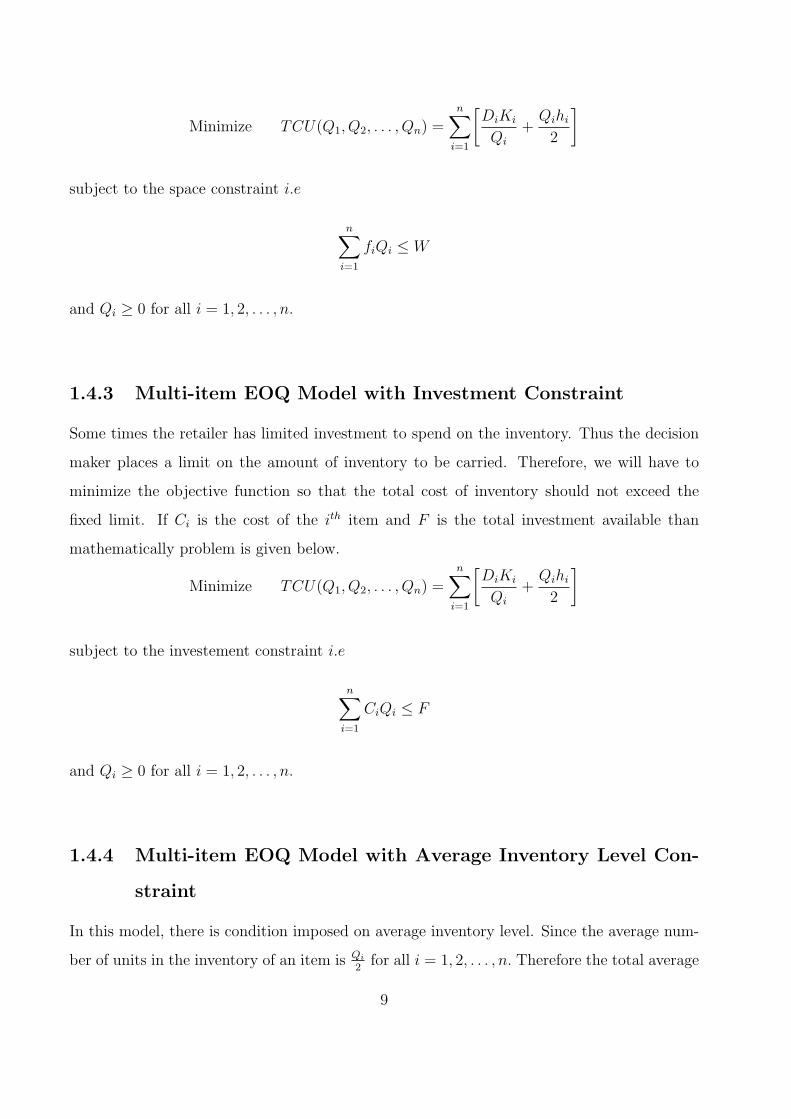
1.4.3 Multi-item EOQ Model with Investment Constraint
Some times the retailer has limited investment to spend on the inventory. Thus the decision
maker places a limit on the amount of inventory to be carried. Therefore, we will have to
minimize the objective function so that the total cost of inventory should not exceed the
fixed limit. If Ci is the cost of the ith item and F is the total investment available than
mathematically problem is given below.
Minimize TCU(Q1, Q2, . . . , Qn) =n∑
i=1
[DiKi
Qi
+Qihi
2
]
subject to the investement constraint i.e
n∑i=1
CiQi ≤ F
and Qi ≥ 0 for all i = 1, 2, . . . , n.
1.4.4 Multi-item EOQ Model with Average Inventory Level Con-
straint
In this model, there is condition imposed on average inventory level. Since the average num-
ber of units in the inventory of an item is Qi
2for all i = 1, 2, . . . , n. Therefore the total average
9
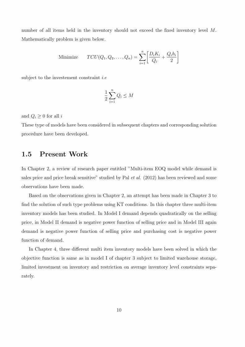
number of all items held in the inventory should not exceed the fixed inventory level M .
Mathematically problem is given below.
Minimize TCU(Q1, Q2, . . . , Qn) =n∑
i=1
[DiKi
Qi
+Qihi
2
]
subject to the investement constraint i.e
1
2
n∑i=1
Qi ≤ M
and Qi ≥ 0 for all i
These type of models have been considered in subsequent chapters and corresponding solution
procedure have been developed.
1.5 Present Work
In Chapter 2, a review of research paper entitled ”Multi-item EOQ model while demand is
sales price and price break sensitive” studied by Pal et al. (2012) has been reviewed and some
observations have been made.
Based on the observations given in Chapter 2, an attempt has been made in Chapter 3 to
find the solution of such type problems using KT conditions. In this chapter three multi-item
inventory models has been studied. In Model I demand depends quadratically on the selling
price, in Model II demand is negative power function of selling price and in Model III again
demand is negative power function of selling price and purchasing cost is negative power
function of demand.
In Chapter 4, three different multi item inventory models have been solved in which the
objective function is same as in model I of chapter 3 subject to limited warehouse storage,
limited investment on inventory and restriction on average inventory level constraints sepa-
rately.
10
1.6 Literature Review
Inventory theory deals with the management of stock levels with the aim that demand for
these items is met. Most of the models are developed to answer the two questions, first one
is when an order should be placed? and the second is what ordered quantity should be? A
lot of single items models had been developed till the date based on different assumptions
like variable or probabilistic demand, zero-lead time lost sales and back ordering assumptions
when in inventory demand exceeds supply etc. Wang [22] presented a model where he defined
an appropriate time-dependent partial backlogging rate and introduces the opportunity cost
due to lost sales. The effects of changes in the backlogging parameter and unit opportunity
cost on the optimal total cost have been studied and optimal number of replenishment was
carried out. Later on Wee et al. [19] presents a modified method to compute economic order
quantities without derivatives by cost-difference comparisons. Extensions to allow the back
orders were done for EOQ/EPQ models. Limiting values on a finite planning horizon were
used rather than algebraic manipulations for the cost function comparisons. They used the
cost-difference comparisons between two consecutive batch numbers for a finite horizon and
the variable of batch size to express cost function rather than cycle length. The convergence
of optimal batch size is derived rather than optimal cycle length. For the models with back-
orders, they used fill rate to express the proportion with positive inventory in a cycle length.
Sana [18] presented an EOQ model over an infinite horizon for perishable items where demand
was price dependent and partial backorder permitted. The rate of deterioration was taken to
be time proportional and its was assumed that shortage occurs at starting inventory cycle.
It is assumed that the demand rate is price dependent and the deterioration rate is taken
to be time proportional. The SFI (Shortage Followed by Inventory) of replenishment is fol-
lowed. An analytical optimal solution of the integrated average profit function was discussed
for various partial backlogging issues. Also, new functions of price-dependent demand and
deterioration have been introduced and the analysis of optimal solution have been done from
general profit function. Finally, the optimal solution of the integrated profit function was
discussed with appropriate numerical examples. The author developed the criterion for the
optimal solution for the replenishment schedule , and proved that the optimal ordering policy
11
is unique.
Sana [4] developed a finite time-horizon deterministic EOQ (Economic Order Quantity) model
where the rate of demand decreases quadratically with selling price. Prices at different pe-
riods were considered as decision variables. The objective was to find the optimal ordering
quantity and optimal sales prices that maximizes the vendors total profit. The author divides
the time horizon into n equal periods with n different prices which were decision variables. A
profit function has been formulated which has been maximized analytically.
Inventory control problems in real world usually involve multiple products. Multi item in-
ventory models are often necessary for inventories holding thousand of items as studied by
Lenard and Roy [25] presented the difficulties encountered in the practice of inventory control.
It led to the conclusion that a large gap exists between theory and practice in inventory man-
agement. They presents the multi-item inventory control by defining the concepts of families
and aggregate items. In inventory control there may be a large number of objectives, the
most important ones generally concerning the overall service level and the average quantity
of items held in stock. These objectives are naturally not determined at the item level but at
a higher level where a large number of items are concerned. The author studied that single-
item models are not appropriate to this type of management. It is only with a multi-item
inventory model able to give a overview of the system that objectives may be set and that
policies may be determined with respect to the objectives. Moreover, a lot of time and work
(and therefore cost) may be saved by coordinating policies for the different items. Although
there are, of course, important items which must be studied individually, large majority of
items may be dealt with in groups.
Two item inventory model for deteriorating items with a linear stock dependent demand
has been studied by Bhattacharya [9]. Classical inventory models generally dealt with a
single-item. But in real world situation, a single-item inventory seldom occurs. It is a com-
mon experience that the presence of a second item in an inventory favors the demand of the
first and vice-versa; the effect may be different in the two cases. This is why; the companies
12
or the retailers deal with several items and stock them in their showrooms/warehouses. This
leads to the idea of a multi-item inventory. Further author showed that from linear demand
rate, it follows that more is the inventory, more is demand. They also mentioned that un-
der proper restrictions on the model, a steady state optimal solution can always be calculated.
Haksever and Moussourakis [12] presented a mixed-integer programming model to optimize
the two fundamental decisions of inventory management that is how much to order and when
to order for ordering multiple inventory items subject to multiple resource constraints. It also
determines whether a fixed cycle for all products or an independent cycle for each should be
used for a lower total cost.
Brandimarte [16] considered a stochastic version of the classical multi-item capacitated lot
sizing problem. Demand uncertainty was explicitly modeled through a scenario tree, result-
ing in a multi-stage mixed integer stochastic programming model with resource. The author
proposed a plant-location-based model formulation and a heuristic solution approach based
on a fix-and-relax strategy.
A multi-item EOQ model is developed by Sana [11] when the time varying demand is in-
fluenced by enterprises initiatives like advertising media and salesmen effort. He developed a
model for deteriorating and ameliorating items with capacity constraint for storage facility.
The effect of inflation and time value of money in the profit, cost parameter and associated
profit was also considered. The associated profit function was maximized by Euler-Lagrange’s
method and it was illustrated by varying demands like quadratic, linear and exponential de-
mand functions. The model provides the major contribution on the effect of advertising and
salesmen’s initiatives on demand - to operations in management practice.
Zhang [10] considered the multi-product newsboy problem with both supplier quantity dis-
counts and a budget constraint, while each feature has been addressed separately. Different
from most previous nonlinear optimization models on the topic, the problem was formulated
13
as a mixed integer nonlinear programming model due to price discounts. A Lagrangian relax-
ation approach is presented to solve the problem. The purpose of this study was to investigate
the affect of both a budget constraint and supplier quantity discounts on the optimal order
quantities in a multi-product newsboy problem.
Kotab and Fergany [14] derived the analytical solution of the EOQ model of multiple items
with both demand-dependent unit cost and leading time using geometric programming ap-
proach. The varying purchase and leading time crashing costs were considered to be con-
tinuous functions of demand rate and leading time, respectively. The aim of this study was
to derive the optimal solution policy of EOQ inventory model and minimize the total cost
function based on the values of demand rate, order quantity and leading time using geometric
programming technique.
Pal et al. [7] studied a three-layer multi-item supply chain involving multiple suppliers,
manufacturer and multiple retailers where each finished product is produced by the combina-
tion of the fixed percentage of various types of raw materials and each raw material supplier
can supply only one material. Here, they consider that the manufacturer delivers finished
products to the multiple retailers where each of the retailers sells their multiple products
according to their demand in the market. Overall, the total integrated profit of the supply
chain is evaluated and is optimized with respect to ordering lot sizes of the raw materials.
A multi-item deterministic economic order quantity model is developed by Pal et al. [3]
for a retailer. They assumed that the demand rate of the items decreases quadratically with
increase in selling price and increases exponentially with increase in level of price breaks.
They have considered a restriction on level of price breaks. In this paper, according to the
level of price break retailer (or inventory manager) gives discount on selling price of items to
customer. If the total selling price of retail mall at any time t is more than the level of price
breaks, then the retailer gives discount on selling price to customers. The author formulated
a maximizing profit model by considering selling prices, ordering quantities of products and
level of price breaks as decision variables with respect to the restriction on total selling price
14
at any time t.
Barron and Sana [6] proposed an economic order quantity inventory model of multi-items
in a two-layer supply chain where demand is sensitive to promotional effort. In this inventory
model, the supplier offerd a delay period to the retailer for paying the outstanding amount
of the purchasing cost for the finished products. The profit functions of the supplier and
the retailer were formulated by considering the setup cost, holding cost, selling price, and
promotional costs. They also compared collaborative and non-collaborative systems in terms
of their average profits.
15
Chapter 2
Multi-item EOQ Model while Demand
is Sales Price and Price Break
Sensitive (Review of Research Paper)
2.1 Introduction
Pal et al. (2012) developed a multi-item deterministic economic order quantity model for
a retailer. It is assumed that the demand rate of the items decreases quadratically with
increase in selling price and increases exponentially with increase in level of price breaks with
a restriction on level of price breaks. In this model, according to the level of price break
retailer (or inventory manager) gives discount on selling price of items to customer. If the
total selling price of retailer is more than the level of price breaks, then the retailer gives
discount on selling price to customers. The author formulated a maximizing profit model by
considering selling prices, ordering quantities of products and level of price breaks as decision
variables with respect to the restriction on total selling price. The model is solved by using the
method of Lagrangian multiplier. In this chapter above mentioned paper has been reviewed
and some observations have been made and an attempt has been made to rewrite some of the
expressions.
16
2.2 Fundamental assumptions and notation
2.2.1 Assumptions
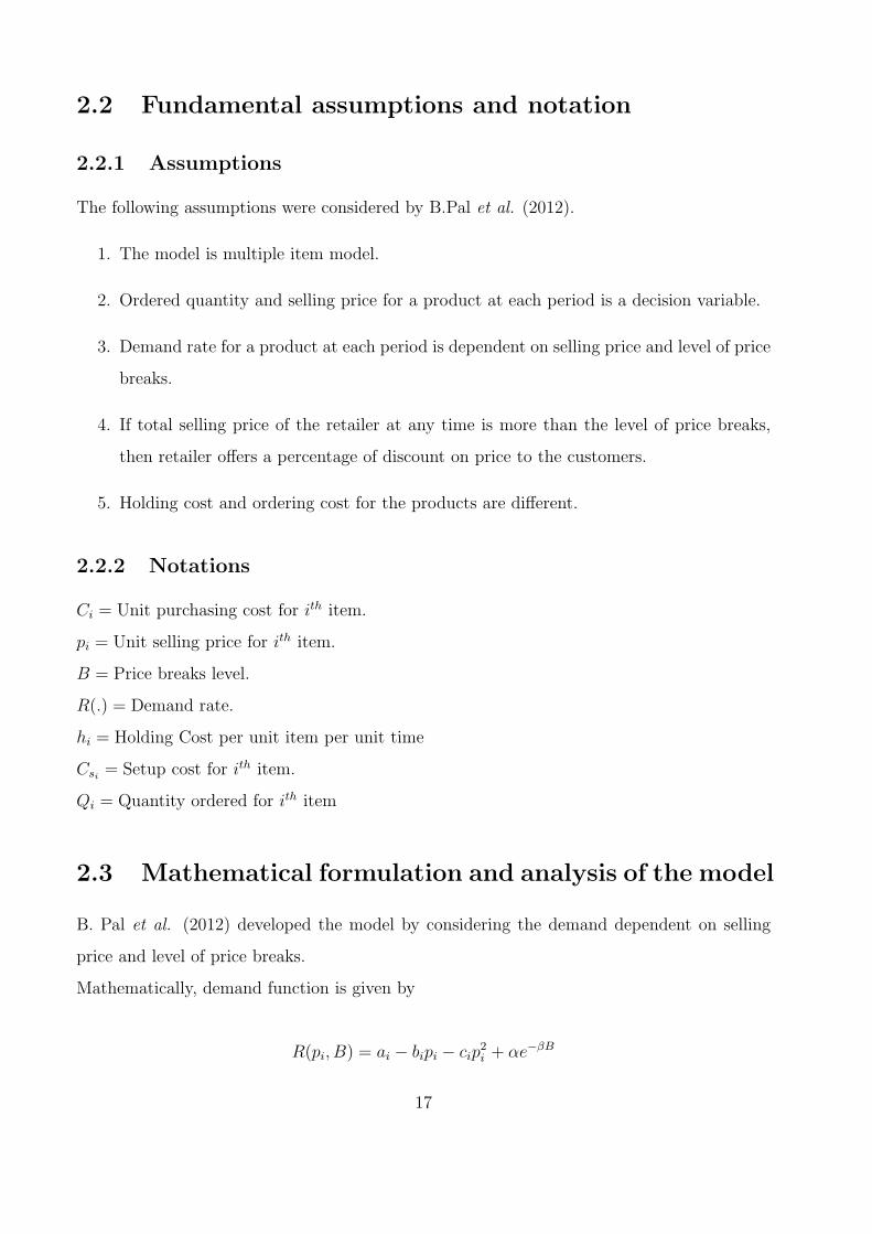
The following assumptions were considered by B.Pal et al. (2012).
1. The model is multiple item model.
2. Ordered quantity and selling price for a product at each period is a decision variable.
3. Demand rate for a product at each period is dependent on selling price and level of price
breaks.
4. If total selling price of the retailer at any time is more than the level of price breaks,
then retailer offers a percentage of discount on price to the customers.
5. Holding cost and ordering cost for the products are different.
2.2.2 Notations
Ci = Unit purchasing cost for ith item.
pi = Unit selling price for ith item.
B = Price breaks level.
R(.) = Demand rate.
hi = Holding Cost per unit item per unit time
Csi = Setup cost for ith item.
Qi = Quantity ordered for ith item
2.3 Mathematical formulation and analysis of the model
B. Pal et al. (2012) developed the model by considering the demand dependent on selling
price and level of price breaks.
Mathematically, demand function is given by
R(pi, B) = ai − bipi − cip2i + αe−βB
17
where ai, bi, ci, α, β are all suitable positive constants and ai >> bi >> ci for i = 1, 2, . . . , n.
The total profit has been maximized with respect to discount criteria. Retailer offered discount
to the customers on the basis that wether selling price crosses the price break level or not.
According to this, the model was divided in the following two cases.
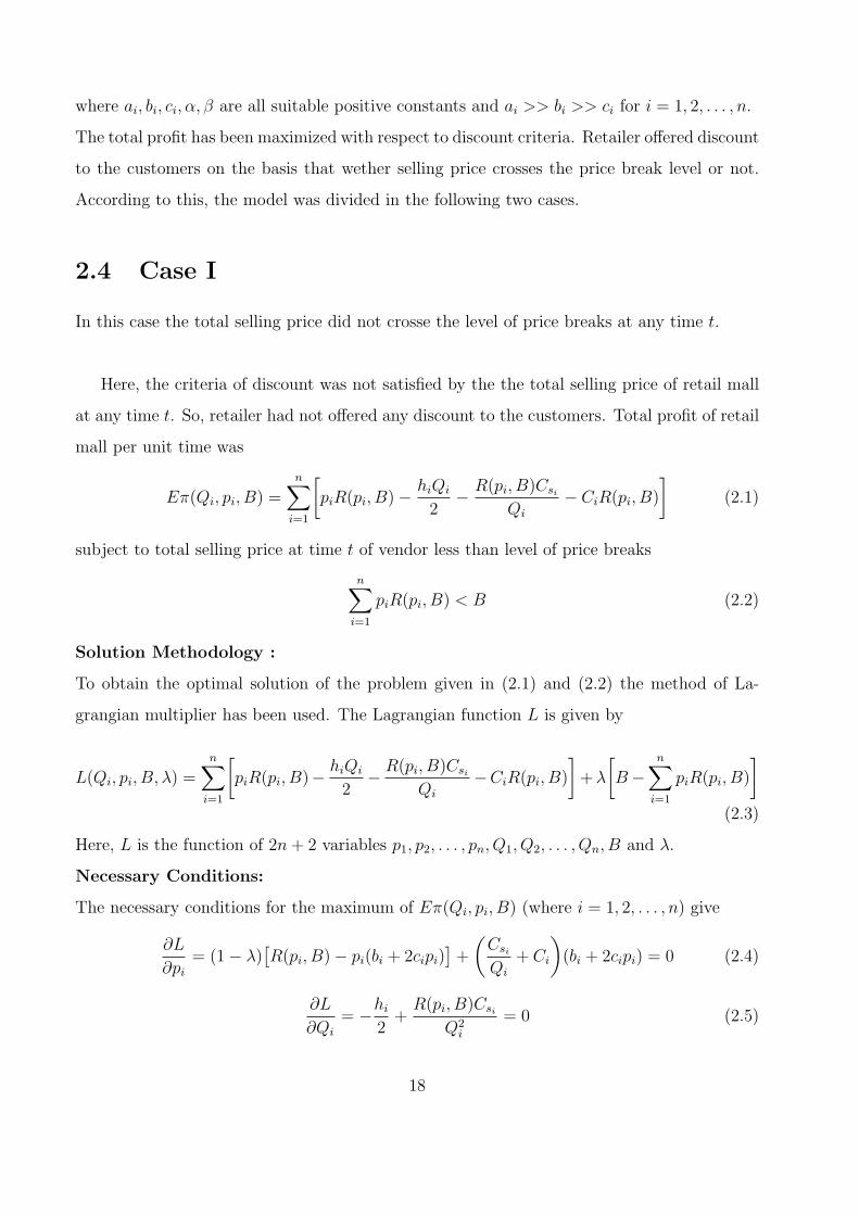
2.4 Case I
In this case the total selling price did not crosse the level of price breaks at any time t.
Here, the criteria of discount was not satisfied by the the total selling price of retail mall
at any time t. So, retailer had not offered any discount to the customers. Total profit of retail
mall per unit time was
Eπ(Qi, pi, B) =n∑
i=1
[piR(pi, B)− hiQi
2− R(pi, B)Csi
Qi
− CiR(pi, B)
](2.1)
subject to total selling price at time t of vendor less than level of price breaks
n∑i=1
piR(pi, B) < B (2.2)
Solution Methodology :
To obtain the optimal solution of the problem given in (2.1) and (2.2) the method of La-
grangian multiplier has been used. The Lagrangian function L is given by
L(Qi, pi, B, λ) =n∑
i=1
[piR(pi, B)− hiQi
2− R(pi, B)Csi
Qi
−CiR(pi, B)
]+λ
[B−
n∑i=1
piR(pi, B)
](2.3)
Here, L is the function of 2n+ 2 variables p1, p2, . . . , pn, Q1, Q2, . . . , Qn, B and λ.
Necessary Conditions:
The necessary conditions for the maximum of Eπ(Qi, pi, B) (where i = 1, 2, . . . , n) give
∂L
∂pi= (1− λ)
[R(pi, B)− pi(bi + 2cipi)
]+
(Csi
Qi
+ Ci
)(bi + 2cipi) = 0 (2.4)
∂L
∂Qi
= −hi
2+
R(pi, B)Csi
Q2i
= 0 (2.5)
18
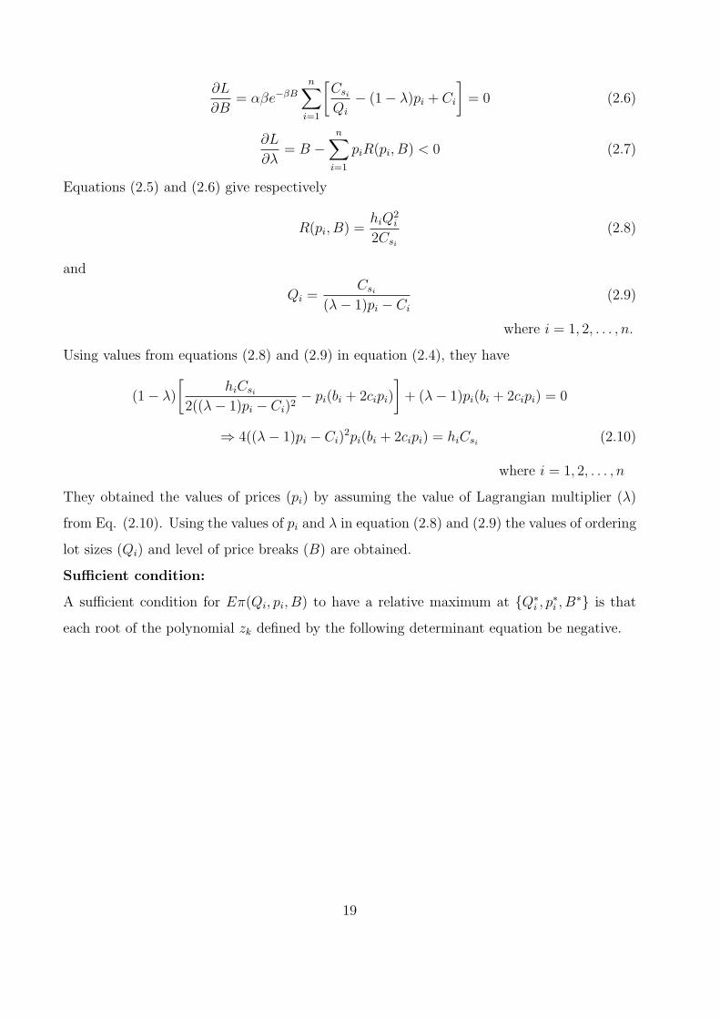
∂L
∂B= αβe−βB
n∑i=1
[Csi
Qi
− (1− λ)pi + Ci
]= 0 (2.6)
∂L
∂λ= B −
n∑i=1
piR(pi, B) < 0 (2.7)
Equations (2.5) and (2.6) give respectively
R(pi, B) =hiQ
2i
2Csi
(2.8)
and
Qi =Csi
(λ− 1)pi − Ci
(2.9)
where i = 1, 2, . . . , n.
Using values from equations (2.8) and (2.9) in equation (2.4), they have
(1− λ)
[hiCsi
2((λ− 1)pi − Ci)2− pi(bi + 2cipi)
]+ (λ− 1)pi(bi + 2cipi) = 0
⇒ 4((λ− 1)pi − Ci)2pi(bi + 2cipi) = hiCsi (2.10)
where i = 1, 2, . . . , n
They obtained the values of prices (pi) by assuming the value of Lagrangian multiplier (λ)
from Eq. (2.10). Using the values of pi and λ in equation (2.8) and (2.9) the values of ordering
lot sizes (Qi) and level of price breaks (B) are obtained.
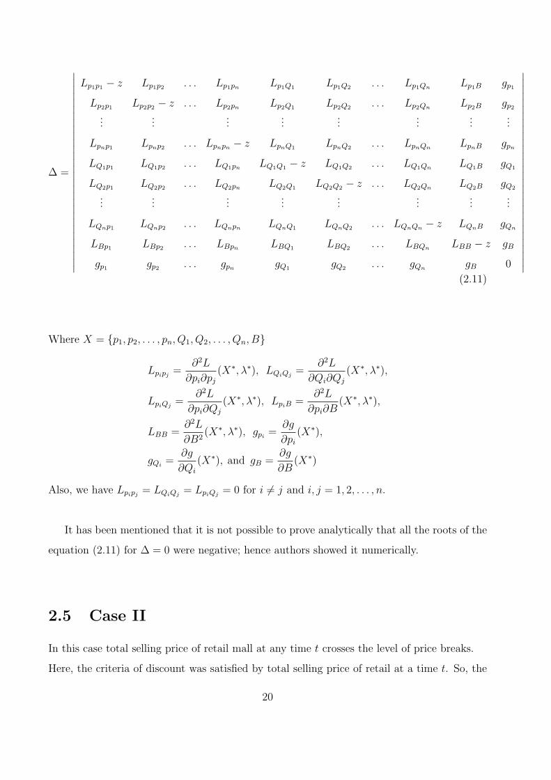
Sufficient condition:
A sufficient condition for Eπ(Qi, pi, B) to have a relative maximum at {Q∗i , p
∗i , B
∗} is that
each root of the polynomial zk defined by the following determinant equation be negative.
19
∆ =
∣∣∣∣∣∣∣∣∣∣∣∣∣∣∣∣∣∣∣∣∣∣∣∣∣∣∣∣∣∣
Lp1p1 − z Lp1p2 . . . Lp1pn Lp1Q1 Lp1Q2 . . . Lp1Qn Lp1B gp1
Lp2p1 Lp2p2 − z . . . Lp2pn Lp2Q1 Lp2Q2 . . . Lp2Qn Lp2B gp2...
......
......
......
...
Lpnp1 Lpnp2 . . . Lpnpn − z LpnQ1 LpnQ2 . . . LpnQn LpnB gpn
LQ1p1 LQ1p2 . . . LQ1pn LQ1Q1 − z LQ1Q2 . . . LQ1Qn LQ1B gQ1
LQ2p1 LQ2p2 . . . LQ2pn LQ2Q1 LQ2Q2 − z . . . LQ2Qn LQ2B gQ2
......
......
......
......
LQnp1 LQnp2 . . . LQnpn LQnQ1 LQnQ2 . . . LQnQn − z LQnB gQn
LBp1 LBp2 . . . LBpn LBQ1 LBQ2 . . . LBQn LBB − z gB
gp1 gp2 . . . gpn gQ1 gQ2 . . . gQn gB 0
∣∣∣∣∣∣∣∣∣∣∣∣∣∣∣∣∣∣∣∣∣∣∣∣∣∣∣∣∣∣(2.11)
Where X = {p1, p2, . . . , pn, Q1, Q2, . . . , Qn, B}
Lpipj =∂2L
∂pi∂pj(X∗, λ∗), LQiQj
=∂2L
∂Qi∂Qj
(X∗, λ∗),
LpiQj=
∂2L
∂pi∂Qj
(X∗, λ∗), LpiB =∂2L
∂pi∂B(X∗, λ∗),
LBB =∂2L
∂B2(X∗, λ∗), gpi =
∂g
∂pi(X∗),
gQi=
∂g
∂Qi
(X∗), and gB =∂g
∂B(X∗)
Also, we have Lpipj = LQiQj= LpiQj
= 0 for i ̸= j and i, j = 1, 2, . . . , n.
It has been mentioned that it is not possible to prove analytically that all the roots of the
equation (2.11) for ∆ = 0 were negative; hence authors showed it numerically.
2.5 Case II
In this case total selling price of retail mall at any time t crosses the level of price breaks.
Here, the criteria of discount was satisfied by total selling price of retail at a time t. So, the
20
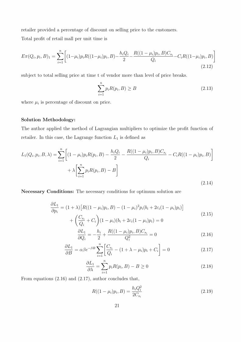
retailer provided a percentage of discount on selling price to the customers.
Total profit of retail mall per unit time is
Eπ(Qi, pi, B)1 =n∑
i=1
[(1−µi)piR((1−µi)pi, B)−hiQi
2−R((1− µi)pi, B)Csi
Qi
−CiR((1−µi)pi, B)
](2.12)
subject to total selling price at time t of vendor more than level of price breaks.
n∑i=1
piR(pi, B) ≥ B (2.13)
where µi is percentage of discount on price.
Solution Methodology:
The author applied the method of Lagrangian multipliers to optimize the profit function of
retailer. In this case, the Lagrange function L1 is defined as
L1(Qi, pi, B, λ) =n∑
i=1
[(1− µi)piR(pi, B)− hiQi
2− R((1− µi)pi, B)Csi
Qi
− CiR((1− µi)pi, B)
]+ λ
[ n∑i=1
piR(pi, B)−B
](2.14)
Necessary Conditions: The necessary conditions for optimum solution are
∂L1
∂pi= (1 + λ)
[R((1− µi)pi, B)− (1− µi)
2pi(bi + 2ci(1− µi)pi)]
+
(Csi
Qi
+ Ci
)(1− µi)(bi + 2ci(1− µi)pi) = 0
(2.15)
∂L1
∂Qi
= −hi
2+
R((1− µi)pi, B)Csi
Q2i
= 0 (2.16)
∂L1
∂B= αβe−βB
n∑i=1
[Csi
Qi
− (1 + λ− µi)pi + Ci
]= 0 (2.17)
∂L1
∂λ=
n∑i=1
piR(pi, B)−B ≥ 0 (2.18)
From equations (2.16) and (2.17), author concludes that,
R((1− µi)pi, B) =hiQ
2i
2Csi
(2.19)
21
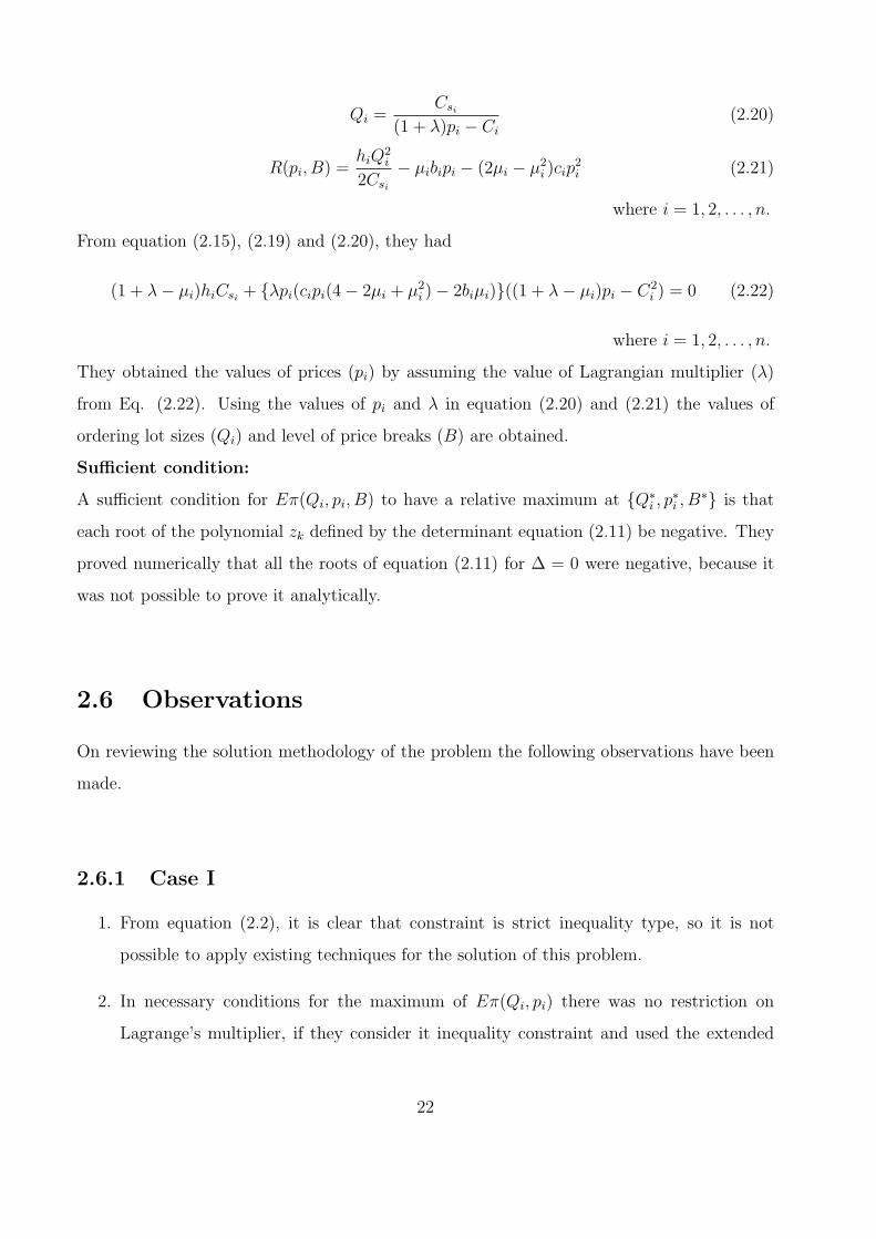
Qi =Csi
(1 + λ)pi − Ci
(2.20)
R(pi, B) =hiQ
2i
2Csi
− µibipi − (2µi − µ2i )cip
2i (2.21)
where i = 1, 2, . . . , n.
From equation (2.15), (2.19) and (2.20), they had
(1 + λ− µi)hiCsi + {λpi(cipi(4− 2µi + µ2i )− 2biµi)}((1 + λ− µi)pi − C2
i ) = 0 (2.22)
where i = 1, 2, . . . , n.
They obtained the values of prices (pi) by assuming the value of Lagrangian multiplier (λ)
from Eq. (2.22). Using the values of pi and λ in equation (2.20) and (2.21) the values of
ordering lot sizes (Qi) and level of price breaks (B) are obtained.
Sufficient condition:
A sufficient condition for Eπ(Qi, pi, B) to have a relative maximum at {Q∗i , p
∗i , B
∗} is that
each root of the polynomial zk defined by the determinant equation (2.11) be negative. They
proved numerically that all the roots of equation (2.11) for ∆ = 0 were negative, because it
was not possible to prove it analytically.
2.6 Observations
On reviewing the solution methodology of the problem the following observations have been
made.
2.6.1 Case I
1. From equation (2.2), it is clear that constraint is strict inequality type, so it is not
possible to apply existing techniques for the solution of this problem.
2. In necessary conditions for the maximum of Eπ(Qi, pi) there was no restriction on
Lagrange’s multiplier, if they consider it inequality constraint and used the extended
22
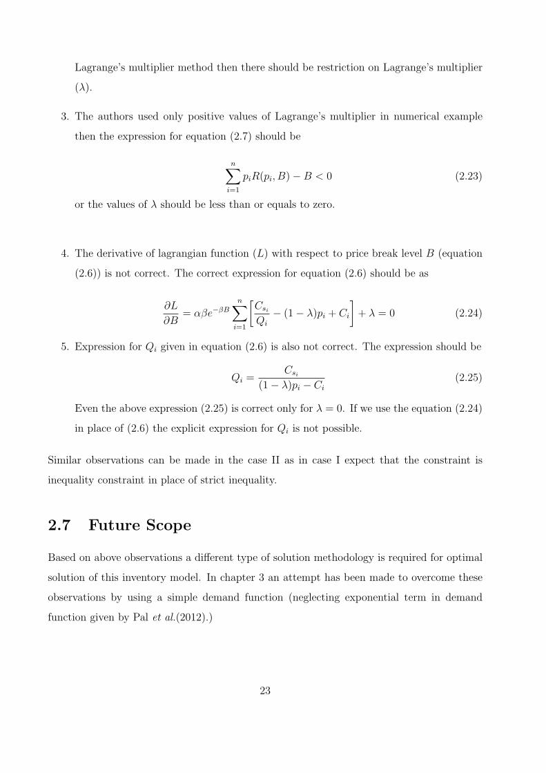
Lagrange’s multiplier method then there should be restriction on Lagrange’s multiplier
(λ).
3. The authors used only positive values of Lagrange’s multiplier in numerical example
then the expression for equation (2.7) should be
n∑i=1
piR(pi, B)−B < 0 (2.23)
or the values of λ should be less than or equals to zero.
4. The derivative of lagrangian function (L) with respect to price break level B (equation
(2.6)) is not correct. The correct expression for equation (2.6) should be as
∂L
∂B= αβe−βB
n∑i=1
[Csi
Qi
− (1− λ)pi + Ci
]+ λ = 0 (2.24)
5. Expression for Qi given in equation (2.6) is also not correct. The expression should be
Qi =Csi
(1− λ)pi − Ci
(2.25)
Even the above expression (2.25) is correct only for λ = 0. If we use the equation (2.24)
in place of (2.6) the explicit expression for Qi is not possible.
Similar observations can be made in the case II as in case I expect that the constraint is
inequality constraint in place of strict inequality.
2.7 Future Scope
Based on above observations a different type of solution methodology is required for optimal
solution of this inventory model. In chapter 3 an attempt has been made to overcome these
observations by using a simple demand function (neglecting exponential term in demand
function given by Pal et al.(2012).)
23
Chapter 3
Multi-item Inventory Model with
Price Break and Demand Depends on
Selling Price
3.1 Introduction
In chapter 2 a multi-item EOQ model ”Multi-item EOQ model while demand is sales price and
price break sensitive” has been discussed and some observations have been made on solution
methodology given by Pal et al. (2012). Based on those observations an attempt has been
made to find the optimal solution of such type of problems using KT conditions. However
in place of the model considered by Pal et al. (2012) a simple model has been considered in
which exponential term in demand function is neglected. In this chapter we considered the
following three models.
In the first model it has been considered that demand of customers depends quadratically
on the selling price only and the price break is fixed.
In second model, the demand is dependent as negative power function on the selling price
only and the price break is fixed. The demand of customers decreases the negative power of
selling price with increase in it.
In third model, again demand is dependent on selling price as negative power function of
it and the purchasing cost price is dependent as the negative power function of demand.
24
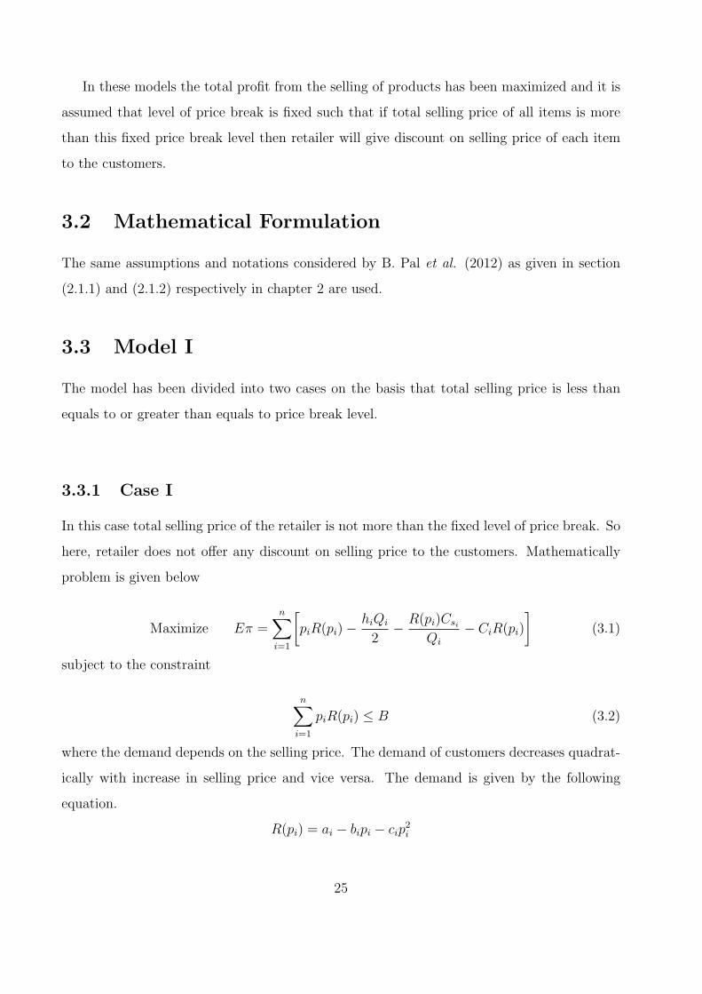
In these models the total profit from the selling of products has been maximized and it is
assumed that level of price break is fixed such that if total selling price of all items is more
than this fixed price break level then retailer will give discount on selling price of each item
to the customers.
3.2 Mathematical Formulation
The same assumptions and notations considered by B. Pal et al. (2012) as given in section
(2.1.1) and (2.1.2) respectively in chapter 2 are used.
3.3 Model I
The model has been divided into two cases on the basis that total selling price is less than
equals to or greater than equals to price break level.
3.3.1 Case I
In this case total selling price of the retailer is not more than the fixed level of price break. So
here, retailer does not offer any discount on selling price to the customers. Mathematically
problem is given below
Maximize Eπ =n∑
i=1
[piR(pi)−
hiQi
2− R(pi)Csi
Qi
− CiR(pi)
](3.1)
subject to the constraint
n∑i=1
piR(pi) ≤ B (3.2)
where the demand depends on the selling price. The demand of customers decreases quadrat-
ically with increase in selling price and vice versa. The demand is given by the following
equation.
R(pi) = ai − bipi − cip2i
25
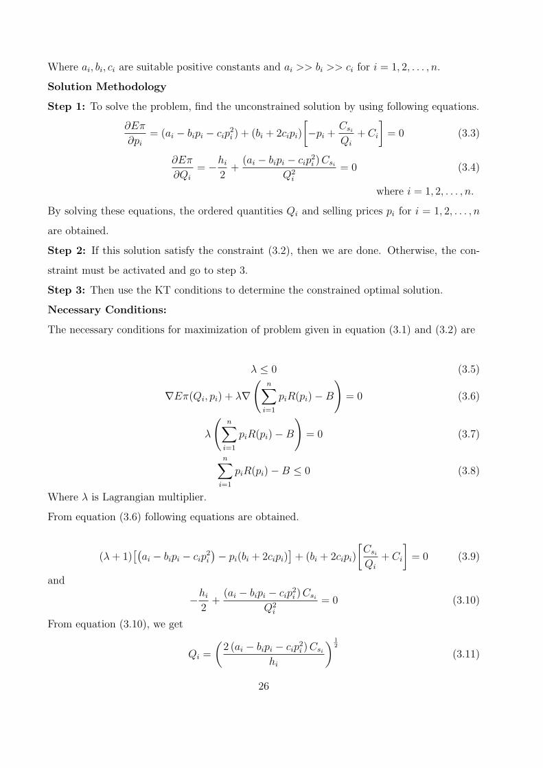
Where ai, bi, ci are suitable positive constants and ai >> bi >> ci for i = 1, 2, . . . , n.
Solution Methodology
Step 1: To solve the problem, find the unconstrained solution by using following equations.
∂Eπ
∂pi= (ai − bipi − cip
2i ) + (bi + 2cipi)
[−pi +
Csi
Qi
+ Ci
]= 0 (3.3)
∂Eπ
∂Qi
= −hi
2+
(ai − bipi − cip2i )Csi
Q2i
= 0 (3.4)
where i = 1, 2, . . . , n.
By solving these equations, the ordered quantities Qi and selling prices pi for i = 1, 2, . . . , n
are obtained.
Step 2: If this solution satisfy the constraint (3.2), then we are done. Otherwise, the con-
straint must be activated and go to step 3.
Step 3: Then use the KT conditions to determine the constrained optimal solution.
Necessary Conditions:
The necessary conditions for maximization of problem given in equation (3.1) and (3.2) are
λ ≤ 0 (3.5)
∇Eπ(Qi, pi) + λ∇
(n∑
i=1
piR(pi)−B
)= 0 (3.6)
λ
(n∑
i=1
piR(pi)−B
)= 0 (3.7)
n∑i=1
piR(pi)−B ≤ 0 (3.8)
Where λ is Lagrangian multiplier.
From equation (3.6) following equations are obtained.
(λ+ 1)[(ai − bipi − cip
2i
)− pi(bi + 2cipi)
]+ (bi + 2cipi)
[Csi
Qi
+ Ci
]= 0 (3.9)
and
−hi
2+
(ai − bipi − cip2i )Csi
Q2i
= 0 (3.10)
From equation (3.10), we get
Qi =
(2 (ai − bipi − cip
2i )Csi
hi
) 12
(3.11)
26
From equations (3.11) and (3.9), we get
(λ+ 1)[(ai − bipi − cip
2i
)− pi(bi + 2cipi)]
+ (bi + 2cipi)
[(Csihi
2 (ai − bipi − cip2i )
) 12
+ Ci
]= 0
(3.12)
where i = 1, 2, . . . , n.
By solving above equations (3.12) and (3.11) we get the values of pi, Qi and λ.
Sufficient Condition:
The KT conditions are also sufficient if the objective function that is Eπ is concave and
solution space is a convex function.
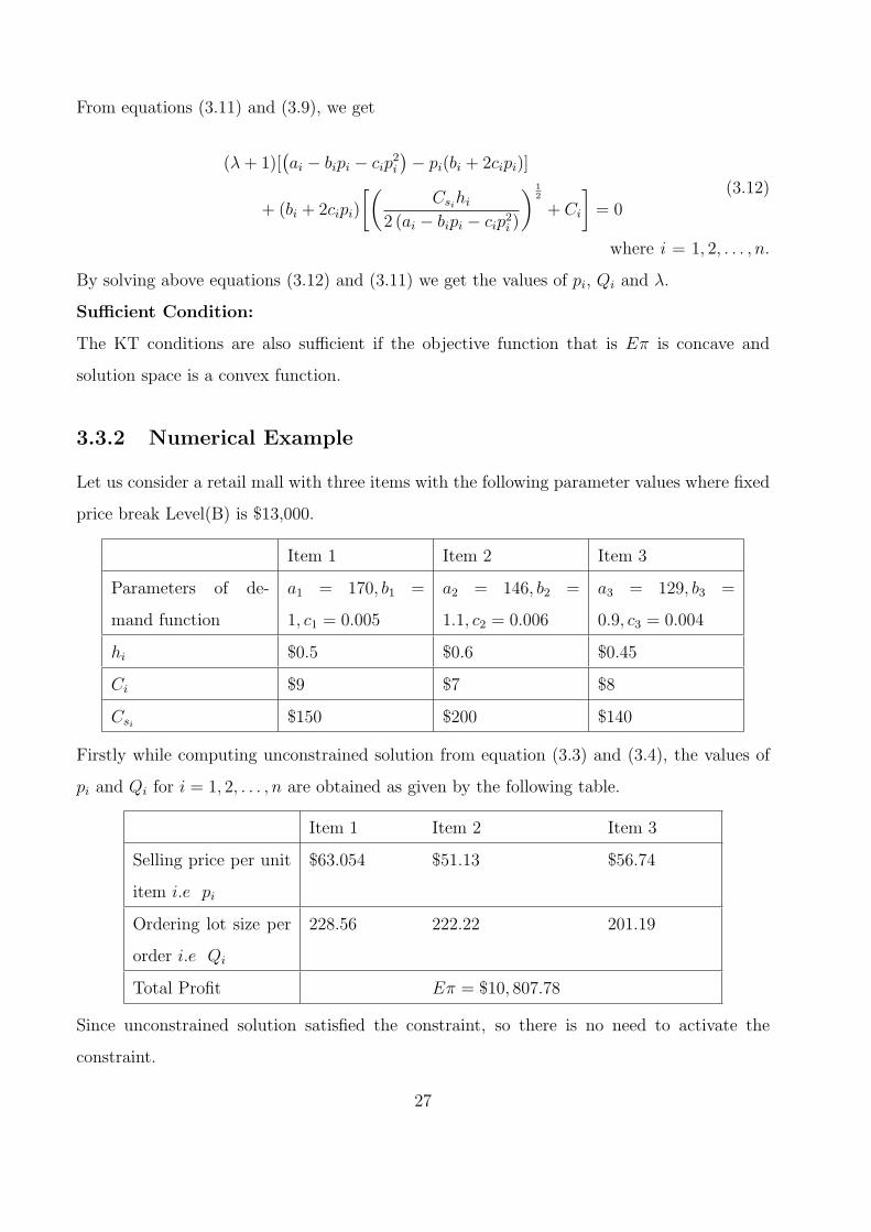
3.3.2 Numerical Example
Let us consider a retail mall with three items with the following parameter values where fixed
price break Level(B) is $13,000.
Item 1 Item 2 Item 3
Parameters of de-
mand function
a1 = 170, b1 =
1, c1 = 0.005
a2 = 146, b2 =
1.1, c2 = 0.006
a3 = 129, b3 =
0.9, c3 = 0.004
hi $0.5 $0.6 $0.45
Ci $9 $7 $8
Csi $150 $200 $140
Firstly while computing unconstrained solution from equation (3.3) and (3.4), the values of
pi and Qi for i = 1, 2, . . . , n are obtained as given by the following table.
Item 1 Item 2 Item 3
Selling price per unit
item i.e pi
$63.054 $51.13 $56.74
Ordering lot size per
order i.e Qi
228.56 222.22 201.19
Total Profit Eπ = $10, 807.78
Since unconstrained solution satisfied the constraint, so there is no need to activate the
constraint.
27
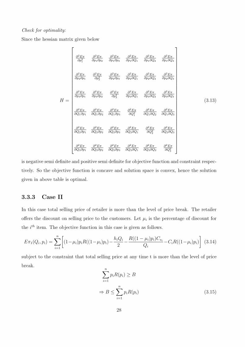
Check for optimality:
Since the hessian matrix given below
H =
∂2Eπ∂p21
∂2Eπ∂p1∂p2
∂2Eπ∂p1∂p3
∂2Eπ∂p1∂Q1
∂2Eπ∂p1∂Q2
∂2Eπ∂p1∂Q3
∂2Eπ∂p2∂p1
∂2Eπ∂p22
∂2Eπ∂p2∂p3
∂2Eπ∂p2∂Q1
∂2Eπ∂p2∂Q2
∂2Eπ∂p2∂Q3
∂2Eπ∂p3∂p1
∂2Eπ∂p3∂p2
∂2Eπ∂p23
∂2Eπ∂p3∂Q1
∂2Eπ∂p3∂Q2
∂2Eπ∂p3∂Q3
∂2Eπ∂Q1∂p1
∂2Eπ∂Q1∂p2
∂2Eπ∂Q1∂p3
∂2Eπ∂Q2
1
∂2Eπ∂Q1∂Q2
∂2Eπ∂Q1∂Q3
∂2Eπ∂Q2∂p1
∂2Eπ∂Q2∂p2
∂2Eπ∂Q2∂p3
∂2Eπ∂Q2∂Q1
∂2Eπ∂Q2
2
∂2Eπ∂Q2∂Q3
∂2Eπ∂Q3∂p1
∂2Eπ∂Q3∂p2
∂2Eπ∂Q3∂p3
∂2Eπ∂Q3∂Q1
∂2Eπ∂Q3∂Q2
∂2Eπ∂Q2
3
(3.13)
is negative semi definite and positive semi definite for objective function and constraint respec-
tively. So the objective function is concave and solution space is convex, hence the solution
given in above table is optimal.
3.3.3 Case II
In this case total selling price of retailer is more than the level of price break. The retailer
offers the discount on selling price to the customers. Let µi is the percentage of discount for
the ith item. The objective function in this case is given as follows.
Eπ1(Qi, pi) =n∑
i=1
[(1−µi)piR((1−µi)pi)−
hiQi
2−R((1− µi)pi)Csi
Qi
−CiR((1−µi)pi)
](3.14)
subject to the constraint that total selling price at any time t is more than the level of price
break.n∑
i=1
piR(pi) ≥ B
⇒ B ≤n∑
i=1
piR(pi) (3.15)
28
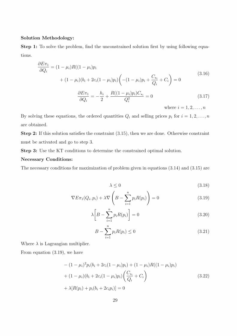
Solution Methodology:
Step 1: To solve the problem, find the unconstrained solution first by using following equa-
tions.
∂Eπ1
∂Qi
= (1− µi)R((1− µi)pi
+ (1− µi)(bi + 2ci(1− µi)pi)
(−(1− µi)pi +
Csi
Qi
+ Ci
)= 0
(3.16)
∂Eπ1
∂Qi
= −hi
2+
R((1− µi)pi)Csi
Q2i
= 0 (3.17)
where i = 1, 2, . . . , n
By solving these equations, the ordered quantities Qi and selling prices pi for i = 1, 2, . . . , n
are obtained.
Step 2: If this solution satisfies the constraint (3.15), then we are done. Otherwise constraint
must be activated and go to step 3.
Step 3: Use the KT conditions to determine the constrained optimal solution.
Necessary Conditions:
The necessary conditions for maximization of problem given in equations (3.14) and (3.15) are
λ ≤ 0 (3.18)
∇Eπ1(Qi, pi) + λ∇
(B −
n∑i=1
piR(pi)
)= 0 (3.19)
λ
[B −
n∑i=1
piR(pi)
]= 0 (3.20)
B −n∑
i=1
piR(pi) ≤ 0 (3.21)
Where λ is Lagrangian multiplier.
From equation (3.19), we have
− (1− µi)2pi(bi + 2ci(1− µi)pi) + (1− µi)R((1− µi)pi)
+ (1− µi)(bi + 2ci(1− µi)pi)
(Csi
Qi
+ Ci
)+ λ[R(pi) + pi(bi + 2cipi)] = 0
(3.22)
29
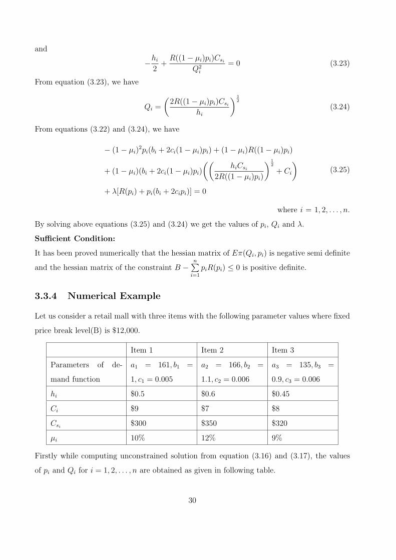
and
−hi
2+
R((1− µi)pi)Csi
Q2i
= 0 (3.23)
From equation (3.23), we have
Qi =
(2R((1− µi)pi)Csi
hi
) 12
(3.24)
From equations (3.22) and (3.24), we have
− (1− µi)2pi(bi + 2ci(1− µi)pi) + (1− µi)R((1− µi)pi)
+ (1− µi)(bi + 2ci(1− µi)pi)
((hiCsi
2R((1− µi)pi)
) 12
+ Ci
)+ λ[R(pi) + pi(bi + 2cipi)] = 0
(3.25)
where i = 1, 2, . . . , n.
By solving above equations (3.25) and (3.24) we get the values of pi, Qi and λ.
Sufficient Condition:
It has been proved numerically that the hessian matrix of Eπ(Qi, pi) is negative semi definite
and the hessian matrix of the constraint B −n∑
i=1
piR(pi) ≤ 0 is positive definite.
3.3.4 Numerical Example
Let us consider a retail mall with three items with the following parameter values where fixed
price break level(B) is $12,000.
Item 1 Item 2 Item 3
Parameters of de-
mand function
a1 = 161, b1 =
1, c1 = 0.005
a2 = 166, b2 =
1.1, c2 = 0.006
a3 = 135, b3 =
0.9, c3 = 0.006
hi $0.5 $0.6 $0.45
Ci $9 $7 $8
Csi $300 $350 $320
µi 10% 12% 9%
Firstly while computing unconstrained solution from equation (3.16) and (3.17), the values
of pi and Qi for i = 1, 2, . . . , n are obtained as given in following table.
30
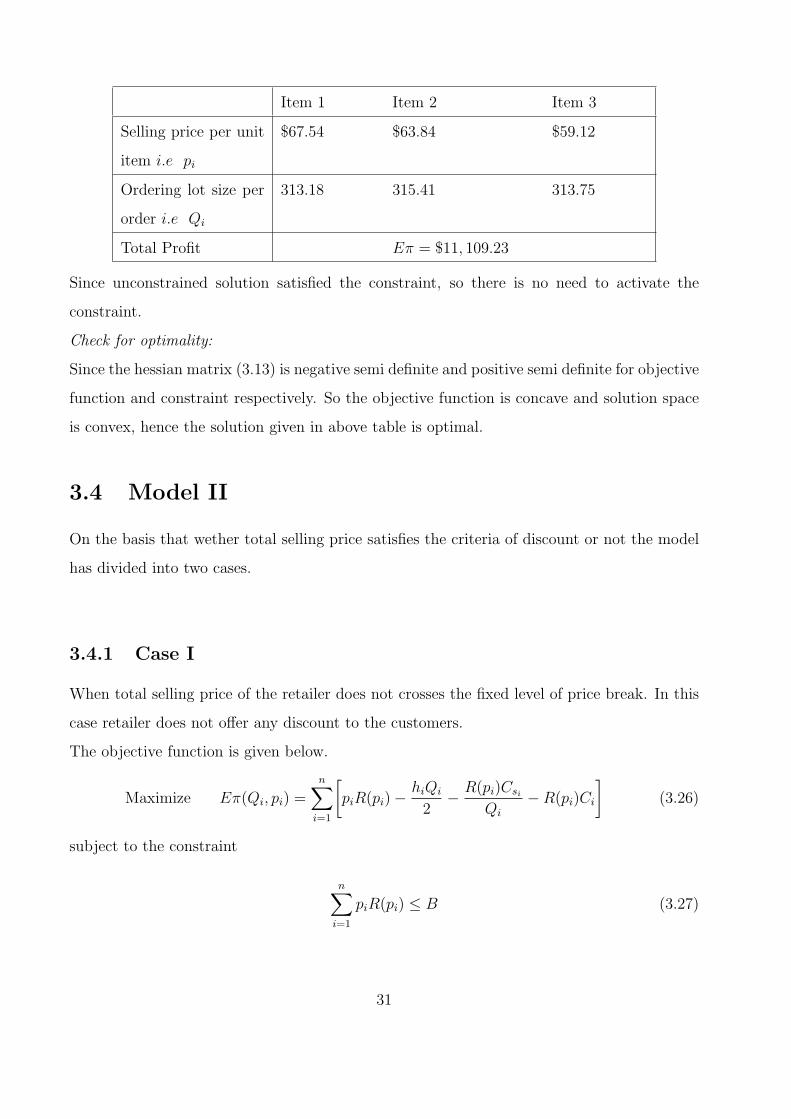
Item 1 Item 2 Item 3
Selling price per unit
item i.e pi
$67.54 $63.84 $59.12
Ordering lot size per
order i.e Qi
313.18 315.41 313.75
Total Profit Eπ = $11, 109.23
Since unconstrained solution satisfied the constraint, so there is no need to activate the
constraint.
Check for optimality:
Since the hessian matrix (3.13) is negative semi definite and positive semi definite for objective
function and constraint respectively. So the objective function is concave and solution space
is convex, hence the solution given in above table is optimal.
3.4 Model II
On the basis that wether total selling price satisfies the criteria of discount or not the model
has divided into two cases.
3.4.1 Case I
When total selling price of the retailer does not crosses the fixed level of price break. In this
case retailer does not offer any discount to the customers.
The objective function is given below.
Maximize Eπ(Qi, pi) =n∑
i=1
[piR(pi)−
hiQi
2− R(pi)Csi
Qi
−R(pi)Ci
](3.26)
subject to the constraint
n∑i=1
piR(pi) ≤ B (3.27)
31
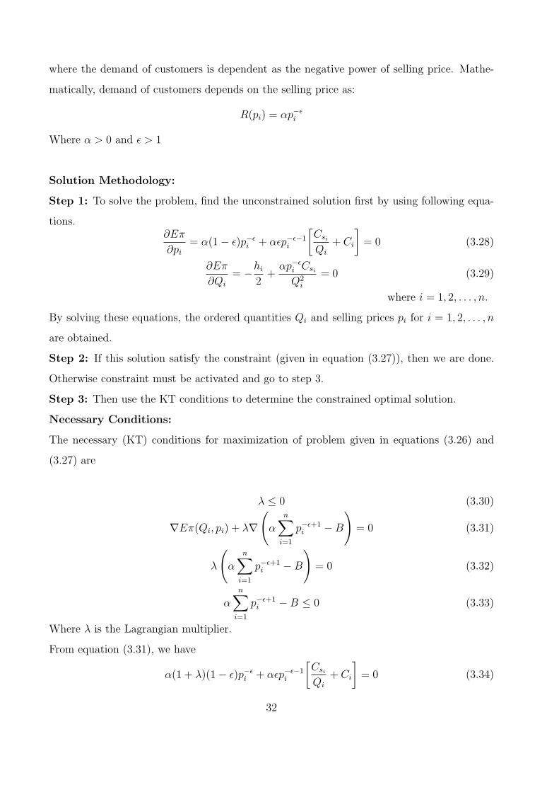
where the demand of customers is dependent as the negative power of selling price. Mathe-
matically, demand of customers depends on the selling price as:
R(pi) = αp−ϵi
Where α > 0 and ϵ > 1
Solution Methodology:
Step 1: To solve the problem, find the unconstrained solution first by using following equa-
tions.∂Eπ
∂pi= α(1− ϵ)p−ϵ
i + αϵp−ϵ−1i
[Csi
Qi
+ Ci
]= 0 (3.28)
∂Eπ
∂Qi
= −hi
2+
αp−ϵi Csi
Q2i
= 0 (3.29)
where i = 1, 2, . . . , n.
By solving these equations, the ordered quantities Qi and selling prices pi for i = 1, 2, . . . , n
are obtained.
Step 2: If this solution satisfy the constraint (given in equation (3.27)), then we are done.
Otherwise constraint must be activated and go to step 3.
Step 3: Then use the KT conditions to determine the constrained optimal solution.
Necessary Conditions:
The necessary (KT) conditions for maximization of problem given in equations (3.26) and
(3.27) are
λ ≤ 0 (3.30)
∇Eπ(Qi, pi) + λ∇
(α
n∑i=1
p−ϵ+1i −B
)= 0 (3.31)
λ
(α
n∑i=1
p−ϵ+1i −B
)= 0 (3.32)
α
n∑i=1
p−ϵ+1i −B ≤ 0 (3.33)
Where λ is the Lagrangian multiplier.
From equation (3.31), we have
α(1 + λ)(1− ϵ)p−ϵi + αϵp−ϵ−1
i
[Csi
Qi
+ Ci
]= 0 (3.34)
32
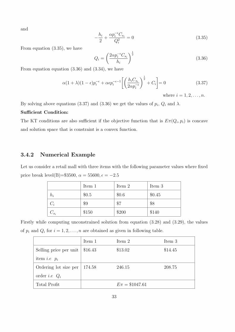
and
−hi
2+
αp−ϵi Csi
Q2i
= 0 (3.35)
From equation (3.35), we have
Qi =
(2αp−ϵ
i Csi
hi
) 12
(3.36)
From equation equation (3.36) and (3.34), we have
α(1 + λ)(1− ϵ)p−ϵi + αϵp−ϵ−1
i
[(hiCsi
2αp−ϵi
) 12
+ Ci
]= 0 (3.37)
where i = 1, 2, . . . , n.
By solving above equations (3.37) and (3.36) we get the values of pi, Qi and λ.
Sufficient Condition:
The KT conditions are also sufficient if the objective function that is Eπ(Qi, pi) is concave
and solution space that is constraint is a convex function.
3.4.2 Numerical Example
Let us consider a retail mall with three items with the following parameter values where fixed
price break level(B)=$3500, α = 55600, ϵ = −2.5
Item 1 Item 2 Item 3
hi $0.5 $0.6 $0.45
Ci $9 $7 $8
Csi $150 $200 $140
Firstly while computing unconstrained solution from equation (3.28) and (3.29), the values
of pi and Qi for i = 1, 2, . . . , n are obtained as given in following table.
Item 1 Item 2 Item 3
Selling price per unit
item i.e pi
$16.43 $13.02 $14.45
Ordering lot size per
order i.e Qi
174.58 246.15 208.75
Total Profit Eπ = $1047.61
33
Since unconstrained solution satisfied the constraint, so there is no need to activate the con-
straint.
Check for optimality:
Since the hessian matrix (3.13) is negative semi definite and positive semi definite for objec-
tive function and constraint respectively. So the objective function is concave and solution
space is convex, hence the solution given in above table is optimal.
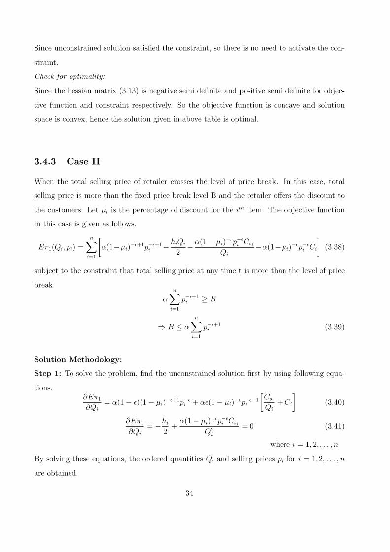
3.4.3 Case II
When the total selling price of retailer crosses the level of price break. In this case, total
selling price is more than the fixed price break level B and the retailer offers the discount to
the customers. Let µi is the percentage of discount for the ith item. The objective function
in this case is given as follows.
Eπ1(Qi, pi) =n∑
i=1
[α(1−µi)
−ϵ+1p−ϵ+1i − hiQi
2− α(1− µi)
−ϵp−ϵi Csi
Qi
−α(1−µi)−ϵp−ϵ
i Ci
](3.38)
subject to the constraint that total selling price at any time t is more than the level of price
break.
αn∑
i=1
p−ϵ+1i ≥ B
⇒ B ≤ αn∑
i=1
p−ϵ+1i (3.39)
Solution Methodology:
Step 1: To solve the problem, find the unconstrained solution first by using following equa-
tions.∂Eπ1
∂Qi
= α(1− ϵ)(1− µi)−ϵ+1p−ϵ
i + αϵ(1− µi)−ϵp−ϵ−1
i
[Csi
Qi
+ Ci
](3.40)
∂Eπ1
∂Qi
= −hi
2+
α(1− µi)−ϵp−ϵ
i Csi
Q2i
= 0 (3.41)
where i = 1, 2, . . . , n
By solving these equations, the ordered quantities Qi and selling prices pi for i = 1, 2, . . . , n
are obtained.
34
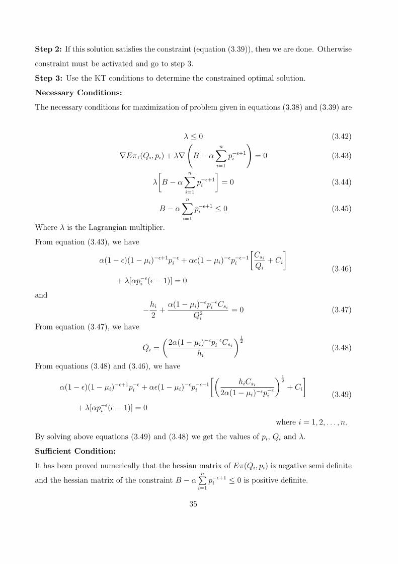
Step 2: If this solution satisfies the constraint (equation (3.39)), then we are done. Otherwise
constraint must be activated and go to step 3.
Step 3: Use the KT conditions to determine the constrained optimal solution.
Necessary Conditions:
The necessary conditions for maximization of problem given in equations (3.38) and (3.39) are
λ ≤ 0 (3.42)
∇Eπ1(Qi, pi) + λ∇
(B − α
n∑i=1
p−ϵ+1i
)= 0 (3.43)
λ
[B − α
n∑i=1
p−ϵ+1i
]= 0 (3.44)
B − α
n∑i=1
p−ϵ+1i ≤ 0 (3.45)
Where λ is the Lagrangian multiplier.
From equation (3.43), we have
α(1− ϵ)(1− µi)−ϵ+1p−ϵ
i + αϵ(1− µi)−ϵp−ϵ−1
i
[Csi
Qi
+ Ci
]+ λ[αp−ϵ
i (ϵ− 1)] = 0
(3.46)
and
−hi
2+
α(1− µi)−ϵp−ϵ
i Csi
Q2i
= 0 (3.47)
From equation (3.47), we have
Qi =
(2α(1− µi)
−ϵp−ϵi Csi
hi
) 12
(3.48)
From equations (3.48) and (3.46), we have
α(1− ϵ)(1− µi)−ϵ+1p−ϵ
i + αϵ(1− µi)−ϵp−ϵ−1
i
[(hiCsi
2α(1− µi)−ϵp−ϵi
) 12
+ Ci
]+ λ[αp−ϵ
i (ϵ− 1)] = 0
(3.49)
where i = 1, 2, . . . , n.
By solving above equations (3.49) and (3.48) we get the values of pi, Qi and λ.
Sufficient Condition:
It has been proved numerically that the hessian matrix of Eπ(Qi, pi) is negative semi definite
and the hessian matrix of the constraint B − αn∑
i=1
p−ϵ+1i ≤ 0 is positive definite.
35
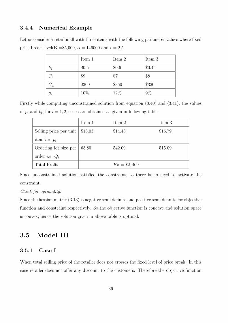
3.4.4 Numerical Example
Let us consider a retail mall with three items with the following parameter values where fixed
price break level(B)=$5,000, α = 146000 and ϵ = 2.5
Item 1 Item 2 Item 3
hi $0.5 $0.6 $0.45
Ci $9 $7 $8
Csi $300 $350 $320
µi 10% 12% 9%
Firstly while computing unconstrained solution from equation (3.40) and (3.41), the values
of pi and Qi for i = 1, 2, . . . , n are obtained as given in following table.
Item 1 Item 2 Item 3
Selling price per unit
item i.e pi
$18.03 $14.48 $15.79
Ordering lot size per
order i.e Qi
63.80 542.09 515.09
Total Profit Eπ = $2, 409
Since unconstrained solution satisfied the constraint, so there is no need to activate the
constraint.
Check for optimality:
Since the hessian matrix (3.13) is negative semi definite and positive semi definite for objective
function and constraint respectively. So the objective function is concave and solution space
is convex, hence the solution given in above table is optimal.
3.5 Model III
3.5.1 Case I
When total selling price of the retailer does not crosses the fixed level of price break. In this
case retailer does not offer any discount to the customers. Therefore the objective function
36
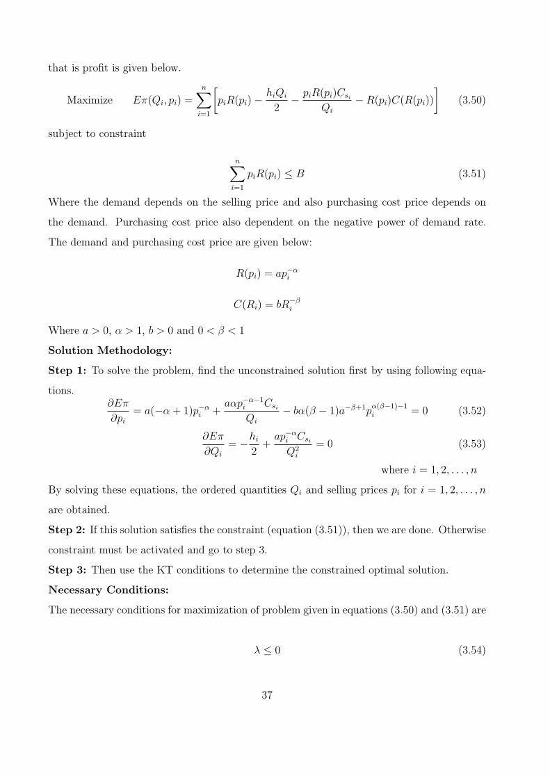
that is profit is given below.
Maximize Eπ(Qi, pi) =n∑
i=1
[piR(pi)−
hiQi
2− piR(pi)Csi
Qi
−R(pi)C(R(pi))
](3.50)
subject to constraint
n∑i=1
piR(pi) ≤ B (3.51)
Where the demand depends on the selling price and also purchasing cost price depends on
the demand. Purchasing cost price also dependent on the negative power of demand rate.
The demand and purchasing cost price are given below:
R(pi) = ap−αi
C(Ri) = bR−βi
Where a > 0, α > 1, b > 0 and 0 < β < 1
Solution Methodology:
Step 1: To solve the problem, find the unconstrained solution first by using following equa-
tions.∂Eπ
∂pi= a(−α+ 1)p−α
i +aαp−α−1
i Csi
Qi
− bα(β − 1)a−β+1pα(β−1)−1i = 0 (3.52)
∂Eπ
∂Qi
= −hi
2+
ap−αi Csi
Q2i
= 0 (3.53)
where i = 1, 2, . . . , n
By solving these equations, the ordered quantities Qi and selling prices pi for i = 1, 2, . . . , n
are obtained.
Step 2: If this solution satisfies the constraint (equation (3.51)), then we are done. Otherwise
constraint must be activated and go to step 3.
Step 3: Then use the KT conditions to determine the constrained optimal solution.
Necessary Conditions:
The necessary conditions for maximization of problem given in equations (3.50) and (3.51) are
λ ≤ 0 (3.54)
37
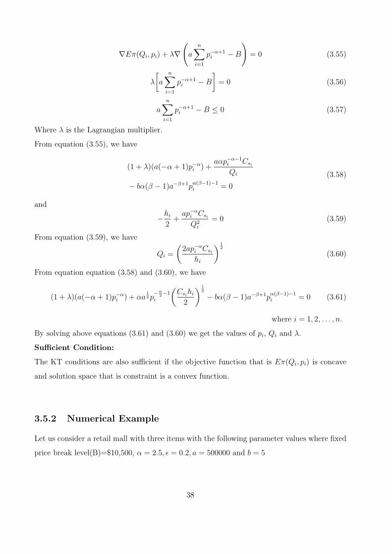
∇Eπ(Qi, pi) + λ∇
(a
n∑i=1
p−α+1i −B
)= 0 (3.55)
λ
[a
n∑i=1
p−α+1i −B
]= 0 (3.56)
an∑
i=1
p−α+1i −B ≤ 0 (3.57)
Where λ is the Lagrangian multiplier.
From equation (3.55), we have
(1 + λ)(a(−α+ 1)p−αi ) +
aαp−α−1i Csi
Qi
− bα(β − 1)a−β+1pα(β−1)−1i = 0
(3.58)
and
−hi
2+
ap−αi Csi
Q2i
= 0 (3.59)
From equation (3.59), we have
Qi =
(2ap−α
i Csi
hi
) 12
(3.60)
From equation equation (3.58) and (3.60), we have
(1 + λ)(a(−α+ 1)p−αi ) + αa
12p
−α2−1
i
(Csihi
2
) 12
− bα(β − 1)a−β+1pα(β−1)−1i = 0 (3.61)
where i = 1, 2, . . . , n.
By solving above equations (3.61) and (3.60) we get the values of pi, Qi and λ.
Sufficient Condition:
The KT conditions are also sufficient if the objective function that is Eπ(Qi, pi) is concave
and solution space that is constraint is a convex function.
3.5.2 Numerical Example
Let us consider a retail mall with three items with the following parameter values where fixed
price break level(B)=$10,500, α = 2.5, ϵ = 0.2, a = 500000 and b = 5
38
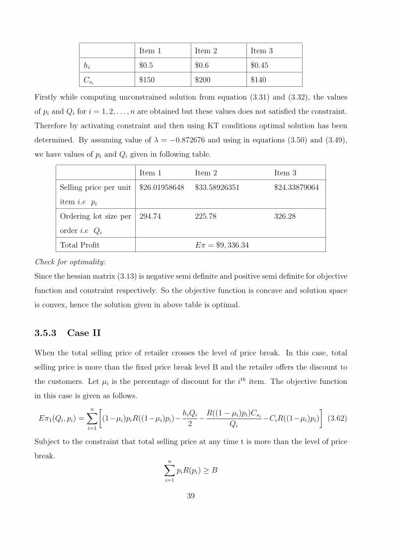
Item 1 Item 2 Item 3
hi $0.5 $0.6 $0.45
Csi $150 $200 $140
Firstly while computing unconstrained solution from equation (3.31) and (3.32), the values
of pi and Qi for i = 1, 2, . . . , n are obtained but these values does not satisfied the constraint.
Therefore by activating constraint and then using KT conditions optimal solution has been
determined. By assuming value of λ = −0.872676 and using in equations (3.50) and (3.49),
we have values of pi and Qi given in following table.
Item 1 Item 2 Item 3
Selling price per unit
item i.e pi
$26.01958648 $33.58926351 $24.33879064
Ordering lot size per
order i.e Qi
294.74 225.78 326.28
Total Profit Eπ = $9, 336.34
Check for optimality:
Since the hessian matrix (3.13) is negative semi definite and positive semi definite for objective
function and constraint respectively. So the objective function is concave and solution space
is convex, hence the solution given in above table is optimal.
3.5.3 Case II
When the total selling price of retailer crosses the level of price break. In this case, total
selling price is more than the fixed price break level B and the retailer offers the discount to
the customers. Let µi is the percentage of discount for the ith item. The objective function
in this case is given as follows.
Eπ1(Qi, pi) =n∑
i=1
[(1−µi)piR((1−µi)pi)−
hiQi
2−R((1− µi)pi)Csi
Qi
−CiR((1−µi)pi)
](3.62)
Subject to the constraint that total selling price at any time t is more than the level of price
break.n∑
i=1
piR(pi) ≥ B
39
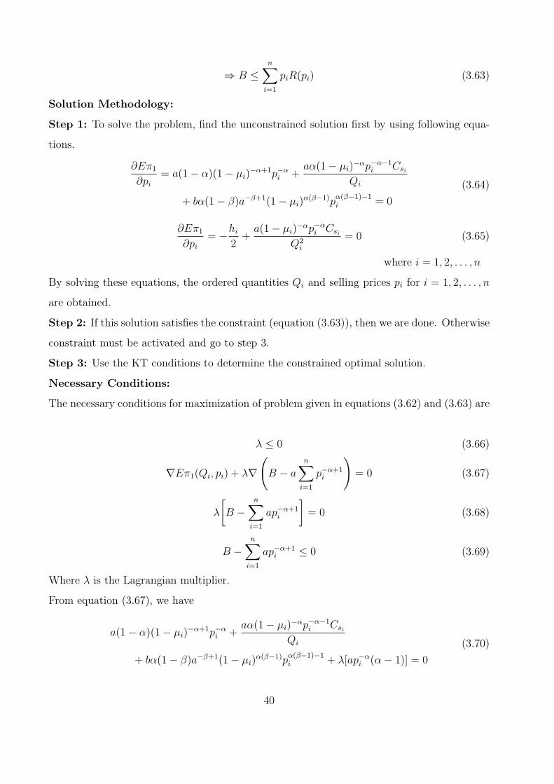
⇒ B ≤n∑
i=1
piR(pi) (3.63)
Solution Methodology:
Step 1: To solve the problem, find the unconstrained solution first by using following equa-
tions.
∂Eπ1
∂pi= a(1− α)(1− µi)
−α+1p−αi +
aα(1− µi)−αp−α−1
i Csi
Qi
+ bα(1− β)a−β+1(1− µi)α(β−1)p
α(β−1)−1i = 0
(3.64)
∂Eπ1
∂pi= −hi
2+
a(1− µi)−αp−α
i Csi
Q2i
= 0 (3.65)
where i = 1, 2, . . . , n
By solving these equations, the ordered quantities Qi and selling prices pi for i = 1, 2, . . . , n
are obtained.
Step 2: If this solution satisfies the constraint (equation (3.63)), then we are done. Otherwise
constraint must be activated and go to step 3.
Step 3: Use the KT conditions to determine the constrained optimal solution.
Necessary Conditions:
The necessary conditions for maximization of problem given in equations (3.62) and (3.63) are
λ ≤ 0 (3.66)
∇Eπ1(Qi, pi) + λ∇
(B − a
n∑i=1
p−α+1i
)= 0 (3.67)
λ
[B −
n∑i=1
ap−α+1i
]= 0 (3.68)
B −n∑
i=1
ap−α+1i ≤ 0 (3.69)
Where λ is the Lagrangian multiplier.
From equation (3.67), we have
a(1− α)(1− µi)−α+1p−α
i +aα(1− µi)
−αp−α−1i Csi
Qi
+ bα(1− β)a−β+1(1− µi)α(β−1)p
α(β−1)−1i + λ[ap−α
i (α− 1)] = 0
(3.70)
40
and
−hi
2+
a(1− µi)−αp−α
i Csi
Q2i
= 0 (3.71)
From equation (3.71), we have
Qi =
(2a(1− µi)
−αp−αi Csi
hi
) 12
(3.72)
From equations (3.72) and (3.70), we get
a(1− α)(1− µi)−α+1p−α
i + αa12 (1− µi)
− 12p
−α2−1
i
(Csihi
2
) 12
+ bα(1− β)a−β+1(1− µi)α(β−1)p
α(β−1)−1i + λ[ap−α
i (α− 1)] = 0
(3.73)
where i = 1, 2, . . . , n.
By solving above equations (3.73) and (3.72) we get the values of pi, Qi and λ.
Sufficient Condition:
It has been proved numerically that the hessian matrix of Eπ(Qi, pi) is negative semi definite
and the hessian matrix of the constraint B − αn∑
i=1
p−ϵ+1i ≤ 0 is positive definite.
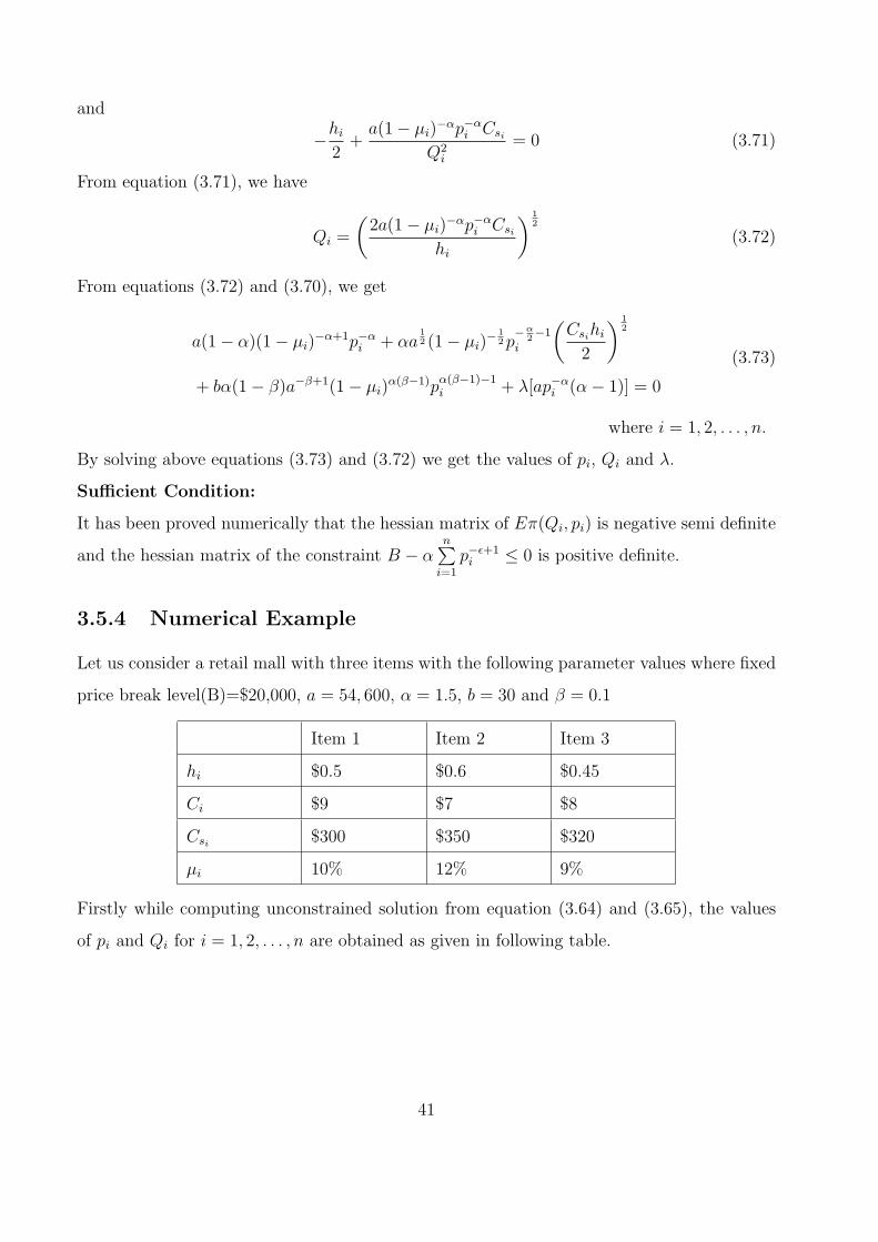
3.5.4 Numerical Example
Let us consider a retail mall with three items with the following parameter values where fixed
price break level(B)=$20,000, a = 54, 600, α = 1.5, b = 30 and β = 0.1
Item 1 Item 2 Item 3
hi $0.5 $0.6 $0.45
Ci $9 $7 $8
Csi $300 $350 $320
µi 10% 12% 9%
Firstly while computing unconstrained solution from equation (3.64) and (3.65), the values
of pi and Qi for i = 1, 2, . . . , n are obtained as given in following table.
41
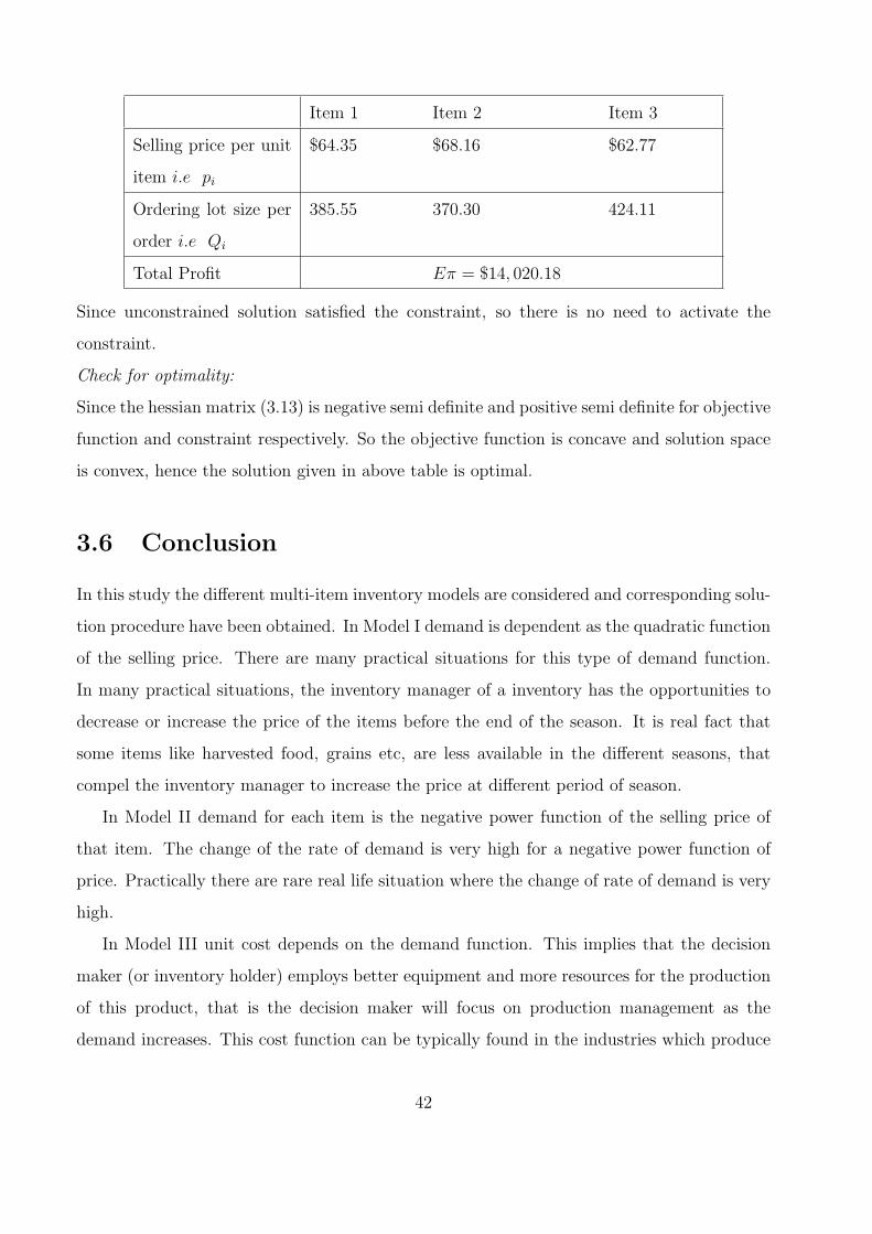
Item 1 Item 2 Item 3
Selling price per unit
item i.e pi
$64.35 $68.16 $62.77
Ordering lot size per
order i.e Qi
385.55 370.30 424.11
Total Profit Eπ = $14, 020.18
Since unconstrained solution satisfied the constraint, so there is no need to activate the
constraint.
Check for optimality:
Since the hessian matrix (3.13) is negative semi definite and positive semi definite for objective
function and constraint respectively. So the objective function is concave and solution space
is convex, hence the solution given in above table is optimal.
3.6 Conclusion
In this study the different multi-item inventory models are considered and corresponding solu-
tion procedure have been obtained. In Model I demand is dependent as the quadratic function
of the selling price. There are many practical situations for this type of demand function.
In many practical situations, the inventory manager of a inventory has the opportunities to
decrease or increase the price of the items before the end of the season. It is real fact that
some items like harvested food, grains etc, are less available in the different seasons, that
compel the inventory manager to increase the price at different period of season.
In Model II demand for each item is the negative power function of the selling price of
that item. The change of the rate of demand is very high for a negative power function of
price. Practically there are rare real life situation where the change of rate of demand is very
high.
In Model III unit cost depends on the demand function. This implies that the decision
maker (or inventory holder) employs better equipment and more resources for the production
of this product, that is the decision maker will focus on production management as the
demand increases. This cost function can be typically found in the industries which produce
42
a successful technologically advanced products such as computer industry. Therefore the
decision maker will justify the more efficient production processes as the demand increases.
43
Chapter 4
Multi-item Inventory Model in which
Demand Depends on Selling Price
under Storage, Investment and
Average Inventory Level Constraint.
4.1 Introduction
In this chapter, three multi-item inventory models have been considered. In these models the
objective function is the total profit obtained from an inventory has been considered same for
all three models and is similar to the objective function considered in chapter 3, the demand is
quadratically dependent on selling price for all models. The objective function is maximized
under storage, investment and average inventory level constraint separately. In all the three
models KT conditions are used to find the optimal solutions.
In first model total profit is subject to the limited storage space for all items in the
inventory that is total area required by all the items should be less than the available storage
area.
In second model total profit is subject to the limited investment available. In this model
inventory holder places a limit on the amount of investment to be carried that is the total
purchasing cost should be less than or equals to the available investment.
44
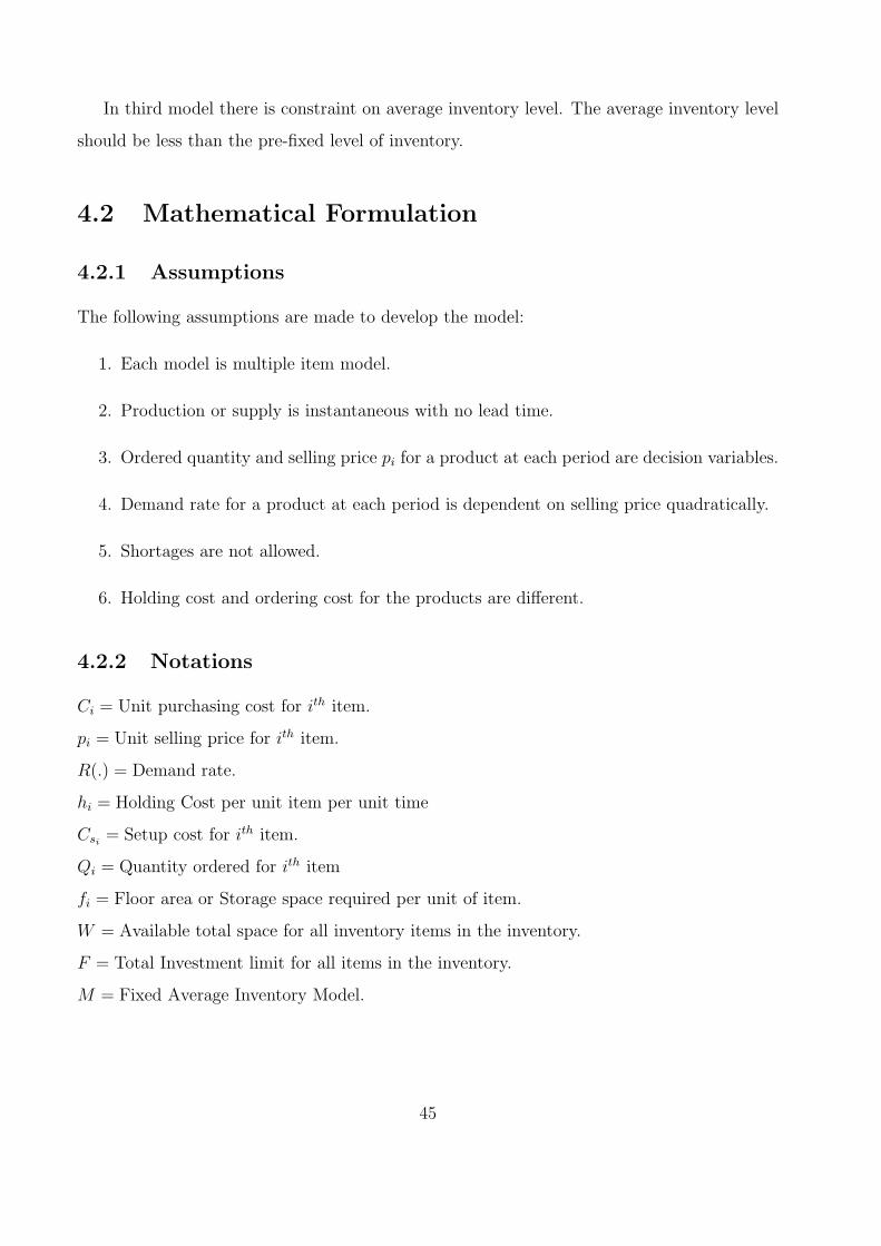
In third model there is constraint on average inventory level. The average inventory level
should be less than the pre-fixed level of inventory.
4.2 Mathematical Formulation
4.2.1 Assumptions
The following assumptions are made to develop the model:
1. Each model is multiple item model.
2. Production or supply is instantaneous with no lead time.
3. Ordered quantity and selling price pi for a product at each period are decision variables.
4. Demand rate for a product at each period is dependent on selling price quadratically.
5. Shortages are not allowed.
6. Holding cost and ordering cost for the products are different.
4.2.2 Notations
Ci = Unit purchasing cost for ith item.
pi = Unit selling price for ith item.
R(.) = Demand rate.
hi = Holding Cost per unit item per unit time
Csi = Setup cost for ith item.
Qi = Quantity ordered for ith item
fi = Floor area or Storage space required per unit of item.
W = Available total space for all inventory items in the inventory.
F = Total Investment limit for all items in the inventory.
M = Fixed Average Inventory Model.
45
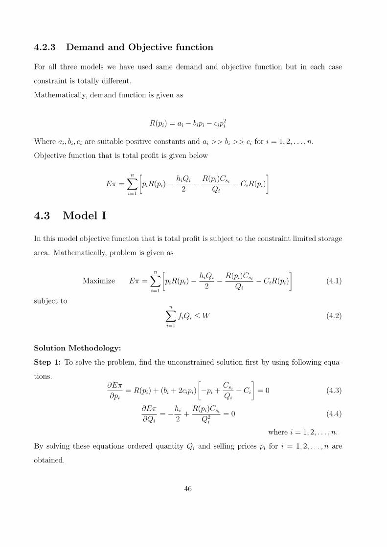
4.2.3 Demand and Objective function
For all three models we have used same demand and objective function but in each case
constraint is totally different.
Mathematically, demand function is given as
R(pi) = ai − bipi − cip2i
Where ai, bi, ci are suitable positive constants and ai >> bi >> ci for i = 1, 2, . . . , n.
Objective function that is total profit is given below
Eπ =n∑
i=1
[piR(pi)−
hiQi
2− R(pi)Csi
Qi
− CiR(pi)
]
4.3 Model I
In this model objective function that is total profit is subject to the constraint limited storage
area. Mathematically, problem is given as
Maximize Eπ =n∑
i=1
[piR(pi)−
hiQi
2− R(pi)Csi
Qi
− CiR(pi)
](4.1)
subject ton∑
i=1
fiQi ≤ W (4.2)
Solution Methodology:
Step 1: To solve the problem, find the unconstrained solution first by using following equa-
tions.∂Eπ
∂pi= R(pi) + (bi + 2cipi)
[−pi +
Csi
Qi
+ Ci
]= 0 (4.3)
∂Eπ
∂Qi
= −hi
2+
R(pi)Csi
Q2i
= 0 (4.4)
where i = 1, 2, . . . , n.
By solving these equations ordered quantity Qi and selling prices pi for i = 1, 2, . . . , n are
obtained.
46
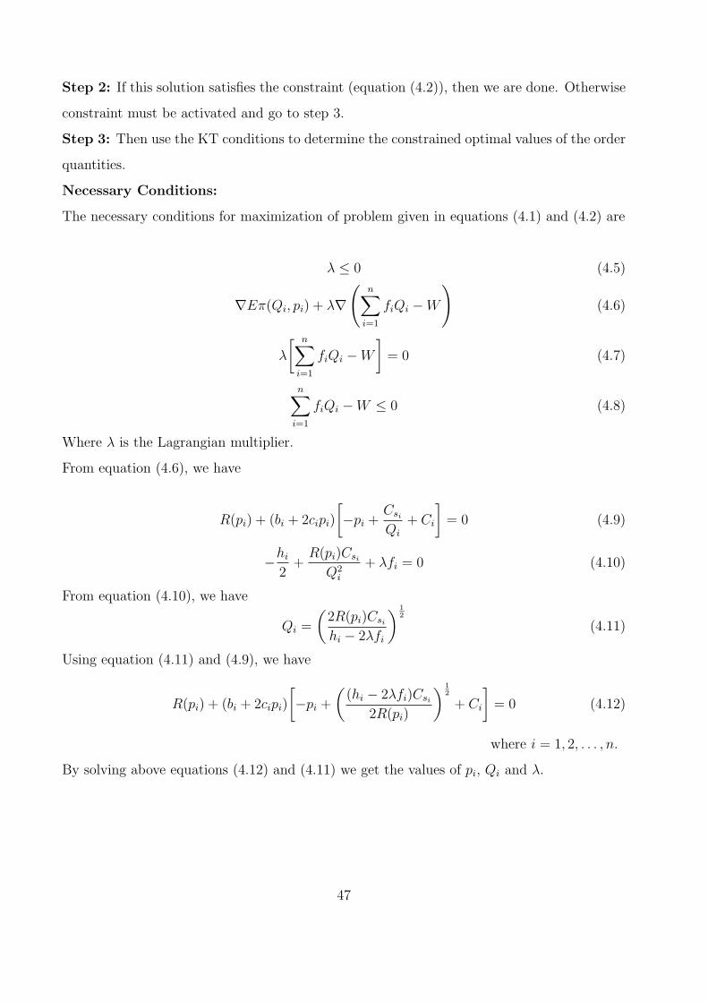
Step 2: If this solution satisfies the constraint (equation (4.2)), then we are done. Otherwise
constraint must be activated and go to step 3.
Step 3: Then use the KT conditions to determine the constrained optimal values of the order
quantities.
Necessary Conditions:
The necessary conditions for maximization of problem given in equations (4.1) and (4.2) are
λ ≤ 0 (4.5)
∇Eπ(Qi, pi) + λ∇
(n∑
i=1
fiQi −W
)(4.6)
λ
[ n∑i=1
fiQi −W
]= 0 (4.7)
n∑i=1
fiQi −W ≤ 0 (4.8)
Where λ is the Lagrangian multiplier.
From equation (4.6), we have
R(pi) + (bi + 2cipi)
[−pi +
Csi
Qi
+ Ci
]= 0 (4.9)
−hi
2+
R(pi)Csi
Q2i
+ λfi = 0 (4.10)
From equation (4.10), we have
Qi =
(2R(pi)Csi
hi − 2λfi
) 12
(4.11)
Using equation (4.11) and (4.9), we have
R(pi) + (bi + 2cipi)
[−pi +
((hi − 2λfi)Csi
2R(pi)
) 12
+ Ci
]= 0 (4.12)
where i = 1, 2, . . . , n.
By solving above equations (4.12) and (4.11) we get the values of pi, Qi and λ.
47
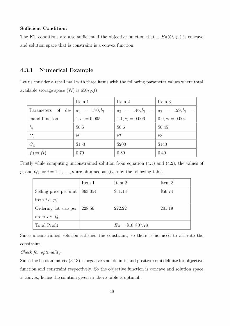
Sufficient Condition:
The KT conditions are also sufficient if the objective function that is Eπ(Qi, pi) is concave
and solution space that is constraint is a convex function.
4.3.1 Numerical Example
Let us consider a retail mall with three items with the following parameter values where total
available storage space (W) is 650sq.ft
Item 1 Item 2 Item 3
Parameters of de-
mand function
a1 = 170, b1 =
1, c1 = 0.005
a2 = 146, b2 =
1.1, c2 = 0.006
a3 = 129, b3 =
0.9, c3 = 0.004
hi $0.5 $0.6 $0.45
Ci $9 $7 $8
Csi $150 $200 $140
fi(sq.ft) 0.70 0.80 0.40
Firstly while computing unconstrained solution from equation (4.1) and (4.2), the values of
pi and Qi for i = 1, 2, . . . , n are obtained as given by the following table.
Item 1 Item 2 Item 3
Selling price per unit
item i.e pi
$63.054 $51.13 $56.74
Ordering lot size per
order i.e Qi
228.56 222.22 201.19
Total Profit Eπ = $10, 807.78
Since unconstrained solution satisfied the constraint, so there is no need to activate the
constraint.
Check for optimality:
Since the hessian matrix (3.13) is negative semi definite and positive semi definite for objective
function and constraint respectively. So the objective function is concave and solution space
is convex, hence the solution given in above table is optimal.
48
4.4 Model II
In this model objective function that is total profit is subject to the constraint limited invest-
ment available. Mathematically problem is
Maximize Eπ =n∑
i=1
[piR(pi)−
hiQi
2− R(pi)Csi
Qi
− CiR(pi)
](4.13)
subject ton∑
i=1
CiQi ≤ F (4.14)
Solution Methodology:
Step 1: To solve the problem, find the unconstrained solution first by using following equa-
tions.∂Eπ
∂pi= R(pi) + (bi + 2cipi)
[−pi +
Csi
Qi
+ Ci
]= 0 (4.15)
∂Eπ
∂Qi
= −hi
2+
R(pi)Csi
Q2i
= 0 (4.16)
where i = 1, 2, . . . , n.
By solving these equations ordered quantity Qi and selling prices pi for i = 1, 2, . . . , n. are
obtained.
Step 2: If this solution satisfies the constraint (equation (4.2)), then we are done. Otherwise
constraint must be activated and go to step 3.
Step 3: Then use the KT conditions to determine the constrained optimal values of the order
quantities.
Necessary Conditions:
The necessary conditions for maximization of problem given in equations (4.13) and (4.14) are
λ ≤ 0 (4.17)
∇Eπ(Qi, pi) + λ∇
(n∑
i=1
QiCi − F
)= 0 (4.18)
λ
[ n∑i=1
CiQi − F
]= 0 (4.19)
n∑i=1
CiQi − F ≤ 0 (4.20)
49
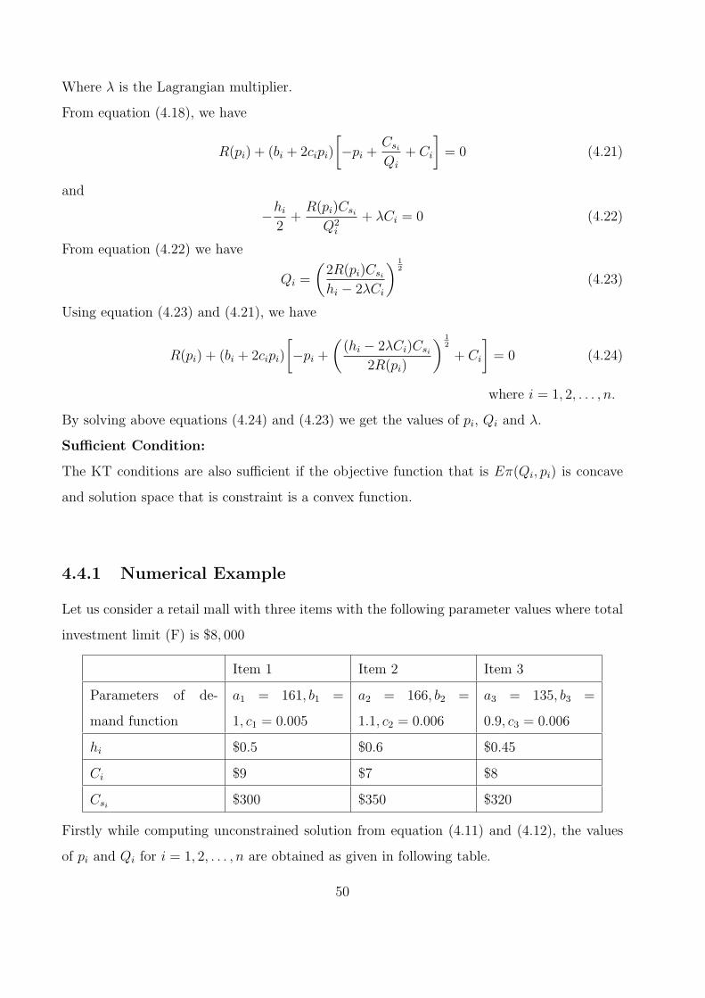
Where λ is the Lagrangian multiplier.
From equation (4.18), we have
R(pi) + (bi + 2cipi)
[−pi +
Csi
Qi
+ Ci
]= 0 (4.21)
and
−hi
2+
R(pi)Csi
Q2i
+ λCi = 0 (4.22)
From equation (4.22) we have
Qi =
(2R(pi)Csi
hi − 2λCi
) 12
(4.23)
Using equation (4.23) and (4.21), we have
R(pi) + (bi + 2cipi)
[−pi +
((hi − 2λCi)Csi
2R(pi)
) 12
+ Ci
]= 0 (4.24)
where i = 1, 2, . . . , n.
By solving above equations (4.24) and (4.23) we get the values of pi, Qi and λ.
Sufficient Condition:
The KT conditions are also sufficient if the objective function that is Eπ(Qi, pi) is concave
and solution space that is constraint is a convex function.
4.4.1 Numerical Example
Let us consider a retail mall with three items with the following parameter values where total
investment limit (F) is $8, 000
Item 1 Item 2 Item 3
Parameters of de-
mand function
a1 = 161, b1 =
1, c1 = 0.005
a2 = 166, b2 =
1.1, c2 = 0.006
a3 = 135, b3 =
0.9, c3 = 0.006
hi $0.5 $0.6 $0.45
Ci $9 $7 $8
Csi $300 $350 $320
Firstly while computing unconstrained solution from equation (4.11) and (4.12), the values
of pi and Qi for i = 1, 2, . . . , n are obtained as given in following table.
50
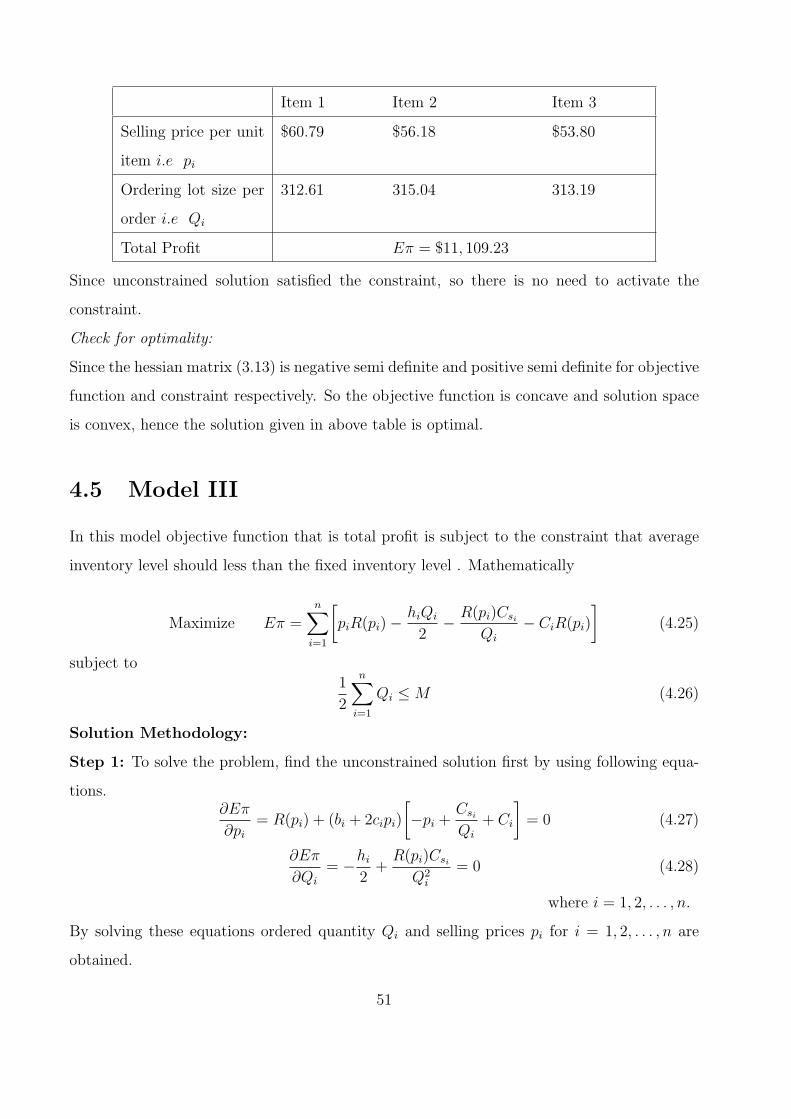
Item 1 Item 2 Item 3
Selling price per unit
item i.e pi
$60.79 $56.18 $53.80
Ordering lot size per
order i.e Qi
312.61 315.04 313.19
Total Profit Eπ = $11, 109.23
Since unconstrained solution satisfied the constraint, so there is no need to activate the
constraint.
Check for optimality:
Since the hessian matrix (3.13) is negative semi definite and positive semi definite for objective
function and constraint respectively. So the objective function is concave and solution space
is convex, hence the solution given in above table is optimal.
4.5 Model III
In this model objective function that is total profit is subject to the constraint that average
inventory level should less than the fixed inventory level . Mathematically
Maximize Eπ =n∑
i=1
[piR(pi)−
hiQi
2− R(pi)Csi
Qi
− CiR(pi)
](4.25)
subject to1
2
n∑i=1
Qi ≤ M (4.26)
Solution Methodology:
Step 1: To solve the problem, find the unconstrained solution first by using following equa-
tions.∂Eπ
∂pi= R(pi) + (bi + 2cipi)
[−pi +
Csi
Qi
+ Ci
]= 0 (4.27)
∂Eπ
∂Qi
= −hi
2+
R(pi)Csi
Q2i
= 0 (4.28)
where i = 1, 2, . . . , n.
By solving these equations ordered quantity Qi and selling prices pi for i = 1, 2, . . . , n are
obtained.
51
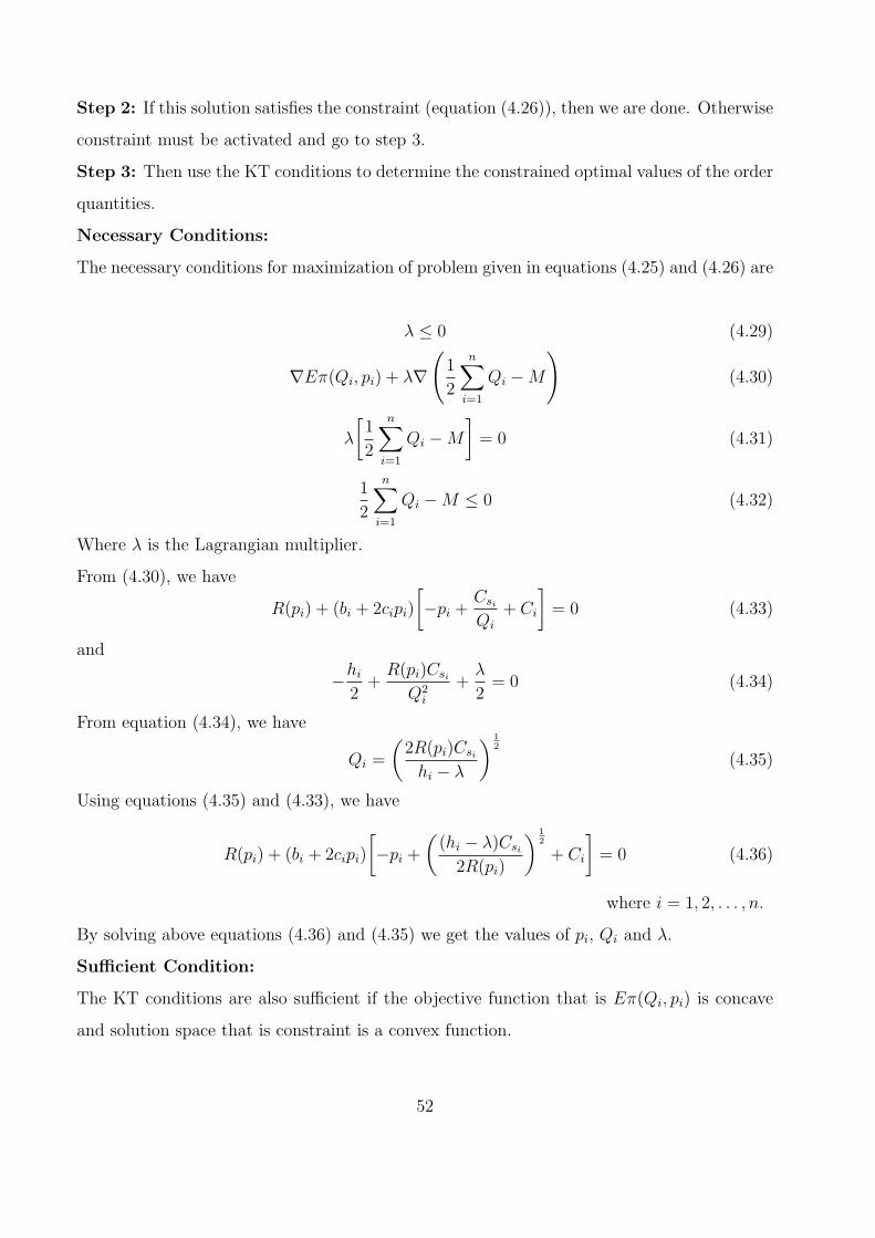
Step 2: If this solution satisfies the constraint (equation (4.26)), then we are done. Otherwise
constraint must be activated and go to step 3.
Step 3: Then use the KT conditions to determine the constrained optimal values of the order
quantities.
Necessary Conditions:
The necessary conditions for maximization of problem given in equations (4.25) and (4.26) are
λ ≤ 0 (4.29)
∇Eπ(Qi, pi) + λ∇
(1
2
n∑i=1
Qi −M
)(4.30)
λ
[1
2
n∑i=1
Qi −M
]= 0 (4.31)
1
2
n∑i=1
Qi −M ≤ 0 (4.32)
Where λ is the Lagrangian multiplier.
From (4.30), we have
R(pi) + (bi + 2cipi)
[−pi +
Csi
Qi
+ Ci
]= 0 (4.33)
and
−hi
2+
R(pi)Csi
Q2i
+λ
2= 0 (4.34)
From equation (4.34), we have
Qi =
(2R(pi)Csi
hi − λ
) 12
(4.35)
Using equations (4.35) and (4.33), we have
R(pi) + (bi + 2cipi)
[−pi +
((hi − λ)Csi
2R(pi)
) 12
+ Ci
]= 0 (4.36)
where i = 1, 2, . . . , n.
By solving above equations (4.36) and (4.35) we get the values of pi, Qi and λ.
Sufficient Condition:
The KT conditions are also sufficient if the objective function that is Eπ(Qi, pi) is concave
and solution space that is constraint is a convex function.
52
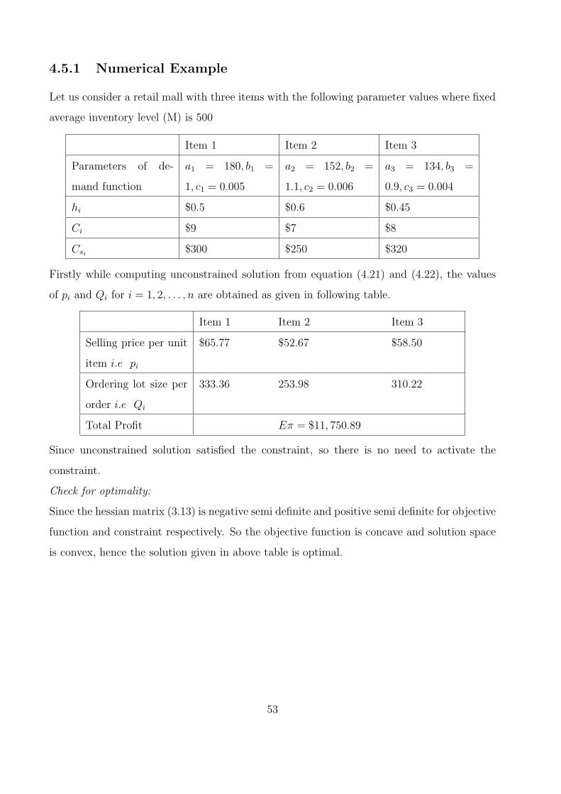
4.5.1 Numerical Example
Let us consider a retail mall with three items with the following parameter values where fixed
average inventory level (M) is 500
Item 1 Item 2 Item 3
Parameters of de-
mand function
a1 = 180, b1 =
1, c1 = 0.005
a2 = 152, b2 =
1.1, c2 = 0.006
a3 = 134, b3 =
0.9, c3 = 0.004
hi $0.5 $0.6 $0.45
Ci $9 $7 $8
Csi $300 $250 $320
Firstly while computing unconstrained solution from equation (4.21) and (4.22), the values
of pi and Qi for i = 1, 2, . . . , n are obtained as given in following table.
Item 1 Item 2 Item 3
Selling price per unit
item i.e pi
$65.77 $52.67 $58.50
Ordering lot size per
order i.e Qi
333.36 253.98 310.22
Total Profit Eπ = $11, 750.89
Since unconstrained solution satisfied the constraint, so there is no need to activate the
constraint.
Check for optimality:
Since the hessian matrix (3.13) is negative semi definite and positive semi definite for objective
function and constraint respectively. So the objective function is concave and solution space
is convex, hence the solution given in above table is optimal.
53
4.6 Conclusion
In this chapter, three multi-item inventory models have been studied, the objective function
has been considered as the total profit obtained from an inventory same for all three models.
The demand is quadratically dependent on selling price for all models. The objective function
is maximized under storage, investment and average inventory level constraint separately.
The solution procedure is developed using KT conditions. In the practical situation, there
are various types of competitions among the retailers or inventory holders who are holding
same type of inventory items. Also they have to face several problem like limited space in
warehouse(or inventory storage), investment limitations and inventory level limitation etc.
54
References
[1] H.A. Taha, Operation Research An Introduction, Prentice Hall of India, Sixth
edition, 2001.
[2] J.K. Sharma, Operations Research Theory and Applications, Macmillan India
Press, Third edition, 2007.
[3] B.Pal,S.S.Sana and K.Chaudhuri, Multi-item EOQ model while demand is sales
price and price break sensitive, Economic Modeling, 29, 2283− 2288(2012).
[4] S.S.Sana, Price-sensitive demand for perishable items-an EOQ model, Applied
Mathematics and Computation, 217, 6248− 6259(2011).
[5] H.Jung and C.M. Klein, Optimal inventory policies for profit maximizing EOQ
models under various cost functions, Europeon Journal of Operation Research,
174, 684− 705(2006).
[6] L.E.C.Barron and S.S.Sana, Multi-item EOQ model in a two-layer supply chain
while demand varies with promotional effort, Applied Mathematical Modelling,
xx,xxx-xxx(2015) .
[7] B.Pal, S.S.Sana and K.Chaudhri, A three layer multi-item production inven-
tory model for multiple suppliers and retailers, Economic Modelling, 29, 2704−
2710(2012).
[8] P.Guchhait, M.K.Maiti, Multi-item inventory model of breakable items with
stock dependent demand under stock and time dependent breakability rate,
Computers and Industrial Engineering, 59, 911− 920(2010).
55
[9] D.K.Bhattacharya, On multi-item inventory, European Journal of Operation
Research, 162, 786− 791(2005).
[10] G.Zhang, The multi-product newsboy problem with supplier quantity discounts
and a budget constraint, European Journal of Operation Research, 206, 350−
360(2010).
[11] S.S.Sana, Demand influenced by enterprises initiatives- A multi-item EOQ
model of deteriorating and ameliorating items, Mathematical and Computer
Modelling, 52, 284− 302(2010).
[12] C.Haksever and J.Mossourakis, A model for optimizing multi-product inven-
tory systems with multiple constraints, International Journal of Production
Economics. 97, 18− 30(2005).
[13] S.C.Graves, Note on the deterministic demand multi-product single-machine
lot scheduling problem, Management Sciences, 25(3), 276− 280(1979).
[14] K.A.M.Kotb, H.A.Fergany, Multi-item EOQ model with both demand depen-
dent unit cost and varying lead time via geometric programming, Applied
Mathematics, 2, 551− 555(2011).
[15] R.P.Tripathi and S.M.Mishra, Inventory model with inventory dependent de-
mand for deteriorating items in a single warehouse system, Uncertain Supply
Chain Management, 2, 209− 218(2014).
[16] P.Brandimarte, Multi-item capacitated lot sizing with demand uncertainty, In-
ternational Journal of Production Research, 44 : 15, 2997− 3002(2006), .
[17] S.Minner, Multiple-supplier inventory models in supply chain management: A
review, International Journal of Production Economics, 81−82, 265−279(2003).
[18] S.S.Sana, Optimal selling price and lotsize with time varying deterioration
and partial backlogging, Applied Mathematics and Computation, 217, 185 −
194(2010).
56
[19] H.M.Wee, W.T.Wang and C.J.Chung, A modified method to compute economic
order quantities with derivatives by cost-difference comparisons,European Jour-
nal of Operation Research, 194, 336− 338(2009).
[20] S.M.Samak and N.R.Rajhans, Determination of optimum inventory model for
minimizing total inventory cost, Production Engineering, 51, 803− 809(2013).
[21] K.Skouri and S.Papachristos, A continuous review inventory model with deteri-
orating items, time varying demand, linear replenishment cost, partially time-
varying backlogging, Applied Mathematical Modelling, 26, 603− 617(2002).
[22] S.P.Wang , An inventory replenishment policy for deteriorating items with
shortages and partial backlogging, Computers and Operation Research,
29, 2043− 2051(2002).
[23] D.W.Pentico and M.J.Drake, The deterministic EOQ with partial backorder-
ing: A new approach, European Journal of Operation Research, 194, 102 −
113(2009).
[24] R.Kian, U.Gurler and E.Berk, The dynamic lot-sizing problem with convex
economic production cost and setups, International Journal of Production Eco-
nomics, 155, 361− 379(2014).
[25] J.D.Lenard and B.Roy, Multi-item inventory control: A multicriteria view,
European Journal of Operation Research, 87, 685− 692(1995).
57