Multiple-imputation analysis using Stata's mi command · mi estimateperforms individual completed-data analyses (step 2), and then uses Rubin’s combination rules to consolidate

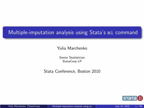
Multiple-imputation analysis using Stata’s mi command

Yulia Marchenko

Senior StatisticianStataCorp LP

Stata Conference, Boston 2010

Yulia Marchenko (StataCorp) Multiple-imputation analysis using mi July 16, 2010 1 / 50

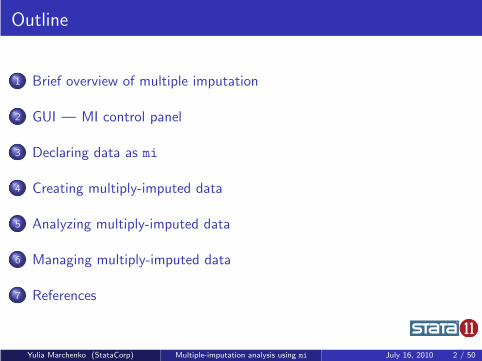
Outline

1 Brief overview of multiple imputation

2 GUI — MI control panel

3 Declaring data as mi

4 Creating multiply-imputed data

5 Analyzing multiply-imputed data

6 Managing multiply-imputed data

7 References


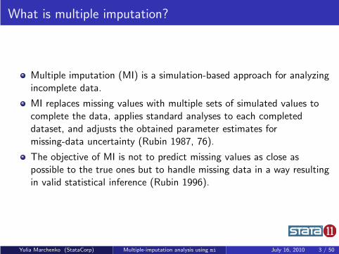
What is multiple imputation?

Multiple imputation (MI) is a simulation-based approach for analyzingincomplete data.

MI replaces missing values with multiple sets of simulated values tocomplete the data, applies standard analyses to each completeddataset, and adjusts the obtained parameter estimates formissing-data uncertainty (Rubin 1987, 76).

The objective of MI is not to predict missing values as close aspossible to the true ones but to handle missing data in a way resultingin valid statistical inference (Rubin 1996).


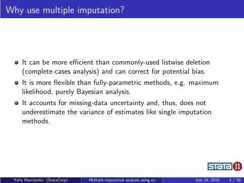
Why use multiple imputation?

It can be more efficient than commonly-used listwise deletion(complete-cases analysis) and can correct for potential bias.

It is more flexible than fully-parametric methods, e.g. maximumlikelihood, purely Bayesian analysis.

It accounts for missing-data uncertainty and, thus, does notunderestimate the variance of estimates like single imputationmethods.


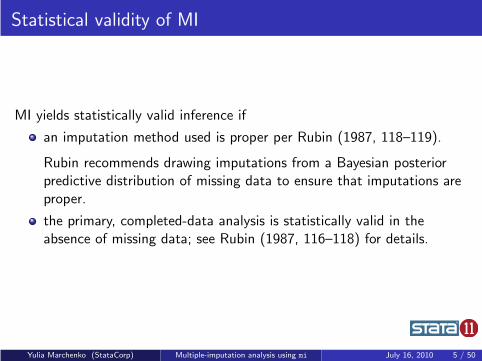
Statistical validity of MI

MI yields statistically valid inference if

an imputation method used is proper per Rubin (1987, 118–119).

Rubin recommends drawing imputations from a Bayesian posteriorpredictive distribution of missing data to ensure that imputations areproper.

the primary, completed-data analysis is statistically valid in theabsence of missing data; see Rubin (1987, 116–118) for details.


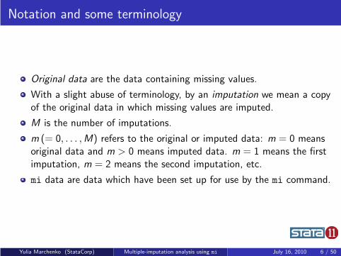
Notation and some terminology

Original data are the data containing missing values.

With a slight abuse of terminology, by an imputation we mean a copyof the original data in which missing values are imputed.

M is the number of imputations.

m (= 0, . . . ,M) refers to the original or imputed data: m = 0 meansoriginal data and m > 0 means imputed data. m = 1 means the firstimputation, m = 2 means the second imputation, etc.

mi data are data which have been set up for use by the mi command.


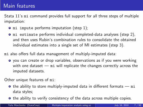
Main features

Stata 11’s mi command provides full support for all three steps of multipleimputation:

mi impute performs imputation (step 1);

mi estimate performs individual completed-data analyses (step 2),and then uses Rubin’s combination rules to consolidate the obtainedindividual estimates into a single set of MI estimates (step 3).

mi also offers full data management of multiply-imputed data:

you can create or drop variables, observations as if you were workingwith one dataset — mi will replicate the changes correctly across theimputed datasets.

Other unique features of mi:

the ability to store multiply-imputed data in different formats — mi

data styles;

the ability to verify consistency of the data across multiple copies.


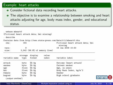
Example: heart attacks

Consider fictional data recording heart attacks.

The objective is to examine a relationship between smoking and heartattacks adjusting for age, body mass index, gender, and educationalstatus.

. webuse mheart0(Fictional heart attack data; bmi missing)

. describe

Contains data from http://www.stata-press.com/data/r11/mheart0.dtaobs: 154 Fictional heart attack data; bmi

missingvars: 9 19 Jun 2009 10:50size: 3,542 (99.9% of memory free)

storage display valuevariable name type format label variable label

attack byte %9.0g Outcome (heart attack)smokes byte %9.0g Current smokerage float %9.0g Age, in yearsbmi float %9.0g Body Mass Index, kg/m^2female byte %9.0g Genderhsgrad byte %9.0g High school graduate

(output omitted )


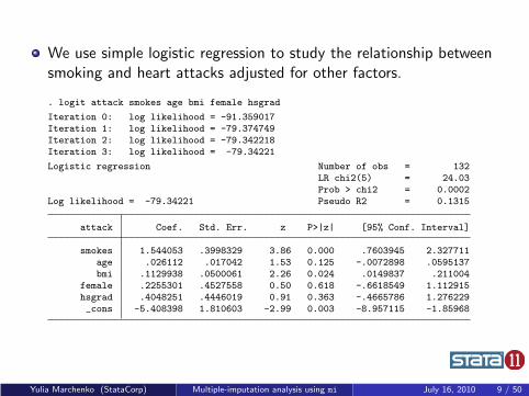
We use simple logistic regression to study the relationship betweensmoking and heart attacks adjusted for other factors.

. logit attack smokes age bmi female hsgrad

Iteration 0: log likelihood = -91.359017Iteration 1: log likelihood = -79.374749Iteration 2: log likelihood = -79.342218Iteration 3: log likelihood = -79.34221

Logistic regression Number of obs = 132LR chi2(5) = 24.03Prob > chi2 = 0.0002

Log likelihood = -79.34221 Pseudo R2 = 0.1315

attack Coef. Std. Err. z P>|z| [95% Conf. Interval]

smokes 1.544053 .3998329 3.86 0.000 .7603945 2.327711age .026112 .017042 1.53 0.125 -.0072898 .0595137bmi .1129938 .0500061 2.26 0.024 .0149837 .211004

female .2255301 .4527558 0.50 0.618 -.6618549 1.112915hsgrad .4048251 .4446019 0.91 0.363 -.4665786 1.276229_cons -5.408398 1.810603 -2.99 0.003 -8.957115 -1.85968


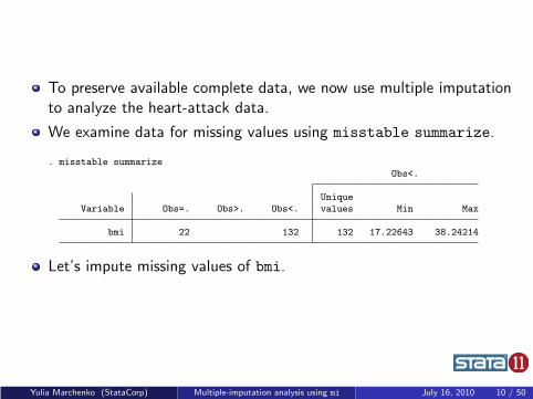
To preserve available complete data, we now use multiple imputationto analyze the heart-attack data.

We examine data for missing values using misstable summarize.

. misstable summarizeObs<.

UniqueVariable Obs=. Obs>. Obs<. values Min Max

bmi 22 132 132 17.22643 38.24214

Let’s impute missing values of bmi.


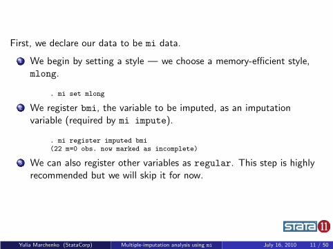
First, we declare our data to be mi data.

1 We begin by setting a style — we choose a memory-efficient style,mlong.

. mi set mlong

2 We register bmi, the variable to be imputed, as an imputationvariable (required by mi impute).

. mi register imputed bmi(22 m=0 obs. now marked as incomplete)

3 We can also register other variables as regular. This step is highlyrecommended but we will skip it for now.


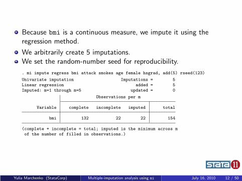
Because bmi is a continuous measure, we impute it using theregression method.

We arbitrarily create 5 imputations.

We set the random-number seed for reproducibility.

. mi impute regress bmi attack smokes age female hsgrad, add(5) rseed(123)

Univariate imputation Imputations = 5Linear regression added = 5Imputed: m=1 through m=5 updated = 0

Observations per m

Variable complete incomplete imputed total

bmi 132 22 22 154

(complete + incomplete = total; imputed is the minimum across mof the number of filled in observations.)


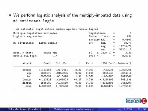
We perform logistic analysis of the multiply-imputed data usingmi estimate: logit.

. mi estimate: logit attack smokes age bmi female hsgrad

Multiple-imputation estimates Imputations = 5Logistic regression Number of obs = 154

Average RVI = 0.0564DF adjustment: Large sample DF: min = 78.77

avg = 14754.79max = 39201.13

Model F test: Equal FMI F( 5, 3527.0) = 3.39Within VCE type: OIM Prob > F = 0.0047

attack Coef. Std. Err. t P>|t| [95% Conf. Interval]

smokes 1.193653 .3579481 3.33 0.001 .492038 1.895268age .0360079 .0155205 2.32 0.020 .0055845 .0664314bmi .0985092 .0516418 1.91 0.060 -.004286 .2013044

female -.113328 .4165623 -0.27 0.786 -.9298195 .7031636hsgrad .1555202 .4034539 0.39 0.700 -.6352593 .9462997_cons -5.329907 1.800598 -2.96 0.004 -8.893172 -1.766643


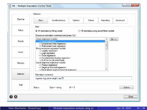
GUI — MI control panel

The MI control panel, which can be invoked from the Statistics >

Multiple imputation menu or by typing

. db mi

guides you through all the phases of MI.

(NEXT SLIDE)



Declaring data as mi

To use the mi command, your data must be declared as mi data.

To set up mi data, you need to select an mi storage style, the formatin which MI data will be stored, and register variables.

If you are going to impute data, use mi set to declare a storage style.If you already have imputed data, use mi import to import it to mi.

Use mi register to register variables.


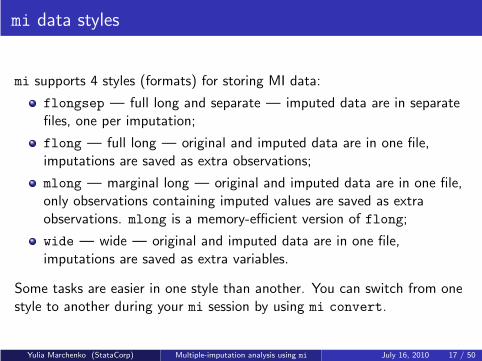
mi data styles

mi supports 4 styles (formats) for storing MI data:

flongsep — full long and separate — imputed data are in separatefiles, one per imputation;

flong — full long — original and imputed data are in one file,imputations are saved as extra observations;

mlong — marginal long — original and imputed data are in one file,only observations containing imputed values are saved as extraobservations. mlong is a memory-efficient version of flong;

wide — wide — original and imputed data are in one file,imputations are saved as extra variables.

Some tasks are easier in one style than another. You can switch from onestyle to another during your mi session by using mi convert.


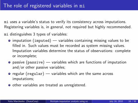
The role of registered variables in mi

mi uses a variable’s status to verify its consistency across imputations.Registering variables is, in general, not required but highly recommended.

mi distinguishes 3 types of variables:

imputation (imputed) — variables containing missing values to befilled in. Such values must be recorded as system missing values.Imputation variables determine the status of observations: completeor incomplete;

passive (passive) — variables which are functions of imputationand/or other passive variables;

regular (regular) — variables which are the same acrossimputations;

other variables are treated as unregistered.


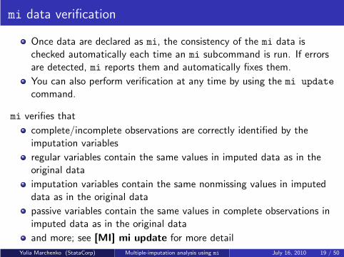
mi data verification

Once data are declared as mi, the consistency of the mi data ischecked automatically each time an mi subcommand is run. If errorsare detected, mi reports them and automatically fixes them.

You can also perform verification at any time by using the mi update

command.

mi verifies that

complete/incomplete observations are correctly identified by theimputation variables

regular variables contain the same values in imputed data as in theoriginal data

imputation variables contain the same nonmissing values in imputeddata as in the original data

passive variables contain the same values in complete observations inimputed data as in the original data

and more; see [MI] mi update for more detail


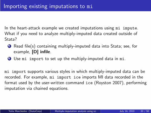
Importing existing imputations to mi

In the heart-attack example we created imputations using mi impute.What if you need to analyze multiply-imputed data created outside ofStata?

1 Read file(s) containing multiply-imputed data into Stata; see, forexample, [D] infile.

2 Use mi import to set up the multiply-imputed data in mi.

mi import supports various styles in which multiply-imputed data can berecorded. For example, mi import ice imports MI data recorded in theformat used by the user-written command ice (Royston 2007), performingimputation via chained equations.


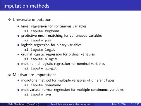
Imputation methods

Univariate imputation:

linear regression for continuous variablesmi impute regress

predictive mean matching for continuous variablesmi impute pmm

logistic regression for binary variablesmi impute logit

ordinal logistic regression for ordinal variablesmi impute ologit

multinomial logistic regression for nominal variablesmi impute mlogit

Multivariate imputation:

monotone method for multiple variables of different typesmi impute monotone

multivariate normal regression for multiple continuous variablesmi impute mvn


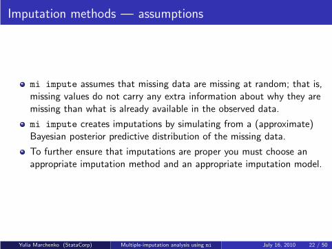
Imputation methods — assumptions

mi impute assumes that missing data are missing at random; that is,missing values do not carry any extra information about why they aremissing than what is already available in the observed data.

mi impute creates imputations by simulating from a (approximate)Bayesian posterior predictive distribution of the missing data.

To further ensure that imputations are proper you must choose anappropriate imputation method and an appropriate imputation model.


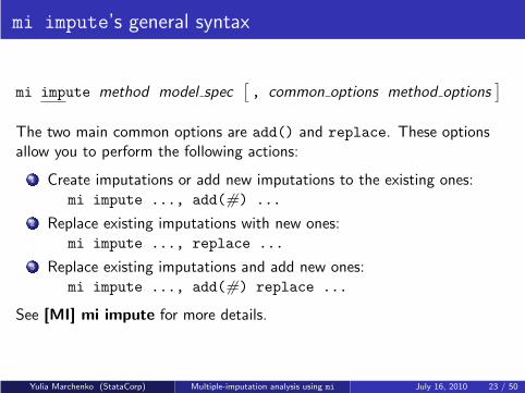
mi impute’s general syntax

mi impute method model spec[

, common options method options]

The two main common options are add() and replace. These optionsallow you to perform the following actions:

1 Create imputations or add new imputations to the existing ones:mi impute ..., add(#) ...

2 Replace existing imputations with new ones:mi impute ..., replace ...

3 Replace existing imputations and add new ones:mi impute ..., add(#) replace ...

See [MI] mi impute for more details.


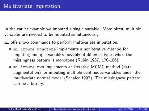
Multivariate imputation

In the earlier example we imputed a single variable. More often, multiplevariables are needed to be imputed simultaneously.

mi offers two commands to perform multivariate imputation:

mi impute monotone implements a noniterative method forimputing multiple variables possibly of different types when themissingness pattern is monotone (Rubin 1987, 170-186).

mi impute mvn implements an iterative MCMC method (dataaugmentation) for imputing multiple continuous variables under themultivariate normal model (Schafer 1997). The missingness patterncan be arbitrary.


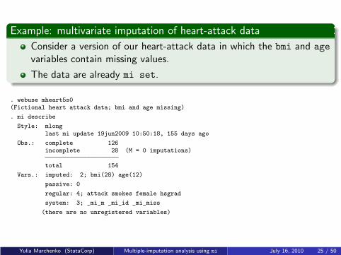
Example: multivariate imputation of heart-attack data

Consider a version of our heart-attack data in which the bmi and age

variables contain missing values.

The data are already mi set.

. webuse mheart5s0(Fictional heart attack data; bmi and age missing)

. mi describe

Style: mlonglast mi update 19jun2009 10:50:18, 155 days ago

Obs.: complete 126incomplete 28 (M = 0 imputations)

total 154

Vars.: imputed: 2; bmi(28) age(12)

passive: 0

regular: 4; attack smokes female hsgrad

system: 3; _mi_m _mi_id _mi_miss

(there are no unregistered variables)


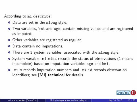
According to mi describe:

Data are set in the mlong style.

Two variables, bmi and age, contain missing values and are registeredas imputed.

Other variables are registered as regular.

Data contain no imputations.

There are 3 system variables, associated with the mlong style.

System variable mi miss records the status of observations (1 meansincomplete) based on imputation variables age and bmi.

mi m records imputation numbers and mi id records observationidentifiers; see [MI] technical for details.


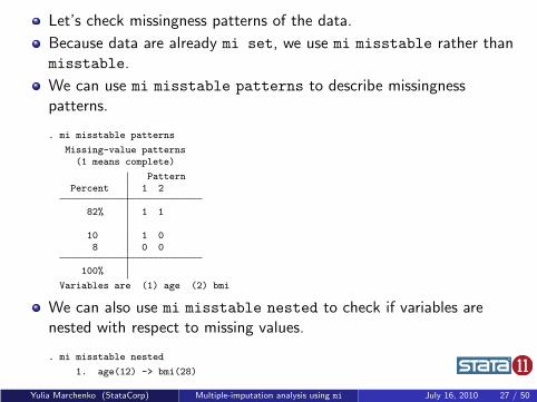
Let’s check missingness patterns of the data.

Because data are already mi set, we use mi misstable rather thanmisstable.

We can use mi misstable patterns to describe missingnesspatterns.

. mi misstable patterns

Missing-value patterns(1 means complete)

PatternPercent 1 2

82% 1 1

10 1 08 0 0

100%

Variables are (1) age (2) bmi

We can also use mi misstable nested to check if variables arenested with respect to missing values.

. mi misstable nested

1. age(12) -> bmi(28)


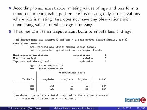
According to mi misstable, missing values of age and bmi form amonotone missing-value pattern: age is missing only in observationswhere bmi is missing. bmi does not have any observations withnonmissing values for which age is missing.

Thus, we can use mi impute monotone to impute bmi and age.

. mi impute monotone (regress) bmi age = attack smokes hsgrad female, add(5)

Conditional models:age: regress age attack smokes hsgrad femalebmi: regress bmi age attack smokes hsgrad female

Multivariate imputation Imputations = 5Monotone method added = 5Imputed: m=1 through m=5 updated = 0

age: linear regressionbmi: linear regression

Observations per m


age 142 12 12 154bmi 126 28 28 154



We used the same univariate imputation method, regress, for bothage and bmi.

We used other complete variables as explanatory variables in theimputation models.

We created 5 imputations.

Note that mi impute monotone automatically builds the appropriateconditional models.

Note that mi impute monotone automatically orders imputationvariables from the most observed to the least observed (age bmi)regardless of the order in which they are listed in the specification(bmi age).


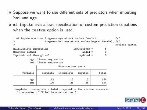
Suppose we want to use different sets of predictors when imputingbmi and age.

mi impute mvn allows specification of custom prediction equationswhen the custom option is used.

. mi impute monotone (regress age attack smokes female) ///> (regress bmi age attack smokes hsgrad female), ///> replace custom

Multivariate imputation Imputations = 5Monotone method added = 0Imputed: m=1 through m=5 updated = 5

age: linear regressionbmi: linear regression

Observations per m


age 142 12 12 154bmi 126 28 28 154



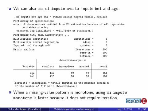
We can also use mi impute mvn to impute bmi and age.

. mi impute mvn age bmi = attack smokes hsgrad female, replace

Performing EM optimization:note: 12 observations omitted from EM estimation because of all imputation

variables missingobserved log likelihood = -651.75868 at iteration 7

Performing MCMC data augmentation ...

Multivariate imputation Imputations = 5Multivariate normal regression added = 0Imputed: m=1 through m=5 updated = 5

Prior: uniform Iterations = 500burn-in = 100between = 100

Observations per m


age 142 12 12 154bmi 126 28 28 154


When a missing-value pattern is monotone, using mi impute

monotone is faster because it does not require iteration.


mi impute mvn uses data augmentation, an iterative MCMC method,to impute missing values under a multivariate normal model.

mi impute mvn uses estimates from the EM algorithm as startingvalues for the MCMC procedure. You can supply your own initialvalues, if needed, using option initmcmc().

The default prior is uniform under which posterior mode estimatesand maximum-likelihood estimates are equivalent. You can changethe default prior specification using option prior().

The first imputation is drawn after an initial default burn-in period of100 iterations. You can use option burnin() to choose a differentburn-in period.

The subsequent imputations are drawn every 100 (the default)iterations apart. You can change the number of iterations betweenimputations using option burnbetween().


Estimation using multiple imputation

mi estimate performs analysis of multiply-imputed data.

mi estimate requires mi data with at least 2 imputations.

Basic syntax:

mi estimate[

, options]

: estimation command

mi estimate runs estimation command on all imputed data andreports the MI estimates of coefficients and their standard errors.

estimation command is one of the supported estimation commands aslisted in [MI] estimation.


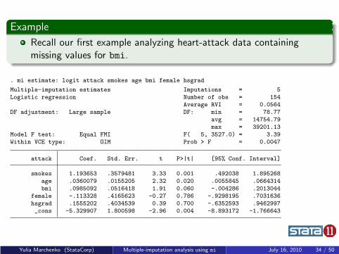
Example

Recall our first example analyzing heart-attack data containingmissing values for bmi.

. mi estimate: logit attack smokes age bmi female hsgrad



avg = 14754.79max = 39201.13

Model F test: Equal FMI F( 5, 3527.0) = 3.39Within VCE type: OIM Prob > F = 0.0047


smokes 1.193653 .3579481 3.33 0.001 .492038 1.895268age .0360079 .0155205 2.32 0.020 .0055845 .0664314bmi .0985092 .0516418 1.91 0.060 -.004286 .2013044

female -.113328 .4165623 -0.27 0.786 -.9298195 .7031636hsgrad .1555202 .4034539 0.39 0.700 -.6352593 .9462997_cons -5.329907 1.800598 -2.96 0.004 -8.893172 -1.766643


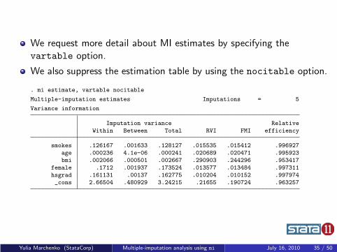
We request more detail about MI estimates by specifying thevartable option.

We also suppress the estimation table by using the nocitable option.

. mi estimate, vartable nocitable

Multiple-imputation estimates Imputations = 5

Variance information

Imputation variance RelativeWithin Between Total RVI FMI efficiency

smokes .126167 .001633 .128127 .015535 .015412 .996927age .000236 4.1e-06 .000241 .020689 .020471 .995923bmi .002066 .000501 .002667 .290903 .244296 .953417

female .1712 .001937 .173524 .013577 .013484 .997311hsgrad .161131 .00137 .162775 .010204 .010152 .997974_cons 2.66504 .480929 3.24215 .21655 .190724 .963257


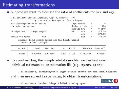
Estimating transformations

Suppose we want to estimate the ratio of coefficients for bmi and age.

. mi estimate (ratio: _b[bmi]/_b[age]), nocoef: ///> logit attack smokes age bmi female hsgrad



avg = 376.39Within VCE type: OIM max = 376.39

command: logit attack smokes age bmi female hsgradratio: _b[bmi]/_b[age]


ratio 2.720908 1.679848 1.62 0.106 -.5821547 6.02397

To avoid refitting the completed-data models, we can first saveindividual estimates to an estimation file (e.g., myest.ster):

. mi estimate, saving(myest): logit attack smokes age bmi female hsgrad

and then use mi estimate using to obtain transformations:

. mi estimate (ratio: b[age]/ b[bmi]) using myest


Testing hypotheses

After mi estimate, you can use

mi test to test the subset of coefficients equal to zero;

mi testtransform to test other linear or nonlinear hypotheses.

mi test and mi testtransform provide

the conditional (equal fraction-missing-information, FMI) test of Li etal. (1991);

the unconditional test of Rubin (1987, 77–78). This test may bepreferable when the number of imputations is large and the equal FMIassumption is suspect.

small-sample adjustments for the tests as described in Marchenko andReiter (2009).


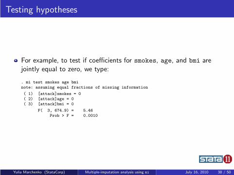
Testing hypotheses

For example, to test if coefficients for smokes, age, and bmi arejointly equal to zero, we type:

. mi test smokes age bminote: assuming equal fractions of missing information

( 1) [attack]smokes = 0( 2) [attack]age = 0( 3) [attack]bmi = 0

F( 3, 674.9) = 5.46Prob > F = 0.0010


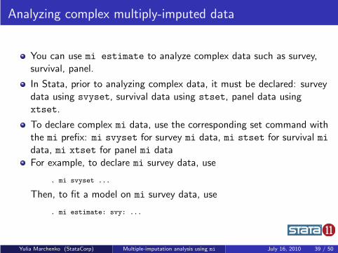
Analyzing complex multiply-imputed data

You can use mi estimate to analyze complex data such as survey,survival, panel.

In Stata, prior to analyzing complex data, it must be declared: surveydata using svyset, survival data using stset, panel data usingxtset.

To declare complex mi data, use the corresponding set command withthe mi prefix: mi svyset for survey mi data, mi stset for survival midata, mi xtset for panel mi data

For example, to declare mi survey data, use

. mi svyset ...

Then, to fit a model on mi survey data, use

. mi estimate: svy: ...


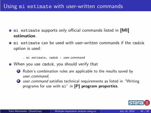
Using mi estimate with user-written commands

mi estimate supports only official commands listed in [MI]estimation.

mi estimate can be used with user-written commands if the cmdok

option is used:

. mi estimate, cmdok : user command

When you use cmdok, you should verify that

1 Rubin’s combination rules are applicable to the results saved byuser command;

2 user command satisfies technical requirements as listed in “Writingprograms for use with mi” in [P] program properties.


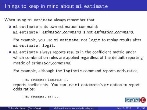
Things to keep in mind about mi estimate

When using mi estimate always remember that

mi estimate is its own estimation command:mi estimate: estimation command is not estimation command.

For example, you use mi estimate, not logit to replay results aftermi estimate: logit.

mi estimate always reports results in the coefficient metric underwhich combination rules are applied regardless of the default reportingmetric of estimation command.

For example, although the logistic command reports odds ratios,

. mi estimate: logistic ...

reports coefficients. You can use mi estimate’s or option to reportodds ratios:

. mi estimate, or: ...


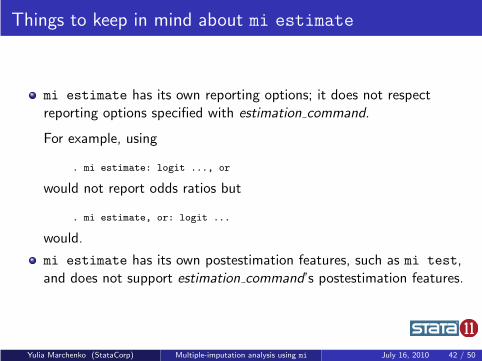
Things to keep in mind about mi estimate

mi estimate has its own reporting options; it does not respectreporting options specified with estimation command.

For example, using

. mi estimate: logit ..., or

would not report odds ratios but

. mi estimate, or: logit ...

would.

mi estimate has its own postestimation features, such as mi test,and does not support estimation command’s postestimation features.


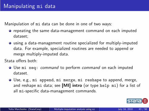
Manipulating mi data

Manipulation of mi data can be done in one of two ways:

repeating the same data-management command on each imputeddataset;

using a data-management routine specialized for multiply-imputeddata. For example, specialized routines are needed to append ormerge multiply-imputed data.

Stata offers both:

Use mi xeq: command to perform command on each imputeddataset.

Use, e.g., mi append, mi merge, mi reshape to append, merge,and reshape mi data; see [MI] intro (or type help mi) for a list ofall mi-specific data-management commands.


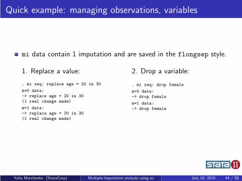
Quick example: managing observations, variables

mi data contain 1 imputation and are saved in the flongsep style.

1. Replace a value:

. mi xeq: replace age = 20 in 30

m=0 data:-> replace age = 20 in 30(1 real change made)

m=1 data:-> replace age = 20 in 30(1 real change made)

2. Drop a variable:

. mi xeq: drop female

m=0 data:-> drop female

m=1 data:-> drop female


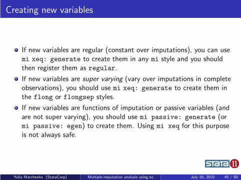
Creating new variables

If new variables are regular (constant over imputations), you can usemi xeq: generate to create them in any mi style and you shouldthen register them as regular.

If new variables are super varying (vary over imputations in completeobservations), you should use mi xeq: generate to create them inthe flong or flongsep styles.

If new variables are functions of imputation or passive variables (andare not super varying), you should use mi passive: generate (ormi passive: egen) to create them. Using mi xeq for this purposeis not always safe.


Managing imputations

You can use

mi impute to create or add new imputations;

mi set m to delete selected imputations;

mi add to add imputations from a separate file;

mi set M to reset the number of imputations (or create emptyimputations in which missing data are not filled in).


Other useful commands

Use mi query to get a short summary of the mi settings.

Use mi describe to get a more detailed report about mi data.

Use mi varying to identify variables that vary over imputations.

For example, you can use it to identify imputation and passivevariables and then register them using mi register. This commandalso helps to detect potential problems.


Things to remember about data manipulation

When performing data manipulation on mi data, remember

to use the mi versions of the data-management routines, if they exist;

to use mi xeq with routines for which there is no mi prefix;

to run mi update periodically to ensure consistency of the mi data.


Summary

mi accommodates all steps of the MI technique:

mi impute provides univariate and multivariate methods for filling inmissing values;mi estimate performs completed-data analysis and combinesestimates using Rubin’s pooling rules.

mi provides full data-management support.

mi provides 4 styles for storing MI data and can import from 5 styles.

mi verifies consistency of your data at every opportunity.

mi offers postestimation features: testing linear or nonlinearhypotheses.

mi provides elaborate GUI support — MI control panel.

mi offers extensive documentation, manual [MI] Multipleimputation.


References

Li, K.-H., T. E. Raghunathan, and D. B. Rubin. 1991. Large-samplesignificance levels from multiply imputed data using moment-basedstatistics and an F reference distribution. Journal of the American

Statistical Association 86: 1065—1073.

Marchenko, Y. V. and J. P. Reiter. 2009. Improved degrees of freedom formultivariate significance tests obtained from multiply imputed,small-sample data. Stata Journal 9: 388—397.

Royston, P. 2007. Multiple imputation of missing values: Further updateof ice, with an emphasis on interval censoring. Stata Journal 7: 445—464.

Rubin, D. B. 1987. Multiple Imputation for Nonresponse in Surveys. NewYork: Wiley.

Rubin, D. B. 1996. Multiple imputation after 18+ years. Journal of the

American Statistical Association 91: 473—489.

Schafer, J. L. 1997. Analysis of Incomplete Multivariate Data. BocaRaton, FL: Chapman & Hall/CRC.


Documents

Multiple-imputation analysis using Stata's mi command · mi estimateperforms individual completed-data analyses (step 2), and then uses Rubin’s combination rules to consolidate