Multiple Factor Analysis (MFA) - University of Texas at Dallasherve/Abdi-MFA2007-pretty.pdf · Multiple factor analysis (MFA, see Escoﬁer and Pagès, 1990, 1994) analyzes observations

LATEX document: Abdi-MFA2007-pretty.tex - page 1April 28, 2009 - 14h56

\paperwidth: 455.24408pt (160mm)\paperheight: 682.86613pt (240mm)

\textwidth: 327.20668pt (115mm)\textheight: 540.60236pt (190mm)

\topmargin: 19.91692pt (7mm)\oddsidemargin: 34.1433pt (12mm)

Multiple Factor Analysis(MFA)

Hervé Abdi1 & Dominique Valentin

1 Overview

1.1 Origin and goal of the method

Multiple factor analysis (MFA, see Escofier and Pagès, 1990, 1994)analyzes observations described by several “blocks" or sets of vari-ables. MFA seeks the common structures present in all or some ofthese sets. MFA is performed in two steps. First a principal com-ponent analysis (PCA) is performed on each data set which is then“normalized” by dividing all its elements by the square root of thefirst eigenvalue obtained from of its PCA. Second, the normalizeddata sets are merged to form a unique matrix and a global PCA isperformed on this matrix. The individual data sets are then pro-jected onto the global analysis to analyze communalities and dis-crepancies. MFA is used in very different domains such as sensoryevaluation, economy, ecology, and chemistry.

1In: Neil Salkind (Ed.) (2007). Encyclopedia of Measurement and Statistics.Thousand Oaks (CA): Sage.Address correspondence to: Hervé AbdiProgram in Cognition and Neurosciences, MS: Gr.4.1,The University of Texas at Dallas,Richardson, TX 75083–0688, USAE-mail: [email protected] http://www.utd.edu/∼herve

1





H. Abdi & D. Valentin: Multiple Factor Analysis

1.2 When to use it

MFA is used to analyze a set of observations described by severalgroups of variables. The number of variables in each group maydiffer and the nature of the variables (nominal or quantitative) canvary from one group to the other but the variables should be of thesame nature in a given group. The analysis derives an integratedpicture of the observations and of the relationships between thegroups of variables.

1.3 The main idea

The goal of MFA is to integrate different groups of variables de-scribing the same observations. In order to do so, the first step is tomake these groups of variables comparable. Such a step is neededbecause the straightforward analysis obtained by concatenatingall variables would be dominated by the group with the strongeststructure. A similar problem can occur in a non-normalized PCA:without normalization, the structure is dominated by the variableswith the largest variance. For PCA, the solution is to normalize(i.e., to use Z -scores) each variable by dividing it by its standarddeviation. The solution proposed by MFA is similar: To comparegroups of variables, each group is normalized by dividing all itselements by a quantity called its first singular value which is thematrix equivalent of the standard deviation. Practically, This stepis implemented by performing a PCA on each group of variables.The first singular value is the square root of the first eigenvalue ofthe PCA. After normalization, the data tables are concatenated intoa data table which is submitted to PCA.

2 An example

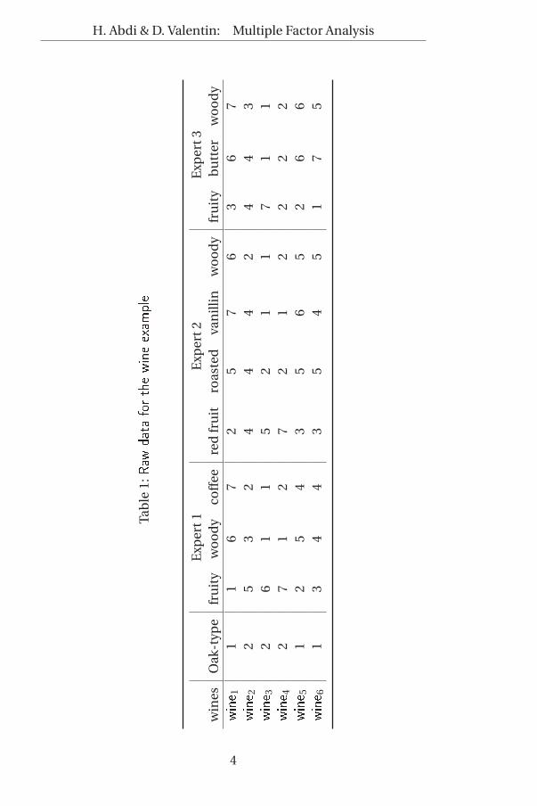
To illustrate MFA, we selected six wines, coming from the same har-vest of Pinot Noir, aged in six different barrels made with one oftwo different types of oak. Wines 1, 5, and 6 were aged with the firsttype of oak, and wines 2, 3, and 4 with the second. Next, we askedeach of three wine experts to choose from two to five variables to

2






describe the six wines. For each wine, the expert rated the inten-sity of the variables on a 9-point scale. The results are presentedin Table 1 (the same example is used in the entry for STATIS). Thegoal of the analysis is twofold. First we want to obtain a typologyof the wines and second we want to know if there is an agreementbetween the experts.

3 Notations

The raw data consist in T data sets. Each data set is called a study.Each study is an I× J[t ] rectangular data matrix denoted Y[t ], whereI is the number of observations and J[t ] the number of variables ofthe t-th study. Each data matrix is, in general, preprocessed (e.g.,centered, normalized) and the preprocessed data matrices actu-ally used in the analysis are denoted X[t ].

For our example, the data consist in T = 3 studies. The data(from Table 1) were centered by column (i.e., the mean of each col-umn is zero) and normalized (i.e., for each column, the sum of thesquared elements is equal to 1). So, the starting point of the analy-sis consists in three matrices:

X[1] =

−0.57 0.58 0.760.19 −0.07 −0.280.38 −0.50 −0.480.57 −0.50 −0.28

−0.38 0.36 0.14−0.19 0.14 0.14

,

X[2] =

−0.50 0.35 0.57 0.540.00 0.05 0.03 −0.320.25 −0.56 −0.51 −0.540.75 −0.56 −0.51 −0.32

−0.25 0.35 0.39 0.32−0.25 0.35 0.03 0.32

,

and

3






Tab

le1:

Raw

data

fort

hewine

exam

ple

Exp

ert1

Exp

ert2

Exp

ert3

win

esO

ak-t

ype

fru

ity

wo

od

yco

ffee

red

fru

itro

aste

dva

nill

inw

oo

dy

fru

ity

bu

tter

wo

od

ywine

11

16

72

57

63

67

wine

22

53

24

44

24

43

wine

32

61

15

21

17

11

wine

42

71

27

21

22

22

wine

51

25

43

56

52

66

wine

61

34

43

54

51

75

4






X[3] =

−0.03 0.31 0.570.17 −0.06 −0.190.80 −0.61 −0.57

−0.24 −0.43 −0.38−0.24 0.31 0.38−0.45 0.49 0.19

. (1)

Each observation is assigned a mass which reflects its impor-tance. When all observations have the same importance, their ma-sses are all equal to mi = 1

I . The set of the masses is stored in anI × I diagonal matrix denoted M.

4 Finding the global space

4.1 Computing the separate PCA’s

To normalize the studies, we first compute a PCA for each study.The first singular value (i.e., the square root of the first eigenvalue)is the normalizing factor used to divide the elements of the data ta-ble. For example, the PCA of the first group gives a first eigenvalue

1%1 = 2.86 and a first singular value of 1ϕ1 =p1%1 = 1.69. This gives

the first normalized data matrix denoted Z[1]:

Z[1] = 1ϕ−11 ×X[1] =

−0.33 0.34 0.450.11 −0.04 −0.160.22 −0.30 −0.280.33 −0.30 −0.16

−0.22 0.21 0.08−0.11 0.08 0.08

. (2)

Matrices Z[2] and Z[3] are normalized with their first respectivesingular values of 2ϕ1 = 1.91 and 3ϕ1 = 1.58. Normalized matriceshave a first singular value equal to 1.

5






4.2 Building the global matrix

The normalized studies are concatenated into an I×T matrix calledthe global data matrix denoted Z. Here we obtain:

Z = [Z[1] Z[2] Z[3]

]

=

−0.33 0.34 0.45 −0.26 0.18 0.30 0.28 −0.02 0.19 0.360.11 −0.04 −0.16 0.00 0.03 0.02 −0.17 0.11 −0.04 −0.120.22 −0.30 −0.28 0.13 −0.29 −0.27 −0.28 0.51 −0.39 −0.360.33 −0.30 −0.16 0.39 −0.29 −0.27 −0.17 −0.15 −0.27 −0.24

−0.22 0.21 0.08 −0.13 0.18 0.20 0.17 −0.15 0.19 0.24−0.11 0.08 0.08 −0.13 0.18 0.02 0.17 −0.29 0.31 0.12

.

(3)

4.3 Computing the global PCA

To analyze the global matrix, we use standard PCA. This amountsto computing the singular value decomposition of the global datamatrix:

Z = U∆VT with UTU = VTV = I , (4)

(where U and V are the left and right singular vectors of Z and ∆ isthe diagonal matrix of the singular values).

For our example we obtain:

U =

0.53 −0.35 −0.58 −0.04 0.31−0.13 −0.13 0.49 0.51 0.54−0.56 −0.57 0.01 −0.36 −0.25−0.44 0.62 −0.48 0.15 0.03

0.34 0.04 0.16 0.39 −0.730.27 0.40 0.40 −0.65 0.11

(5)

and

diag {∆} = [1.68 0.60 0.34 0.18 0.11

]

and diag {Λ} = diag{∆2}= [

2.83 0.36 0.11 0.03 0.01]

(6)

6






(Λ gives the eigenvalues of the PCA) and

V =

−0.34 0.22 0.03 0.14 0.550.35 −0.14 −0.03 0.30 0.020.32 −0.06 −0.65 −0.24 0.60

−0.28 0.34 −0.32 0.31 −0.180.30 −0.00 0.43 0.11 0.190.30 −0.18 −0.00 0.67 0.110.30 0.09 −0.22 −0.36 −0.38

−0.22 −0.86 0.01 −0.12 −0.000.36 0.20 0.45 −0.30 0.190.37 0.01 −0.21 0.18 −0.28

(7)

The global factor scores for the wines are obtained as:

F = M− 12 U∆ (8)

=

2.18 −0.51 −0.48 −0.02 0.08−0.56 −0.20 0.41 0.23 0.15−2.32 −0.83 0.01 −0.16 −0.07−1.83 0.90 −0.40 0.07 0.01

1.40 0.05 0.13 0.17 −0.201.13 0.58 0.34 −0.29 0.03

. (9)

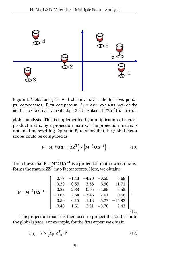
In F, each row represents an observation (i.e., a wine) and eachcolumn a component. Figure 1 displays the wines in the spaceof the first two principal components. The first component hasan eigenvalue equal to λ1 = 2.83, which corresponds to 84% ofthe inertia

( 2.832.83+0.36+0.11+0.03+0.01 = 2.83

3.35 ≈ .84). The second compo-

nent, with an eigenvalue of .36, explains 11% of the inertia. Thefirst component is interpreted as the opposition between the first(wines 1, 5, and 6) and the second oak type (wines 2, 3, and 4).

5 Partial analyses

The global analysis reveals the common structure of the wine space.In addition, we want to see how each expert “interprets" this space.This is achieved by projecting the data set of each expert onto the

7






4

3

21

5

6

Figure 1: Global analysis: Plot of the wines on the �rst two princi-pal components. First component: λ1 = 2.83, explains 84% of theinertia, Second component: λ2 = 2.83, explains 11% of the inertia.

global analysis. This is implemented by multiplication of a crossproduct matrix by a projection matrix. The projection matrix isobtained by rewriting Equation 8, to show that the global factorscores could be computed as

F = M− 12 U∆=

(ZZT

)×

(M− 1

2 U∆−1)

. (10)

This shows that P = M− 12 U∆−1 is a projection matrix which trans-

forms the matrix ZZT into factor scores. Here, we obtain:

P = M− 12 U∆−1 =

0.77 −1.43 −4.20 −0.55 6.68−0.20 −0.55 3.56 6.90 11.71−0.82 −2.33 0.05 −4.85 −5.53−0.65 2.54 −3.46 2.01 0.66

0.50 0.15 1.13 5.27 −15.930.40 1.61 2.91 −8.78 2.43

,

(11)The projection matrix is then used to project the studies onto

the global space. For example, for the first expert we obtain

F[1] = T ×(Z[1]Z

T[1]

)P (12)

8






=

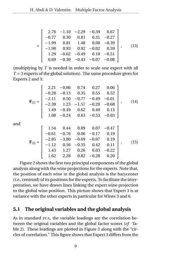
2.76 −1.10 −2.29 −0.39 0.67−0.77 0.30 0.81 0.31 −0.27−1.99 0.81 1.48 0.08 −0.39−1.98 0.93 0.92 −0.02 0.59

1.29 −0.62 −0.49 0.10 −0.510.69 −0.30 −0.43 −0.07 −0.08

, (13)

(multiplying by T is needed in order to scale one expert with allT = 3 experts of the global solution). The same procedure gives forExperts 2 and 3:

F[2] =

2.21 −0.86 0.74 0.27 0.06−0.28 −0.13 0.35 0.55 0.52−2.11 0.50 −0.77 −0.49 −0.01−2.39 1.23 −1.57 −0.20 −0.68

1.49 −0.49 0.62 0.40 0.131.08 −0.24 0.63 −0.53 −0.03

, (14)

and

F[3] =

1.54 0.44 0.09 0.07 −0.47−0.61 −0.76 0.06 −0.17 0.19−2.85 −3.80 −0.69 −0.07 0.19−1.12 0.56 −0.55 0.42 0.11

1.43 1.27 0.26 0.03 −0.221.62 2.28 0.82 −0.28 0.20

. (15)

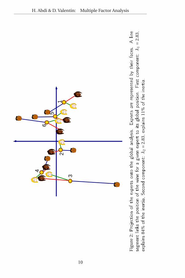
Figure 2 shows the first two principal components of the globalanalysis along with the wine projections for the experts. Note that,the position of each wine in the global analysis is the barycenter(i.e., centroid) of its positions for the experts. To facilitate the inter-pretation, we have drawn lines linking the expert wine projectionto the global wine position. This picture shows that Expert 3 is atvariance with the other experts in particular for Wines 3 and 6.

5.1 The original variables and the global analysis

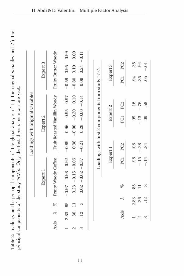
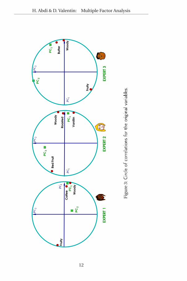
As in standard PCA, the variable loadings are the correlation be-tween the original variables and the global factor scores (cf. Ta-ble 2). These loadings are plotted in Figure 3 along with the “cir-cles of correlation.” This figure shows that Expert 3 differs from the

9






21

46

5

3

Fig

ure

2:Projectio

nof

theexperts

onto

theglo

bala

nalys

is.Ex

perts

arerepresentedby

their

faces.

Aline

segm

entlink

sthepo

sition

ofthewine

fora

given

expert

toits

globalp

osition

.First

compo

nent:λ

1=

2.83,

expla

ins84

%of

theine

rtia,

Second

compo

nent:λ

2=

2.83,e

xplains

11%

oftheine

rtia.

10





H. Abdi & D. Valentin: Multiple Factor AnalysisTa

ble

2:Lo

ading

son

theprinc

ipalc

ompo

nentsof

theglo

bala

nalys

isof

1.)theoriginalv

ariab

lesand2.)the

princ

ipalc

ompo

nentso

fthe

study

pca's.

Only

the�rst

threedim

ensio

nsarekept.

Load

ings

wit

ho

rigi

nal

vari

able

s

Exp

ert1

Exp

ert2

Exp

ert3

Axi

sλ

%Fr

uit

yW

oo

dy

Co

ffee

Fru

itR

oas

ted

Van

illin

Wo

od

yFr

uit

yB

utt

erW

oo

dy

12.

8385

−0.9

70.

980.

92−0

.89

0.96

0.95

0.97

−0.5

90.

950.

99

2.3

611

0.23

−0.1

5−0

.06

0.38

−0.0

0−0

.20

0.10

−0.8

00.

190.

00

3.1

23

0.02

−0.0

2−0

.37

−0.2

10.

28−0

.00

−0.1

40.

080.

24−0

.11

Load

ings

wit

hfi

rst2

com

po

nen

tsfr

om

stu

dy

PC

A’s

Exp

ert1

Exp

ert2

Exp

ert3

Axi

sλ

%P

C1

PC

2P

C1

PC

2P

C1

PC

2

12.

8385

.98

.08

.99

−.16

.94

−.35

2.3

611

−.15

−.28

−.13

−.76

.35

.94

3.1

23

−.14

.84

.09

.58

.05

−.01

11






EX

PER

T 1

Wo

od

y1

PC

1

PC

2

PC

2

Fru

ity

Co

ffe

e

PC

EX

PER

T 2

11

PC

2

PC

PC

PC

2

Va

nillin

Ro

ast

ed

Wo

od

yR

ed

Fru

it

EX

PER

T 3

Bu

tte

r

1

PC

1

PC

2

PC

2

Fru

ity

Wo

od

yP

C

Fig

ure

3:Circle

ofcorre

lation

sfor

theoriginalv

ariab

les.

12






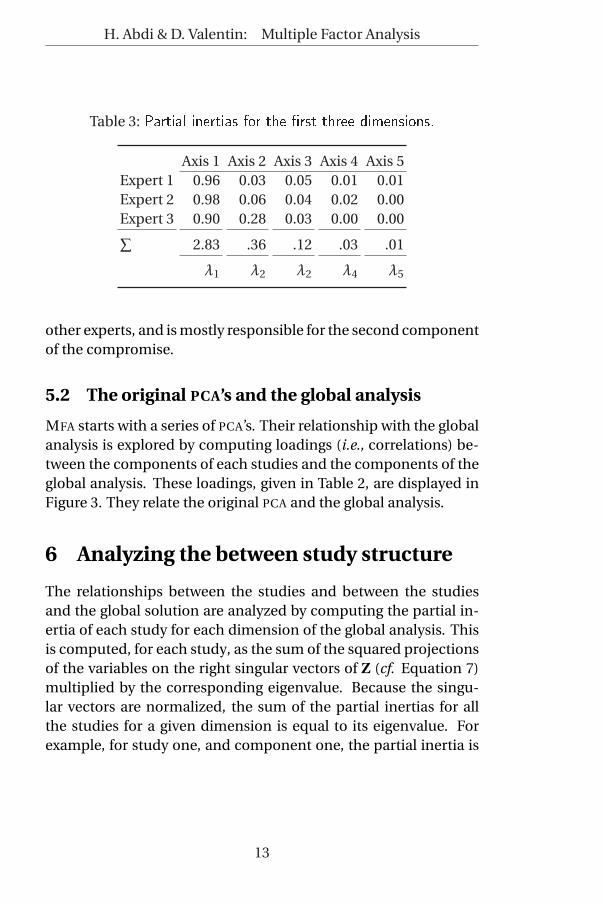
Table 3: Partial inertias for the �rst three dimensions.

Axis 1 Axis 2 Axis 3 Axis 4 Axis 5Expert 1 0.96 0.03 0.05 0.01 0.01Expert 2 0.98 0.06 0.04 0.02 0.00Expert 3 0.90 0.28 0.03 0.00 0.00∑

2.83 .36 .12 .03 .01

λ1 λ2 λ2 λ4 λ5

other experts, and is mostly responsible for the second componentof the compromise.

5.2 The original PCA’s and the global analysis

MFA starts with a series of PCA’s. Their relationship with the globalanalysis is explored by computing loadings (i.e., correlations) be-tween the components of each studies and the components of theglobal analysis. These loadings, given in Table 2, are displayed inFigure 3. They relate the original PCA and the global analysis.

6 Analyzing the between study structure

The relationships between the studies and between the studiesand the global solution are analyzed by computing the partial in-ertia of each study for each dimension of the global analysis. Thisis computed, for each study, as the sum of the squared projectionsof the variables on the right singular vectors of Z (cf. Equation 7)multiplied by the corresponding eigenvalue. Because the singu-lar vectors are normalized, the sum of the partial inertias for allthe studies for a given dimension is equal to its eigenvalue. Forexample, for study one, and component one, the partial inertia is

13






Dimension 11

λ = 2.831

22λ = 0.36

τ = 11%

τ = 85%

Dim

en

sio

n 2

1

3

2

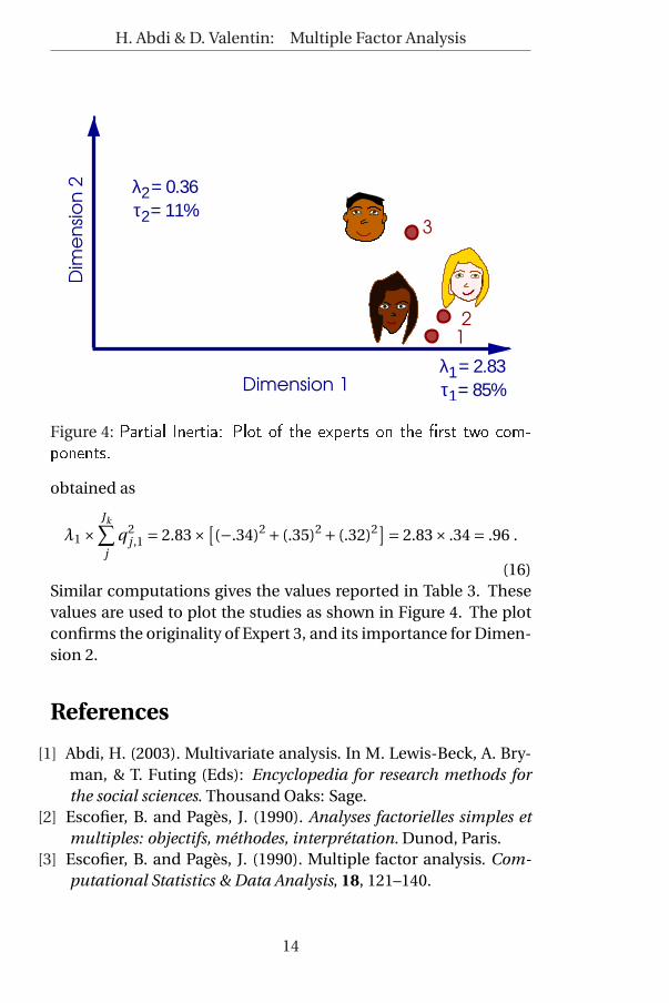
Figure 4: Partial Inertia: Plot of the experts on the �rst two com-ponents.

obtained as

λ1 ×Jk∑j

q2j ,1 = 2.83× [

(−.34)2 + (.35)2 + (.32)2]= 2.83× .34 = .96 .

(16)Similar computations gives the values reported in Table 3. Thesevalues are used to plot the studies as shown in Figure 4. The plotconfirms the originality of Expert 3, and its importance for Dimen-sion 2.

References

[1] Abdi, H. (2003). Multivariate analysis. In M. Lewis-Beck, A. Bry-man, & T. Futing (Eds): Encyclopedia for research methods forthe social sciences. Thousand Oaks: Sage.

[2] Escofier, B. and Pagès, J. (1990). Analyses factorielles simples etmultiples: objectifs, méthodes, interprétation. Dunod, Paris.

[3] Escofier, B. and Pagès, J. (1990). Multiple factor analysis. Com-putational Statistics & Data Analysis, 18, 121–140.

14

Documents

Multiple Factor Analysis (MFA) - University of Texas at Dallasherve/Abdi-MFA2007-pretty.pdf · Multiple factor analysis (MFA, see Escoﬁer and Pagès, 1990, 1994) analyzes observations