Multiple Factor Analysis - Freefactominer.free.fr/course/doc/MFA_course_slides.pdfMultiple Factor Analysis ... IntroductionEquilibrium and global PCAStudying groupsFurther topics

Data - Introduction Equilibrium and global PCA Studying groups Further topics

Multiple Factor Analysis

François Husson

Applied Mathematics Department - Rennes Agrocampus

[email protected]

1 / 39


Outline

1 Data - Introduction

2 Equilibrium and global PCA

3 Studying groupsGroup representationPartial points representationSeparate analyses

4 Further topicsQualitative dataContingency tablesInterpretation aids

2 / 39


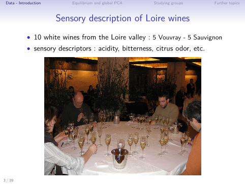
Sensory description of Loire wines

• 10 white wines from the Loire valley : 5 Vouvray - 5 Sauvignon• sensory descriptors : acidity, bitterness, citrus odor, etc.

3 / 39


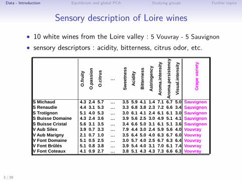
Sensory description of Loire wines

• 10 white wines from the Loire valley : 5 Vouvray - 5 Sauvignon• sensory descriptors : acidity, bitterness, citrus odor, etc.

O.f

ruit

y

O.p

as

sio

n

O.c

itru

s

…

Sw

eetn

ess

Ac

idit

y

Bit

tern

es

s

As

trin

ge

nc

y

Aro

ma

.in

ten

sit

y

Aro

ma

.pe

rsis

ten

cy

Vis

ua

l.in

ten

sit

y

Gra

pe v

arie

ty

S Michaud 4.3 2.4 5.7 … 3.5 5.9 4.1 1.4 7.1 6.7 5.0 Sauvignon

S Renaudie 4.4 3.1 5.3 … 3.3 6.8 3.8 2.3 7.2 6.6 3.4 Sauvignon

S Trotignon 5.1 4.0 5.3 … 3.0 6.1 4.1 2.4 6.1 6.1 3.0 Sauvignon

S Buisse Domaine 4.3 2.4 3.6 … 3.9 5.6 2.5 3.0 4.9 5.1 4.1 Sauvignon

S Buisse Cristal 5.6 3.1 3.5 … 3.4 6.6 5.0 3.1 6.1 5.1 3.6 Sauvignon

V Aub Silex 3.9 0.7 3.3 … 7.9 4.4 3.0 2.4 5.9 5.6 4.0 Vouvray

V Aub Marigny 2.1 0.7 1.0 … 3.5 6.4 5.0 4.0 6.3 6.7 6.0 Vouvray

V Font Domaine 5.1 0.5 2.5 … 3.0 5.7 4.0 2.5 6.7 6.3 6.4 Vouvray

V Font Brûlés 5.1 0.8 3.8 … 3.9 5.4 4.0 3.1 7.0 6.1 7.4 Vouvray

V Font Coteaux 4.1 0.9 2.7 … 3.8 5.1 4.3 4.3 7.3 6.6 6.3 Vouvray

3 / 39


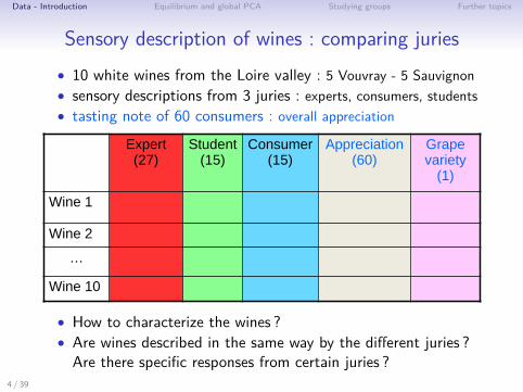
Sensory description of wines : comparing juries• 10 white wines from the Loire valley : 5 Vouvray - 5 Sauvignon• sensory descriptions from 3 juries : experts, consumers, students• tasting note of 60 consumers : overall appreciation

Expert(27)

Student(15)

Consumer(15)

Appreciation(60)

Grapevariety

(1)

Wine 1

Wine 2

…

Wine 10

• How to characterize the wines ?• Are wines described in the same way by the different juries ?Are there specific responses from certain juries ?

4 / 39


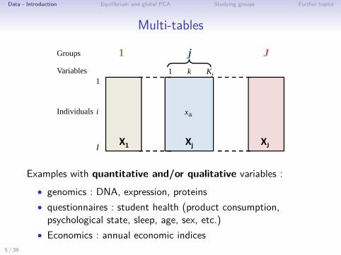
Multi-tables

1

i

I

1

1 k Kj

xik

j J

X1 Xj XJ

Individuals

Variables

Groups

Examples with quantitative and/or qualitative variables :• genomics : DNA, expression, proteins• questionnaires : student health (product consumption,psychological state, sleep, age, sex, etc.)

• Economics : annual economic indices5 / 39


Aims

• Study the similarity between individuals with respect to thewhole set of variables AND the relationships between variables

Take the group structure into account• Study the overall similarities and differences between groups(and the specific features of each group)

• Study the similarities and differences between groups from anindividual’s point of view

• Compare the characteristics of individuals from the separateanalyses

⇒ Balance the influence of all of the groupsin the analysis

6 / 39


Outline





7 / 39


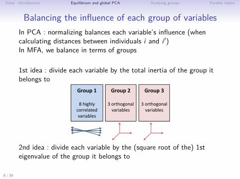
Balancing the influence of each group of variablesIn PCA : normalizing balances each variable’s influence (whencalculating distances between individuals i and i ′)In MFA, we balance in terms of groups

1st idea : divide each variable by the total inertia of the group itbelongs to

Group 1

8 highly

correlated

variables

Group 2

3 orthogonal

variables

Group 3

3 orthogonal

variables

2nd idea : divide each variable by the (square root of the) 1steigenvalue of the group it belongs to

8 / 39


Balancing the influence of each group of variables

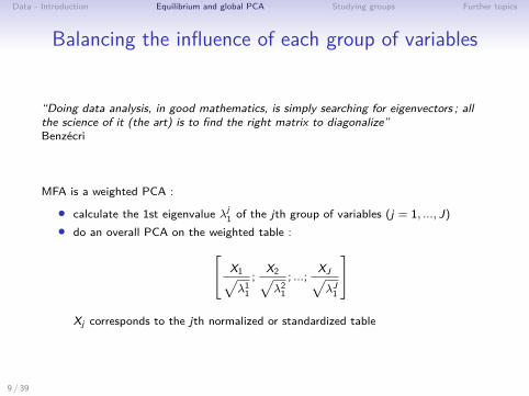
“Doing data analysis, in good mathematics, is simply searching for eigenvectors ; allthe science of it (the art) is to find the right matrix to diagonalize”Benzécri

MFA is a weighted PCA :

• calculate the 1st eigenvalue λj1 of the jth group of variables (j = 1, ..., J)• do an overall PCA on the weighted table :[

X1√λ1

1

;X2√λ2

1

; ...;XJ√λJ1

]

Xj corresponds to the jth normalized or standardized table

9 / 39


Balancing the influence of each group of variables

Before weighting After weightingExpert Student Consumer Expert Student Consumer

λ1 11.74 7.89 7.17 1.00 1.00 1.00λ2 6.78 3.83 2.59 0.58 0.49 0.36λ3 2.74 1.70 1.63 0.23 0.22 0.23

• Same weights for all variables from the same group : groupstructure is preserved

• For each group, the variance of the principal dimension (firsteigenvalue) is equal to 1

• No group can generate the first axis on its own• A multi-dimensional group will contribute to more axes than aone-dimensional group

10 / 39


MFA - a weighted PCA

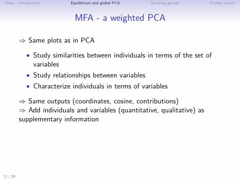
⇒ Same plots as in PCA

• Study similarities between individuals in terms of the set ofvariables

• Study relationships between variables• Characterize individuals in terms of variables

⇒ Same outputs (coordinates, cosine, contributions)⇒ Add individuals and variables (quantitative, qualitative) assupplementary information

11 / 39


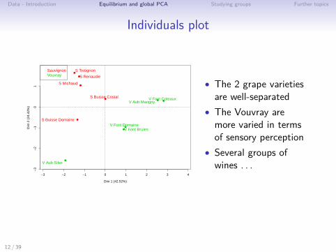
Individuals plot

●

−3 −2 −1 0 1 2 3 4

−3

−2

−1

01

Individual factor map

Dim 1 (42.52%)

Dim

2 (

24.4

2%)

S Michaud

S Renaudie

S Trotignon

S Buisse Domaine

S Buisse Cristal

V Aub Silex

V Aub Marigny

V Font Domaine V Font Brules

V Font Coteaux

●

●

●

●

●

●

●

●

●

●

SauvignonVouvray

• The 2 grape varietiesare well-separated

• The Vouvray aremore varied in termsof sensory perception

• Several groups ofwines . . .

12 / 39


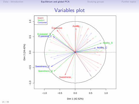
Variables plot

●

−1.5 −1.0 −0.5 0.0 0.5 1.0 1.5

−1.

0−

0.5

0.0

0.5

1.0

Correlation circle

Dim 1 (42.52%)

Dim

2 (

24.4

2%)

ExpertStudentConsumer

O.Intensity.before.shakingO.Intensity.after.shakingExpression

O.fruity

O.passion

O.citrus

O.candied.fruit

O.vanillaO.wooded

O.mushroom

O.plante

O.flower

O.alcohol

Typicity

Attack.intensity

Sweetness

Acidity

Bitterness

Astringency

Oxidation

Smoothness

Finesse

A.intensity

A.persistency

Visual.intensityGrade.colour

Surface.feeling

O.Intensity.before.shaking_S

O.Intensity.after.shaking_S

O.alcohol_SO.plante_S

O.mushroom_S

O.passion_S

O.Typicity_S A.intensity_S

Sweetness_S

Acidity_S

Bitterness_S

Astringency_S

A.alcohol_S

Balance_S

A.Typicity_S

O.Intensity.before.shaking_CO.Intensity.after.shaking_C

O.alcohol_C

O.plante_C

O.mushroom_C

O.passion_C

O.Typicity_C

A.intensity_C

Sweetness_C

Acidity_C

Bitterness_CAstringency_C

A.alcohol_C

Balance_CA.Typicity_C

13 / 39


Variables plot

●

−1.0 −0.5 0.0 0.5 1.0

−1.

0−

0.5

0.0

0.5

1.0

Correlation circle

Dim 1 (42.52%)

Dim

2 (

24.4

2%)


O.passion

Sweetness

Acidity

O.passion_S

Sweetness_S

Acidity_S

O.passion_C

Sweetness_C

Acidity_C

14 / 39


Outline





15 / 39


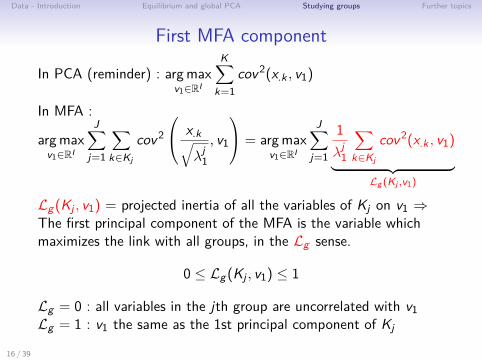
First MFA component

In PCA (reminder) : argmaxv1∈RI

K∑k=1

cov2(x.k , v1)

In MFA :

argmaxv1∈RI

J∑j=1

∑k∈Kj

cov2

x.k√λj1

, v1

= argmaxv1∈RI

J∑j=1

1λj1

∑k∈Kj

cov2(x.k , v1)

︸︷︷︸Lg (Kj ,v1)

Lg(Kj , v1) = projected inertia of all the variables of Kj on v1 ⇒The first principal component of the MFA is the variable whichmaximizes the link with all groups, in the Lg sense.

0 ≤ Lg(Kj , v1) ≤ 1

Lg = 0 : all variables in the jth group are uncorrelated with v1Lg = 1 : v1 the same as the 1st principal component of Kj

16 / 39


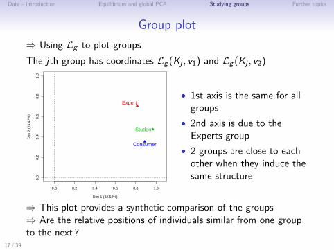
Group plot⇒ Using Lg to plot groupsThe jth group has coordinates Lg(Kj , v1) and Lg(Kj , v2)

●

0.0 0.2 0.4 0.6 0.8 1.0

0.0

0.2

0.4

0.6

0.8

1.0

Groups representation

Dim 1 (42.52%)

Dim

2 (

24.4

2%)

Expert

Student

Consumer

• 1st axis is the same for allgroups

• 2nd axis is due to theExperts group

• 2 groups are close to eachother when they induce thesame structure

⇒ This plot provides a synthetic comparison of the groups⇒ Are the relative positions of individuals similar from one groupto the next ?

17 / 39


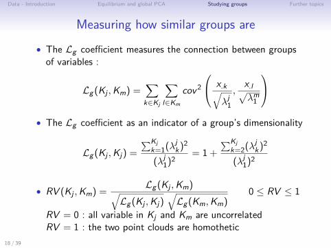
Measuring how similar groups are

• The Lg coefficient measures the connection between groupsof variables :

Lg(Kj ,Km) =∑k∈Kj

∑l∈Km

cov2

x.k√λj1

,x.l√λm1

• The Lg coefficient as an indicator of a group’s dimensionality

Lg(Kj ,Kj) =∑Kj

k=1(λjk)2

(λj1)2= 1 +

∑Kjk=2(λjk)2

(λj1)2

• RV (Kj ,Km) = Lg(Kj ,Km)√Lg(Kj ,Kj)

√Lg(Km,Km)

0 ≤ RV ≤ 1

RV = 0 : all variable in Kj and Km are uncorrelatedRV = 1 : the two point clouds are homothetic

18 / 39


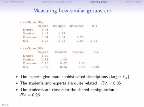
Measuring how similar groups are

> res$group$LgExpert Student Consumer MFA

Expert 1.45Student 1.17 1.29Consumer 0.94 1.04 1.25MFA 1.33 1.31 1.21 1.44

> res$group$RVExpert Student Consumer MFA

Expert 1.00Student 0.85 1.00Consumer 0.70 0.82 1.00MFA 0.92 0.96 0.90 1.00

• The experts give more sophisticated descriptions (larger Lg)• The students and experts are quite related : RV = 0.85• The students are closest to the shared configuration :

RV = 0.96

19 / 39


Partial points representation

⇒ Comparing groups in terms of individuals

⇒ Comparing descriptions provided by each group in a sharedspace

⇒ Are there specific individuals related to certain groups ofvariables ?

20 / 39


Projections of partial pointsxxxxxxxxxxxxxxxxxxxxxxxxxxxxxxxx

xxxxxxxxxxxxxxxxxxxxxxxx

xxxxxxxxxxxxxxxxxxxx

xxxxxxxxxxxxxxx


xxxxxxxxxxxxxxx

Data

Mean configuration of MFAG1 G2 G3

ii

21 / 39


Projections of partial pointsxxxxxxxxxxxxxxxxxxxxxxxxxxxxxxxx


xxxxxxxxxxxxxxxxxxxxxxxxxxxxxxxx


00000000000000000000000000000000

000000000000000000000000

00000000000000000000000000000000

000000000000000000000000


xxxxxxxxxxxxxxx


xxxxxxxxxxxxxxx


xxxxxxxxxxxxxxx


xxxxxxxxxxxxxxx

00000000000000000000

000000000000000

00000000000000000000

000000000000000

00000000000000000000

000000000000000

00000000000000000000

000000000000000

Projection of group 1



Data

Mean configuration of MFAG1 G2 G3

ii

i1

i2

i3

Mean point

Partial point 3

Partial point 2

Partial point 1

21 / 39


Partial points

What you expectedfor the tutorial

What you have learnedduring the tutorial

Tut

oria

l par

ticip

ants

F2

What you have learned during the tutorial

What you expected for the tutorial

What you have learnedduring the tutorial

What you expected for the tutorial

Disappointed or pleasantly surprised

Happy learner

F1

22 / 39


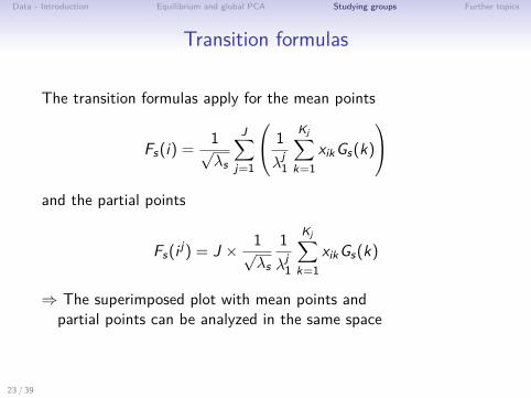
Transition formulas

The transition formulas apply for the mean points

Fs(i) = 1√λs

J∑j=1

1λj1

Kj∑k=1

xikGs(k)

and the partial points

Fs(i j) = J × 1√λs

1λj1

Kj∑k=1

xikGs(k)

⇒ The superimposed plot with mean points andpartial points can be analyzed in the same space

23 / 39


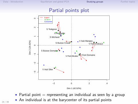
Partial points plot

●

−2 0 2 4

−3

−2

−1

01

23

Graph with the partial points

Dim 1 (42.52%)

Dim

2 (

24.4

2%)

●

●

●

●

●

●

●

●

●

●

●●

●●

●

●

●

●

●

●

●

●

●

●

●

●

●

●

●

●

S Michaud

S Renaudie

S Trotignon

S Buisse Domaine

S Buisse Cristal

V Aub Silex

V Aub Marigny

V Font Domaine V Font Brules

V Font Coteaux

●

●

●

●

●

●

●

●●

●


• Partial point = representing an individual as seen by a group• An individual is at the barycenter of its partial points24 / 39


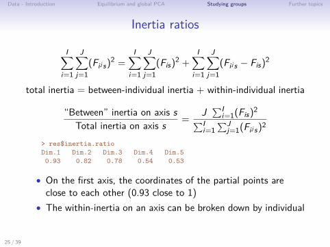
Inertia ratios

I∑i=1

J∑j=1

(Fi j s)2 =I∑

i=1

J∑j=1

(Fis)2 +I∑

i=1

J∑j=1

(Fi j s − Fis)2

total inertia = between-individual inertia + within-individual inertia

“Between” inertia on axis sTotal inertia on axis s = J

∑Ii=1(Fis)2∑I

i=1∑J

j=1(Fi j s)2

> res$inertia.ratioDim.1 Dim.2 Dim.3 Dim.4 Dim.50.93 0.82 0.78 0.54 0.53

• On the first axis, the coordinates of the partial points areclose to each other (0.93 close to 1)

• The within-inertia on an axis can be broken down by individual

25 / 39


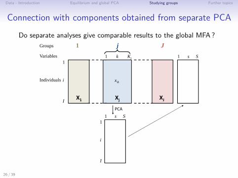
Connection with components obtained from separate PCA

Do separate analyses give comparable results to the global MFA ?

1

i

I

1

1 k Kj

xik

j J

X1 Xj XJ

PCA

1 s S1

i

I

Individuals

Variables

Groups

1 s S

26 / 39


Connection with components obtained from separate PCA

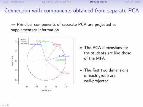
⇒ Principal components of separate PCA are projected assupplementary information

●

−1.0 −0.5 0.0 0.5 1.0

−1.

0−

0.5

0.0

0.5

1.0

Partial axes

Dim 1 (42.52%)

Dim

2 (

24.4

2%)

Dim1.Expert

Dim1.Student

Dim1.Consumer

Dim2.Expert

Dim2.Student

Dim2.Consumer


• The PCA dimensions forthe students are like thoseof the MFA

• The first two dimensionsof each group arewell-projected

27 / 39


Outline





28 / 39


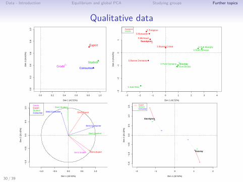
Qualitative data

• Balance the effect of each group of variables in the globalanalysis

• The usual plots for treating qualitative data (individuals andcategories)

• Specific plots (groups plot, superimposed plot, partial axesplots, separate analyses plots)

⇒ Same methodological approach, just replacing PCA with MCA

29 / 39


Qualitative data

●

0.0 0.2 0.4 0.6 0.8 1.0

0.0

0.2

0.4

0.6

0.8

1.0


Dim 1 (42.52%)

Dim

2 (

24.4

2%)

Expert

Student

ConsumerGrade

●

−3 −2 −1 0 1 2 3 4

−3

−2

−1

01


Dim 1 (42.52%)

Dim

2 (

24.4

2%)

S Michaud

S Renaudie

S Trotignon

S Buisse Domaine

S Buisse Cristal

V Aub Silex

V Aub Marigny

V Font Domaine V Font Brûlés

V Font Coteaux

Sauvignon

Vouvray

●

●

●

●

●

●

●

●

●

●

SauvignonVouvray

●

−1.0 −0.5 0.0 0.5 1.0

−1.

0−

0.5

0.0

0.5

1.0

Partial axes

Dim 1 (42.52%)

Dim

2 (

24.4

2%)

Dim1.Expert

Dim2.Student

Dim1.Student

Dim1.Consumer

Dim2.Expert

Dim1.Grade

Dim2.Consumer

GradeExpertStudentConsumer

●

−2 −1 0 1 2

−1.

5−

1.0

−0.

50.

00.

51.

01.

5


Dim 1 (42.52%)

Dim

2 (

24.4

2%)

Sauvignon

Vouvray


30 / 39


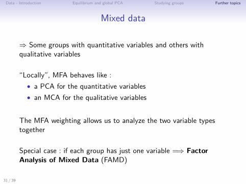
Mixed data

⇒ Some groups with quantitative variables and others withqualitative variables

“Locally”, MFA behaves like :• a PCA for the quantitative variables• an MCA for the qualitative variables

The MFA weighting allows us to analyze the two variable typestogether

Special case : if each group has just one variable =⇒ FactorAnalysis of Mixed Data (FAMD)

31 / 39


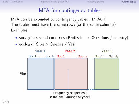
MFA for contingency tablesMFA can be extended to contingency tables : MFACTThe tables must have the same rows (or the same columns)Examples

• survey in several countries (Profession × Questions / country)• ecology : Sites × Species / Year

Site

Spe 1 . . . Spe J1 Spe 1 . . . Spe J2 Spe 1 . . . Spe JK

Year 1 Year 2 Year K

Frequency of species jin the site i during the year 2

32 / 39


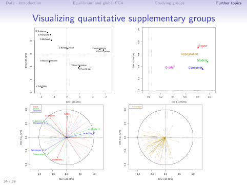
Plotting supplementary information

Expert(27)

Student(15)

Consumer(15)

Appreciation(60)

Grapevariety

(1)

Wine 1

Wine 2

…

Wine 10

Questions :

• Are preferences linked with sensory characteristics ?• Does the grape variety explain the sensory characteristics ?

33 / 39


Visualizing quantitative supplementary groups

●

−2 −1 0 1 2 3

−3

−2

−1

01


Dim 1 (42.52%)

Dim

2 (

24.4

2%)

S Michaud

S Renaudie

S Trotignon

S Buisse Domaine

S Buisse Cristal

V Aub Silex

V Aub Marigny

V Font Domaine

V Font Brûlés

V Font Coteaux

●

●

●

●

●

●

●

●

●

●

●

0.0 0.2 0.4 0.6 0.8 1.0

0.0

0.2

0.4

0.6

0.8

1.0


Dim 1 (42.52%)

Dim

2 (

24.4

2%)

Expert

Student

ConsumerGrade

Appreciation

●

−1.0 −0.5 0.0 0.5 1.0

−1.

0−

0.5

0.0

0.5

1.0

Correlation circle

Dim 1 (42.52%)

Dim

2 (

24.4

2%)


O.passion

Sweetness

Acidity

O.passion_S

Sweetness_S

Acidity_S

O.passion_C

Sweetness_C

Acidity_C

●

−1.0 −0.5 0.0 0.5 1.0

−1.

0−

0.5

0.0

0.5

1.0

Correlation circle

Dim 1 (42.52%)

Dim

2 (

24.4

2%)

Appreciation

34 / 39


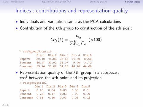
Indices : contributions and representation quality

• Individuals and variables : same as the PCA calculations• Contribution of the kth group to construction of the sth axis :

Ctrs(k) = Fks∑Kk=1 Fks

(×100)

> res$group$contribDim.1 Dim.2 Dim.3 Dim.4 Dim.5

Expert 30.49 45.99 33.68 44.59 40.60Student 36.27 30.92 35.07 9.20 14.72Consumer 33.24 23.09 31.25 46.20 44.68

• Representation quality of the kth group in a subspace :cos2 between the kth point and its projection> res$group$cos2

Dim.1 Dim.2 Dim.3 Dim.4 Dim.5Expert 0.46 0.34 0.03 0.03 0.01Student 0.73 0.17 0.03 0.00 0.00Consumer 0.63 0.10 0.03 0.03 0.02

35 / 39


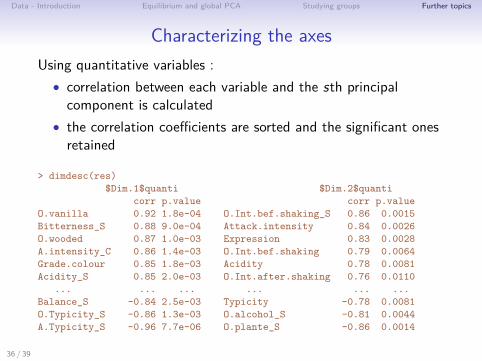
Characterizing the axesUsing quantitative variables :

• correlation between each variable and the sth principalcomponent is calculated

• the correlation coefficients are sorted and the significant onesretained

> dimdesc(res)$Dim.1$quanti $Dim.2$quanti

corr p.value corr p.valueO.vanilla 0.92 1.8e-04 O.Int.bef.shaking_S 0.86 0.0015Bitterness_S 0.88 9.0e-04 Attack.intensity 0.84 0.0026O.wooded 0.87 1.0e-03 Expression 0.83 0.0028A.intensity_C 0.86 1.4e-03 O.Int.bef.shaking 0.79 0.0064Grade.colour 0.85 1.8e-03 Acidity 0.78 0.0081Acidity_S 0.85 2.0e-03 O.Int.after.shaking 0.76 0.0110

... ... ... ... ... ...Balance_S -0.84 2.5e-03 Typicity -0.78 0.0081O.Typicity_S -0.86 1.3e-03 O.alcohol_S -0.81 0.0044A.Typicity_S -0.96 7.7e-06 O.plante_S -0.86 0.0014

36 / 39


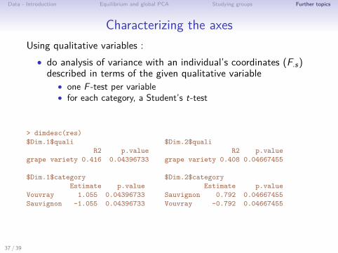
Characterizing the axesUsing qualitative variables :

• do analysis of variance with an individual’s coordinates (F.s)described in terms of the given qualitative variable

• one F -test per variable• for each category, a Student’s t-test

> dimdesc(res)$Dim.1$quali $Dim.2$quali

R2 p.value R2 p.valuegrape variety 0.416 0.04396733 grape variety 0.408 0.04667455

$Dim.1$category $Dim.2$categoryEstimate p.value Estimate p.value

Vouvray 1.055 0.04396733 Sauvignon 0.792 0.04667455Sauvignon -1.055 0.04396733 Vouvray -0.792 0.04667455

37 / 39


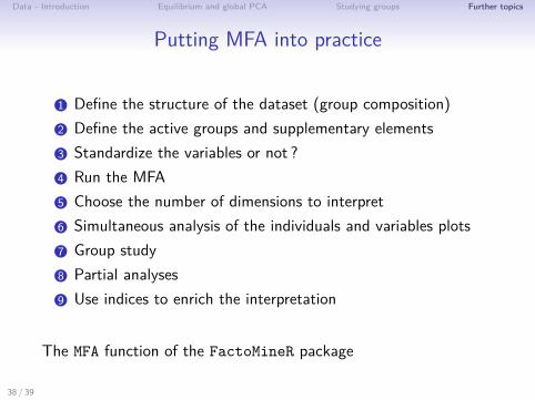
Putting MFA into practice

1 Define the structure of the dataset (group composition)2 Define the active groups and supplementary elements3 Standardize the variables or not ?4 Run the MFA5 Choose the number of dimensions to interpret6 Simultaneous analysis of the individuals and variables plots7 Group study8 Partial analyses9 Use indices to enrich the interpretation

The MFA function of the FactoMineR package

38 / 39


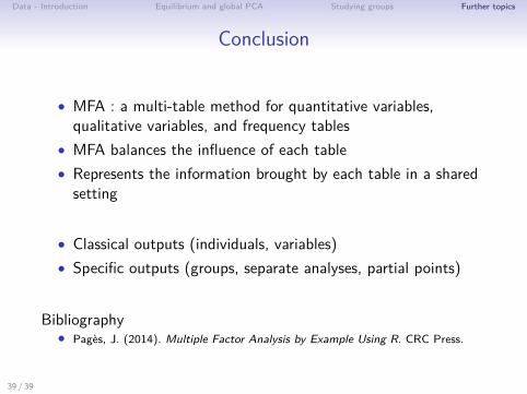
Conclusion

• MFA : a multi-table method for quantitative variables,qualitative variables, and frequency tables

• MFA balances the influence of each table• Represents the information brought by each table in a sharedsetting

• Classical outputs (individuals, variables)• Specific outputs (groups, separate analyses, partial points)

Bibliography• Pagès, J. (2014). Multiple Factor Analysis by Example Using R. CRC Press.

39 / 39

Documents

Multiple Factor Analysis - Freefactominer.free.fr/course/doc/MFA_course_slides.pdfMultiple Factor Analysis ... IntroductionEquilibrium and global PCAStudying groupsFurther topics