Multiple crossdocks with inventory and time windowsguoys/publications/CORCrossDock_Guo.pdf · Crossdocking studies have mostly been concerned with the physical layout of a crossdock

Computers & Operations Research 33 (2006) 43–63

www.elsevier.com/locate/cor

Multiple crossdocks with inventory and time windows

Ping Chena, Yunsong Guob, Andrew Limc, Brian Rodriguesd,∗aDepartment of Computer Science, University of Maryland, College Park, MD 20742, USA

bDepartment of Computer Science, National University of Singapore, 3 Science Drive 2, Singapore 117543, SingaporecDepartment of IEEM, Hong Kong University of Science and Technology, Clear Water Bay, Hong Kong

dSchool of Business, Singapore Management University, 469 Bukit Timah Road, Singapore 259756, Singapore

Available online 23 August 2004

Abstract

Crossdocking studies have mostly been concerned with the physical layout of a crossdock or on a single cross-dock. In this work, we study a network of crossdocks taking into consideration delivery and pickup time windows,warehouse capacities and inventory-handling costs. Because of the complexity of the problem, local search tech-niques are developed and used with simulated annealing and tabu search heuristics. Extensive experiments wereconducted and results show that the heuristics outperform CPLEX, providing solutions in realistic timescales.� 2004 Elsevier Ltd. All rights reserved.

Keywords:Crossdocking; JIT; Heuristics

1. Introduction

The “just-in-time” (JIT) inventory management (orkanban) principle requires that there is just enoughinventory that arrives to replace what has been used.As a result, warehousing large inventories has becomeless common, and can be, in some situations, detrimental to business. The implementation of crossdockoperations repositions the focus from warehousing inventory to one of managing inventory through-flowin transit from suppliers to customers. In this process, the warehouses, as crossdocks, are transformedfrom inventory repositories to points of delivery, consolidation and pickup. Advantages of crossdockingcan accrue from the reduction of warehousing costs, inventory-holding costs, service cycle times andtransportation costs.

∗ Corresponding author. Tel.: +65-68220709; fax: +65-68220777.E-mail address:[email protected](B. Rodrigues).

0305-0548/$ - see front matter� 2004 Elsevier Ltd. All rights reserved.doi:10.1016/j.cor.2004.06.002

http://www.elsevier.com/locate/cor

mailto:[email protected]

44 P. Chen et al. / Computers & Operations Research 33 (2006) 43–63

The use of “crossdocking” has become synonymous with rapid consolidation and processing.Napolitano[1] proposed a scheme which describes the various types of crossdocking operations. Theseinclude manufacturing, distributor, transportation, retail and opportunistic crossdocking. Inthese, a common feature is consolidation and short cycle times, of usually less than aday[2].

Napolitano[1] also describes crossdocking as the “JIT in the distribution arena”. In the manufactur-ing area, crossdocking constitutes the receiving and consolidating of inbound supplies where a man-ufacturer can use a warehouse to receive supplies of parts for demands ascertained from an MRP. Inretail crossdocking, retailers receive products from multiple vendors who use distributors with mul-tiple warehouses. In general, crossdocks are complex, requiring a high degree of coordination be-tween suppliers, customers and distributors to create shipments based on anticipated supplies and de-mands[3]. In all crossdocking situations, the timing of delivery and pickup is crucial to effectiveoperations.

A significant amount of work on crossdocking has focused on the crossdock itself. In[4], Bartholdiand Gue determined the best shape for a crossdock analyzing the assignment of receiving and shippingdoors. The staging of products in a crossdock to avoid floor congestion and increase throughput has alsobeen studied together with the effects of different combinations of number of workers in receiving andshipping on throughput[2,5,6]. In [7], a simulated annealing procedure was used to construct effectivelayout to reduce labor costs. Other studies have treated crossdocks as a network of distribution and/ortransshipment points. Donaldson et al.[8] studies a schedule-driven mail transportation in US and Ratliffet al.[9] studied a load-driven network, in which deliveries take place when there are sufficient productswaiting for transportation. Donaldson et al.[8] studied a network of crossdocks for the US Postal Servicewhere 148Area Distribution Centers serve as crossdocks, each receiving, sorting, packing and dispatchingmail according to operating schedules. Mail not processed on time must be shipped by air, incurringadditional costs and “critical-entry” times, when mail must arrive at the destination center, must becoordinated with transportation schedules to avoid overshooting specified cutoff times. Each distributioncenter serves as an origin as well as destination node where schedules were driven by mail deliverystandards. Ratliff et al.[9] studied the NorthAmerican automobile delivery systems to determine the idealnumber and location of crossdocks in a network and how shipments flowed between them. In their study, aminimum inventory strategy was key in attempting to minimize the number of vehicles at the mixing center(crossdocks).

Crossdocking can be complex and difficult to manage, involving a large number of transshipmentpoints and vehicles. The well-known success of Wal Mart[10] in crossdocking requires coordinat-ing 2000 dedicated trucks over a large network of warehouses, crossdocks and retail points. Maytag,a large distributor of household appliances maintains 41 crossdock facilities where “no inventory isheld” [11].

One benefit arising from crossdocking is reduced handling costs at a company’s facility because itminimizes “the number of touches”[12]. In addition, when timing is well coordinated, a product can bemade available in shorter time windows, thus reducing cycle times. Although central to crossdocking,studies found in the literature have not taken handling costs and delivery and time considerations intoaccount. Further work has mostly focused on a single crossdock. In this work, we extend the work ofDonaldson et al.[8] and Ratcliff et al.[9], in studying crossdocking networks. In particular, we studycrossdocking scheduling where time windows for deliveries and pickups are considered.Also, we considercrossdock-handling costs which are use to penalize delays. Although we study the occurrence of multiple

P. Chen et al. / Computers & Operations Research 33 (2006) 43–63 45

transshipment points, the model proposed can be used for a single transshipment point, where timewindow constraints, inventory-handing costs and warehouse capacity are relevant, as, for example, formanufacturing crossdocking where the JIT-driven manufacturer uses a single warehouse to receive anddeliver subassemblies and parts.

2. The multiple crossdock problem

2.1. Background

The crossdocking problem is closely related to the minimum-cost multicommodity flow problem(MCMFP) and the transshipment problem. It is therefore worthwhile to distinguish between the problemshere. Although both problems involve finding minimum cost multicommodity flow, the crossdockingproblem differs from the MCMFP as there is no explicit source and sink pair for each commodityand the total supply and demand of each commodity need not be equal. Another difference is that thequantity specified by a single delivery or pickup cannot be split during the distribution process. Further,the relationship between deliveries and pickups is many-to-many and for a matched pair of deliveryand pickup, there is in many cases only one crossdock which works as a transshipment point betweenthem. In the MCMFP, any node other than source and destination nodes can be used as transshipmentpoints.

The transshipment problem consists of a number of supply, transshipment and demand nodes. Dif-ferent capacity limits and costs are assigned to arcs between nodes. As in the MCMFP, the objec-tive is to find a minimum cost flow that meets all demands and the capacity constraints. The prob-lem deals with a single commodity but allows multiple sources and sinks, which distinguishes it fromthe MCMFP. Further, properties such as non-splitable deliveries and pickups, time window considera-tions and storage allowed on crossdocks distinguish the crossdocking problem from the transshipmentproblem.

2.2. Problem description

As described, the objective in crossdocking problem is to find a minimum cost distribution plan in-volving crossdocks based on anticipated supplies and demands. Supplies and demands are taken asdeliveries and pickups within time windows. For delivery, we use(s, p, amount, [st, et]) to mean thatsuppliers can supply quantityamountof productp in the time window[st, et]. For pickup,c replacess, wherec is the customer who picks up the product. Each crossdocki has a capacity(CAP i), whichis the maximum inventory it can hold at any time, and an inventory-handling cost(COST i), measuredon a per unit product and per unit time basis. As crossdocks can vary in their handling capabilities,the latter cost is dependent on the particular crossdock. This cost is key to the model we proposesince it penalizes delays at crossdocks so that shipments can be, as far as possible, transferred fromincoming to outgoing trailers with little or no storage in between. In most cases, this cost is small com-pared to transportation costs. We takeC to be a set of crossdocks,D to denote a set of deliveries andP to be a set of pickups, and assume that: (1) all demands must be met, (2) the time window con-straint of each fulfilled delivery and each pickup must not be violated, (3) the inventory level of each


crossdock cannot exceed its capacity at all times, and (4) flow conservation holds for all products at alltimes.

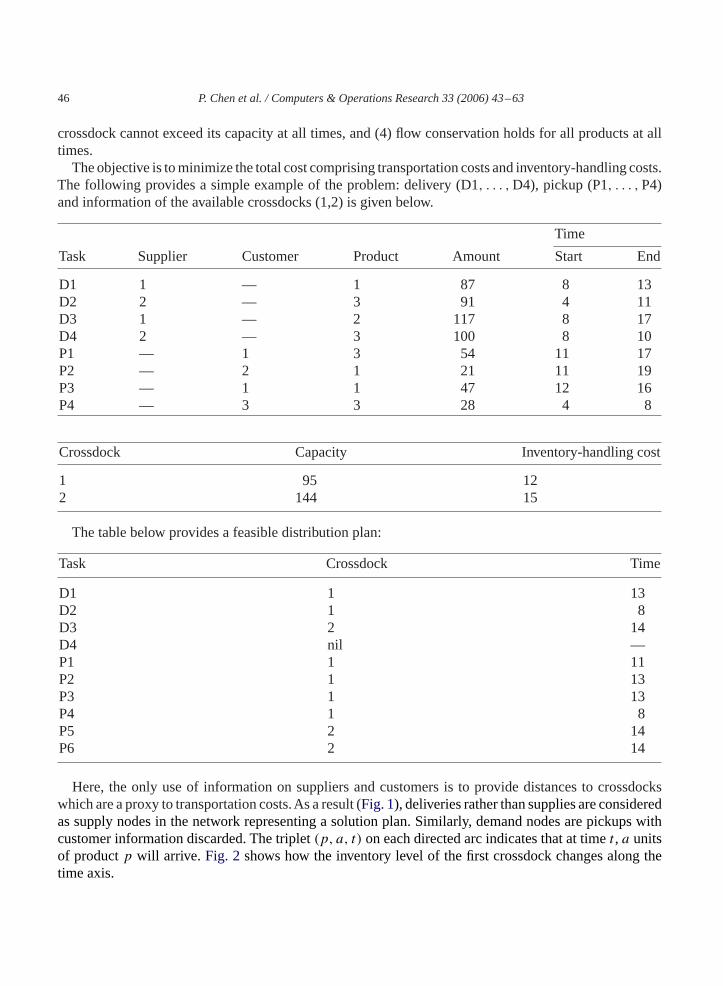
The objective is to minimize the total cost comprising transportation costs and inventory-handling costs.The following provides a simple example of the problem: delivery (D1, . . . ,D4), pickup (P1, . . . ,P4)and information of the available crossdocks (1,2) is given below.

Time

Task Supplier Customer Product Amount Start End

D1 1 — 1 87 8 13D2 2 — 3 91 4 11D3 1 — 2 117 8 17D4 2 — 3 100 8 10P1 — 1 3 54 11 17P2 — 2 1 21 11 19P3 — 1 1 47 12 16P4 — 3 3 28 4 8

Crossdock Capacity Inventory-handling cost

1 95 122 144 15

The table below provides a feasible distribution plan:

Task Crossdock Time

D1 1 13D2 1 8D3 2 14D4 nil —P1 1 11P2 1 13P3 1 13P4 1 8P5 2 14P6 2 14

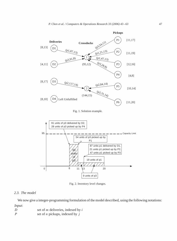
Here, the only use of information on suppliers and customers is to provide distances to crossdockswhich are a proxy to transportation costs.As a result (Fig. 1), deliveries rather than supplies are consideredas supply nodes in the network representing a solution plan. Similarly, demand nodes are pickups withcustomer information discarded. The triplet(p, a, t) on each directed arc indicates that at timet , a unitsof productp will arrive. Fig. 2 shows how the inventory level of the first crossdock changes along thetime axis.


1

2

D1

D2

D3

P6

P5

P4

P3

P2

P1

(p1,87,13)

(p3,91,8)

(p2,117,14)

(p3,54,11)

(p1,21,13)

(p1,47,13)(p3,28,8)

(p2,84,14)

(p2,31,14)

(95,12)

(144,15)

Deliveries

Pickups

D4

Crossdocks

Left Unfulfilled

[8,13]

[4,11]

[8,17]

[8,10][11,20]

[10,14]

[4,8]

[12,16]

[11,19]

[11,17]

Fig. 1. Solution example.

63units

ofp3

8 11 13 200

95

91 units of p3 delivered by D2,28 units of p3 picked up by P4

54 units of p3 picked up byP1

87 units p1 delivered by D1,21 units p1 picked up by P2,47 units p1 picked up by P3

9 units of p3

19 units of p1

Capacity Limit

Fig. 2. Inventory level changes.

2.3. The model

We now give a integer-programming formulation of the model described, using the following notations:

Input:D set ofm deliveries, indexed byiP set ofn pickups, indexed byj


C set ofc crossdocks, indexed bykG set ofd products, indexed byrT set of times, indexed byt

Parameters:DP binary incidence matrix, whereDP i,r is 1 if productr is delivered by deliveryi, and 0

otherwiseDA vector whereDAi is the amount delivered by deliveryiDD matrix whereDDi,k is the distance from deliveryi to crossdockkDS vector whereDSi is starting time of deliveryiDE vector whereDEi is the ending time of deliveryi with pickup parameters

PP ,PA,PD,PS, PE defined similarlyCAP vector whereCAPk is the capacity of crossdockkCOST vector whereCOST k is the cost of handling a unit product for a unit time at crossdockk

Tmin, Tmax minimum and maximum times defining the time horizon

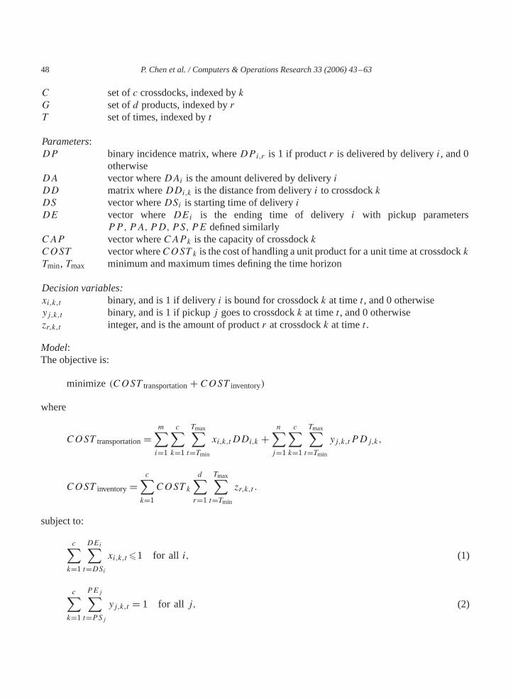
Decision variables:xi,k,t binary, and is 1 if deliveryi is bound for crossdockk at timet , and 0 otherwiseyj,k,t binary, and is 1 if pickupj goes to crossdockk at timet , and 0 otherwisezr,k,t integer, and is the amount of productr at crossdockk at timet .

Model:The objective is:

minimize (COST transportation+ COST inventory)

where

COST transportation=m∑

i=1

c∑

k=1

Tmax∑

t=Tmin

xi,k,tDDi,k +n∑

j=1

c∑

k=1

Tmax∑

t=Tmin

yj,k,tPDj,k,

COST inventory=c∑

k=1

COST k

d∑

r=1

Tmax∑

t=Tmin

zr,k,t .

subject to:

c∑

k=1

DEi∑

t=DSixi,k,t �1 for all i, (1)

c∑

k=1

PEj∑

t=PSjyj,k,t = 1 for all j, (2)


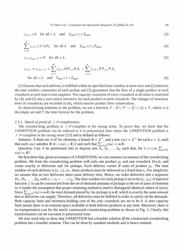
zr,k,t �0 for all r, k and Tmin� t�Tmax, (3)

d∑

r=1

zr,k,t �CAPk for all k and Tmin� t�Tmax, (4)

zr,k,Tmin−1= 0 for all r, k, (5)

zr,k,t = zr,k,t−1+m∑

i=1

xi,k,tDP i,rDAi −n∑

j=1

yj,k,tPP j,rPAj

for all r, k and Tmin� t�Tmax. (6)

(1) Ensures that each delivery is fulfilled within its specified time window at most once and (2) enforcesthe time window constraints of each pickup and (3) guarantees that the flow of a single product at eachcrossdock at each time is non-negative. The capacity constraint of every crossdock at all times is restrictedby (4), and (5) sets a zero initial inventory for each product at each crossdock. The changes of inventorylevel of crossdocks are recorded in (6), which ensures product flow conservation.

In characterizing solutions to the problem, we use a functionF : D ∪ P → [C ∪ �] × T , where� isthe empty set andT the time horizon for the problem.

2.3.1. Sketch of proof ofNP-completenessThe crossdocking problem isNP-complete in the strong sense. To prove this, we show that the

3-PARTITION problem can be reduced to it in polynomial time where the 3-PARTITION problem isNP-complete in the strong sense[13] and is defined as follows:Instance:A finite setA of 3m elements, a boundB ∈ Z+, and a sizes(a) ∈ Z+ for eacha ∈ A, such

that eachs(a) satisfiesB/4<s(a)<B/2 and such that∑

a∈As(a)=mB.Question:CanA be partitioned intom disjoint setsS1, S2, . . . , Sm such that, for 1�i�m,

∑a∈Si

s(a)= B?We first show that, given an instance of 3-PARTITION, we can construct an instance of the crossdocking

problem. We form the crossdocking problem with only one productp1 and one crossdockDock1 andcreate exactlym deliveries and 3m pickups. Each delivery carriesB units of productp1. The timewindow of each delivery is[ti , ti], i.e., those products must be delivered at a fixed timeti . For simplicity,we assume that no two deliveries share same delivery time. Hence, we order deliveries into a sequenceD1,D2, . . . , Dm with t1< t2< · · ·< tm. The time window for each pickup is set to be[t1, tm]. A bijectivefunctionf is can be constructed from the set of demand amounts of pickups to the set of sizes of elementsin A (under the assumption that proper renaming method is used to distinguish identical values of sizes).Since

∑a∈As(a)=mB, the total demand placed by 3m pickups ismB, which is exactly the same amount

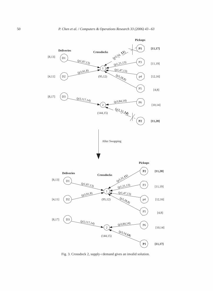
thatm deliveries can supply. Therefore, all deliveries must be fulfilled in order to satisfy all the demands.Both capacity limit and inventory-holding cost of the only crossdock are set to be 0. A zero capacitylimit means there is no external space available to hold leftover products at any time. Moreover, there isno transportation cost for the newly constructed crossdocking problem as shown inFig. 3. Clearly, thistransformation can be executed in polynomial time.

We now need only to show that 3-PARTITION has a feasible solutioniff the constructed crossdockingproblem has a feasible solution. This can be done by standard methods and is hence omitted.


1

2

D1

D2

D3

P2

P6

P5

p4

P3

P1

(p1,87,13)

(p3,91,8)

(p3,117,14)

(p3,54,11)

(p1,21,13)

(p1,47,13)(p3,28,8)

(p3,84,14)

(p3,31,14)

(95,12)

(144,15)

Deliveries

Pickups

Crossdocks

[8,13]

[4,11]

[8,17]

[11,20]

[10,14]

[4,8]

[12,16]

[11,19]

[11,17]

1

2

D1

D2

D3

P1

P6

P5

p4

P3

P2

(p1,87,13)

(p3,91,8)

(p3,117,14)

(p3,31,11)

(p1,21,13)

(p1,47,13)(p3,28,8)

(p3,84,14)

(p3,54,14)

(95,12)

(144,15)

Deliveries

Pickups

Crossdocks

[8,13]

[4,11]

[8,17]

[11,17]

[10,14]

[4,8]

[12,16]

[11,19]

[11,20]

After Swapping

Fig. 3. Crossdock 2, supply<demand gives an invalid solution.


3. Initial solutions

Although using integer programming (IP) can lead to good results, IP methods can fail for large-sizeproblems. In view of the complexity of the crossdocking problem, our approach was therefore to first uselocal search techniques.

For each delivery and pickup, we need only determine the values of two decision variables: the choiceof the crossdock and the time of delivery or pickup. Simple methods such as randomly assigning valuesnormally fail to produce feasible solutions in view of the difficult constraints present. We therefore use agreedy method to obtain initial solutions.

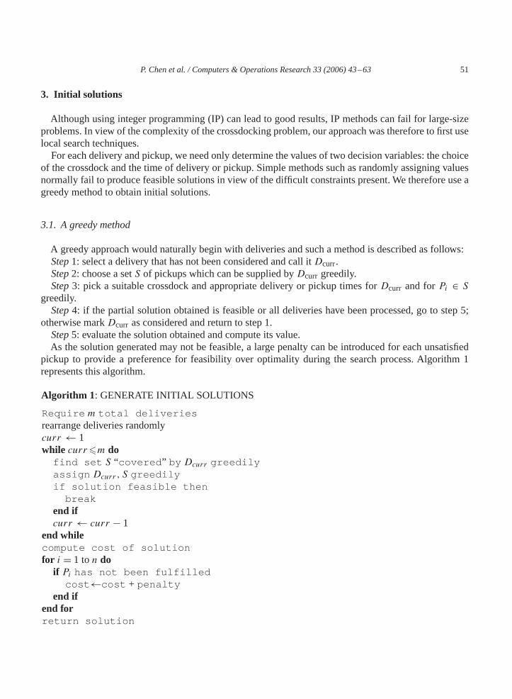
3.1. A greedy method

A greedy approach would naturally begin with deliveries and such a method is described as follows:Step1: select a delivery that has not been considered and call itDcurr.Step2: choose a setS of pickups which can be supplied byDcurr greedily.Step3: pick a suitable crossdock and appropriate delivery or pickup times forDcurr and forPi ∈ S

greedily.Step4: if the partial solution obtained is feasible or all deliveries have been processed, go to step 5;

otherwise markDcurr as considered and return to step 1.Step5: evaluate the solution obtained and compute its value.As the solution generated may not be feasible, a large penalty can be introduced for each unsatisfied

pickup to provide a preference for feasibility over optimality during the search process. Algorithm 1represents this algorithm.

Algorithm 1 : GENERATE INITIAL SOLUTIONS

Require m total deliveriesrearrange deliveries randomlycurr ← 1while curr�m do

find set S “covered ” by Dcurr greedilyassign Dcurr , S greedilyif solution feasible then

breakend ifcurr ← curr − 1

end whilecompute cost of solutionfor i = 1 ton do

if Pi has not been fulfilledcost ←cost + penalty

end ifend forreturn solution


Given a deliveryDcurr = (p, a, [s, e]), a set of pickupsS = {Pi |Pi = (pi, ai, [si, ei])} is said to be“covered” byDcurr if it satisfies the following conditions:

1. for allPi ∈ S, pi = p2. for allPi ∈ S,

∑ai�a

3. for allPi ∈ S, ei�s.

In the algorithm above, we need to find such anS. Conditions 1 and 2 are clear. Condition 3 ensuresthat in order forDcurr to “cover” all pickups inS, it must be available before the latest demand time ofeach pickup. To find such a “covered” setS, two greedy methods can be used:First Fit andBestFit . As the name suggests, theFirst Fit greedy method attempts to find the first set that meets allcriteria. On the other hand,Best Fit aims to find the best set, where a set is “best” if|a −∑

ai | isminimized so that inventories to be stocked are reduced to the lowest possible level. Finding the best setcan be achieved in pseudo-polynomial time using a dynamic programming method[14].

To assignDcurr andS in the algorithm, we note that determining crossdocks and times forDcurr andeachPi ∈ S is a tedious task as the validity of partial solutions needs to be maintained at all times. Ageneral strategy, used to determine time, is to deliver as late as possible and to pick up as early as possiblein order to reduce potential inventory-holdings levels. For crossdocks, decisions are made by choosing thefirst fit crossdock. Depending on the crossdocks, we approach such assignments in a loose or tight way.The “loose” approach looks for crossdocks with space larger than required, ignoring that pickups canoccur at the same time. On the other hand, a “tight” approach takes the latter into account, and considersavailable space at all times. The “tight” approach is employed in theBest Fit greedy method, whilethe “loose” approach is used in theFirst Fit method.

4. Heuristics

In this section, we will introduce our heuristic methods by providing the design of neighborhood movesand the construction of our simulated annealing, tabu search and a hybrid heuristic methods.

4.1. Neighborhood search

A basic component of any local search is neighborhood search. A solutions′ is said to be a neighbor ofanother solutions if it can be obtained froms through a neigborhood move. We developed a number ofsuch moves suitable for this problem which we use in the heuristics developed here to find neigborhoodsolutions. These moves are key to the successful implementation of these heuristics.Swap two pickups: First, randomly select two pickups which demand the same productp: P1 =

(p, a1, [s1, e1]) andP2= (p, a2, [s2, e2]). Suppose in solutions, F(P1)= (d1, t1) andF(P2)= (d2, t2)

with d1 �= d2, which means that the product is bound for different crossdocks. If ad1 or d2 is actuallya dummy crossdock, then the corresponding pickup has not been fulfilled. In this case, swapping is infact a replacement of one fulfilled pickup with an unfulfilled one. Swapping pickups can be as simple asexchanging cross-docks and the times assigned to them. Therefore, in the new solutions′,F ′(P1)=(d2, t2)

andF ′(P2)=(d1, t1)withF ′(Pi)=F(Pi) if i /∈ {1,2}. If the new crossdock assigned is actually a dummy,


the time mapped underF ′must be set to 0 to be consistent. This move is valid only if the resultant solutions′ is valid. Fig. 3 shows how such a swap can be achieved.

However, the following problems can arise due to constraints placed on time windows, flow conser-vation, inventory level limits, etc.: (1) the new time does not fit its time window, (2) the inventory levelexceeds the limit atd1 or d2 or both, (3) the flow conservation rule of productp is violated atd1 or d2 orboth.

The first case can be resolved by adjusting the invalid time to the nearest feasible time within itsrange. The adjustment of time is indeed either postponing or predating pickups, thus inventory levelsof affected crossdocks should be kept updated consistently. The latter two cases of inventory-relatedconstraints violation may occur after adjustment. Proper repair procedures dealing with inventories haveto be defined in order to ensure validity of the new solution.

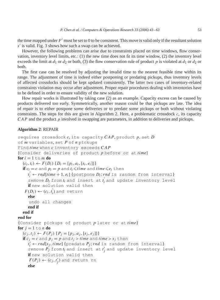
How repair works is illustrated by taking case (2) as an example. Capacity excess can be caused byproducts delivered too early. Symmetrically, another reason could be that pickups are late. The ideaof repair is to either postpone some deliveries or to predate some pickups or both without violatingconstraints. The steps for this are given in Algorithm 2. Here, a problematic crossdockc, its capacityCAP and the productp involved in swapping are parameters, in addition to deliveries and pickups.

Algorithm 2 : REPAIR

requires crossdock c, its capacity CAP , product p, set D

of m variables , set P of n pickupsFind t ime when c inventory exceeds CAP

{Consider deliveries of product p before or at t ime}for i = 1 to m do(ci, ti)← F(Di) {Di = {pi, ai, [si, ei]}}if ci = c and pi = p and ti� t ime and t ime�ei then

t′i ← rnd[t ime + 1, ei] { postpone Di; rnd is random from interval }

remove Di from ti and insert at t′i and update inventory level

if new solution valid then

F(Di)← (ci, t′i ) and return

elseundo all changesend if

end ifend for{ Consider pickups of product p later or at t ime}for j = 1 to n do(cj , tj )← F(Pj ) {Pj = {pj , aj , [sj , ej ]}}if cj = c and pj = p and tj > time and t ime> sj thent ′i ← rnd[sj , time] { predate Pj ; rnd is random from interval }remove Pj from ti and insert at t ′j and update inventory levelif new solution valid thenF(Pj )← (cj , t

′j ) and return rn

else


undo all changesend if

end ifend for

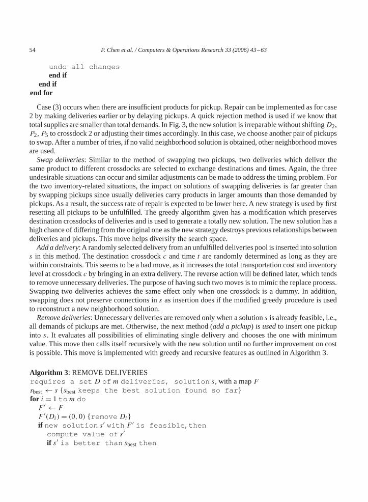
Case (3) occurs when there are insufficient products for pickup. Repair can be implemented as for case2 by making deliveries earlier or by delaying pickups. A quick rejection method is used if we know thattotal supplies are smaller than total demands. In Fig. 3, the new solution is irreparable without shiftingD2,P2,P5 to crossdock 2 or adjusting their times accordingly. In this case, we choose another pair of pickupsto swap. After a number of tries, if no valid neighborhood solution is obtained, other neighborhood movesare used.Swap deliveries: Similar to the method of swapping two pickups, two deliveries which deliver the

same product to different crossdocks are selected to exchange destinations and times. Again, the threeundesirable situations can occur and similar adjustments can be made to address the timing problem. Forthe two inventory-related situations, the impact on solutions of swapping deliveries is far greater thanby swapping pickups since usually deliveries carry products in larger amounts than those demanded bypickups. As a result, the success rate of repair is expected to be lower here. A new strategy is used by firstresetting all pickups to be unfulfilled. The greedy algorithm given has a modification which preservesdestination crossdocks of deliveries and is used to generate a totally new solution. The new solution has ahigh chance of differing from the original one as the new strategy destroys previous relationships betweendeliveries and pickups. This move helps diversify the search space.Add a delivery:A randomly selected delivery from an unfulfilled deliveries pool is inserted into solution

s in this method. The destination crossdockc and timet are randomly determined as long as they arewithin constraints. This seems to be a bad move, as it increases the total transportation cost and inventorylevel at crossdockc by bringing in an extra delivery. The reverse action will be defined later, which tendsto remove unnecessary deliveries. The purpose of having such two moves is to mimic the replace process.Swapping two deliveries achieves the same effect only when one crossdock is a dummy. In addition,swapping does not preserve connections ins as insertion does if the modified greedy procedure is usedto reconstruct a new neighborhood solution.Remove deliveries: Unnecessary deliveries are removed only when a solutions is already feasible, i.e.,

all demands of pickups are met. Otherwise, the next method (add a pickup) is usedto insert one pickupinto s. It evaluates all possibilities of eliminating single delivery and chooses the one with minimumvalue. This move then calls itself recursively with the new solution until no further improvement on costis possible. This move is implemented with greedy and recursive features as outlined in Algorithm 3.

Algorithm 3 : REMOVE DELIVERIESrequires a set D of m deliveries, solution s, with a mapFsbest← s { sbestkeeps the best solution found so far }for i = 1 to m doF ′ ← F

F ′(Di)= (0,0) { remove Di}if new solution s′ with F ′ is feasible , then

compute value of s′if s′ is better than sbest then


sbest← s′end if

end ifend forif sbest is better than s′ then

call REMOVEwith solution sbestelse

returnend if

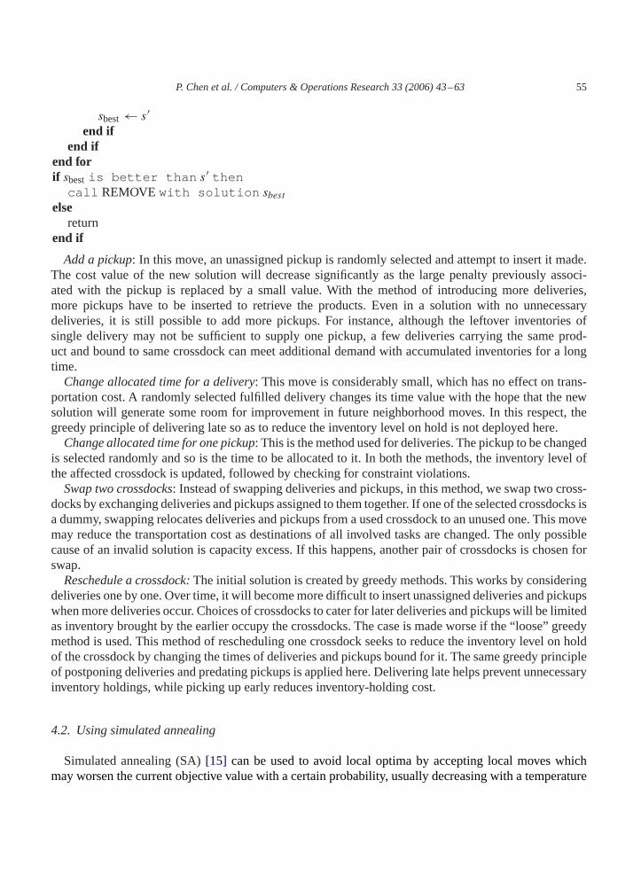
Add a pickup: In this move, an unassigned pickup is randomly selected and attempt to insert it made.The cost value of the new solution will decrease significantly as the large penalty previously associ-ated with the pickup is replaced by a small value. With the method of introducing more deliveries,more pickups have to be inserted to retrieve the products. Even in a solution with no unnecessarydeliveries, it is still possible to add more pickups. For instance, although the leftover inventories ofsingle delivery may not be sufficient to supply one pickup, a few deliveries carrying the same prod-uct and bound to same crossdock can meet additional demand with accumulated inventories for a longtime.Change allocated time for a delivery: This move is considerably small, which has no effect on trans-

portation cost. A randomly selected fulfilled delivery changes its time value with the hope that the newsolution will generate some room for improvement in future neighborhood moves. In this respect, thegreedy principle of delivering late so as to reduce the inventory level on hold is not deployed here.Change allocated time for one pickup: This is the method used for deliveries. The pickup to be changed

is selected randomly and so is the time to be allocated to it. In both the methods, the inventory level ofthe affected crossdock is updated, followed by checking for constraint violations.Swap two crossdocks: Instead of swapping deliveries and pickups, in this method, we swap two cross-

docks by exchanging deliveries and pickups assigned to them together. If one of the selected crossdocks isa dummy, swapping relocates deliveries and pickups from a used crossdock to an unused one. This movemay reduce the transportation cost as destinations of all involved tasks are changed. The only possiblecause of an invalid solution is capacity excess. If this happens, another pair of crossdocks is chosen forswap.Reschedule a crossdock:The initial solution is created by greedy methods. This works by considering

deliveries one by one. Over time, it will become more difficult to insert unassigned deliveries and pickupswhen more deliveries occur. Choices of crossdocks to cater for later deliveries and pickups will be limitedas inventory brought by the earlier occupy the crossdocks. The case is made worse if the “loose” greedymethod is used. This method of rescheduling one crossdock seeks to reduce the inventory level on holdof the crossdock by changing the times of deliveries and pickups bound for it. The same greedy principleof postponing deliveries and predating pickups is applied here. Delivering late helps prevent unnecessaryinventory holdings, while picking up early reduces inventory-holding cost.

4.2. Using simulated annealing

Simulated annealing (SA)[15] can be used to avoid local optima by accepting local moves whichmay worsen the current objective value with a certain probability, usually decreasing with a temperature


parameter. This probability,P , is a function of both the temperatureT of the system and of the change� inthe cost function, and is usually assumed exponential:P=exp(−�/T ).A central factor in implementationis the cooling schedule used.This consists of four components: initial temperature, temperature decrement,final temperature and the number of iterations at each temperature. SA is implemented with the initialsolution generated by the greedy algorithm usingFirst Fit and Best Fit to find the setS inAlgorithm 1, together with the nine possible neighborhood moves developed here. The framework isdescribed in Algorithm 4. Constantsitermax andTmax are used to control the number of moves and theexponential cooling schedule is used with constantCt which is slightly smaller than 1 to decrease thetemperature in each iteration byT ← Ct × T .

Algorithm 4 : SIMULATED ANNEALINGS ←− generate initial solution usingBest Fit or First Fitbest ←− solution value(S); temperature←− Tmax; iter ←− 0while iter < itermax andtemperature >T _terminate dorandomly select one feasible local moveloc_move

Stemp←− SA_localsearch(S, loc_move)if solution value (Stemp)<bestthen

best ←− solution value(Stemp)endif�= solution value(S)− solution value(Stemp)if �>0 then

(S)←− (Stemp)else{S to Stemp is a worsening move}

P = e−�/T

with probabilityP(S)←− (Stemp)

endiftemperature←− Ct × temperatureiter ←− iter + 1end while

4.3. Using tabu search

Tabu search (TS) uses iterative moves in a neighborhood space with the assistance of adaptive memory[16]. A tabu list is used to record moves made in the recent past which aretabu. This helps avoid cyclingand diversifies search. Although, typically, local moves are stored in the tabu list, the heuristic here storesrecent solutions as tabu. This is explained in the next section. In each iteration, the best solution, i.e. onewith the smallest cost, achieved by the nine different local moves which is not in the tabu list is selected asthe new solution. The list is updated to include this new solution and a solution with the oldest time labelis deleted. TS is implemented with an initial solution generated by the greedy algorithm usingFirstFit andBest Fit to find the setS inAlgorithm 1, together with the nine possible neighborhood movesdeveloped here.


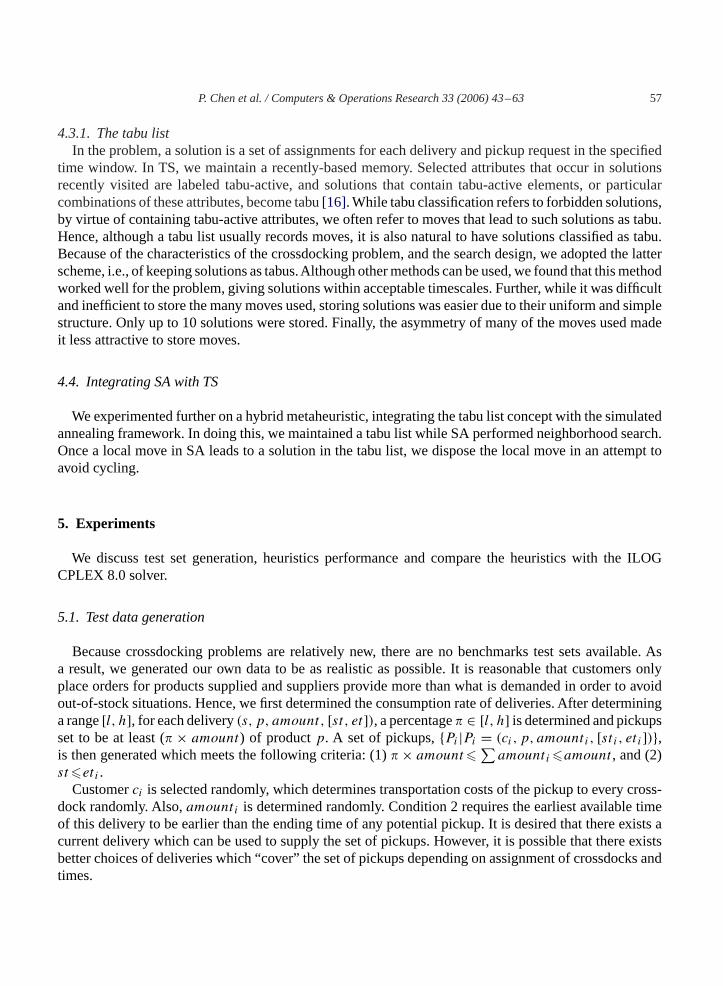
4.3.1. The tabu listIn the problem, a solution is a set of assignments for each delivery and pickup request in the specified

time window. In TS, we maintain a recently-based memory. Selected attributes that occur in solutionsrecently visited are labeled tabu-active, and solutions that contain tabu-active elements, or particularcombinations of these attributes, become tabu[16]. While tabu classification refers to forbidden solutions,by virtue of containing tabu-active attributes, we often refer to moves that lead to such solutions as tabu.Hence, although a tabu list usually records moves, it is also natural to have solutions classified as tabu.Because of the characteristics of the crossdocking problem, and the search design, we adopted the latterscheme, i.e., of keeping solutions as tabus.Although other methods can be used, we found that this methodworked well for the problem, giving solutions within acceptable timescales. Further, while it was difficultand inefficient to store the many moves used, storing solutions was easier due to their uniform and simplestructure. Only up to 10 solutions were stored. Finally, the asymmetry of many of the moves used madeit less attractive to store moves.

4.4. Integrating SA with TS

We experimented further on a hybrid metaheuristic, integrating the tabu list concept with the simulatedannealing framework. In doing this, we maintained a tabu list while SA performed neighborhood search.Once a local move in SA leads to a solution in the tabu list, we dispose the local move in an attempt toavoid cycling.

5. Experiments

We discuss test set generation, heuristics performance and compare the heuristics with the ILOGCPLEX 8.0 solver.

5.1. Test data generation

Because crossdocking problems are relatively new, there are no benchmarks test sets available. Asa result, we generated our own data to be as realistic as possible. It is reasonable that customers onlyplace orders for products supplied and suppliers provide more than what is demanded in order to avoidout-of-stock situations. Hence, we first determined the consumption rate of deliveries. After determininga range[l, h], for each delivery(s, p, amount, [st, et]), a percentage� ∈ [l, h] is determined and pickupsset to be at least (� × amount) of productp. A set of pickups,{Pi |Pi = (ci, p, amounti, [st i, et i])},is then generated which meets the following criteria: (1)� × amount� ∑

amounti�amount , and (2)st�et i .

Customerci is selected randomly, which determines transportation costs of the pickup to every cross-dock randomly. Also,amounti is determined randomly. Condition 2 requires the earliest available timeof this delivery to be earlier than the ending time of any potential pickup. It is desired that there exists acurrent delivery which can be used to supply the set of pickups. However, it is possible that there existsbetter choices of deliveries which “cover” the set of pickups depending on assignment of crossdocks andtimes.


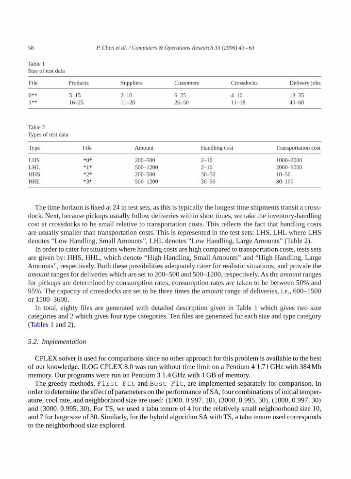
Table 1Size of test data

File Products Suppliers Customers Crossdocks Delivery jobs

0** 5–15 2–10 6–25 4–10 13–351** 16–25 11–20 26–50 11–18 40–60

Table 2Types of test data

Type File Amount Handling cost Transportation cost

LHS *0* 200–500 2–10 1000–2000LHL *1* 500–1200 2–10 2000–5000HHS *2* 200–500 30–50 10–50HHL *3* 500–1200 30–50 30–100

The time horizon is fixed at 24 in test sets, as this is typically the longest time shipments transit a cross-dock. Next, because pickups usually follow deliveries within short times, we take the inventory-handlingcost at crossdocks to be small relative to transportation costs. This reflects the fact that handling costsare usually smaller than transportation costs. This is represented in the test sets: LHS, LHL where LHSdenotes “Low Handling, Small Amounts”, LHL denotes “Low Handling, Large Amounts” (Table 2).

In order to cater for situations where handling costs are high compared to transportation costs, tests setsare given by: HHS, HHL, which denote “High Handling, Small Amounts” and “High Handling, LargeAmounts”, respectively. Both these possibilities adequately cater for realistic situations, and provide theamountranges for deliveries which are set to 200–500 and 500–1200, respectively. As theamountrangesfor pickups are determined by consumption rates, consumption rates are taken to be between 50% and95%. The capacity of crossdocks are set to be three times theamountrange of deliveries, i.e., 600–1500or 1500–3600.

In total, eighty files are generated with detailed description given in Table 1 which gives two sizecategories and 2 which gives four type categories. Ten files are generated for each size and type category(Tables 1 and 2).

5.2. Implementation

CPLEX solver is used for comparisons since no other approach for this problem is available to the bestof our knowledge. ILOG CPLEX 8.0 was run without time limit on a Pentium 4 1.71 GHz with 384 Mbmemory. Our programs were run on Pentium 3 1.4 GHz with 1 GB of memory.

The greedy methods,First Fit andBest Fit , are implemented separately for comparison. Inorder to determine the effect of parameters on the performance of SA, four combinations of initial temper-ature, cool rate, and neighborhood size are used:(1000,0.997,10), (3000,0.995,30), (1000,0.997,30)and(3000,0.995,30). For TS, we used a tabu tenure of 4 for the relatively small neighborhood size 10,and 7 for large size of 30. Similarly, for the hybrid algorithm SA with TS, a tabu tenure used correspondsto the neighborhood size explored.


Table 3Comparisons between greedy methods

Type No. of bests No. of bests average

First fit Best fit First fit Best fit

LHS 2 18 0 20LHL 6 14 5 15HHS 5 15 3 17HHL 5 15 4 16

5.3. Results and analysis

We compared the performance between CPLEX and the heuristics developed.

5.3.1. Comparisons between greedy methods for initial solutionsWe first analyzed the performance of the greedy methods. As shown inTable 3, the tightBest Fit

method performed better than the looseFirst Fit method most times where both best and averagesolution quality are considered. Here, each method was run on 20 files in each of the categories. InTable3, after one run of the 20 test sets for each category we report theno. of bestsfor each method, and after20 runs of the 20 test sets for each category and average the results, we measure theno. of bests averagewhich is the number of bests averages.

Best Fit method works extremely well with high handling cost files. This is because they requiremore careful assignments compared with low handling cost test cases, where fewer feasible initial solu-tions are found. The loose version of assigning tasks embedded inFirst Fit fails most of the timeas large free space at crossdocks is usually unavailable. Furthermore, theBest Fit requires much lessiterations in reaching a feasible solution if both start with an infeasible solution.Best Fit can find afeasible solution within the first 10 iterations, whereasFirst Fit usually takes tens or even hundredsof iterations to arrive into a feasible region. An extreme case is 038, whereFirst Fit failed to findany feasible solution within thousands of iterations in 21 out of 100 runs. The failure rate ofFirst Fitincreases when more deliveries and pickups are introduced, which make assignments more difficult. It isnoteworthy that file 038 is the only file for whichFirst Fit fails, suggesting that the problem solutionis intricate and may not depend on the numbers of deliveries, pickups, crossdocks and products alone,but on deliveries and pickups specifications.

5.3.2. Comparison between CPLEX and heuristicsSince CPLEX uses an exact method, we let it run without constraining time. However, CPLEX failed

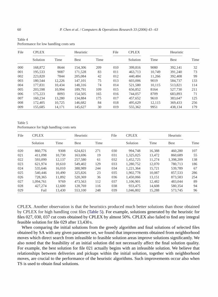
to find exact solutions before running out of memory in a number of cases.Table 4gives the best resultsobtained by CPLEX and by the heuristic algorithms on low handling costs test sets. There, we find a bestsolution for the heuristic is obtained by running all three heuristics over each of the 20 files 10 times.Experimental results using high handling cost sets are given inTable 5. From the table, we can see thatthe heuristics outperform CPLEX significantly not only in solution quality but also in computationaltimes (given in seconds). The heuristic provides better solution in all the test sets and can provide feasiblesolutions 7–50% better than those obtained by CPLEX, within only less than 10% the time spent of


Table 4Performance for low handling costs sets

File CPLEX Heuristic File CPLEX Heuristic

Solution Time Best Time Solution Time Best Time

000 168,872 8644 154,306 209 010 399,816 9080 392,141 32001 195,533 9087 171,528 83 011 463,713 10,749 391,240 73002 223,820 7844 205,084 42 012 440,484 11,266 392,408 99003 180,544 12,226 147,101 75 013 603,006 9019 584,737 133004 177,831 10,434 148,316 74 014 521,580 10,115 513,821 114005 203,598 10,994 189,791 109 015 656,852 8164 527,730 211006 175,223 8093 154,505 165 016 744,057 8709 683,893 71007 160,234 13,280 134,884 175 017 457,652 9610 383,647 125008 172,405 10,725 146,682 84 018 495,629 12,115 369,433 256009 155,685 14,171 145,627 30 019 555,362 9951 438,134 179

Table 5Performance for high handling costs sets

File CPLEX Heuristic File CPLEX Heuristic

Solution Time Best Time Solution Time Best Time

020 860,776 9308 624,821 271 030 994,748 16,388 460,280 107021 411,098 10,730 163,696 19 031 1,325,025 13,472 860,689 55022 593,099 12,137 257,580 61 032 1,452,725 11,274 1,398,209 138023 621,974 10,610 549,402 129 033 1,280,752 12,070 780,713 186024 535,646 16,010 388,989 244 034 1,221,364 15,721 539,789 67025 540,446 10,490 325,826 23 035 1,902,778 10,087 857,533 286026 728,365 11,892 520,369 36 036 1,450,066 13,151 873,583 254027 1,094,761 9769 473,563 112 037 1,106,901 12,482 483,044 89028 427,274 12,600 128,769 116 038 933,475 14,608 580,354 94029 Fail 13,430 553,100 248 039 1,046,802 15,288 573,745 96

CPLEX. Another observation is that the heuristics produced much better solutions than those obtainedby CPLEX for high handling cost files (Table 5). For example, solutions generated by the heuristic forfiles 027, 030, 037 cut costs obtained by CPLEX by almost 50%. CPLEX also failed to find any integralfeasible solution for file 029 after 13,430 s.

When comparing the initial solutions from the greedy algorithm and final solutions of selected filesobtained by SA with any given parameter set, we found that improvements obtained from neighborhoodmoves which direct search from infeasible to feasible solution areas improve solutions significantly. Wealso noted that the feasibility of an initial solution did not necessarily affect the final solution quality.For example, the best solution for file 021 actually begins with an infeasible solution. We believe thatrelationships between deliveries and pickups within the initial solution, together with neighborhoodmoves, are crucial to the performance of the heuristic algorithms. Such improvements occur also whenTS is used to obtain final solutions.


Table 6Comparisons (bests) using different parameter settings for SA+TS

Type No. of bests

(1000,0.997,10,4) (3000,0.995,10,4) (1000,0.997,30,7) (3000,0.995,30,7)LHS 4 4 7 5LHL 7 3 6 4HHS 4 3 6 7HHL 1 3 9 7

The bold values represent the highest score in each category. Where there is a tied score, both numbers are emboldened.

Table 7Comparisons (averages) using different parameter settings for SA+TS

Type No. of bests average

(1000,0.997,10,4) (3000,0.995,10,4) (1000,0.997,30,7) (3000,0.995,30,7)LHS 4 4 7 5LHL 3 4 8 5HHS 4 2 6 8HHL 1 0 7 12


5.3.3. Comparisons with parameter settingsWhen using different parameter sets, we found that SA worked best with a low initial temperature, a

slow cooling schedule and a large neighborhood size. For TS, better results were obtained when largeneighborhood sizes were used.

For the hybrid algorithm, the set of parameters,(1000,0.997,30,7) is best with small margin whenonly best solutions are considered (Table 6). Using averages, the parameters,(3000,0.995,30,7) givebetter results (Table 7) for high handling cost files. We found that, in general, low initial temperature andlarge neighborhood size was preferable.

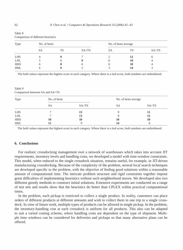
5.3.4. Comparison among heuristicsAs the heuristics perform better than CPLEX, we compare these heuristics.As can be seen fromTable 8,

TS outperforms SA and SA+TS on both best and average solutions obtained. This is expected since, in theproblem, neighborhood structure is not symmetric, which makes SA less competitive to TS. It is also notsurprising to see that the hybrid SA with TS does not improve the performance of SA alone much fromTable 9since both are SA-based. We can conclude that TS diversifies the solution space well, allowingacceptance of non-tabued solutions in a way which contributes to its good performance.


Table 8Comparison of different heuristics


SA TS SA+TS SA TS SA+TS

LHS 4 9 7 2 12 6LHL 5 6 9 6 10 4HHS 6 8 6 6 10 4HHL 6 9 5 3 14 3


Table 9Comparison between SA and SA+TS


SA SA+TS SA SA+TS

LHS 7 13 9 11LHL 7 13 8 12HHS 10 10 10 10HHL 11 9 14 6


6. Conclusions

For realistic crossdocking management over a network of warehouses which takes into account JITrequirements, inventory levels and handling costs, we developed a model with time-window constraints.This model, when reduced to the single crossdock situation, remains useful, for example, in JIT-drivenmanufacturing crossdocking. Because of the complexity of the problem, several local search techniquesare developed specific to the problem, with the objective of finding good solutions within a reasonableamount of computational time. The intricate problem structure and rigid constraints together imposegreat difficulties of implementing heuristics without such neighborhood moves. We developed also twodifferent greedy methods to construct initial solutions. Extensive experiments are conducted on a rangeof test sets and results show that the heuristics do better than CPLEX within practical computationaltimes.

In the problem, each pickup is restricted to collect a single product. In reality, customers can placeorders of different products at different amounts and wish to collect them in one trip to a single cross-dock. In view of future work, multiple types of products can be allowed in single pickup. In the problem,the inventory-handling cost at each crossdock is uniform for all products. This also can be adaptedto suit a varied costing scheme, where handling costs are dependent on the type of shipment. Multi-ple time windows can be considered for deliveries and pickups so that many alternative plans can beoffered.


References

[1] Napolitano M. Making the move to crossdocking—a practical guide. Warehousing Education and Research Council, 2002.[2] Bartholdi III JJ, Gue KR, Kang K. Throughput models for unit-load crossdocking,http://web.nps.navy.mil/∼krgue/

Publications/tput.pdf.[3] Shaffer B. Implementing the crossdocking operation. IIE Solutions 2000;30(5):20–3.[4] Bartholdi III JJ, Gue KR. The best shape for a crossdock. INFORMS national conference, San Antonio, TX, 2000.[5] Bartholdi JJ, Gue KR, Kang K. Staging freight in a crossdock. In: Proceedings of the International Conference on industrial

engineering and production management, Quebec City. Canada, 2001.[6] Gue KR, Kang K. Staging queues in material handling and transportation systems. Proceedings of the 2001 winter

simulation conference, 2001.[7] Bartholdi III JJ, Gue KR. Reducing labor costs in an LTL crossdocking terminal. Operations Research 2002;48(6):

823–32.[8] Donaldson H, Johnson EL, Ratliff HD, Zhang M, Schedule-driven cross-docking networks,http://www.isye.gatech.

edu/research/files/misc9904.pdf.[9] Ratliff HD, Vate JV, Zhang M. Network design for load-driven cross-docking systems,http://www.isye.gatech.

edu/research/files/misc9914.pdf.[10] Simchi-Levi D, Kaminsky P, Simchi-Levi E. Designing and managing the supply chain. 2nd ed., NewYork: McGraw-Hill;

2003.[11] Logistics today. 10 Best supply chains, December 2003,www.logisticstoday.com.[12] Logistics today. Execution at the dock, April 2004,www.logisticstoday.com.[13] Garey MR, Johnson DS. Computers and intractability—a guide to the theory of NP-completeness. NewYork:W.H. Freeman

and Company; 1979.[14] Cormen TH, Leiserson CE, Rivest RL, Stein C. Introduction to algorithms. 2nd ed., Cambridge, MA: MIT Press; 2001.[15] Kirkpatrick S, Gelatt CD, Vecchi MP. Optimization by simulated annealing. Science 1983;220(4598):671–80.[16] Glover F, Laguna M. Tabu search. Dordrecht: Kluwer Academic Publishers; 1997.

http://web.nps.navy.mil/krgue/Publications/tput.pdf

http://web.nps.navy.mil/krgue/Publications/tput.pdf

http://www.isye.gatech.edu/research/files/misc9904.pdf

http://www.isye.gatech.edu/research/files/misc9904.pdf

http://www.isye.gatech.edu/research/files/misc9914.pdf.

http://www.isye.gatech.edu/research/files/misc9914.pdf.

http://www.logisticstoday.com

http://www.logisticstoday.com

Documents

Multiple crossdocks with inventory and time windowsguoys/publications/CORCrossDock_Guo.pdf · Crossdocking studies have mostly been concerned with the physical layout of a crossdock