Embed Size (px)
Citation preview

Finland 2010 1
Multiple Criteria Optimization:Some Introductory Topics
Ralph E. SteuerDepartment of Banking & Finance
University of GeorgiaAthens, Georgia 30602-6253 USA

Finland 2010 3
Tchebycheff contour
probing direction
feasible region in criterion space
1 1max{ (x) }
max{ (x) }x
k k
f = z
f = zs .t . S∈
M
Z

Finland 2010 4
Production planningmin { cost }min { fuel consumption }min { production in a given geographical area }
River basin management
achieve { BOD standards }min { nitrate standards }min { pollution removal costs } achieve { municipal water demands }min { groundwater pumping }
Oil refiningmin { cost }min { imported crude }min { environmental pollution } min { deviations from demand slate }

Finland 2010 5
Sausage blending
min { cost }max { protein }min { fat } min { deviations from moisture target }
Portfolio selection in finance
min { variance }max { expected return }max { dividends }max { liquidity }max { social responsibility }
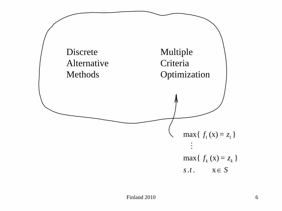
Finland 2010 6
Discrete Alternative Methods
Multiple Criteria Optimization
1 1max{ (x) }
max{ (x) }x
k k
f = z
f = zs .t . S∈
M
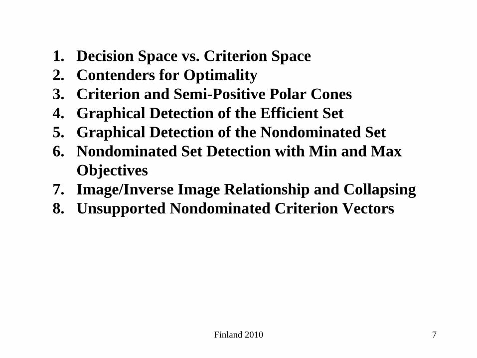
Finland 2010 7
1. Decision Space vs. Criterion Space2. Contenders for Optimality3. Criterion and Semi-Positive Polar Cones4. Graphical Detection of the Efficient Set5. Graphical Detection of the Nondominated Set6. Nondominated Set Detection with Min and Max
Objectives7. Image/Inverse Image Relationship and Collapsing8. Unsupported Nondominated Criterion Vectors

Finland 2010 8
1 1max{ (x) }
max{ (x) }x
k k
f = z
f = zs .t . S∈
M
11max{ c x }
max{ c x }x
kk
= z
= zs .t . S∈
M
But if all objectives and constraints are linear, we write
in which case we have a multiple objective linear program (MOLP).
In the general case, we write

Finland 2010 9
1 2 1
1 2 2
max{ }max{ 2 }. . x
x x zx x z
s t S
− =− + =
∈
z1
z2
Z
z1
z2z3
z4 = (3, -2)
= (0, 3)= (-1, 3)
1. Decision Space vs. Criterion Space
S
x1
x2
c1
c2
x1
x2
x3
x4 = (4, 1)
= (3, 3)
= (1, 2)
criterion objective outcome attribute evaluation image

Finland 2010 10
S
x1
x2
Morphing of S into Z as we change coordinate system

Finland 2010 11
Finland 2010 12

Finland 2010 13

Finland 2010 14
z1
z2
Z

Finland 2010 15
2. Contenders for Optimality
Points (criterion vectors) in criterion space are either nondominated or dominated.
Their points in decision space are either efficient or inefficient.
We are interested in nondominated criterion vectors and their efficient points because only they are contenders for optimality.
Finland 2010 16
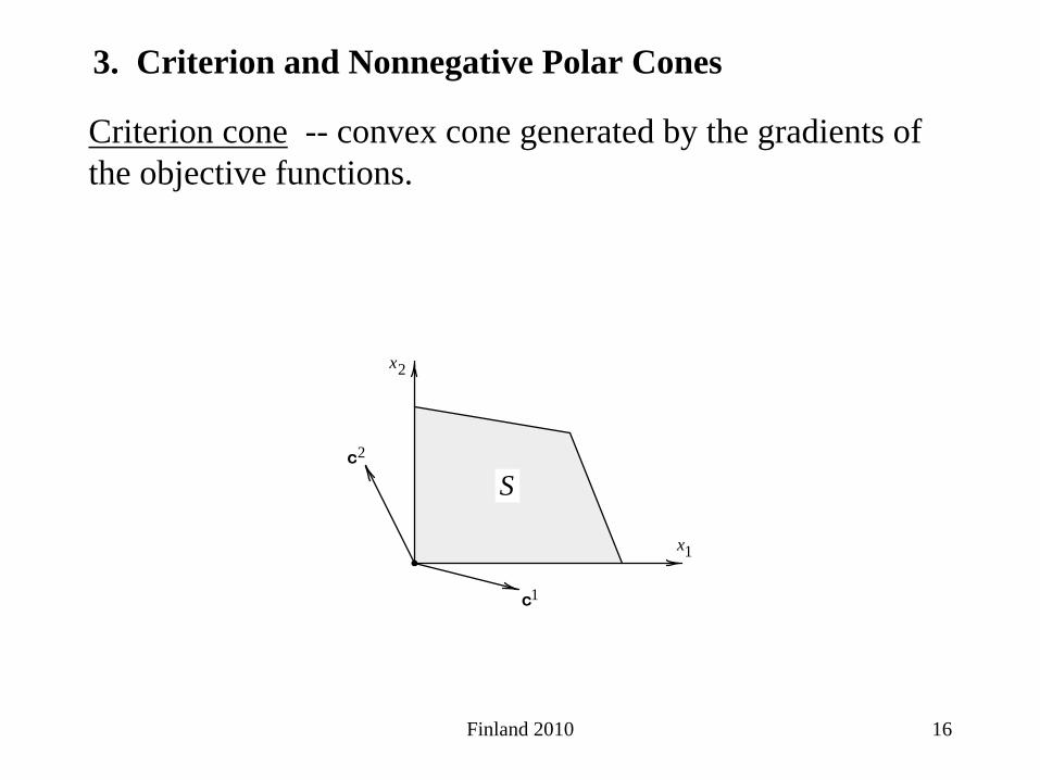
3. Criterion and Nonnegative Polar Cones
Criterion cone -- convex cone generated by the gradients of the objective functions.
S
x1
x2
c1
c2

Finland 2010 17
S
x1
x2
c1
c2
The larger the criterion cone (i.e., the more conflict there is in the problem), the bigger the efficient set.

Finland 2010 18
S
x1
x2
c1
c2
Nonnegative polar of the criterion cone -- set of vectors that make 90o or less angle with all objective function gradients. In the case of an MOLP, given by
{y : c y 0, 1, , }n iR i = k∈ ≥ K
Contains all points that dominate its vertex.

Finland 2010 19
4. Graphical Detection of the Efficient Set
Example 1
observe the criterion cone.
Sx1
x2
c1
c2

Finland 2010 20
form nonnegative polar cone
Sx1
x2
c1
c2

Finland 2010 21
Sx1
x2
c1
c2
x1
x2
x3
move it around

Finland 2010 22
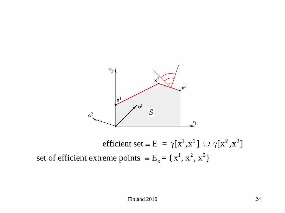
Sx1
x2
c1
c2
x1
x2
x3
1 2 2 3
1 2 3x
efficient set E = [x x ] [x x ]set of efficient extreme points E = {x , x , x }
, ,≡ γ ∪ γ
≡

Finland 2010 23
Sx1
x2
c1
c2
x1
x2
x3
1 2 2 3
1 2 3x
efficient set E = [x x ] [x x ]set of efficient extreme points E = {x , x , x }
, ,≡ γ ∪ γ
≡
Finland 2010 24
Sx1
x2
c1
c2
x1
x2
x3
1 2 2 3
1 2 3x
efficient set E = [x x ] [x x ]set of efficient extreme points E = {x , x , x }
, ,≡ γ ∪ γ
≡

Finland 2010 25
Sx1
x2
c1
c2
x1
x2
x3
Only when there is no intersection at other than the vertex of the cone

Finland 2010 26
S
x1
x2
c1
c2
Graphical Detection of the Efficient Set
Example 2
observe criterion cone

Finland 2010 27
S
x1
x2
c1
c2
form nonnegative polar cone

Finland 2010 28
1 2 3 4 5E = [x x ) {x } (x x ], ,∂ ∪ ∪ ∂
S
x1
x2
c1
c2
x1
x2
x3
x4
x5

Finland 2010 29
1 2 3 4 5E = [x x ) {x } (x x ], ,∂ ∪ ∪ ∂
S
x1
x2
c1
c2
x1
x2
x3
x4
x5
(observe that x2 and x4 are not efficient)

Finland 2010 30
Graphical Detection of the Efficient Set
Example 3
x1
x2
x1
x2
x3
x4
x5
x6
c1
c2
Note small size of criterion cone and that S consists of only 6 points.

Finland 2010 31
x1
x2
x1
x2
x3
x4
x5
x6
c1
c2
Small criterion cone results in a large nonnegative polar cone.
(this makes it harder for points to be efficient).

Finland 2010 32
6E = {x }Moving nonnegative polar cone around.
x1
x2
x1
x2
x3
x4
x5
x6
c1
c2

Finland 2010 33
z1
z2
Z
5. Graphical Detection of the Nondominated Set
To determine if a criterion vector in Z is nondominated, translate nonnegative orthant in Rk to the point.
move nonnegative orthant around
max max

Finland 2010 34
try to identify the entire nondominated set
z1
z2
Z

Finland 2010 35
z1
z2
Z
z1
z2
z3
1 2 2 3nondominated set N = [z z ] [z z ], ,γ≡ ∂ ∪

Finland 2010 36
z1
z2
Z
Now, move nonnegative orthant around.
max max

Finland 2010 37
z1
z2
Z
z1
z2 z3
z4
z5
z6

Finland 2010 38
z1
z2
Z
z1
z2 z3
z4
z5
z6

Finland 2010 39
z1
z2
Z
z1
z2 z3
z4
z5
z6

Finland 2010 40
z1
z2
Z
z1
z2 z3
z4
z5
z6
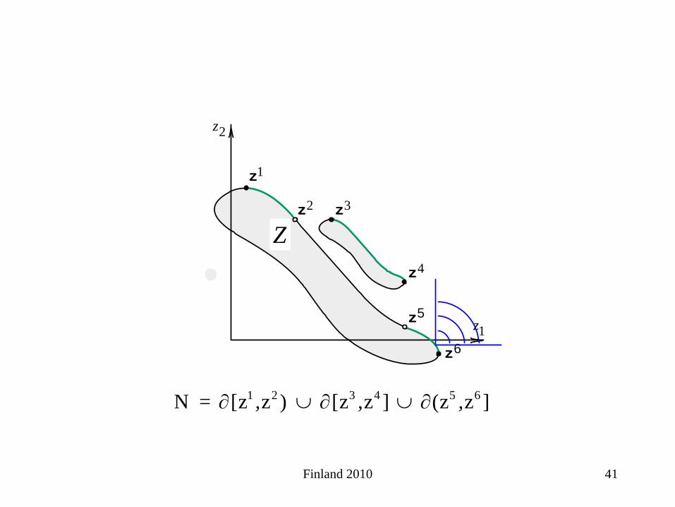
Finland 2010 41
z1
z2
Z
z1
z2 z3
z4
z5
z6
1 2 3 4 5 6N = [z z ) [z z ] (z z ], , ,∂ ∪ ∂ ∪ ∂
Finland 2010 42
z1
z2
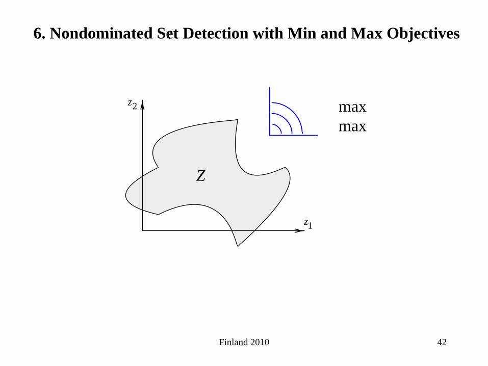
6. Nondominated Set Detection with Min and Max Objectives
max max
Z

Finland 2010 43
z1
z2
Z
max max

Finland 2010 44
z1
z2
Z
max max

Finland 2010 45
z1
z2
Z
max max

Finland 2010 46
z1
z2
Z
max max

Finland 2010 47
z1
z2 min max
Z

Finland 2010 48
z1
z2
Z
min max

Finland 2010 49
z1
z2
Z
min max

Finland 2010 50
z1
z2
Z
min max
Finland 2010 51
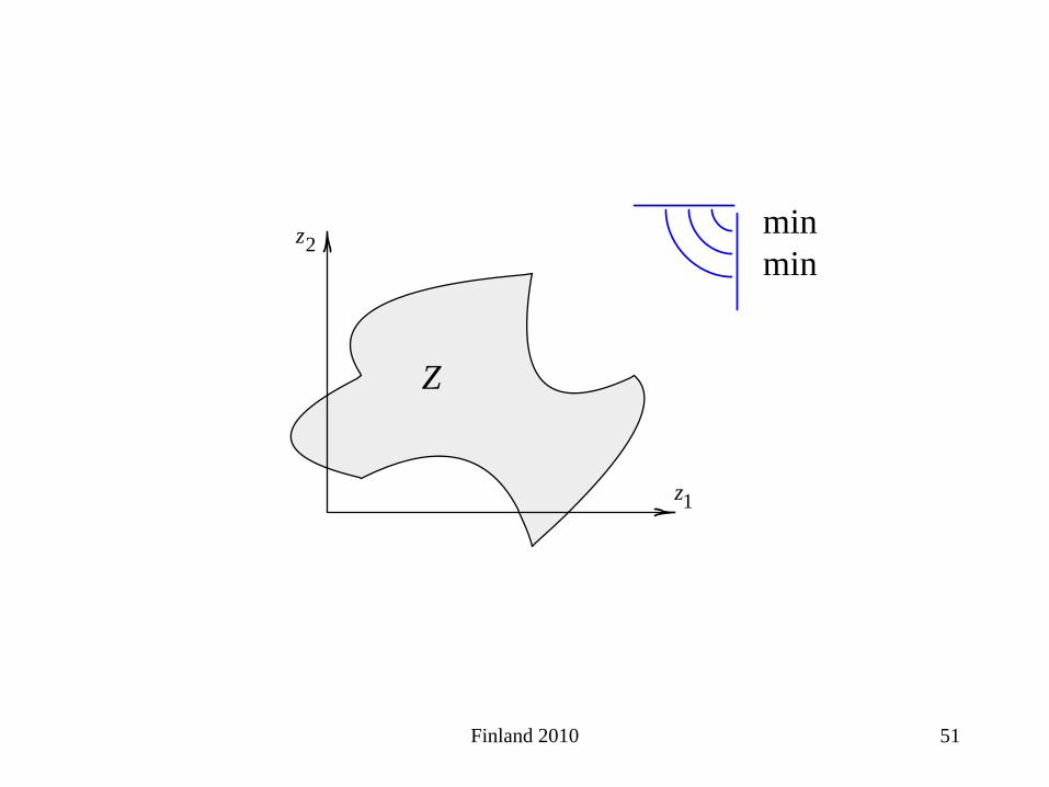
z1
z2min min
Z
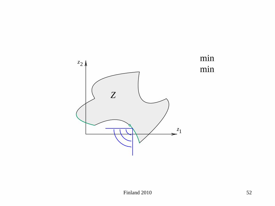
Finland 2010 52
z1
z2
Z
min min

Finland 2010 53
z1
z2 max min
Z

Finland 2010 54
z1
z2
Z
max min

Finland 2010 55
Let z . Then z is if and only if there doesnot exist another z Z such that for all and for
at least one Otherwise z is .
Let x . Then x is if and
i i j j
Z nondominatedz z i z z
j . , dominated
S efficient
∈∈ ≥ >
∈ only its criterion vector zis nondominated. Otherwise x is ., inefficient
In other words,
image of an efficient point is a nondominated criterion vector inverse image of a nondominated criterion vector is an eff point

Finland 2010 56
1 2 3 1
1 2 3 2
max{3 2 }max{ }. . x unit cube
x x x zx x x z
s t S
+ − =− + + =∈ =
7. Image/Inverse Image Relationship and Collapsing
dimensionality of S is n, but dimensionality of Z is k.
x1x5
x2 x6
x4 x8
x3 x7
x1
x2
x3
c1
c2
= (1, 1, 0)
S
z4
z1
z2
z1
z3
z6
z2
z5
z7
z8
2
Z = (2, 1)
= (4, 0)
= (-2, 1)
Finland 2010 57
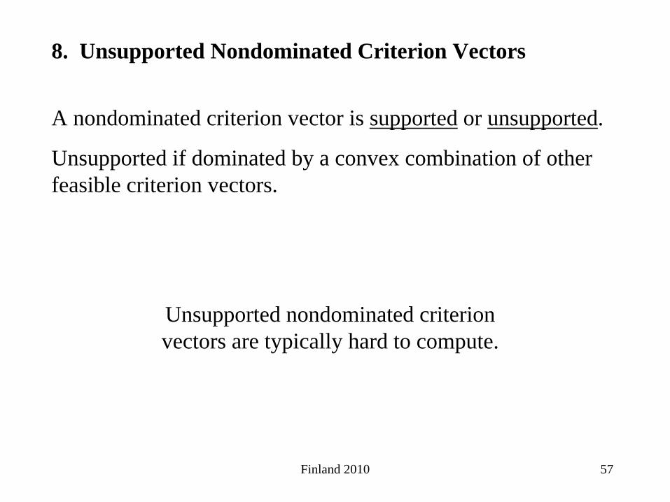
8. Unsupported Nondominated Criterion Vectors
A nondominated criterion vector is supported or unsupported.
Unsupported if dominated by a convex combination of other feasible criterion vectors.
Unsupported nondominated criterion vectors are typically hard to compute.

Finland 2010 58
1 2 1
1 2 2
max{ 9 }max{ 3 8 }. . x
x x zx x z
s t S
− + =− =∈
z1
z2x2
x115
c2
c1
2

Finland 2010 59
1 2 1
1 2 2
max{ 9 }max{ 3 8 }. . x
x x zx x z
s t S
− + =− =∈
z1
z2x2
x115
c2
c1
2
-15
x1 x2 x3
z3
z2
z1
x4
x5
z4
z5

Finland 2010 60
1 2 1
1 2 2
max{ 9 }max{ 3 8 }. . x
x x zx x z
s t S
− + =− =∈
supp 1 2 3 4 5
unsupp supp
N = N {z , z , z , z , z }
N N
Z
Z=
= −
z1
z2x2
x115
c2
c1
2
-15
x1 x2 x3
z3
z2
z1
x4
x5
z4
z5

Finland 2010 61
z1
z2
Z z1
z2
supp 1
unsupp 2
N {z }N {z }
=
=

Finland 2010 62
Multiple Criteria Optimization:An Introduction (Continued)
Ralph E. SteuerDepartment of Banking & Finance
University of GeorgiaAthens, Georgia 30602-6253 USA

Finland 2010 63
Recall9. Ideal way?10. Contours, Upper Level Sets and Quasiconcavity11. More-Is-Always-Better-Than-Less vs. Quasiconcavity12. ADBASE13. Size of the Nondominated Set14. Criterion Value Ranges over Nondominated Set15. Nadir Criterion Values16. Payoff Tables17. Filtering18. Stamp/Coin Example19. Weighted-Sums Method20. e-Constraint Method

Finland 2010 64
1 2 1
1 2 2
max{ }max{ 2 }. . x
x x zx x z
s t S
− =− + =
∈
z1
z2
Z
z1
z2z3
z4 = (3, -2)
= (0, 3)= (-1, 3)
S
x1
x2
c1
c2
x1
x2
x3
x4 = (4, 1)
= (3, 3)
= (1, 2)
Recall

Finland 2010 65
Z
zo
z1
z2
1max{ ( , , )}. . (x) 1, ,
x
k
i i
U z zs t f z i k
S= =∈
K
K
Assess a decision maker’s utility function UUUUUUaand solve: kU R R→
9. Ideal Way?
Finland 2010 66
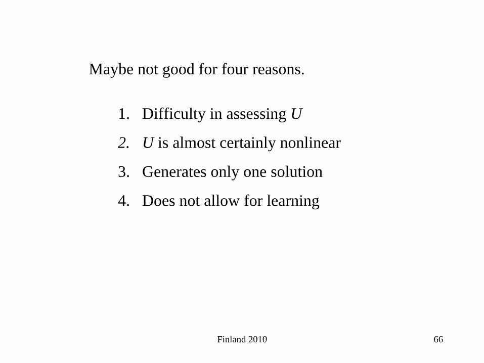
Maybe not good for four reasons.
1. Difficulty in assessing U
2. U is almost certainly nonlinear
3. Generates only one solution
4. Does not allow for learning

Finland 2010 67
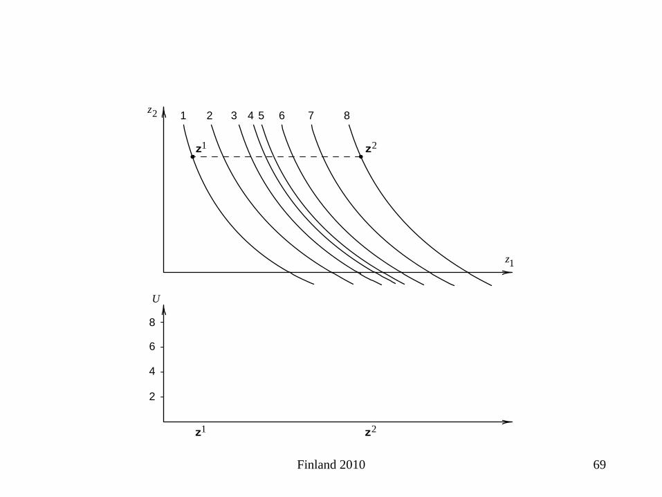
A U is quasiconcave if all upper level sets are convex.
10. Contours, Upper Level Sets, and Quasiconcavity
1 2 3 4 5 6 7 8
U
z1
z2
z1
6
4
2
8

Finland 2010 68
1 2 3 4 5 6 7 8
U
z1
z2
z1 z2
z2z1
6
4
2
8
Finland 2010 69
1 2 3 4 5 6 7 8
U
z1
z2
z1 z2
z2z1
6
4
2
8

Finland 2010 70
1 2 3 4 5 6 7 8
U
z1
z2
z1 z2
z2z1
6
4
2
8

Finland 2010 71
1 2 3 4 5 6 7 8
U
z1
z2
z1 z2
z2z1
6
4
2
8
Quasiconcave functions have at most one top.
Finland 2010 72
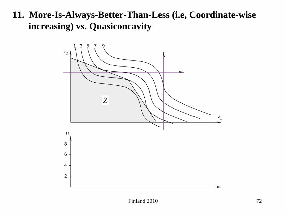
11. More-Is-Always-Better-Than-Less (i.e, Coordinate-wise increasing) vs. Quasiconcavity
1 3 5 7 9
U
z1
z2
6
4
2
8
Z

Finland 2010 73
More-is-always-better-than-less does not imply that all local optima are global optima
1 3 5 7 9
z1
z2
Zz1
z2
z1 is a local optimum, but z2 is the global optimum.

Finland 2010 74
1 3 5 7 9
U
z1
z2
6
4
2
8
Z
z3
z4
z4z3
More-is-always-better-than-less does not imply quasiconcavity

Finland 2010 75
1 3 5 7 9
U
z1
z2
6
4
2
8
Z
z3
z4
z4z3
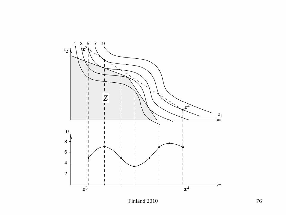
Finland 2010 76
1 3 5 7 9
U
z1
z2
6
4
2
8
Z
z3
z4
z4z3
Finland 2010 77
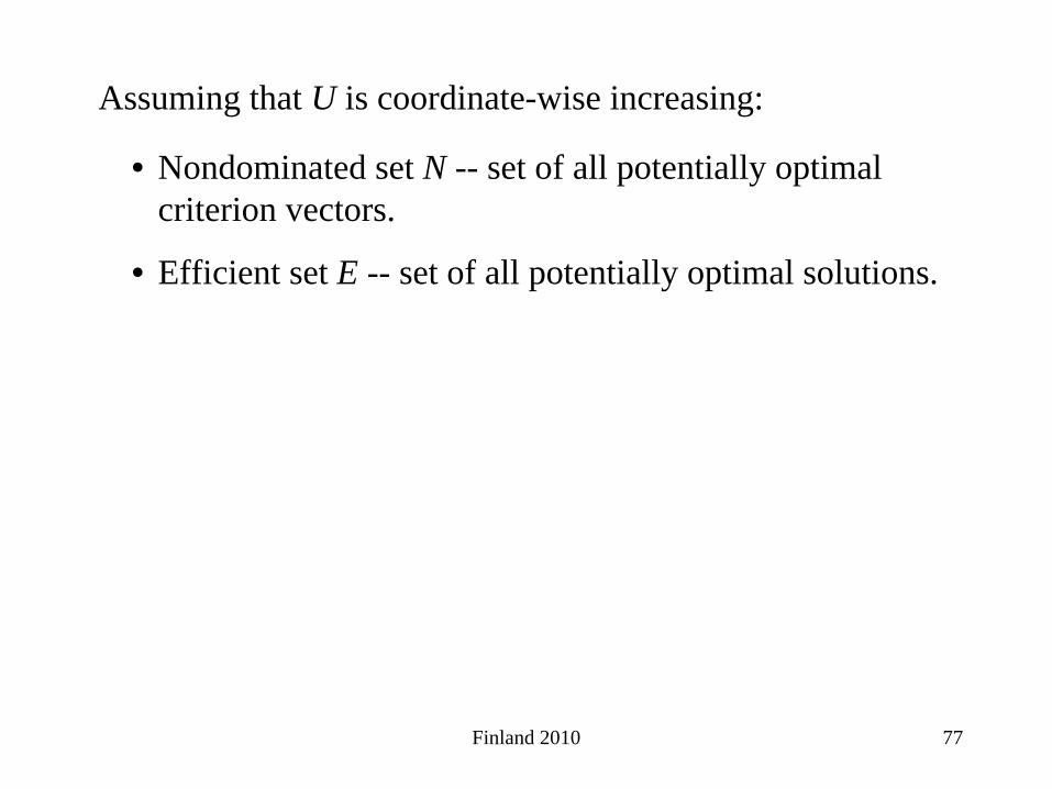
• Nondominated set N -- set of all potentially optimal criterion vectors.
• Efficient set E -- set of all potentially optimal solutions.
Assuming that U is coordinate-wise increasing:

Finland 2010 78
12. ADBASE
In an MOLP, of course, efficient set is a portion of the surface of S, and nondominated set is a portion of the surface of Z.
ADBASE is for MOLPs. It computes all of the extreme points of S that efficient, and hence all of the vertices of Z that are nondominated in an MOLP.

Finland 2010 79
13. Size of the Efficient and Nondominated Sets
MOLP ave efficient aveproblem size extreme pts CPU time3 x 100 x 150 13,415 363 x 250 x 375 285,693 5,5734 x 50 x 75 19,921 245 x 35 x 45 15,484 145 x 60 x 90 414,418 1,223

Finland 2010 80
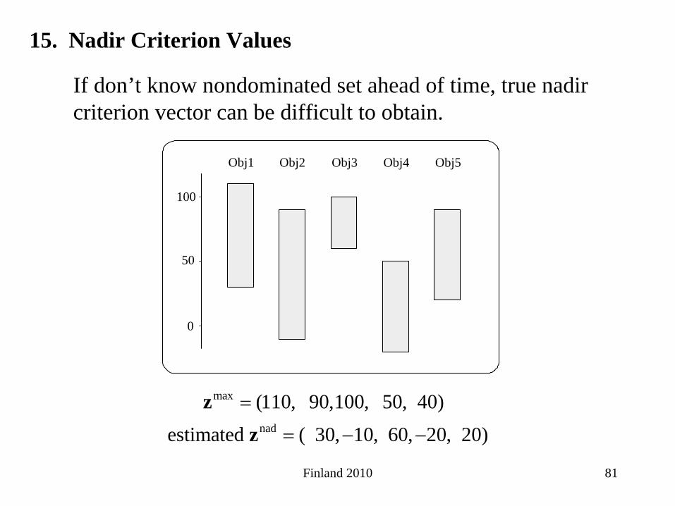
14. Criterion Value Ranges over the Nondominated Set
Obj1 Obj2 Obj3 Obj4 Obj5
100
0
50
The lower bounds on the ranges are called nadir criterion values.
If know nondominated set ahead of time, can “warm up” decision maker with following information.
Finland 2010 81
Obj1 Obj2 Obj3 Obj4 Obj5
100
0
50
max
nad
(110, 90,100, 50, 40)estimated ( 30, 10, 60, 20, 20)
=
= − −
zz
15. Nadir Criterion Values
If don’t know nondominated set ahead of time, true nadir criterion vector can be difficult to obtain.

Finland 2010 82
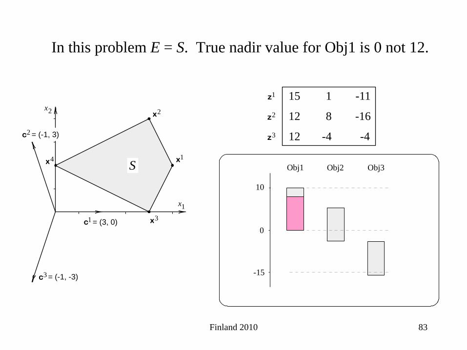
Obj1 Obj2 Obj3
15
-15
0
16. Payoff TableObtained by individually maximizing each objective over S. But minimum column values often over-estimate nadir values.
x1
x2
c2
c3
c1
S
= (3, 0)
= (-1, 3)
= (-1, -3)
x1
x2
x3
x4
15 1 -11
12 8 -16
12 -4 -4
z1
z2
z3
Finland 2010 83
Obj1 Obj2 Obj3
10
-15
0
In this problem E = S. True nadir value for Obj1 is 0 not 12.
x1
x2
c2
c3
c1
S
= (3, 0)
= (-1, 3)
= (-1, -3)
x1
x2
x3
x4
15 1 -11
12 8 -16
12 -4 -4
z1
z2
z3
Finland 2010 84
The larger the problem, the greater the likelihood that the payoff table column minimum values will be wrong.
After about 5 x 20 x 30, most will be wrong.

Finland 2010 85
17. Filtering
Reducing 8 vectors down to a dispersed subset of size 5
z1
z2
z3
z4
z5
z6
z7
z8
z1
z2

Finland 2010 86
First point z1
always retained by filter.
z1
z2
z3
z4
z5
z6
z7
z8
z1
z2

Finland 2010 87
z2
retained by filter, but z3 and z5 discarded.
z1
z2
z3
z4
z5
z6
z7
z8
z1
z2

Finland 2010 88
z4
retained by filter, but z8
discarded.
z1
z2
z3
z4
z5
z6
z7
z8
z1
z2

Finland 2010 89
z6
retained by filter, but z7
discarded.
z1
z2
z3
z4
z5
z6
z7
z8
z1
z2
Wanted 5 but got 4. Reduce neighborhood, then do again. After a number of iterations, will converge to desired size.

Finland 2010 90
Z
z1
z2 (Coins)
(Stamps)
z1
z2
z3
18. Stamp/Coin Example

Finland 2010 91
Z
z1
z2 (Coins)
(Stamps)
z1
z2
z3

Finland 2010 92
19. Weighted-Sums Method
1. decision-maker’s preferences.
2. scale in which the objectives are measured (e.g., cubic feet versus board feet of lumber).
3. shape of the feasible region
But how to pick the weights because they are a function of
max{ Cx}. . x
T
s t Sλ∈
11max{ c x }
max{ c x }. . x
kk
z
zs t S
=
=∈
M
May also get flip-flopping behavior.

Finland 2010 93
Purpose of weighted-sums approach is to obtain information from the DM to create a λ-vector that causes “composite gradient” λTC in the weighted-sums program
to point in the same direction as the utility function gradient.
max{ Cx}. . x
T
s t Sλ∈

Finland 2010 94
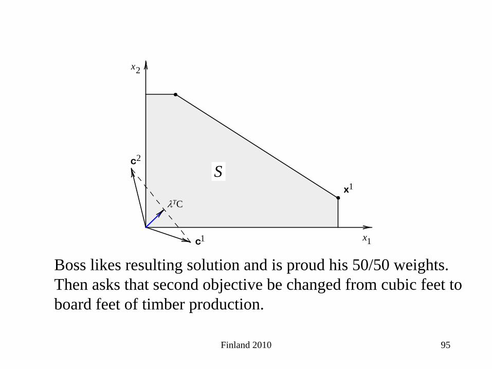
Boss says to go with 50/50 weights.
2.
x1
x2
S
c1
c2
Finland 2010 95
Boss likes resulting solution and is proud his 50/50 weights. Then asks that second objective be changed from cubic feet to board feet of timber production.
x1
x2
S
c1
c2
x1
λTC

Finland 2010 96
With 50/50 weights, this causes composite gradient to point in a different direction. Get a completely different solution.
x1
x2
S
c1
c2
x1
x2
λTC

Finland 2010 97
3.
Boss says use 60/40 weights.
Finland 2010 98
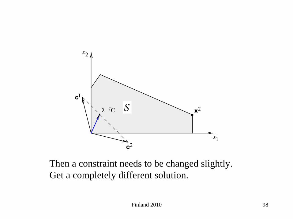
Then a constraint needs to be changed slightly. Get a completely different solution.
Finland 2010 99
z1
z2
Z
z1
z2
z3
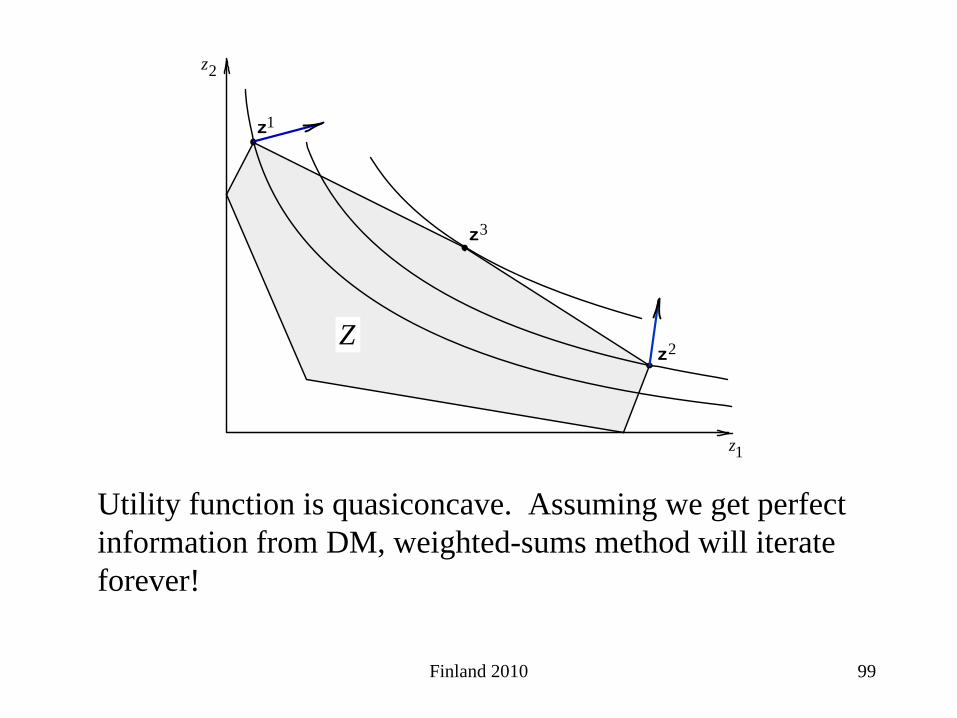
Utility function is quasiconcave. Assuming we get perfect information from DM, weighted-sums method will iterate forever!

Finland 2010 100
11max{ c x }
max{ c x }. . x
kk
z
zs t S
=
=∈
M
20. e-Constraint Method
max{ c x }
. . c xx
jj
ii
z
s t e i jS
=
≥ ≠∈
Basically trial-and-error

Finland 2010 101
max{ c x }
. . c x
c xx
pp
mm
ee
z
s t e
eS
=
≥
≥∈
x1
cmce
cp
x2eeem

Finland 2010 102
22. Overall Interactive Algorithmic Structure23. Vector-Maximum/Filtering24. Goal Programming25. Lp-Metrics26. Weighted Lp-Metrics27. Reference Criterion Vector28. Wierzbicki’s Aspiration Criterion Vector Method29. Lexicographic Tchebycheff Sampling Program30. Tchebycheff Procedure (overview)31. Tchebycheff Procedure (in more detail)32. Tchebycheff Vertex λ-Vector33. How to Compute Dispersed Probing Rays34. Projected Line Search Method35. List of Interactive Procedures

Finland 2010 103
set controlling parameters for the 1st iteration
solve optimizationproblem(s)
examine criterion vector results
done
reset controlling parametersfor the next iteration
stopy
start
Controlling Parameters:
weighting vector ei RHS values aspiration vector others
22. Overall Interactive Algorithmic Structure
Finland 2010 104
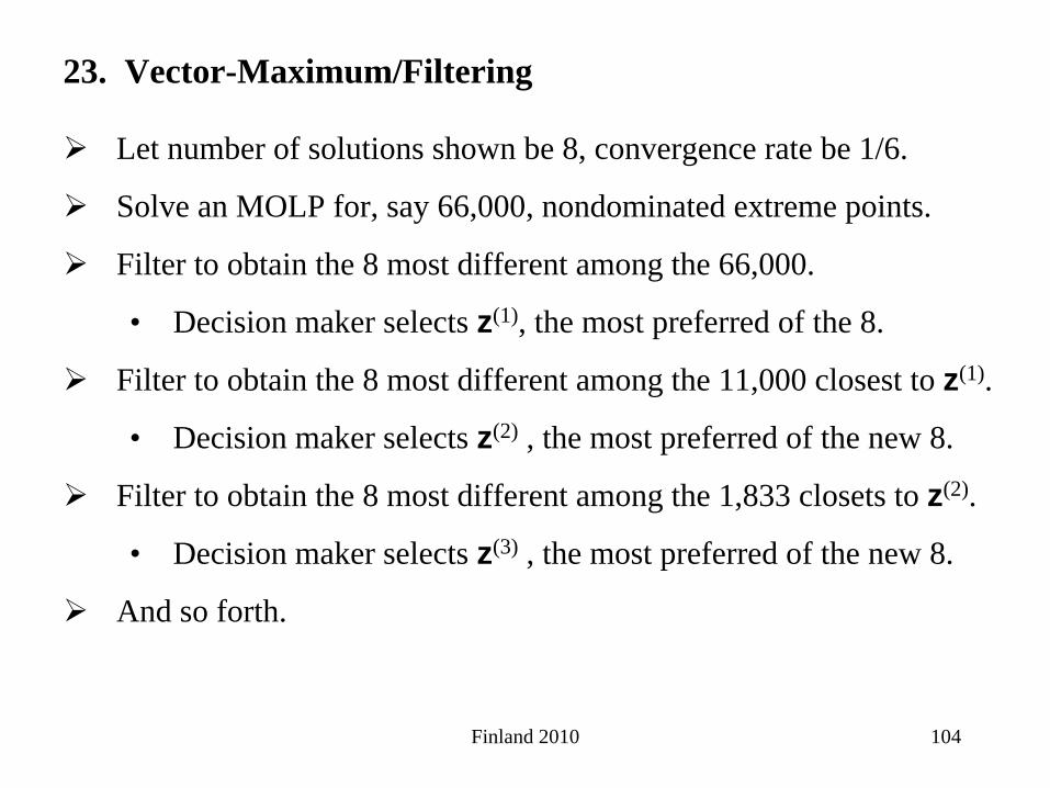
23. Vector-Maximum/Filtering
Let number of solutions shown be 8, convergence rate be 1/6.
Solve an MOLP for, say 66,000, nondominated extreme points.
Filter to obtain the 8 most different among the 66,000.
• Decision maker selects z(1), the most preferred of the 8.
Filter to obtain the 8 most different among the 11,000 closest to z(1).
• Decision maker selects z(2) , the most preferred of the new 8.
Filter to obtain the 8 most different among the 1,833 closets to z(2).
• Decision maker selects z(3) , the most preferred of the new 8.
And so forth.

Finland 2010 105
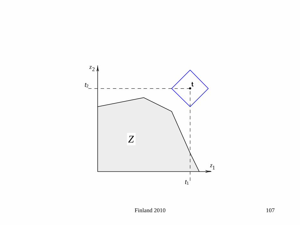
24. Goal Programming
11
22
33
max{ c x }
achieve{ c x }
min{ c x }. . x
z
z
zs t S
=
=
=∈
1 1 2 2 2 2 3 31
1 12
2 2 23
3 3
min{ }
. . c x
c x
c xx
all , 0i i
w d w d w d w d
s t d t
d d t
d tS
d d
− − − − + + + +
−
− +
+
− +
+ + +
+ ≥
+ − =
+ ≤∈
≥
Must choose a target vector and then select deviational variable weights.
Goal programming uses weighted L1 -metric.
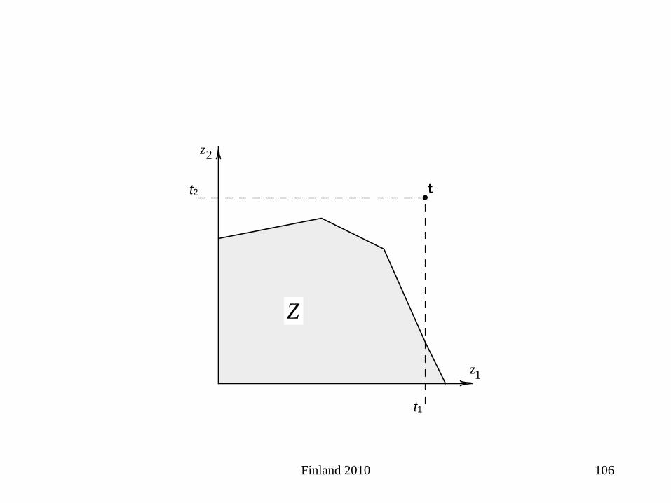
Finland 2010 106
z1
z2
Z
tt2
t1
Finland 2010 107
z1
z2
Z
tt2
t1

Finland 2010 108
z1
z2
Z
tt2
t1
z1

Finland 2010 109
z1
z2
Z
tt2
t1

Finland 2010 110
z1
z2
Z
tt2
t1
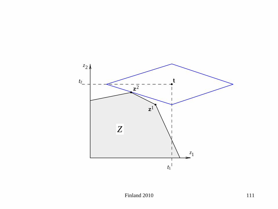
Finland 2010 111
z1
z2
Z
tt2
t1
z1
z2

Finland 2010 112
25. Lp-Metrics
**z
{ }
1
**1**
**
1
1, 2,
max
ppki ii
p
i ii k
z z pz z
z z p
=
≤ ≤
⎧ ⎡ ⎤− =⎪⎪ ⎢ ⎥⎣ ⎦− = ⎨⎪ − = ∞⎪⎩
∑ K

Finland 2010 113
{ }
1
**1**
**
1
1, 2,
max
ppki ii
p
i ii k
z z pz z
z z p
=
≤ ≤
⎧ ⎡ ⎤− =⎪⎪ ⎢ ⎥⎣ ⎦− = ⎨⎪ − = ∞⎪⎩
∑ K
**z

Finland 2010 114
{ }
1
**1**
**
1
1, 2,
max
ppki ii
p
i ii k
z z pz z
z z p
=
≤ ≤
⎧ ⎡ ⎤− =⎪⎪ ⎢ ⎥⎣ ⎦− = ⎨⎪ − = ∞⎪⎩
∑ K
**z
Finland 2010 115
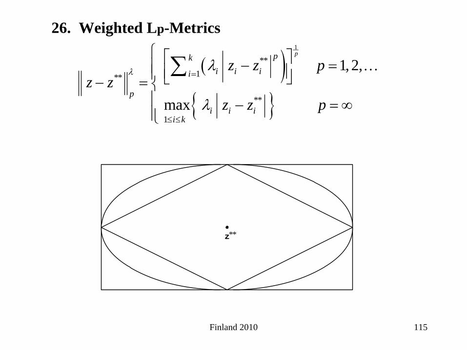
26. Weighted Lp-Metrics
( ){ }
1
**1**
**
1
1, 2,
max
ppki i ii
p
i i ii k
z z pz z
z z p
λ λ
λ
=
≤ ≤
⎧ ⎡ ⎤− =⎪ ⎢ ⎥⎪ ⎣ ⎦− = ⎨⎪ − = ∞⎪⎩
∑ K
**z

Finland 2010 116
( ){ }
1
**1**
**
1
1, 2,
max
ppki i ii
p
i i ii k
z z pz z
z z p
λ λ
λ
=
≤ ≤
⎧ ⎡ ⎤− =⎪ ⎢ ⎥⎪ ⎣ ⎦− = ⎨⎪ − = ∞⎪⎩
∑ K
**z

Finland 2010 117
( ){ }
1
**1**
**
1
1, 2,
max
ppki i ii
p
i i ii k
z z pz z
z z p
λ λ
λ
=
≤ ≤
⎧ ⎡ ⎤− =⎪ ⎢ ⎥⎪ ⎣ ⎦− = ⎨⎪ − = ∞⎪⎩
∑ K
**z

Finland 2010 118
( ){ }
1
**1**
**
1
1, 2,
max
ppki i ii
p
i i ii k
z z pz z
z z p
λ λ
λ
=
≤ ≤
⎧ ⎡ ⎤− =⎪ ⎢ ⎥⎪ ⎣ ⎦− = ⎨⎪ − = ∞⎪⎩
∑ K
**z

Finland 2010 119
z1
z2
Z
3
27. Reference Criterion Vector
Constructed so as to dominate every point in the nondominated set
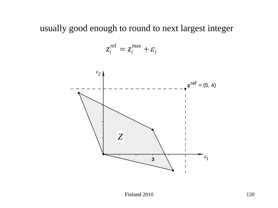
Finland 2010 120
z1
z2
zref
Z
3
= (5, 4)
usually good enough to round to next largest integer
ref maxi i iz z ε= +

Finland 2010 121
Z
z1
z2
28. Wierzbicki’s Reference Point Procedure

Finland 2010 122
Z
z1
z2 zref

Finland 2010 123
Z
z1
z2 zref
q(1)
First iteration

Finland 2010 124
Z
z1
z2 zref
q(1)

Finland 2010 125
Z
z1
z2 zref
q(1)

Finland 2010 126
Z
z1
z2 zref
q(1)

Finland 2010 127
Z
z1
z2 zref
q(1)
z(1)

Finland 2010 128
Z
z1
z2 zref
q(2)
Second iteration

Finland 2010 129
Z
z1
z2 zref
q(2)

Finland 2010 130
Z
z1
z2 zref
q(2)
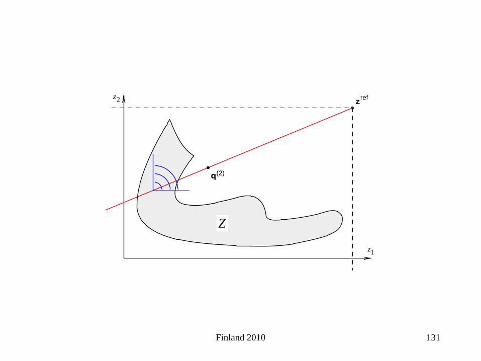
Finland 2010 131
Z
z1
z2 zref
q(2)

Finland 2010 132
Z
z1
z2 zref
q(2)
z(2)

Finland 2010 133
Third iteration
Z
z1
z2 zref
q(3)

Finland 2010 134
Z
z1
z2 zref
q(3)

Finland 2010 135
Z
z1
z2 zref
q(3)

Finland 2010 136
Z
z1
z2 zref
q(3)
z(3)
Finland 2010 137
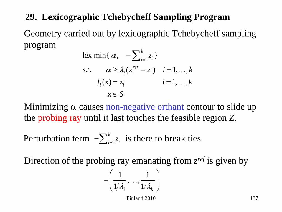
1lex min{ , }
. . ( ) 1, ,(x) 1, ,
x
kii
refi i i
i i
z
s t z z i kf z i k
S
α
α λ=
−
≥ − == =∈
∑K
K
Geometry carried out by lexicographic Tchebycheff sampling program
Minimizing α
causes non-negative orthant contour to slide up the probing ray until it last touches the feasible region Z.
1 1, ,1 1i kλ λ⎛ ⎞
−⎜ ⎟⎝ ⎠
K
Direction of the probing ray emanating from zref is given by
Perturbation term 1
kii
z=
−∑ is there to break ties.
29. Lexicographic Tchebycheff Sampling Program
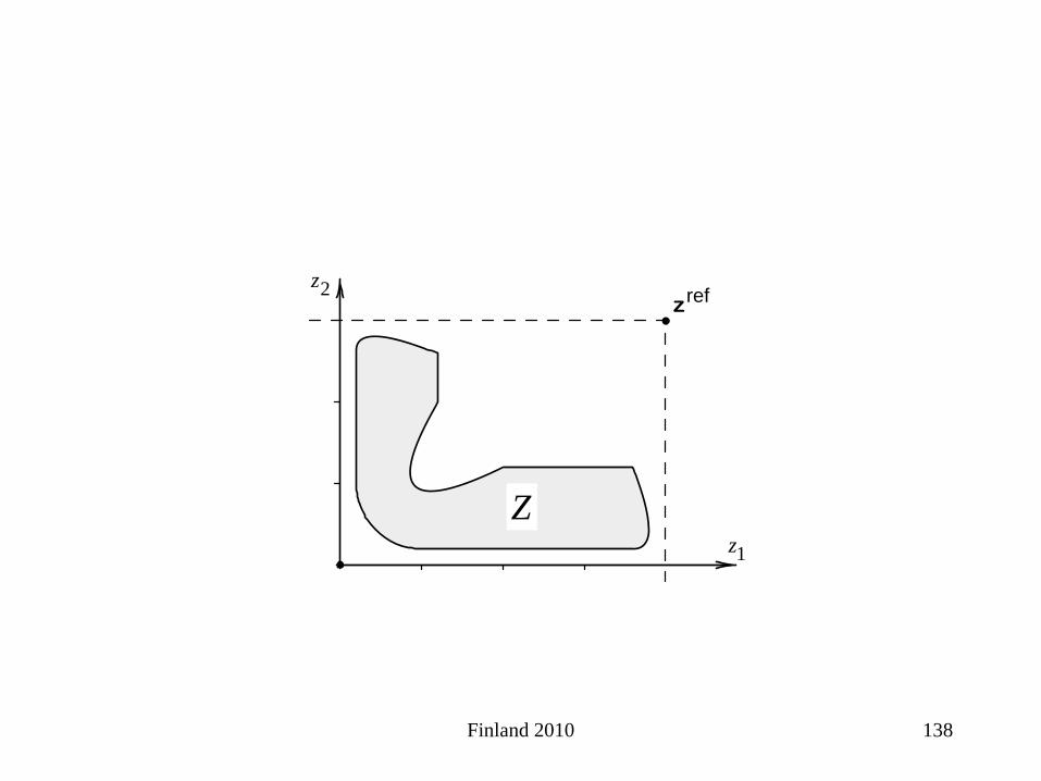
Finland 2010 138
z1
z2zref
Z

Finland 2010 139
z1
z2zref
Z
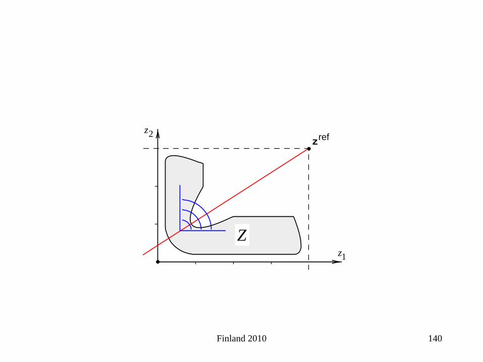
Finland 2010 140
z1
z2zref
Z

Finland 2010 141
z1
z2zref
Z
z1
z2
Two lexicographic minimum solutions, but both nondominated

Finland 2010 142
30. Tchebycheff Method (Overview)
zref
z1
z2
Z

Finland 2010 143
First iteration
zref
z1
z2

Finland 2010 144
zref
z1
z2
z(1)
Finland 2010 145
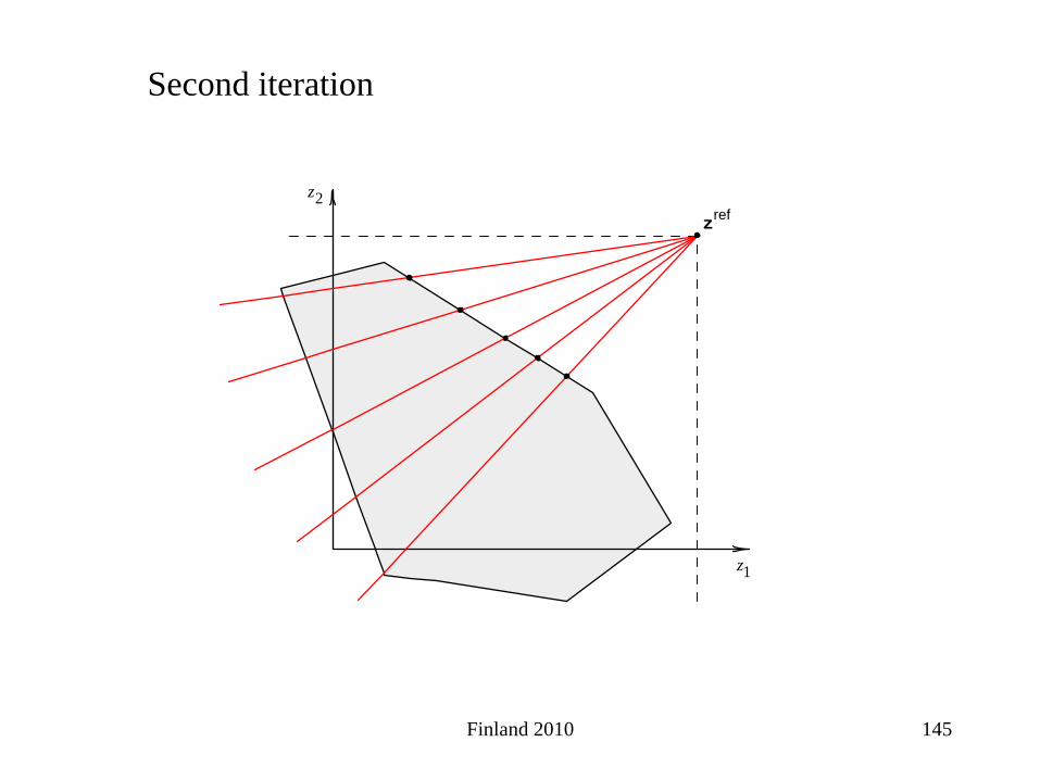
Second iteration
zref
z1
z2

Finland 2010 146
zref
z1
z2
z(2)

Finland 2010 147
Third iteration
zref
z1
z2
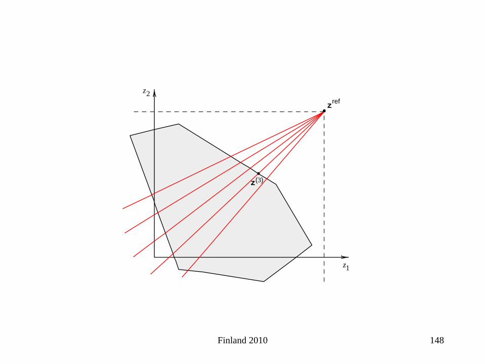
Finland 2010 148
zref
z1
z2
z(3)

Finland 2010 149
set controlling parameters for the 1st iteration
solve optimizationproblem(s)
examine criterion vector results
done
reset controlling parametersfor the next iteration
stopy
start
Controlling Parameters:
target vector, weights q(i) aspiration vectors λi multipliers

Finland 2010 150
31. Tchebycheff Method (in more detail)
Let P = number of solutions to be presented to the DM at each iteration = 4
Let r = reduction factor = 0.5
Let t = number of iterations = 4

Finland 2010 151
Now, form reference criterion vector zref.
z1
z2
Z

Finland 2010 152
z1
z2
Z
zref
Now, form Λ(1) and obtain 4 dispersed λ-vectors from it.
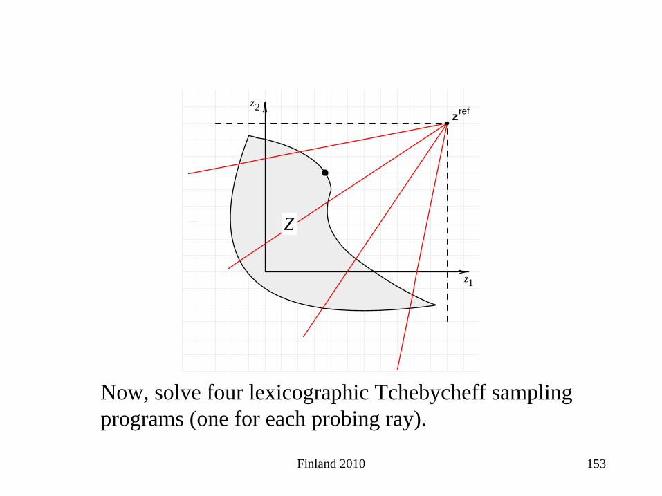
Finland 2010 153
Now, solve four lexicographic Tchebycheff sampling programs (one for each probing ray).
z1
z2
Z
zref

Finland 2010 154
Now, select most preferred, designating it z(1).
z1
z2
Z
zref

Finland 2010 155
Now, form Λ(2) and obtain 4 dispersed λ-vectors from it.
z1
z2
Z
zref
z(1)

Finland 2010 156
32. Tchebycheff Vertex λ-Vector
zref
z(1)

Finland 2010 157
33. How to Compute Dispersed Probing Rays
zref
z(1)

Finland 2010 158
1
(1)(1) (1)
1
1 1k
i ref refji i j jz z z z
λ−
=
⎡ ⎤= ⎢ ⎥
− −⎢ ⎥⎣ ⎦∑

Finland 2010 159
Now, solve four lexicographic Tchebycheff sampling programs.
z1
z2
Z
zref

Finland 2010 160
Now, select most preferred, designating it z(2).
z1
z2
Z
zref

Finland 2010 161
Now, form Λ(3) and obtain 4 dispersed λ-vectors from it.
z1
z2
Z
zref
z(2)

Finland 2010 162
Now, solve four lexicographic Tchebycheff sampling programs.
z1
z2
Z
zref
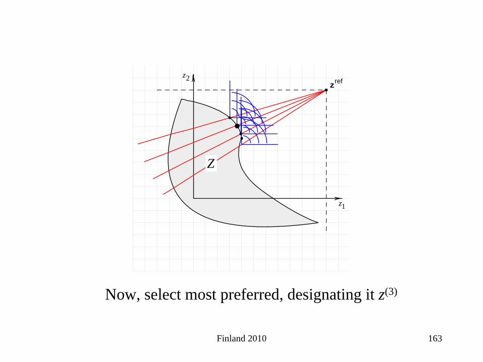
Finland 2010 163
Now, select most preferred, designating it z(3)
z1
z2
Z
zref

Finland 2010 164
Now, form Λ(4) and obtain 4 dispersed λ-vectors from it.
z1
z2
Z
zref
z(3)

Finland 2010 165
And so forth.
z1
z2
Z
zref

Finland 2010 166
34. Projected Line Search Method
z1
z2
z(1)
Like driving across surface of moon.

Finland 2010 167
z1
z2
z(1)
q(2)

Finland 2010 168
z1
z2
z(1)
q(2)

Finland 2010 169
z1
z2
z(1)
z(2)
q(2)
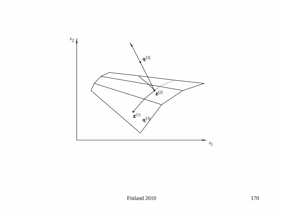
Finland 2010 170
z1
z2
z(1)
z(2)
q(3)
q(3)

Finland 2010 171
z1
z2
z(1)
z(2)
q(3)
z(3)

Finland 2010 172
z1
z2
z(1)
z(2)
z(3)
Drive straight awhile, turn, drive straight awhile, turn, drive straight awhile, and so forth.

Finland 2010 173
1. Weighted-sums (traditional)
2. e-constraint method (traditional)
3. Goal programming (mostly US, 1960s)
4. STEM (France & Russia, 1971)
5. Geoffrion, Dyer, Feinberg procedure (US, 1972)
6. Vector-maximum/filtering (US, 1976)
7. Zionts-Wallenius Procedure (US & Finland, 1976)
8. Wierzbicki’s reference point method (Poland, 1980)
9. Tchebycheff method (US & Canada, 1983)
10. Satisficing tradeoff method (Japan, 1984)
11. Pareto Race (Finland, 1986)
12. AIM (US & South Africa, 1995)
13. NIMBUS (Finland, 1998)
35. List of Interactive Procedures

Finland 2010 174
The End
![PhD Thesis Seminar Presentation 2 - Jyväskylän yliopistousers.jyu.fi/~timoh/kurssit/jatkoksem/FC.pdf · [Agilent E6474A Drive Test Network Optimization Platform] 9 . UNIVERSITY](https://img.pdfslide.us/doc/110x75/5ac794707f8b9acb688bc49c/phd-thesis-seminar-presentation-2-jyvskyln-timohkurssitjatkoksemfcpdfagilent.jpg)