ENGINEERING MONOGRAPHS

United States Department of the Interior

BUREAU OF RECLAMATION

No. 2 (7~~4--~}

e. I

MULTIPLE CORRELATION IN

FORECASTING SEASONAL RUNOFF

By Perry M. Ford

Denver,. Colorado

June 1959 50 cents

United States Department of the Interior

FRED A. SEATON, Secretary

Bureau of Reclamation

FLOYD E. DOMINY, Commissioner GRANT BLOODGOOD, Assistant Commissioner and Chief Engineer

Engineering Monograph

No. 2 (second revision)

MULTIPLE CORRELATION IN

FORECASTING SEASONAL RUNOFF

by Perry M. Ford Engineer. Hydrology Branch

Division of Project Investigations

Technical Information Branch Denver Federal Center

Denver, Colorado

ENGINEERING MONOGRAPHS are published in limited editions for the technical staff of the Bureau of Reclamation and interested technical circles in government and private agencies. Their purpose is to record developments, inno­vations, and-progress in the engineering and scientific techniques and practices that are em­ployed in the planning, design, construction, and operation of Reclamation structures and equip­ment. Copies may be obtained from the Bureau of Reclamation, Denver Federal Center, Denver, Colorado, and Washington, D. C.

INTRODUCTION

NOTATION ••••.

THE FORECASTING PROBLEM Major Factors Affecting Run-off

CONTENTS

PRINCIPLE OF MULTIPLE LINEAR CORRELATION

APPLICATION OF MULTIPLE LINEAR CORRELATION

. . .

Multiple Correlation Coefficient. Standard Deviation. and Standard

. . ..

1

1

3 3

3

5

Error of Estimate • • • • • • • • • • • • • • • • • • • • 13 Standard Deviation of Regression Coefficients· • • • • • • 14 Limits of Error Related to Run-off Season Precipitation 17 Reliability of Individual Forecast • . • • • • • • • • • . • • 17 Computations for the April 1. 1950 Forecast. with 0. 90 Limits of Error. 19

CHARACTERISTICS OF .LIMITS OF ERROR FOR TWO TYPES OF FORECASTING EQUATION . • . • • • • • . ••••••••••.

PRACTICAL CONSIDERATIONS PERTAINING TO CORRELATION ANALYSES . Precision of Multiple Regression Coefficients . • • • • • • •• Significance of Difference between Correlation Coefficients •••• Nun1ber of Variables • • • • • • • • • • • • .- ••••••••••• Correlation between Independent Variables •••••••••••• Inclusion of Run-off Season Precipitation; Revision of Forecast

SHORTCUT METHOD FOR SCREENING POSSIBLE CONTRIBUTING FACTORS • • • • • • • • • • ••••

CHANGE OF DEPENDENT VARIABLE

ELIMINATION OF AN INDEPENDENT VARIABLE ••

COMPARISON OF ERRORS OF FORECAST.

CONSISTENCY OF RECORDS •••••••••

DISCHARGE FROM LARGE RIVER BASINS •

MULTIPLE CORRELATION COMPUTATIONS ON ELECTRONIC COMPUTIN"G MACHINES • • • • • • • • • • • • • • • • • • • • •

. .. .

Forms and Procedures. • Form A •• . . . . -. Form B. Form C •• Form D.

i

20

21 21 21 22 23 23

24

26

33

34

35

38

38

39 39 39 40 40

Number

1.

2a.

2b.

3.

4.

5.

Number

1.

2.

3.

4.

5.

6.

7.

8.

9.

10.

11.

12.

13.

LIST OF FIGURES

Correlation of observed vs. estimated April-July run-off, South Fork Boise River . . . . . . . . . . . . . . . . . . .

Relationship between observed flows and preliminary estimates, Colorado River . • . . . . . . . . . . . . . . . . . . . . . .

Relationship between departures in Figure 2a and antecedent precipitation . . . . . . . . . . . . . . . . . . . . . . . . . .

Correlation of observed vs. estimated Apri11 july run-off, Colorado River at Cameo, Colorado . . . . . . . . . .

Double mass diagram of precipitation data, individual stations vs. average for the area ........... .

Double mass diagram, estimated vs. observed run-off

LIST OF TABLES

Records of Precipitation, Snow-Water Equivalents, and Run-off, South Fork Boise River above Anderson Ranch Dam, Idaho .

Extensions of Data from Table 1 . . . . . . . . . . . . . . . . . . .

Product Sums Corrected to Departures from the Means, with Check

Evaluation of Multiple Regression Coefficients

£he_sk on Computation of Regression Coefficients and Solutions for R, S, and a ................ .

Areas under the Normal Probability Curve . . . . . . . . . . . . . .

Combined Solution for Evaluating the b Coefficients and c Matrix • .

Back Solution on c Values ............. .

Records of Precipitation, Snow-Water Equivalents, and Run-off, Colorado River at Cameo, Colorado ....

Doolittle Solution for Evaluation of c Matrix • .

Extensions with X1

Extensions Corrected to Departures from the Mean

Che_£k ~Computation of Regression Coefficients, and Solutions for R, S, and a . . . . . . . . . . . . . . . . . . . . . . . . . .

ii

11

25

25

27

36

37

6

7

8

9

10

12

15

16

28

29

31

31

32

INTRODUCTION

Mast hydrologic phenomena are products of multiple causation. Flood season dis­charge is associated with several variables, antecedent in time, among which are ac­cumulated precipitation# ground -water con­ditions~ and temperature. The effect of each of these causal or associated factors (independent variables) upon flood season run-off (dependent variable) may be deter­mined by multiple correlation~ and the re­sulting equation applied to estimating run­off volume in advance of the flood season. Studies initiated by the writer in 1938 have shown that the use of multiple correlation in forecasting seasonal run-off is a practi­cable and useful tool in the analysis of hy­drologic data.

This monograph was prepared for use by Bureau employees who must deal with problems of hydrological forecasting. It assumes at the very least a reasonably thorough grounding in the fundamentals of statistics. Anyone not sure of these fun­damentals~ or who is using multiple cor­relation for the first time, should either make his initial study with someone ex­perienced with the procedure~ or have his results checked by such a person.

Emphasis has been placed on the appli­cation of statistical methods rather than on the development of the mathematical theory upon which the methods depend. Attention is directed to fundamental prin­ciples which have an important effect on the reliability of the analysis~ such as length

· of record# limitation on the number of inde­pendent variables# selection of major causal factors, and significance of relationship.

In developing forecasting procedures a unique problem is confronted in that an im­portantcausalfactor# run-off season precip-

itatio~ is unknown at the date of forecasting. A means of forecasting rnn-off and of deter­mining the reliability of the forecast under these conditions is included. A procedure is offered to facilitate the screening of likely causal or associated factors other than the more obviously important variables. The examples selected illustrate how widely basins differ, and how a given basin re­quired analysis in accordance with the phys­ical and climatological characteristics pe­culiar to that basin.

TIE work involved in problems like those illustrated here consists of computations which can be carried out rapidly on a key­board-type calculating machine. About three man-days should be adequate for solution of such problems# exclusive of exploratory work and tabulation of basic data. Accuracy of the work is assured by the numerous checks on computations.

The labor involved may be materially reduced through the use of automatic com­puting machines# especially for problems involving long periods of record and 4 or 5 variables; or where forecasting procedures with possible alternatives are to be de­veloped for several streams ~e'!uiring fore­casts for several dates. Such solutions may conveniently include computation of the de­partures and extensions required in setting up the normal equations, the regression co­efficients and their standard errors# the multiple correlation coefficient, the stand­ard error of estimate# and the constant term. This revision of the monograph has been expanded to include an adaptation of multiple correlation computations to machine processing. The procedure is arranged for programming on various types of high-speed computers.

NOTATION

Y =Estimated value of the dependent variable (run-off)

X1 =Observed values of the dependent variable

X2# X3# ••• # Xn = Observed values of independent variables

x2# x3# ••• # xn = Deviations from mean values of x 2# x 3, ••• , Xn# respectively

1

y =Deviation from mean value of Y

a = Constant term of the regression equation

h2, h3, •.. ~ bn = Regression coefficients

hi = Any particular regression coefficient

CTb = Standard deviation of a regression coefficient, b

um = Standard error of the mean

CTy-x1

= Standard error of individual estimate

(Y - X 1)0 _ 90 = Error of individual forecast for 0. 90 probability

n = Number of events, or nth term in a series

m = Number· of constants in the regression equation

S = Standard error of estimate

R =Coefficient of multiple correlation

r =Coefficient of simple correlation

M 1 = Mean of the dependent variable

M2~ M3, •.• , Mn =Means of independent variables

My = Mean value of Y

Mx = Mean value of X

Z =Residual

A bar above a symbol (R, S, etc.) means that the degrees of freedom have been taken into account in the evaluation.

The notation follows that of Ezekiel's Methods of Correlation Analysis. For this reason (and because of its excellence), Ezekiel's text if suggested to anyone who wishes to review the fundamentals of cor­relation analysis. A complete reference is given on page ·3.

The symbol n is used in this text to indicate (1) some definite number of ob­servations, and (2) the nth term in a series. In each case~ the position of the letter clearly indicates its function, since in the first case it is never a subscript, while in the latter it is always a subscript.

Subscripts of the form b 12 . 34 are

2

occasionally used. The first of the two digits to the left of the dot (not a decimal point) represents the dependent variable~ while the second of the two represents the independent variable whose effect is stated. In subscripts having only one digit to the left of the dot, such as R1• 234, that digit represents the dependent vari­able. In all cases, the digits to the right of the dot represent the independent vari­able or variables held constant during the process.

Frequently the subscript notations may be abbreviated without danger of ambiguity; thus b12 . 34 may be identified by the use of the subscript 2 only, i.e.~ b2; such abbreviations are employed in numerous instances in this discussion.

/ THE FORECASTING PROBLEM

The method of multiple correlation is applied here to estimating run-off volume in advance of the flood season. This run­off comes principally from melting snow during the spring and early summer months. In the following example, a forecast is made on April 1 of the April-through-July flow at a given point on a particular stream.

The problem is to develop a multiple regression equation which summarizes the relationships of past hydrologic events

. ·as evidenced in records of natural run-off and of factors contributing to run-off, and to determine the reliability of this equation as a means of forecasting. Such an equa­tion is also referred to as an estimating equation, particularly when applied to a period of known run-off as a means of pro­viding a comparison between estimated and observed flows; or as a forecasting equation when predicting future run-off. Since the equation is based on natural flow, the fore­cast value will require correction for stor­age and diversions which affect the flood season run-off volume.

Major Factors Affecting Run-off

Although precipitation and run -off are logically related as cause and effect, the amounts of precipitation occurring in dif­ferent seasons contribute to run-off in different ways and in varying degrees. Recorded precipitation during the fall and early winter months provides an index of gr~und-water conditions. In some basins precipitation during the preceding summer

shows a relationship with current flood sea­son run-off. Snow surveysl or winter pre­cipitation records provide an index of the moisture accumulated in the snow cover that is available for release upon melting. Temperatures during the accumulation pe-riod show an appreciable effect on flood season run-off in some basins. An added factor to be considered in the analysis is precipitation during the run-off season. In regions where this factor is of major im­portance, its inclusion in the analysis con­tributes to greater precision in computing the regression coefficients which apply to the other independent variables, and to greater confidence in the forecast and use­fulness of the forecasting procedure.

It will be noted that seasonal precipi­tation is used rather than monthly values. This grouping of months is necessary in order to reduce the number of independent variables to a practicable minimum. The reduction in number of variables is partie­ularly important in view of the relatively short periods of record available for the development of forecasting procedures. Seasonal values are desirable, also, be­cause of the tendency toward normality of distribution exhibited by records for longer time intervals. These and other require­ments for insuring reliability of the fore­cast will become more evident as the basic principles of multiple correlation are re­viewed.

1 The method of measuring water equivalents of snow by means of sampling the snow cover at specified courses is ex­.plained in Snow Surveying. Miscellaneous Publication No. 380. U. S. Department of Agriculture. June 1940.

PRINCIPLE OF MULTIPLE LINEAR CORRELATION

This ·brief explanation of the mathe­matical principle of multiple correlation is included to show how the method may be applied in practical problems of hy­drology. Only the more elementary alge­braic statements are used. Derivations and proofs of the basic formulas given may be obtained from textbookS on statistics. 2

2 A general treatment of the principle of multiple correla­tion is contained in: Ezekiel. Mordecai. Methods of Corre­lation Analysis. 2nd Edition. John Wiley and Sons. New York. 1941.

3

Multiple correlation may be regarded as an extension of the simple, two-variable correlation procedure. A linear regression involving two variables may be expressed by an equation of the form

Y = · a + bX • • • • • • • • • • • • • ( 1)

in which Y is a dependent variable, being dependent upon values assigned to an in­dependent variable, X. When the above

equation is plotted on rectangular coor­dinates, the two constants, a and b, are the Y intercept and the slope, respec­tively, of the resulting regression line.

For two or more in(iependent variables the relationship may be represented by a multiple linear regression equation as

in which Y, as before, is dependent upon values assigned to the several independent variables, and a is a constant term. The independent variables are designated as x2, x3' ... ' xn, and the several regres­sian coefficients as b2, b 3, ••• , bn' the subscripts relating to their corresponding independent variables.

Upon determination of the values of these respective multiple regression co­efficients, b 1s, and of the constant, a, a value for Y may be computed from equa­tion (2) for any set of values of the inde­pendent variables. In developing an equa­tion of this type for forecasting run-off from a particular drainage area, values of a and b are determined from an anal­ysis of pertinent climatological and run-off records. The analysis is based on the premise that the correct values of the con­stants are those which yield estimates of Y, the dependent variable, which are in closest agreement with the observed values for a period of record.

With this minimum deviation between estimated and observed values as a cri­terion, the values of the constants may be determined mathematically. In accordance with the method of least squares, the agree­ment between computed estimates, Y, and observed values, xl' is closest when the sum of the squared deviations is a mini­mum, that is, when

has a minimum value.

It can be shown by the calculus that the condition of least squares is satisfied for a two-variable linear relationship by the ;following normal equations:

4

in which x2 and xl represent observed values of the independent and dependent variables, respectively, and n is the num­ber of observations.

The relationship between independent and dependent variables expressed by equa­tions ( 3) and ( 4) may be expressed also in terms of deviations from the means (small x 1s) by the equations

( 5)

a=M -M b xl x2

(6)

The values of a and b may be determined from these two equations. Then these values substituted in eq. (1) will permit an estimate, Y, of the dependent variable (run-off) for any magnitude of the inde­pendent variable (precipitation).

In the solution of problems in multiple correlation, equations in the form of ( 5) and (6) are employed in which the several variables are expressed in terms of devi­ations from means.

For a three-variable problem (two in­dependent and one dependent variables) the equations are ·

and for a four-variable problem they are

2 L(x2)b2 +L (x2x3)b3

+L;(x2x4)b4 = L(x1x2)

L (x2x 4)b2 + L;(x3x 4)b3

2 + L(x4)b4 = ~(x1x4)

• • ( 8)

Values of a and b determined by the solu­tion of these equations are substituted in eq. (2) to yield a forecasting equation.

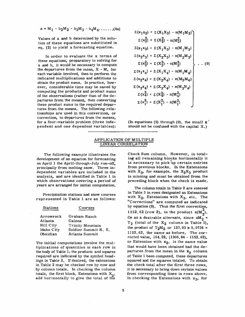
In order to evaluate the x terms of these equations, preparatory to solving for a and b, it would be necessary to compute the departures from the mean, X - M, for each variable involved, then to perform the indicated multiplications and additions to obtain the product sums. In practice, how­ever, considerable time may be saved by computing the products and product sums of the observations (rather than of the de­partures from the means), then converting these product sums to the required depar­tures from the means. The following rela­tionships are used in this conversion, or correction, to departures from the means, for a four-variable problem (three inde­pendent and one dependent variables):

E(x1x2) = t(X1X2)- n(M1M2)

t (x~) = t (X~) - n(M~) E(~ 1x3 ) = t (X 1X 3) - n{M 1M 3)

E {x2x3) t (X2X 3) - n{M2M 3)

t (x~) E {X~) - n(M~)

E(x1x4) = E (X1X4) - n(M 1M 4)

t (x2x 4) = t (X2X 4) - n(M3M4 )

E (x3x4) = E (X3X 4) - n(M 3N 4}

E (x~) = t (X~} - n(M~)

E (x~) = E (X~} - n(M~)

.. (9}

(In equations ( 5) through (9), the small X '

should not be confused with the capital X. )

APPLICATION OF MULTIPLE LINEAR CORRELATION.

The following example illustrates the development of an equation for forecasting on April 1 the April-through-July run-off, principally from melting snow. Three in­dependent variables are included in the analysis, and are identified in Table 1 in wh,ich observations covering a period of years are arranged for initial computation.

Precipitation stations and snow courses represented in Table 1 are as follows:

Stations

Arrowrock Atlanta Hill City Idaho City Obsidian

Courses

Graham Ranch Galena Trinity Mountain Soldier Summit R. S. Atlanta Summit

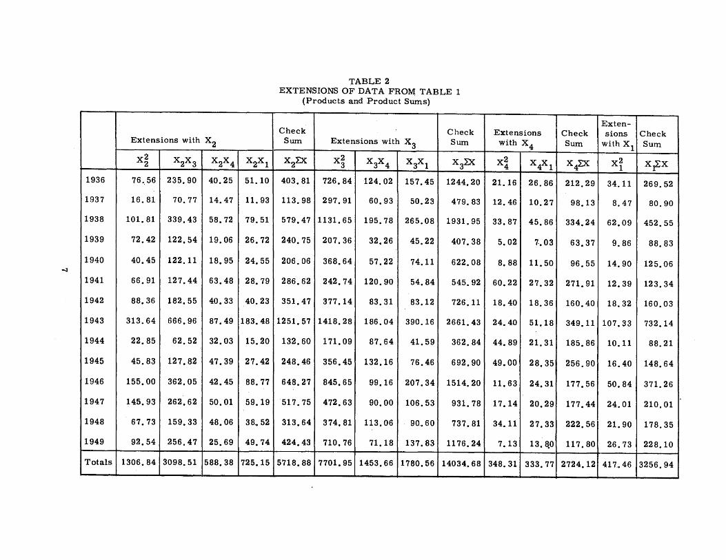
The initial computations involve the mul­tiplications of quantities in each row in the body of Table 1; the products and squares required are indicated by the symbol head­ings in Tabie 2. If desired, the extensions in Table 2 may be checked row by row and by column totals. In checking the column totals, the first block, Extensions with X

2,

add horizontally to give the total of tne

5

Check Sum column. However,. in total­ing all remaining blocks horizontally it is necessary to pick -up certain entries from previous blocks. In the Extensions with x3, for example, the x2x3 product is missing and must be obtained from the preceding block when the check is made.

The column totals in Table 2 are entered in Table 3 in rows designated as Extensions with X2, Extensions with X3, etc. The "Corrections" are computed as indicated by equation (9). Thus the first correction,

. 2 1152. 62 (row 2), 1s the product n(M

2}.

Or as a desirable alternate, since nM2 = T2 (total of the X2 column in Table 1), the product of T2M2 or 127.03 x 9. 0736 = 1152.62, the same as before. The cor­rected value, 154.22, (1306. 84 - 1152. 62), or Extension with x2, is the same value that would have been obtained had the de­partures from the mean: in the x2 column of Table 1 been computed, these departures squared and the squares totaled. To obtain the check total after the first three rows, it is necessary to bring down certain values from corresponding lines in rows above. In checking the Extensions with x 3, for

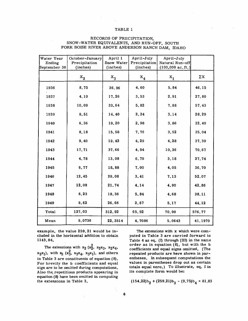
TABLE 1

RECORDS OF PRECIPITATION, SNOW-WATER EQUIVALENTS, AND RUN-OFF, SOUTH

FORK BOISE RIVER ABOVE ANDERSON RANCH DAM, IDAHO

Wat~r Year October-January April1 Ending Precipitation Snow Water

September 30 (inches) (inches)

x2 x3

1.936 8.75 26.96

1937 4.10 17.26

1938 10.09 33.64

1939 8.51 14.40

1940 6.36 19.20

1941 8.18 15.58

1942 9~40 19.42

1943 17.71 37 .• 66

1944 4.78 13.08

1945 6.77 18 .. 88

1946 12.45 29.08

1947 12.08 21.74

1948 8.23 19.36

1949 9.62 26.66

Total 127.03 312.92

Mean 9.0736 22.3514

example, the value 259.21 would be in­cluded in the horizontal addition to obtain 1143.04.

The extensions with x2 (x~, x2x3, x2x4,

x2x1), with :XS (x~, x3x4, x3x1), and others

in Table 3 are constituents of equation ( 8). For brevity the b coefficients and equal sign are to be omitted during computations. Also the. repetitious products appearing in equation (8) have been omitted in computing the extensions in Table 3.

6

April-July April-July Precipitation Natural Run-off

(inches) ( 100,000 ac. ff.)

x4 x1 :rx

4.60 5.84 46.15

3.53 2,91 27.80

5.82 7.88 57.43

2.24 3.14 28.29

2.98 3.86 32.40

7.76 3.52 35.04

4.29 4.28 37.39

4.94 10.36 70.67

6. 70 3.18 27.74

7.00 4.05 36.70

3.41 7.13 52.07

4.14 4.90 42.86

5.84 4. 68 38.11

2.67 5.17 44.12

65.92 70.90 576.77

4. 7086 5.0643 41.1979

The extensions with x which were com­puted in Table 3 are carried forward to Table 4 as eq. (I) through (III) in the same order as in equation (8), but with the b coefficients and equal signs omitted. (The repeated products are here shown in par­entheses. In subsequent computations the values in parentheses drop out as certain totals equal zero.) To illustrate, eq. I in its complete form would be:

(154.22)b2 + (259.21)b3 - (9. 75)b4 = 81.83

Extensions with X2

x2 2 x2x3 x2x4 x2x1

1936 76.56 235.90 40.25 51.10

1937 16.81 70.77 14.47 11.93

1938 101.81 339.43 58.72 79.51

1939 72.42 122.54 19.06 26.72

1940 40.45 122.11 18.95 24.55 -:J

1941 66.91 127.44 63.48 28.79

1942 88.36 182.55 40.33 40.23

1943 313.64 666.96 87.49 183.48

1944 22.85 62.52 32.03 15.20

1945 45.83 127.82 47.39 27.42

1946 155.00 362.05 42.45 88.77

1947 145.93 262.62 50.01 59.19

1948 67.73 159.33 48.06 38 .. 52

1949 92.54 256.47 25.69 49.74

Totals 1306.84 3098.51 588.38 725.15

TABLE 2 EXTENSIONS OF DATA FROM; TABLE 1

(Products and Product Sums)

Check Check Sum Extensions with X3 Sum

x 2LX: x2 3 x3x4 x3x1 X 3D{

403.81 726.84 124.02 157.45 1244.20

113.98 297.91 60.93 50.23 479.83

579.47 1131.65 195.78 265.08 1931.95

240.75 207.36 32.26 45.22 407.38

206.06 368.64 57.22 74.11 622.08

286.62 242.74 120.90 54.84 545.92

351.47 377.14 83.31 83.12 726.11

1251.57 1418.28 186.04 390.16 2661.43

132.60 171.09 87.64 41.59 362.84

248.46 356.45 132.16 76.46 692.90

648.27 845.65 99.16 207.34 1514.20

517.75 472.63 90.00 106.53 931.78

313.64 374.81 113.06 90 .• 60 737.81

424.43 710.76 71.18 137.83 1176.24

5718.88 7701.95 1453.66 1780.56 14034.68

Ex ten-Extensions Check sions Check

with x 4 Sum with x 1 Sum

x2 4 x4x1 X42X. x2

1 X!"i.X

21.16 26.86 212.29 34.11 269.52

12.46 10.27 98.13 8.47 80.90

33.87 45.86 334.24 62.09 452.55

5.02 7-.03 63.37 9.86 88.83

8.88 11.50 96.55 14.90 12 5. 06

60.22 27.32 271.91 12.39 123.34

18.40 18.36 160.40 18.32 160.03

24.40 51.18 349.11 107.33 732.14

44.89 21.31 185.86 10.11 88.21

49.00 28.35 256.90 16.40 148.64

11.63 24.31 177.56 50.84 371.26

17.14 20.29 177.44 24.01 210.01

34.11 27 0 33 222.56 21.90 178.35

7 0 13 13. flO 117.80 26.73 228.10

348.31 333.77 2724.12 417 .• 46 3256.94

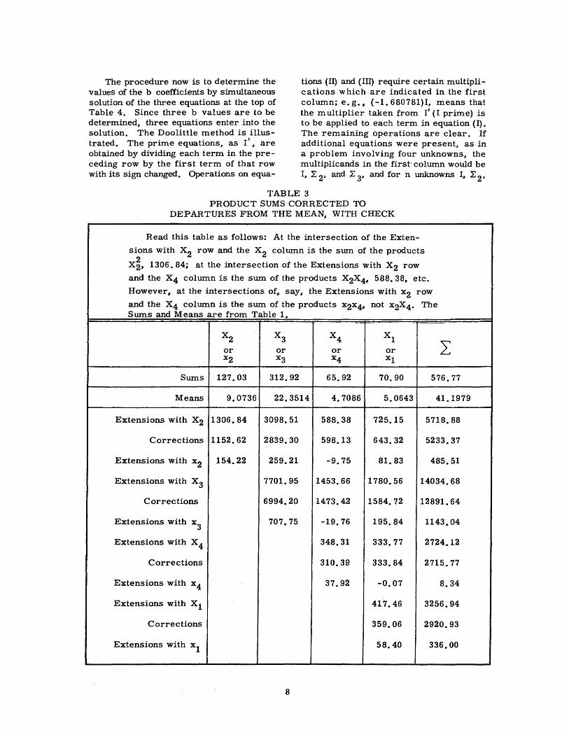
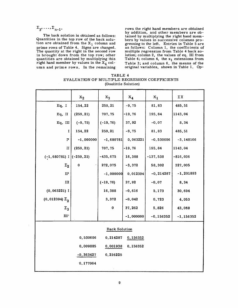
The procedure now is to determine the values of the b coefficients by simultaneous solution of the three equations at the top of Table 4. Since three b values are to be determined~ three equations enter into the solution. The Doolittle method is illus­trated. The prime equations, as I'~ are obtained by dividing each term in the pre­ceding row by the first term of that row with its sign changed. Operations on equa-

tions (II) and (III) require certain multipli­cations which are indicated in the first column; e. g., ( -1. 680781)I, means that the multiplier taken from I' (I prime) is to be applied to each term in equation (I). The remaining operations are clear. If additional equations were present~ as in a problem involving four unknowns, the multiplicands in the first" column would be I~ 2: 2, and ? 3, and for n unknowns I~ 2: 2,

TABLE 3 PRODUCT SUMS CORRECTED TO

DEPARTURES FROM THE MEAN, WITH CHECK

Read this table as follows: At the intersection of the Exten-

sions with x 2 row and the x 2 column is the sum of the products

X~, 1306. 84; at the intersection of the Extensions with X2 row

and the x4 column is the sum of the products x2x4, 588. 38, etc.

However, at the intersections of, say, the Extensions with x 2 row

and the X4 column is the sum of the products x2x4, not x 2x 4 • The Sums and Means are from Table 1.

x2 x3 x4 x1

I or or or or x2 x3 x4 x1

Sums 127.03 312.92 65.92 70.90 576.77

Means 9.0736 22.3514 4.7086 5.0643 41.1979

Extensions with X2 1306.84 3098.51 588.38 725.15 5718.88

Corrections 1152.62 2839.30 598.13 643.32 5233.37

Extensions with x 2 154.22 259.21 -9.75 81.83 485.51

Extensions with X 3 7701.95 1453.66 1780.56 14034.68

Corrections 6994.20 1473.42 1584.72 12891.64

Extensions with x3

707. 75 -19.76 195.84 1143.04

Extensions with X 4 348.31 333.77 2724.12

Corrections 310.39 333.84 2715.77

Extensions with x 4 37.92 -0.07 8.34

Extensions with x 1 417.46 3256.94

Corrections 359.06 2920.93

Extensions with x1 58.40 336.00

8

z:3, ... , z: 1 n- •

The back solution is obtained as follows: Quantities in the top row of the back solu­tion are obtained from the X 1 column and prime rows of Table 4. Signs are changed. The quantity at the right in the second row is brought down from the top row; other quantities are obtained by multiplying this right hand member by values in the x 4 col-umn and prime rows. In the remaining

rows the right hand members are obtained by addition, and other members are ob­tained by multiplying the right hand mem­hers by values in successive columns pro­gressing to the left. Entries in Table 5 are as follows: Column 1, the coefficients of multiple regression from Table 4 back so­lution; column 2, the values of eq. III from Table 4; column 4, the x 1 extensions from Table 3; and column 6, the means of the or-iginal variables. shown in Table 1. Op-

TABLE 4 EVALUATION OF MULTIPLE REGRESSION COEFFICIENTS

(Doolittle Solution)

x2 x3 x4 x1 2:X

Eq. I 154.22 259.21 -9.75 81.83 485.51

Eq. II (259. 21) 707.75 -19.76 195.84 1143.04

Eq. III (-9. 75) (-19. 76) 37.92 -0.07 8.34

I 154.22 259.21 -9.75 81.83 485.51

I' -1.000000 -1.680781 0.063221 -0.530606 -3.148166

II (259. 21) 707.75 -19.76 195.84 1143.04

(:1. 680781) I ( -259. 21) -435.675 16.388 -137.538 -816.036

2:2 0 272.075 -3.372 58.302 327.005

II' -1.000000 0.012394 -0.214287 -1.201893

III (-19. 76) 37.92 -0.07 8.34

(0. 063221) I 16.388 -0.616 5.173 30.694

(0. 012394) 2:2 3.372 -0.042 0.723 4.053

2:3 0 37.262 5.826 43.088

III' -1.000000 -0.156352 -1.156352

Back Sol uti on

0.530606 0.214287 0.156352

0.009885 0.001938 0.156352

-0.363427 0.216225

0.177064

9

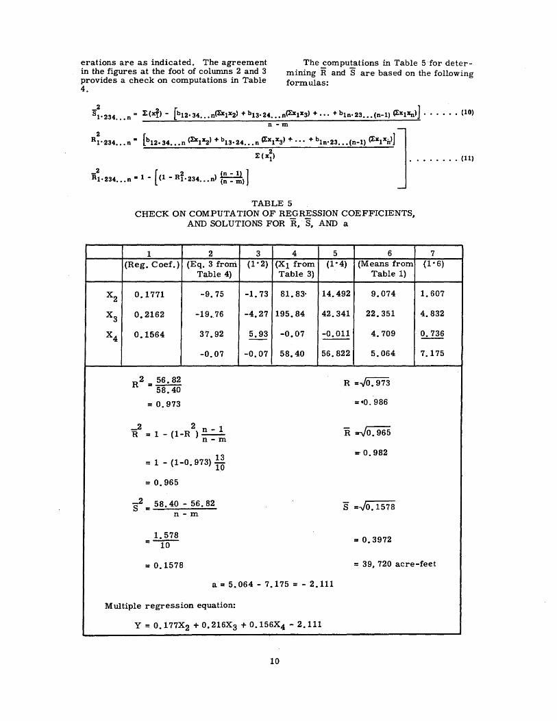
erations are as indicated. The agreement in the figures at the foot of columns 2 and 3 provides a check on computations in Table 4.

The computations in Table 5 for deter­mining R and S are based on the following formulas:

n- m

R~·-234 ••• n • [bl2•34 ••• n (l:x1~) + b13•24 ••• n ~x1x3) + •• • + b1n·23 ••• (n-1) ~x1xn>] 2

~(xl) •••••••• (11)

R • 1 - 1 - R2• ) ~ 2 [ ] 1•234 ••• n ( 1 234 ••• n (n _ m)

TABLE 5 CHECK ON COMPUTATION OF REGRESSION COEFFICIENTS,

AND SOLUTIONS FOR R, S, AND a

1 2 3 4 5 6 (Reg. Coef.) (Eq. 3 from (1• 2) (X1 from (1•4) (Means from

Table 4) Table 3) Table 1)

x2. 0.1771 -9.75 -1.73 81. 83· 14.492 9.074

x3 0.2162 -19 •. 76 -4.27 195.84 42.341 22.351

x4 0.1564 37.92 5.93 -0.07 -0.011 4.709

-0.07 -0.07 58.40 56.822 5,064

R2 = 56.82 58.40

R =~0. 973

= o. 973 :40.986

_2 2 n- 1 R. =-J(C965 R = 1- (1-R ) --n- m

13 =- o. 982 = 1 - (1-0. 973) 1_0

= o. 965

_2 = 58. 40 - 56 • 8 2 s S =-J0.1578 n- m

1. 578 = o. 3972 =lQ

7 (1• 6)

1.607

4.832

0.736

7.175

= o. 1578 = 39, 720 acre-feet

a= 5.064- 7,175 =- 2.111

Multiple regression equation:

Y = 0.177X2 + 0. 216X3 + 0,156X4 - 2,111

10

R may be computed more directly~ how­ever~ with the equation

River at Anderson Ranch Dam:

2 R2 = 1 - (n - 1) S • • . . . . . • ( 11a)

Y = 0.177X2 + O. 216X3 + O.l56X4

-2. 111 • • • • • • . •. • • • • . ( 13) 2: x¥

The value of the constant a is deter­mined by the equation

where Y is in 100~ 000 acre-foot units. This equation is a summarizing expres­sion of the observed data.

a =M -[b M 1·234 ... n 1 12·34 ... n 2 To test the correctness of this equation~ it may be applied to climatological and run.:. off data for the period of record~ and the agreement noted between estimated run-off~ Y~ and observed run-off~ X1.

+b M +b M] 13·24 ..• n 3 1n-23 ••. (n-1) ~

• . • • ( 12~

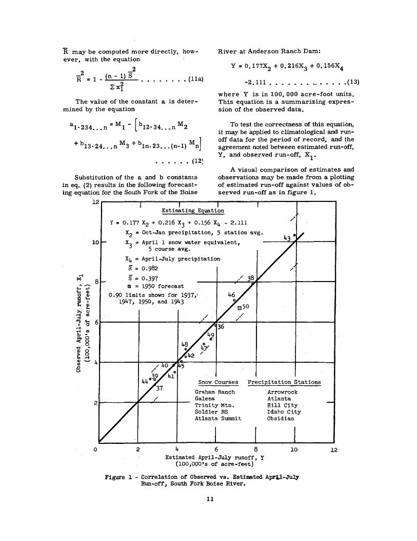
Substitution of the a and b constants in eq., (2) results in the following forecast­ing equation for the South Fork of the Boise

A visual comparison of estimates and observations may be made from a plotting of estimated run-off against values of ob­served run-off as in figure 1.

c... 0

:fl 0 0 0

"' 0 0 ...... -

12~------~--------~--------~--------,---------r-------~

Estimating Equation

Y = 0.177 x2 + 0.216 x3 + 0.156 x4 - 2.111 x2 = Oct-Jan precipitation, 5 station avg.

10 x3

= April 1 snow water equivalent, 5 course avg.

8

6

4

0

X4 = April-July precipitation

R = 0.982

s = 0.397 l!l = 1950 forecast

0.90 limits shown for 1937,: 1947, 1950, and 1943

Snow Courses Precipitation Stations

2 4

Graham Ranch Galena Trinity Mtn. Soldier RS Atlanta Slmliilit

6 8 Estimated April.:.July runoff, Y

(lOO,OOO's of acre-feet)

Arrowrock Atlanta Hill City Idaho City Obsidian

10

Figure 1 - Correlation of Observed vs. Estimated April-July R1m-of'f 1 South Fork Boise River.

11

12

X (j

0.0 0.1 0.2 0.3 0.4

0.5 0.6 0.7 0.8 0.9

1.0 1.1 1.2 1.3 1.4

1.5 1.6 1.7 1.8 1.9

2.0 2.1 2.2 2.3 2.4

2.5 2.6 2.7 2.8 2.9

3.0 3.1

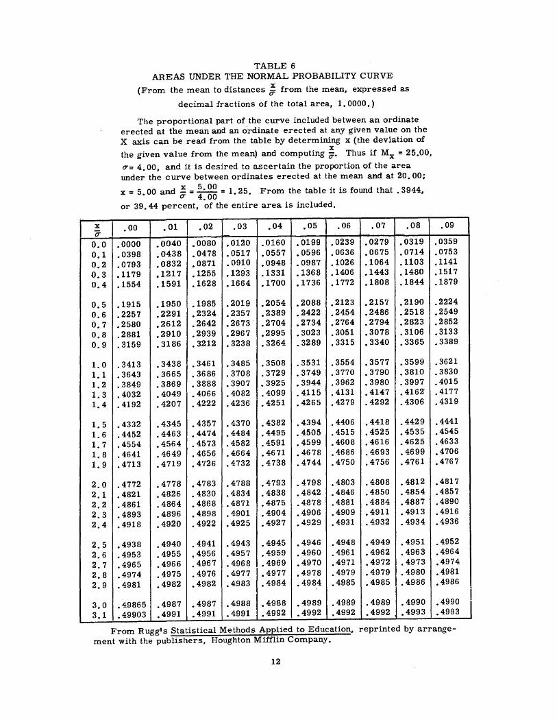
TABLE 6 AREAS UNDER THE NORMAL PROBABILITY CURVE

(From the mean to distances ~ from the mean, expressed as

decimal fractions of the total area, 1. 0000.)

The proportional part of the curve included between an ordinate erected at the mean and an ordinate erected at any given value on the X axis can be read from the table by determining x (the deviation of

the given value from the mean) and computing ~- Thus if Mx = 25.00, t:r= 4. 00, and it is desired to ascertain the proportion of the area under the curve between ordinates erected at the mean and at 20. 00;

x = 5. 00 and ~ = !: gg = 1. 25. From the table it is found that • 3944,

or 39.44 percent, of the entire area is included .

• 00 • 01 .02 .03 • 04 .05 • 06 .07 .08 ·-

.0000 .0040 • 0080 .0120 .0160 • 0199 .0239 .0279 .0319

.0398 .0438 .0478 • 0517 .0557 .0596 .0636 .0675 .0714

.0793 .0832 • 0871 .0910 .0948 .0987 .1026 .1064 .1103

.1179 .1217 .1255 .1293 .1331 .1368 .1406 .1443 .1480

.1554 .1591 .1628 .1664 .1700 .1736 .1772 .1808 .1844

.1915 .1950 .1985 .2019 .2054 .2088 .2123 .2157 .2190

.2257 .2291 .2324 .2357 .2389 .2422 .2454 .2486 .2518

.2580 .2612 .2642 .2673 .2704 .2734 .2764 .2794 .2823

.2881 .2910 .2939 .2967 .2995 .3023 .3051 .3078 .3106

.3159 • 3186 • 3212 • 3238 .3264 • 3289 .3315 .3340 .3365

.3413 .3438 .3461 .3485 .3508 .3531 .3554 .3577 .3599

.3643 .3665 • 3686 • 3708 .3729 .3749 • 3770 • 3790 .3810

.3849 .3869 .3888 • 3907 .. 3925 .3944 .3962 .3980 .3997 • 4032 .4049 • 4066 • 4082 .4099 . 4115 . 4131 .4147 • 4162 • 4192 .4207 • 4222 . 4236 • 4251 .4265 . 4279 • 4292 .4306

.4332 .4345 .4357 • 4370 • 4382 .4394 .4406 .4418 • 4429

.4452 .4463 • 4474 • 4484 .4495 • 4505 • 4515 .4525 .4535

.4554 .4564 • 4573 . 4582 .4591 .4599 • 4608 .4616 .4625

.4641 .4649 . 4656 .4664 • 4671 • 4678 .4686 .4693 • 4699

.4713 .4719 • 4726 .4732 .4738 .4744 .4750 .4756 .4761

• 4772 .4778 • 4783 .4788 .4793 .4798 .4803 .4808 • 4812

• 4821 .4826 • 4830 • 4834 .4838 • 4842 .4846 .4850 .4854

.4861 .4864 .4868 .4871 .4875 .4878 .4881 .4884 .4887

.4893 .4896 • 4898 .4901 .4904 • 4906 .4909 .4911 .4913

• 4918 • 4920 .4922 .4925 .4927 • 4929 .4931 .4932 .4934

• 4938 .4940 • 4941 • 4943 .4945 • 4946 .4948 .4949 .4951

.4953 .4955 ~ 4956 .4957 .4959 • 4960 . 4961 .4962 .4963

.4965 .4966 .4967 • 4968 .4969 .4970 .4971 • 4972 .4973

.4974 .4975 • 4976 .4977 .4977 .4978 .4979 .4979 • 4980

• 4981 .4982 • 4982 • 4983 .4984 .4984 .4985 .4985 • 4986

.49865 .4987 .4987 .4988 .4988 • 4989 .4989 .4989 .4990

.49903 .4991 .4991 .4991 .4992 .4992 .4992 .4992 .4993

• 09

.0359

.0753

.1141

.1517

.1879

.2224

.2549

.2852

.3133

.3389

.3621

.3830

.4015

. 4177

.4319

.4441

.4545

.4633

.4706 • 4767

• 4817 .4857 .4890 .4916 .4936

.4952

.4964

.4974

.4981 • 4986

.4990

.4993

From Rugg's Statistical Methods Applied to Education, reprinted by arrange­ment with the publishers. Houghton Mifflin Company.

12

I

Data on run-off season precipitation {X4 in eq. 13), are not available as of the date of forecasting. For convenience, an equation which will yield a "mean" fore­cast, subject to a calculable plus or minus error, may be obtained from eq. ( 13) by assuming normal precipitation during the run-off season. That is, by adding the product b4M 4 to the constant of eq. {i3), a new constant term is obtained, which in this example equals {0. 156) ( 4. 709) - 2. 111, or -1. 376, and the equation becomes:

Y = 0.177X2 + O. 216X3 - 1. 376 ... (13a)

As was previously mentioned, the a and b constants determined by multiple correla­tion, when employed in a forecasting equa­tion such as eq. (2), yield estimates Y which are in closest agreement with ob­served values, x1, in accordance with the th~.~ory of least squares. Owing to inac­curacies in records, inadequacies of data, etc., differences between estimates and observations are to be expected. Consider­ation must be given to the magnitude of these errors so that the investigator may know how closely the observed values of the dependent variable may be expected to approximate estimated values in future forecasts.

Estimates of errors of forecast which may be expected with given probability, taking into consideration the length of rec­ord, number of variables used, and the variation in run-off season precipitation will be treated in the following sections.

Multiple Correlation Coefficient, Standard Deviation, and Standard Error of Estimate

The coefficient of multiple correlation, R, {0. 986 in this problem), is a measure of the strength of the relationship in the sample (14 years of record) between the independent and dependent variables. A value of R equal to zero indicates no re­lationship; an R of one indicates perfect correlation. Whether a relationship be­tween any particular independent variable and the dependent variable is direct or inverse is determined by the sign of the b coefficient of that variable.

The adjusted value of the coefficient of multiple correlation, R = 0. 982, was ob­taine.d by correcting for length of record,

13

n, and for the number of constants, m {a and b 1s), which were determined (same as number of variables in the type of equa­tion used). In computing R, Table 5, the expression n-m represents the degrees of freedom. The R is an estimate of the true correlation which probably exists in a uni­verse of such data, as distinguished from the sample. It will be seen that an increase in the number of variables has the effect of reducing the estimate of the correlation in

-2 the universe. R is the coefficient of de-termination, and expresses the portion of the variance in the dependent variable which has been explained.

The standard deviation, cr, is a measure of dispersion, or scatter, of a series of items from the arithmetic mean. For a distribution of errors of estimate about a regression line the measure of dispersion is known as the standard error of estimate, S. A bar over the symbol indicates that this parameter has been adjusted for years of record and number of· variables. The use of the adjusted value, S', as well as R, is particularly important in multiple correla­tion, since in such analyses there is a tend­ency for S to be less for the sample than the true value for the universe.

The parameter, S, is expressed in units of the dependent variable and its magnitude is such that a range of plus or minus one standard error of estimate embraces about 6 8 percent of the residuals or differences between estimated and observed values. A range of plus or minus two standard errors of estimate embraces about 95 percent of all residuals. About 90 percent of the re­siduals could be expected to lie within a range of plus or minus 1. 6458. This range is limited by the 5 and 95 percentiles, the lower value of which could be expected to be equalled or exceeded 95 percent of the time; the upper value, 5 percent of the time. The probabilities mentioned above are ob­tained from tables of areas under the nor­mal probability curve (see Table 6). The ratio, jr. shown above as 1. 645 varies for small samples {under 20), and appropriate ratios for given sample sizes may be con­veniently obtained from Ezekiel's Fig. A, Appendix 3, or from Students t Table.

The standard error of the individual forecast, u Y. _ x

1• will be introduced in a

later section.

The R of 0. 982 indicates that a highly significant relationship exists, and that

about 96. 5 percent {R2

) of the variability in run-off has been accounted for; in this particular drainage basin the factors con­tributing to variations in run-off have been quite well accounted for. The S as deter­mined above will be used in determining the precision of the b coefficients (their standard deviations), and in estimating the error of the individual forecast.

Standard Deviation of Regression Coefficients

The regression coefficients as deter­mined from Tables 1 through 5 were based on a 14-year record, ·1936-1949, inclusive. Had longer records been available it is possible that the values of these coefficients would have differed somewhat from those obtained. Although the true values of the regression coefficients which would be ob­tained from a compilation of data for all time carmot be estimated, an approximation of the limits within which, for given odds, the true values might fall, can be based on the standard deviation of the computed re­gression coefficients. That is, the odds are about 68 in 100 that the true value of b

for a compilation of data for all time would lie within plus or minus one standard devi­ation of that obtained from the available data. These odds increase for multiples of the standard deviation of the regression coefficients as was previously discussed in connection with the standard error of estimate, S.

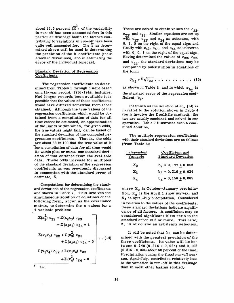
Computations for determining the stand­ard deviations of the regression coefficients are shown in Table 7. This involves the simultaneous solution of equations of the following form, known as the covariance matrix, to determine the c values for a 4-variable problem:

3

2 .l:(x2) c22 + l:(x2x3) c23

+ l: (x2x4) c24 = 1

2 l: (x2x3) c22 + l: (x3) c2 3

l: (x2x4) c22 + l: (x3x4) c2 3

2 +l: (x4) c24 = 0

Ibid.

•• ( 14)

14

These are solved to obtain values for c22 , c23, and c24• Similar equations are set up with c32, c33, and c34 as unknowns, with 0, 1, 0 on the right of the equal sign; and finally with c42, c43, and c44 as unknowns with 0, 0, 1 on the right of the equal sign. Having determined the values of c22• c33• and c 44, the standard deviations may be

computed by substitution in equations of the form

. • (15)

as shown in Table 8, and in which rr b2

is

the standard error of the regression coef­ficient, b2 .

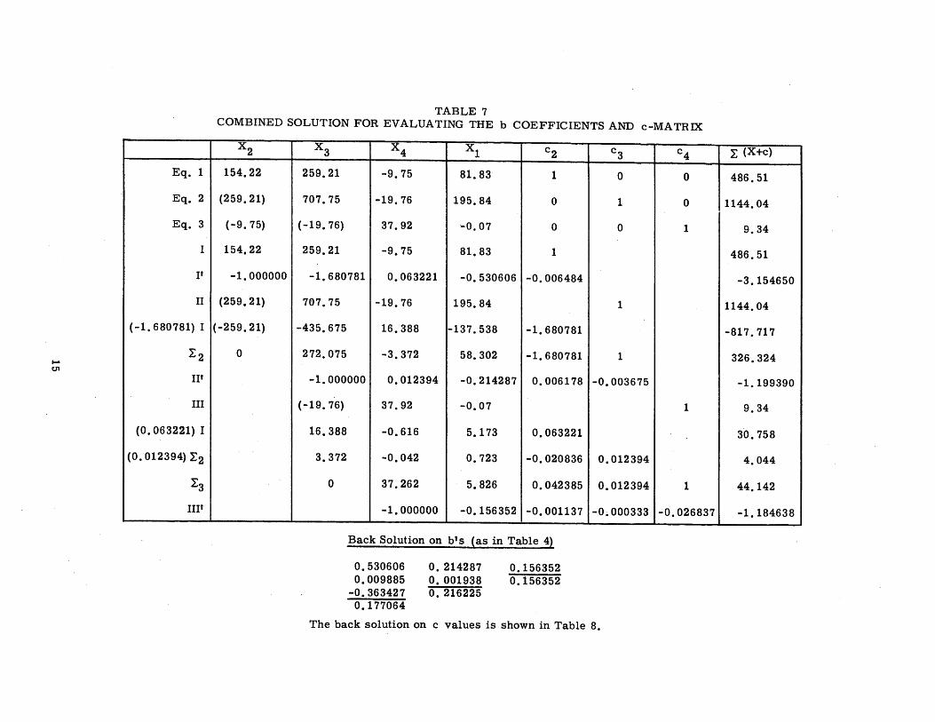
Inasmuch as the solution of eq. (14) is parallel to the solution shown in Table 4 (both involve the Doolittle method), the two are usually combined and solved in one operation. Table 7 illustrates such a com­bined solution.

The multiple regression coefficients with their standard deviations are as follows (from Table 8):

Independent Variable

Coefficient and Standard Deviation

b2 = 0.177 .± 0.052

b3 = o. 216 .± 0. 024

b4 = 0.156 .± 0.065

where x 2 is October-January precipita­tion, x3 is the April 1 snow survey, and X4 is April-July precipitation. Considered

in relation to the values of the coefficients, these standard deviations indicate signifi­cance of all factors. A coefficient may be considered significant if its ratio to the standard error is 2 or more. This ratio, 2, is of course an arbitrary selection.

It will be noted that b 3 can be deter­mined with the greatest precision of the three coefficients. Its value will lie be­tween 0. 240 (0. 216 + 0. 024) and 0.192 (0. 216 - 0. 024) about 68 percent of the time. Precipitation during the flood run-off sea­son, April-July, contributes relatively less to the varl.ation in run-off in this drainage than in m:ost other basins studied.

..... c.n

Eq. 1

Eq. 2

Eq. 3

I

I'

II

(-1. 680781) I

r2

II'

III

(0. 063221) I

(0. 012394) ~2

r3

III1

TABLE 7 COMBINED SOLUTION FOR EVALUATING THE b COEFFICIENTS AND c-MATRIX

x2

154.22

(259. 21)

( -9. 75)

154.22

-1.000000

(259. 21)

(-259.21)

0

x3 x4 x1 c2

259.21 -9.75 81.83 1

707.75 -19.76 195.84 0

( -19. 76) 37.92 -0.07 0

259.21 -9.75 81.83 1

-1.680781 0.063221 -0.530606 -0.006484

707.75 -19.76 195.84

-435.675 16.388 -137.538 -1.680781

272.075 -3.372 58.302 -1.680781

-1.000000 0.012394 -0.214287 0.006178

(-19. 76)

16.388

3.372

0

37.92 -0.07

-0.616 5.173 0.063221

-0.042 0.723 -0.020836

37.262 5.826 0.042385

-1.000000 -0.156352 -0.001137

Back Solution on b's (as in Table 4)

0.530606 0.009885

-0.363427 0.177064

o. 214287 o. 001938 o. 216225

0.156352 0.156352

c3

0

1

0

1

1

-0.003675

0.012394

0.012394

-0.000333

The back solution on c values is shown in Table 8.

c4

0

0

1

1

1

-0.026837

~ (X+c)

486.51

1144.04

9.34

486.51

-3.154650

1144.04

-817.717

326.324

-1.199390

9.34

30. 758

4.044

44.142

-1.184638

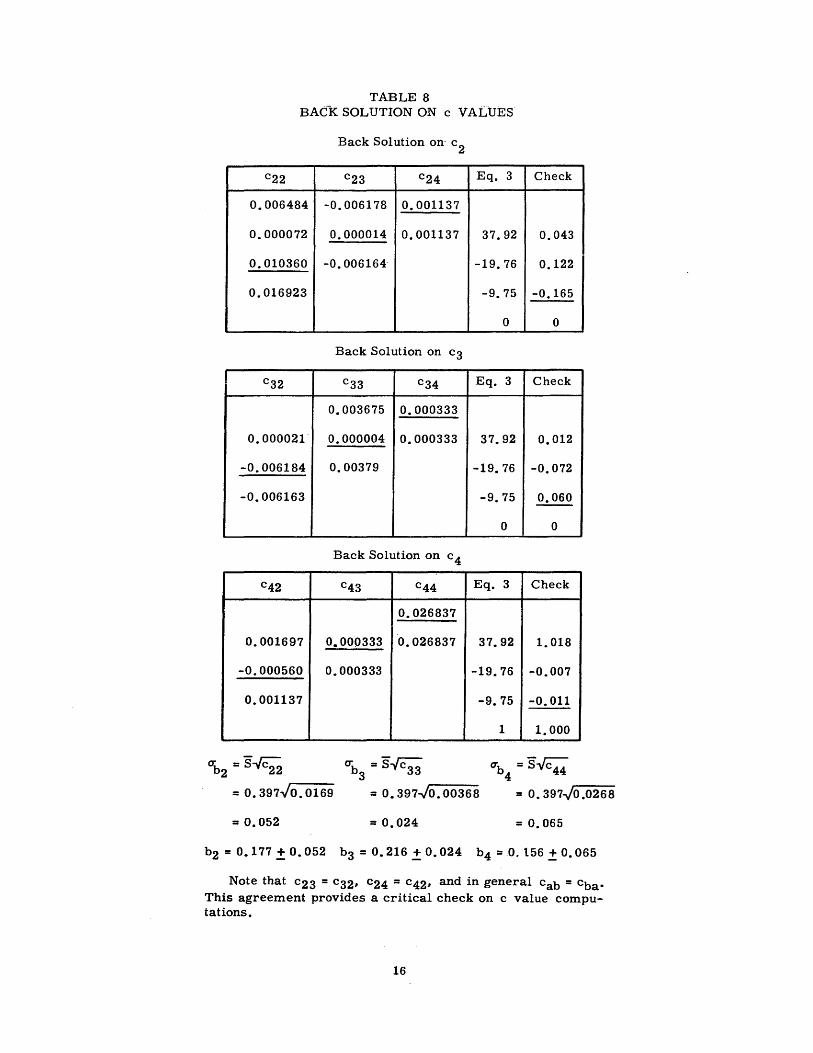
TABLE 8 BACK SOLUTION ON c VALUES

c22

0.006484

0.000072

0.010g6o

0.01692g

I cg2

0.000021

-0.006184

-0.00616g

c42

0.001697

-0.000560

0.0011g7

CTb =S~ 2 .

Back Sol uti on on· c 2

c2g c24

-0.006178 0.0011g7

0.000014 0.0011g7

-0.006164

Back Solution on cg

egg cg4

o.oog675 o.ooo3gg

0.000004 o.oooggg

o.oog79

Back Solution on c 4

c4g c44

0.0268g7

o.oooggg 0.0268g7

o.oooggg

crb = S""cgg g

Eq. g Check

g7.92 0.043

-19.76 0.122

-9.75 -0.165

0 0

Eq. 3 Check

g7.92 0.012

-19. 76 -0.072

-9.75 0.060

0 0

Eq. g Check

g7.92 1. 018

-19.76 -0.007

-9.75 -0.011

1 1.000

ub = s-Jc 44 4

= 0. g97~,....0-. 0_1_6_9 = o. g97-Jo. oog68 = o. g97-v'0.0268

= o. 052 = o. 024 = o. 065

b2 = 0.177 ± o. 052 bg = o. 216 .± o. 024 b4 = 0. 156 ± o. 065

Note that c2g = cg2~ c24 = c42~ and in general cab = cba· This agreement provides a critical check on c value compu­tations.

16

The coefficients of multiple regression in eq. ( 13) provide information as to the average contribution of the various factors to the variation in run-off from the South Fork of the Boise River. For a change of 1 inch of precipitation accumulated during the months of October through January, an average change of 17, 700 acre-feet of run­off occurs during the subsequent flood pe­riod, April through July. Each inch of snow-water equivalent as of April 1 con-

. tributes an average of 21, 600 acre-feet to the flood season run-off; each inch of pre­cipitation during the flood season contrib­utes 15, 600 acre-feet. The constant term, a, is not to be interpreted as having any hydrologic significance.

The run-off volume indicated by the estimating equation is subject to error of forecast; a statement regarding the error to be expeGted with given probability is an integral part of the forecast. Methods of computing these limits are discussed in the. following section.

Limits of Error Related to Run-off Season Precipitation

In regions where the run-off season precipitation is an important factor con­tributing to variations in seasonal run-off, as is often the case, .the effect of this pre­cipitation is related to the error of fore­cast to be expected with any specified prob­ability.

Since the April-July precipitation is unknown on April 1, the date of run-off forecasting, certain values of this unknown will be assumed as normal or as depar:­tures ·from normal to be expected with given probability. Substitution of the nor­mal, or average, precipitation would pro­vide a mean forecast. Other values for this unknown independent variable may be assumed and the corresponding limits of error computed. For example, it may be desired to estimate the magnitude of the error of forecast which will be equalled or exceeded 5 percent of the time in a posi-

tive direction (or 5 percent of the time in a negative direction, as interests may die­tate). The probability that the error of forecast will lie within these limits ( 5 to 95_.percentile range) is 0. 90.

The_desired limits of error of forecast should include the residual inherent in the correlation along with that which would re­sult from a departure from mean run-off season precipitation. The inclusion of run-off season precipitation as an inde­pendent variable, although important in the analysis, presents a unique problem in determining the limits of error of the forecast. A method of estimating the com­bined error of forecast will be treated in the following section.

Reliability of the Individual Forecast

The accuracy of a forecast can be ex­pected to be greatest for normal values of the several variables. Errors of fore-cast increase as the values of the variables depart in either direction from their re­spective means. This is a result of com­bined errors in the mean and in the slope of the regression line, or plane. Errors in the mean displace the regression plane vertically, while errors in slope, with elevation determined by the mean, tend to widen the range above and below the mean.

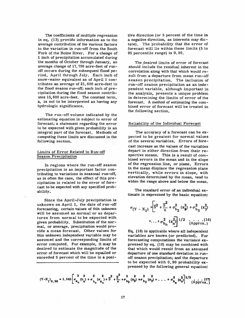
The standard error of an individual es­timate is expressed by the basic equation:

• . . . (16) (Approx.)

Eq. (16) is applicable where all independent variables are known (or predicted). For forecasting computations the variance ex­pressed by eq. (16) may be combined with that which would result from an assumed departure of one standard deviation in run­off season precipitation; and the departure to be expected with 0. 90 probability ex­pressed by the following general equation:

[ 2 2 2 2 _2 52

2 . 2 2 2 2 2~1/2 (Y-X1)0 go • 1. 645 CT (b ) + CTb (u ) + S +- +CTb (;) +ub (x3) + ••• + trb (X ) ••• (17)

• Xu u u xu n 2 3 n n (Approx.)

17

where

(Y ... X1>o. 90 = error of individual forecast which would be exceeded on the average one time in ten in either a plus or minus sense,

S = st~ndard error of estimate for an equation such as (13) in wh1ch run-off season precipitation was included in its derivation,

0h2

, ub3

., ••• , CTb = standard errors of multiple regression coefficient c;;f n known variables for an equation including run-off season

precipitation.,

x2, x3, ••• , Xn =departures from mean for known variables,

CTxu = standard deviation of run-off season precipitation (u for unknown),

~ = standard error of regression coefficient for run-off u season precipitation, and·

bu = regression coefficient of run-off season precipitation.

Note that run-off season precipitation, xu, is treated in the first two terms of this equation, and is not included in the series. The st~ndard deviation of xu, may be determ1ned by the general ex­pression

ux ~jg · . · ......... (18)

An equivalent expression for the standard deviation is

{};x2- nM2 O"x = n - 1 x • • • • • • • • • ( 18a)

Eq. (18a) obviates the need for comput­ing the departures from the mean, X - M = x. for each year of record. Substituting in eq. (18) or (18a) the standard deviation of X4 for the South Fork of the Boise River problem is

~ 3

, or + 1. 708 inches.

(In most basins fairly long records of pre­cipitation are available for determining the standard deviation of this variable.) About 68 percent of the time the April­July precipitation, x 4, may be expected to lie within a range 1. 708 inches above or below the mean value, i.e., within a range of 4. 71 + 1. 708. (A distribution of total precipitation for a period of months,

18

such as April through July, usually shows no appreciable departure from the normal. Therefore, asymmetric distribution will not be considered in this discussion.)

The error of forecast for given prob­ability will vary from year to year .depend­ing upon the magnitude of departures from normal of the various independent vari­ables. The error must, then., be com­puted for each forecast. To facilitate the computations the terms of equation (17) may be considered in two groups. Group one., the first four terms .within the brack­ets., contains quantities which remain con­stant from year to year. Group two, em­bracing the remaining terms within the bracket, contains terms which have to be evaluated for each year. The terms of group one are evaluated below, for future reference, for the South Fork Boise River problem:

2 s = = 0.1578 •

--2 s 0.1578 = 0 .. 0113 -= n 14

2 2 ub

4 (ux

4) = (0.065)2 (1.708)2 = 0.0123

2 2 b4 (ux

4> = (0.156)

2 (1. 708)2 = 0.0710

Total = 0.2524

Application of eq. ( 1 7) will be illustrated~ using data for the 1950 flood season~ South Fork Boise River Basin.

Computations for the April 1~ 1950 Forecast~ with 0. 90 Limits of Error

Pertinent records of precipitation and snow-water equivalents for the April 1~ 1950 forecast of April-July run-off are:

x2 (observed October -through-January accumulated precipitation~ average of five stations) = 10.44 inches;

x 3 (observed April1 snow-water equiv­alent~ average of five courses) = 31. 00 inches.

A mean forecast~ obtained by substi­tuting the above values in eq. (13a) is as follows:

0. 177 X 10. 44 = 1. B7

0. 216 X 31. 00 = 6. 70

Constant term~ a= -1.38

Total = 7.19 (100~000 acre-foot units)

The 0. 90 probability limits of error are computed as follows:

Values required for substitution in eq. (17) are:

x2 = x 2 - M 2 = 1 o. 44 - 9. o 7

= 1. 37,

x 3 =X3 -M 3 = 31.00-22.35

= B. 65,

062 = o. 052,

(Tb3 = o. 024,

(Tb4 = 0. 065,

2 s = 0.157B,

<TX4 = 1. 708 J

19

where M2 and M 3 are from Table 1; <Tb ~ -22

<Tb3 ~ and <T b4

are from Table B; and S is

from Table 5. The 0. 90 limits· of error for the 1950 forecast are

· (Y -X1)o. 90 = 1. 645 [ 0. 2524*

2 2 2 2 + O'h (x2) + O"b (x3) 2 3

= 1. 645 [ o. 2524

+ (0. 052) 2(1. 37) 2

+ (0. 024) 2(8. 65)2]1/2

= ± 0. 900 (100,000 ac. ft. units)

The anticipated April-July run-off for 1950 would be expected, with 0. 90 prob­ability, to fall between 7.19 + 0. 90 = B. 09, and 7.19 - 0. 90 = 6. 29. Or~ expressed in another way, for-I'950 conditions, the run-off would be expected to equal or ex­ceed 8. 09 about 5 percent of the time and to equal or exceed 6. 29 about 95 percent of the time, all in 100, 000 acre-foot units.

The 1950 forecast is plotted against observed run -off in fig. 1. Also shown on fig. 1 are the 0. 90 probability limits for a normal year, 194 7; for the high year.. 1943; and for a low year, 1937. All are based on eq. (17).

Inspection of eq. (17) will make clear certain characteristics of limits of error of the forecast. For example~ the relative departures x of the respective independent variables· from their means, will vary from year to year~ indicating a different magni­tude of error for each year~ even for years of equal run-off. Also~ it is apparent that as these departures {x' s) increase, either in a plus or minus direction, the error of forecast may be expected to increase. Fur­thermore, an increase in the standard devi­ation of the regression coefficients (<rb val­ues), indicates an increase in the error of forecast. This will explain a need for com­puting the standard error of the regression coefficients, and for eliminating any non­significant factors.

-2 *This term combines the 52. L. b~ (~ _ _), cr~ <a! ) terms

n -u u u of equation (1 7) as discussed in the preceding section.

CHARACTERISTICS OF LIMITS OF ERROR FOR TWO TYPES OF

FORECASTING EQUATION

Eq. (13a), described in the preceding pages, was obtained from a basic eq. (13) in which the run-off season precipitation was considered.

Instead of eq. (13a)~ a biased forecast­ing equation could have been derived by means of a multiple correlation involving only the x2 and x3 variables in relation to run-off, thus neglecting the effect of the x 4 variable and its influence on the remaining regression coefficients. Such an equation for the South Fork of the Boise River is as follows (computations not shown):

Y = 0.110 x 2 + o.214 x 3 - 1.273

(biased equation)

Owing to the high correlation between run­off and related factors in the South Fork of the Boise River Basin and to the rela­tively small effect and low significance of run-off season precipitation in this area the two equations do not differ significantly; however, a comparison of results will il­lustrate certain typical characteristics of the two equations. Of particular interest is a comparison of errors of forecast. (The omission of an important independent variable would introduce bias in the re­sults, and for this reason it is preferable to avoid this practice. However~ the prac­tice of neglecting the effect of run-off sea­son precipitation is a possible approach, and the results are worth considering).

Following are the multiple regression coefficients and the standard errors of these coefficients, for eq. (13a) and for the biased equation:

Biased Equation ( 13a) Equation

b2 0.17"7+0.052 0.170 + o. 062

b3 o. 216 + 0. 024 0.214,! 0.029

For the biased equation the standard error of estimate, S, equals 0. 475. The

20

variance in the estimate for this equation~ in which all independent variables are known~ would be expressed by eq. (16). Limits of error for 0. 90 probability for the 1950 season are:

1. 645 [ o. 2261 + 0

• ~!61 + (0. 062)2 (1. 37)2

+ (0. 029) 2(8. 65) 2 ] 1/ 2

= o. 919

The following is a comparison of 0. 90 limits of error for the two equations com­puted for years of different run-off poten­tialities (in 100~ 000 acre-foot units):

Equation Biased (13a) Equation

1943 (high year) 1. 27 1. 39

1950 (forecast year). 0.90 0.92

1947 (average year) 0.87 0.87

1937 (low year) 0.95 0.97

_ It is important to note that although the S for eq. (13a) is about the same in this problem as that for the biased equation (0. 477 as compared with 0. 475)~ the erroP of forecast is less for eq. ( 13a). This is the result of the smaller errors in the re­gression coefficients of eq. (13a). For the same reason the errors of forecast increase less rapidly with departures from normal conditions for eq. ( 13a) .

For the above comparison the standard error of estimate for eq. ( 13a) was com­puted from the expression

where Z is the residual, or difference be­tween estimated and observed run-off. The (J'Z is expressed by

2 LZ2 (jz = --n-

s b . . LZ 2 . ( 19) . u sbtuhng --n- 1n eq. g1ves

-~·z2 S= --n- m

In this comparison, equations (13a) and the biased equation do not differ signifi­cantly. In regions where the run-off season precipitation is a more important factor, the differences in errors of forecast for the two equations becomes more pronounced, and in abnormal years the errors are

greater for the biased equation. An addi­tional comparison of two such equations involving Colorado River data is contained in a later section.

If the values of the x 4 variable were known (or predicted) then estimates of run­off based on eq. (13) would be subject to errors of forecast determined by eq. (16). These errors, for 0. 90 probability, would be as follows for a high, an average, and a low year (in 100, 000 acre-foot units):

Error for high year (1943) = + 1.17

Error for average year (1947) = + 0. 73

Error for low year (1937) = + 0.83

PRACTICAL CONSIDERATIONS PERTAINING TO

CORRELATION ANALYSES

Precision of Multiple Regression Coefficients

The precision with which a particular multiple regression coefficient can be de­termined in any analysis is a function of parameters among which are the magni­tude of the standard error of estimate, and of the correlation between that vari­able and the remaining independent vari­ables. This relationship for b2 is ex­pressed by the following formula from page 322 of Methods of Correlation Anal­ysis, by Ezekiel:

Ob = 2

_2 s

1•234 ••• n

n<{ (1-R~"34 .•• n) •••.. (20)

Significance of the b2 coefficient increases (its standard deviation decreases) as S be­comes smaller and as the indicated cor­relation between independent variables de­creases. This requirement for a low value of S would indicate the need for consider­ing all major factol'!S influencing stream flow, and will explain the presence of pre­cipitation during the flood season in the analysis for the derivation of forecasting equations in regions where. this factor is

21

an important contributor to variations in flood season run-off. Short periods of ·record accentuate the importance of close relationships between estimated and ob­served events, as expressed by the ad­i_usted coefficient of multiple correlation, R, and adjusted standard error of esti­mate, S.

Significance of Difference Between Correlation Coefficients

In the selection of the better of two or more forecasting procedures, a mechan­ical procedure would consist of trying sev­eral combinations of independent variables affecting run-off and of selecting the best combination as determined by the highest coefficient of multiple correlation. As a basic analytical procedure such an em-­pirical, trial-and-error method is to be discouraged. (A short-cut procedure for screening variables is described later.)

Certain reservations are in order in following out this empirical procedure. That is, the difference in the correlation coefficients, R, must be significant if the conclusion as to the best combination is to have a real meaning. For if the difference in R 1s is subject to chance occurrence, then the selection of variables based on

differences in R 1 s is likewise a matter of chance. Some examples of the signifi­cance of the difference between two R's when both values are in a high range (R = 0. 90 or over) as compared with the sig­nificance of the difference between two R t s ih a lower range (R = 0. 80- or lower) will provide a basis for judgment in interpret­ing results of analyses.

Consider first the range below R = 0. 80. For example, coefficients of 0. 80, or even 0. 55, are significant for n = 16 and m = 3 (13 degrees of freedo~). However, the difference between these two values of R is significant only at the 22-percent level, which means that so large a difference from chance causes may be expected about 22 times in 100. This difference· would not be considered significant. By way of comparison it is important to note that for the higher values of R the difference be­tween an R of 0. 91 and an R of 0. 98 is more significant than the far greater dif­ference between an R of 0. 80 and an R of 0. 55; it is in fact significant at the 5-per­cent level. This further illustrates the importance of high correlations to assure realistic conclusions. For lengths of hy­drologic records usually available, say 20 years, it is only when values of R are in the 0. 90 1 s that significance may be attributed to differences between two signif­icant correlations. Inclusion of flood season precipitation often contributes appreciably to this higher correlation, and, in fact, leads to the difference between significance and nonsignificance in the differences pe­tween two R's. Insignificant differences could be a matter of chance, and the ap­parent order of importance in such cases could change with added years of record. The requirement for significance of the difference should be kept in mind in se­lecting independent variables in simple or multiple correlations.4

Concerning the empirical selection of variables, it should be remembered that if the several variables are selected by considering a large number of possible independent variables, and by retaining

Corn1,11tations of significance of difference in the above examples are based on a Z transformation described in Statistical Methods for Research Workers (Revised) by R. A. Fisher, Hainer, New York, 1950; and in applied GeneralStatistics by Croxton andCowden, Prentice-Hall, New York, 1939. Charts on pages ~~6 to 50~ ?f Ezekiel's Methods of Correlation Analysis, second edll_Io_n, facili­tate the judging of the significance of correlation coefficients.

22

only those which show the highest corre­lation with the dependent variable, there is a large possibility of the correlation in the sample exceeding the true correlation in the universe. If error calculations are to be used in judging the significance of the correlations, the variables must be selected on a logical basis.

Number of Variables

Although the inclusion of major factors contributing to variation in the dependent variable is important, it is equally impor­tant that only pertinent variables be in­cluded in the analysis, keeping the num­ber of variables as low as practicable con­sistent with efficient use of data. The effect of increased numbers of variables on the apparent correlation, and the need for adjusting the coefficient of multiple correlation and the standard error of es­timate as required to correct for num­bers of variables and length of record, may be impressively demonstrated by correlat­ing random, tmrelated variables and noting the increase in the value of R and the de­crease in S with increased numbers of these unrelated variables. Results of such an example are tabulated below.

For this demonstration, a 10-year pe­riod of stream flow record was used as a dependent variable. The independent vari­ables were taken from Table 1. 2, Ten Thousand Randomly Assorted Digits, in Snedecor1s Statistical Methods, 4th Edition~ Four trials were made using 3, 4, 5, and 9 sets of random numbers as independent variables. Values obtained for R (unad­justed) for different numbers of variables are as follows:

Total number of variables

4

5

6

10

Coefficient of correlation, R

(unadjusted)

0.15

0.55

0.84

1 .. 00

5 Snedecor, George W •• Statistical Methods, Collegiate Press. Ames. Iowa. 1946.

It would appear that R increases automat­ically with m, and that for m = n (zero de­grees of freedom) the coefficient of multi­ple correlation. R. unadjusted for degrees of freedom, has a value of 1. 00. This indicates perfect correlation, for a pop­ulation in which no real relationship exists. However, the adjusted coefficient, R.. for these trials, gives no evidence that the sample was not drawn from totally unre-

--2 lated series of data. (For values of R less than zero. the R is considered to be zero.)

The foregoing example illustrates the need for considering the degrees of free­dom. The meaning of the expression. de­grees of freedom, as applied in correlation analysis. may be clarified by reasoning as follows. Suppose. for a two-variable cor­relatio~ coordinate points are plotted rep­resenting two years of record. (For two years of record and two variables the de­grees of freedom, n - m, would be zero. ) The two coordinate points would determine a line. However, with these two observa­tions there are no cases of departure from the line, and thus no basis for computing a measure of probable departures from the line. Similarly, for a three-variable re­lationship, describing a plane, three ob­servations fix the position of the plane. Only when observations exceed three are there any departures from the plane upon which to base estimates of dispersion or strength of relationship. In working with short periods of record it is especially im.­portant that the number of variables be restricted if stable results are to be ob­tained.

As demonstrated in the previous sec­tion on reliability of the individual esti­mate, the inclusion of a variable having a large value of o-b increases the expected

error of forecast for abnormal values of that variable. The requirement for sig­nificance of the various independent vari­ables automatically limits the number of variables which may be included.

Correlation Between Independent Variables

An added contributor to unstable re­sults is·high correlation between inde­pendent variables. The effect of such a

23

relationship in increasing the standard error of the regression coefficient is ex­pressed in eq. (20). A high correlation between independent variables may lead to illogical results. possibly to the extent of indicating relationships not in agreement with known physical behavior. If perfect correlation existed between two independent variables there would be no way of separ­ating the effects of each. Examples of data on causal factors which could be expected to be ciosely correlated are records from two precipitation stations or two snow courses having similar exposure. If units of measure will permit, the closely cor­related records may be combined and used as a single causal factor. Otherwise, one of the correlated variables may be dropped.

Some degree of correlation, either real or fortuitous, between independent variables is to be expected. If one of two factors so related is omitted, the factor retained will take on added weight. Whether the relationship is real or fortuitous may have a bearing on the procedure in a given analysis. · For example, if flood season precipitation were closely associated with some antecedent e~ent, as winter precipi­tat ion, then· omission of the former, al­though significantly related to run-off, might be desirable. However, probably no significant relationship exists between precipitation amounts for different seasons.

Inclusion of Run-off Season Precipitation; Revision of Forecast

In the preceding paragraphs the inclu­sion of run-off season precipitation as a means of improving reliability was con­sidered. An added practical use of this factor is that of following up the forecast with revised forecasts, as the season ad­vances and precipitation records for the earlier portions of the season become avapable. These recorded values are substituted in the equation, along with as­sumptions for the remainder of the season, and a revised forecast prepared. Through a more complete understanding of cause and effect made possible by the inclusion of all significant factors, a better oppor­tunity is afforded for determining the prop­er course of action in any given situation.

Fortunately, in many basins precipi­tation during the month of July or during

the June-July period does not contribute significantly to flood season run-off vol­ume. In such cases the precipitation for

these periods should be omitted. With this omission· the final run-off estimate is known at an earlier date.

SHORT-CUT M;ETHOD FOR SCREENING POSSIBLE

CONTRIBUTING FACTORS

In developing forecasting techniques for various basins differing in physiographic characteristics, it may be desired to ex­amine certain factors in addition to such usually dependable indices as snow-water equivalent, fall precipitation, and run-off season precipitation, which might logi­cally be expected to influence run~off to a measurable extent in a particular basin. If a number of possible factors are to be investigated, an approximate, graphical analysis would save considerable labor in cond:ucting exploratory work. For im­proved accuracy., the graphical analysis would be followed by a mathematical eval­uation of the .factors which appear, in the graphical explorations, to bear an im­portant relationship with run-off.

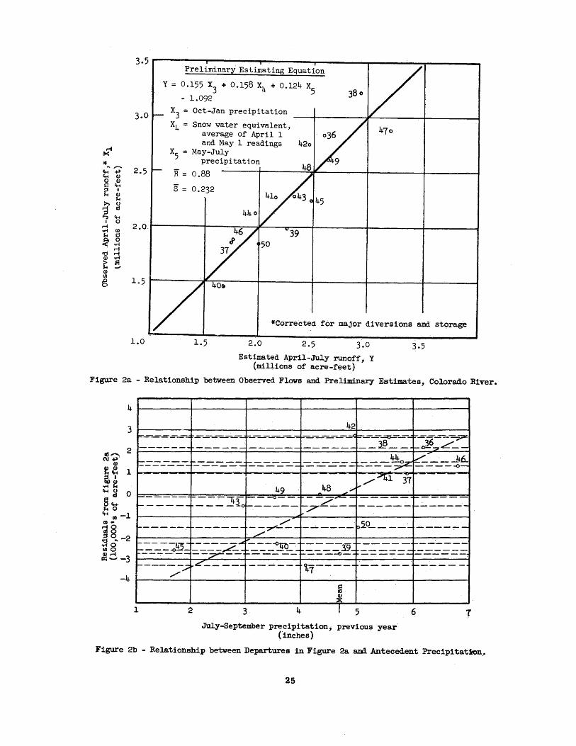
In the procedure illustrated below, the factors which are more obviously related to run-off (those which are significantly rela~­ed in most basins), are summarized in a preliminary estimating equation which is derived by methods of least squares as in the previous example. The residuals, or differences between observed run-off and estimates based on this preliminary equa­tion, are then correlated graphically with an added factor to be investigated. The following preliminary estimating equation is for the May 1 forecast of the flood season run-off, Y, in million acre-foot units, of the Colorado River at Cameo, Colorado:

Y = 0. 155X3 + 0. 158X4 + O. 124X 5 -1.092

where

x3 :!··october-January precipitation (in­ches),

x4

=snow-water equivalent (average of April 1 and May 1 surveys, inches), and

X 5 = May-July precipitation (inches).

24

Residuals, or differences between ob­served flows and estimates (fig. 2a) based on the preliminary equation are plotted in fig. 2b as ordinates against the added vari­able, precipitation during the period July through September of the previous year. The graph indicates a positive relationship between the new variable and the residuals, and hence a positive relationship between this variable and flood season run·off. Hav­ing first accounted for the effects of three important factors in the preliminary multi­ple correlation, the effect of the remaining variables becomes more clearly defined, as in fig. 2b. If in this example the new

variable had been plotted directly against run-off, it is doubtful if any relationship would have been in evidence. In such cor­relations the relationsh~p is obscured by the effects of variables not accounted for.

If additional variables which might logi­cally be expected to influence run-off are to be examined, the work will be facilitated by plotting the points for each new variable on a transparent overlay, rather thai.J. di­rectly on fig. 2b. The horizontal, dashed lines on the base figure, positioned by the residuals, are drawn to facilitate such multiple plottings. In this manner anum­ber of possible causal factors may be screened in a much shorter time than by the far more laborious trial multiple re­gressions involving various combinations of independent variables.

The graphical procedure may be ex­tended by correlating the departures from the trendline_ in fig. 2b with a second new variable, and so on. In such a series of graphs, the variables would be introduced, as far as practicable, in the order of their relative importance~

Fig. 2b could be used as a correction curve, distances from the zero residual line to be added algebraically to an estimate

.... Jl<

*"'-Ct-4 ~ Ct-4 <U 0 <U s:: Ct-4

~ • ~

~ 0

~ Ill

G-4 I 0

r-f -.'l ro J-4 s:: P4 0 < .....

r-i rd r-i <U ...... t a -<U ro

~

3.0

2.5

2.0

1.5

1.0

Preliminary Estimating Equation

Y = 0.155 x3

+ 0.158 x4 + o.l24 x5

- 1.092 x3 = Oct-Jan precipitation

x4 = Snow water equivalent, average of April l and May l readings 42o

x5 = May-July precipitation

R = o.88

s = 0.232

*Corrected for major diversions and storage

3.0 Estimated April-July runoff, Y

(millions of acre-f~et)

3.5

Figure 2a - Relationship between Observed Flows and Preliminary Estimates, Colorado River.

4 ~-------+--------~--------+---------r-------~r--------t

3

-4

42 !=--=-~-=-~ ~-= -=--=---=--~--.....:~~--=---- --= -=-~-~- :.=<F--=--=-...:::o:=- -;--,;j=":.-6-==--r-_______ _____ _: -----.------- __ 3§_- t--~-;;;;,L' __

r------r---'---...;.. ~----- ------ ___ 4}z~~--_9.n_ ------------------- -----1----- -----o-

49 -"' 48 _ ....... ~ .,.,.,~1 ·37

-- r- . 4 ~ -o - .,.,.,-- !- . . r--- ---- --- _lo-_----- _7 ____ ------ -------·-

1------.- ------ ---7'~- -~----piO ____ :_ '"""-----:---·/

1--- --4...,:--t------....:""'----oq:o-. t--- --39- 1------ t-__ :__ __ __

1------o'Z..J-----/--t-------t----- ,_ ------ -----­~----~--- --~-- 1------ r--:-----o-- ------------. r----- ---::~-~ -~ --- ------- \------ ·----- --·r-------,.,.,..,.,.,. 7

1 2 3 4 f 5

July-Septe•ber precipitation, previous year (inches)

6 r

Figure 2b - Relationship between Departures in Figure 2a and Antecedent Precipi tat:k>n .•

25

of run-off based on the preliminary formula. In this problem, however, more precise information was desired regarding the ante­cedent July-through-September precipitation as a factor influencing flood-season run-off. Therefore, a new multiple regression equa­tion was derived that included this factor. Other variables are the same as in the first equation. This new relationship is summarized as follows:

Y = 0.120X2 + 0.129X3 + 0.178X4 +0.171X5 - 1. 967

b2 = 0. 120 .±. 0. 037 (July-September precipitation, inches),

b 3 = 0. 129 .± 0. 051 (October-January precipitation, inches),

b4 = 0. 178 .±. 0. 024 (snow water, avg. of April 1 and May 1, inches), and

b = 0. 171 ± 0. 038 (May-July pre-5 cipitation, inches).

For this equation,

R = 0. 94; S = 0.169 million acre-feet.

of estimate, S, decreased from 0. 232 to 0.169 million acre-feet.

Observed vs. estimated run-off volumes are plotted in fig. 3, and the 0. 90 prob­ability limits are shown at three levels of recorded run-off: mean (1941), maximum (1938), and minimum (1940). These limits were computed by applying equation ( 1 7).

By means of such a graphical analysis as described above and illustrated in fig. 2a and 2b it was found that, in the Swan River Basin in Montana, the temperature during the snow accumulation period had a signifi­cant effect on variations in flood-season run-off. This region is frequented by warm winds during the winter months. Tempera­tures during December and March of Water Year 1934 were far above normal. The resulting snowmelt prior to the nominal flood season was evidenced in part by the occurrence on December 2 5 of the largest flood of Water Year 1934. The coefficient of multiple regression applying to tempera­ture was, in this case, negative, indicating an inverse relationship between winter temperatures and flood season run-off; i. e. , the higher the winter temperature the less the run-off during the following nominal

For all independent variables the stand- melt season. Such examples further illus-ard deviation of the regression coefficient trate the individual differences in basin is less than 1/2 the value of the coefficient, characteristics, and the need for explora-indicating significance. With the addition tory work in relating factors of cause and of the new variable, x 2, the coefficient of effect. The device illustrated in fig. 2a multiple correlation, adjusted, increased and 2b is offered as a convenient means of from 0. 88 to 0. 94, and the standard error selecting added factors in different basins.

--------------------------------------CHANGE OF DEPENDENT VARIABLE

It is sometimes required that the re­gression of different dependent variables upon the same set of independent variables be determined. For example, estimates of run-off for different periods of months or of flood volume between beginning and end of flood flow (shifting dates) may be required, or estimates of some flood flow characteristic other than total volume, such as peak flows, may be desired, based on the same independent variables. A con­venient method of analysis in such cases is described in Statistical Methods for Re­search Workers by R. A. Fisher. This method will be illustrated, using data of the Colorado River Problem. In this pro­cedure' the c values (covariance matrix) are determined, and from these the co­efficients of multiple regression are com-

26

puted from the following relationships:

b2 = c22l:(X 1 X'2) + c23l:(.X 1 X 3)

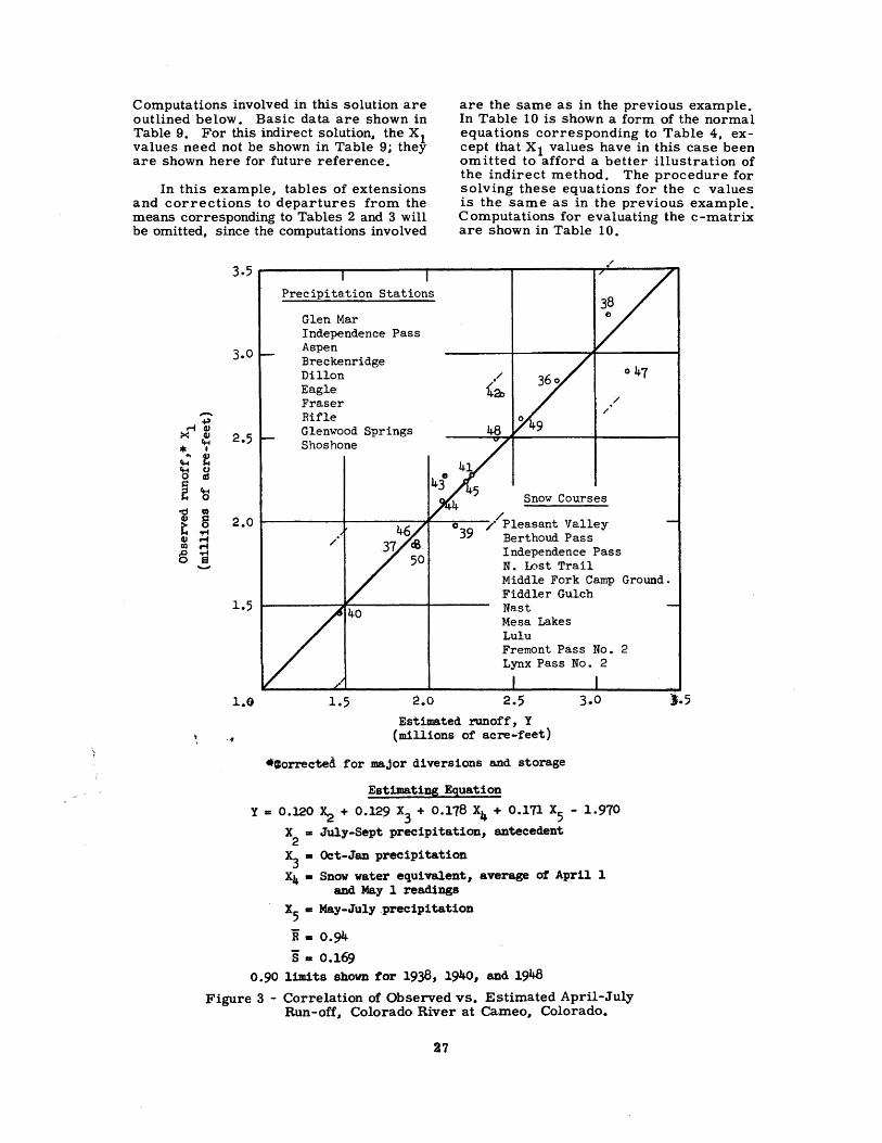
Computations involved in this solution are outlined below. Basic data are shown in Table 9. For this indirect solution, the x 1 values need not be shown in Table 9; they are shown here for future reference.

In this example, tables of extensions and corrections to departures from the means corresponding to Tables 2 and 3 will be omitted, since the computations involved

are the same as in the previous example. In Table 10 is shown a form of the norma 1 equations corresponding to Table 4, ex­cept that x 1 values have in this case been omitted to afford a better illustration of the indirect method. The procedure for solving these equations for the c values is the same as in the previous example. Computations for evaluating the c-matrix are shown in Table 10.

-~ r-fQ) >< Q)

ft-4

* ... t

ft-4 2! rg CJ

aS

e rg od Cl)

Q) 8 t .,.... Q) r-f Ul rot ~ oM a -

3.0

2.5

2.0

1.5

1.0

Precipitation Stations

Glen Mar Independence Pass Aspen Breckenridge Dillon ,/

Eagle 4a, Fraser /

Rifle /

Glenwood Springs Shoshone

Snow Courses /

/ Pleasant Valley 39 Berthoud Pass /

Independence Pass

1.5

N. Lost Trail Middle Fork Camp Fiddler Gulch Na.st Mesa Lakes Lulu Fremont Pass No. Lynx Pass No. 2

2.0 2.5 3.0 Estimated runoff, Y

(miliions of acre-feet)

•~orrected for major diversions and storage

Estimating Eguation

y = 0.120 ~ + 0.129 x3 + 0.178 x4 + 0.171 x5 - 1.970 X = July-Sept precipitation, antecedent

2 x3 = Oct-Jan precipitation

X4 • Snow water equivalent, average at April 1 and May 1 readings

x5 - May-July precipitation

'R • o.94 8. 0.169

0.90 limits shown tor 1938, 1940, and 1948

0 47

Ground-

2

Figure 3 - Correlation of Observed vs. Estimated April-July Run-off, Colorado River at Ca.meo, Colorado.

27

).5

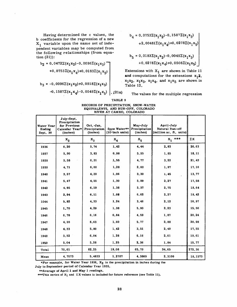
Having determined the c values, the b coefficients for the regression of a new x1 variable upon the same set of inde-

b4 = 0. 0753L(x1x2)-0.1587L(x1x3)

+2. 00481L(x1 x 4)+0. 0278L(x1 x 5)

pendent variables may be computed from the following relationships (from equa­tion (21)):

b2 = o. 0472~(xl x2) -0. 0096~(x1 x3)· ·

b5 = O.Ol83L(x1x2)-0.0049~(x1x3 )

+0. 0278L(x1 x 4)+0. 0508~(x1x5)

+0. 0753~(x1 x 4)+0. 0183L(x1 x5)

b 3 = -0. 0096~(xl x2)+0. 0918L(Xtx3)

Extensions with X 1 are shown in Table 11 and computations for the extensions x1 ~.

x1x2, x1x3. x1x4• and x1x 5 are shown in Table 12.

-o. 1587,~(x1 x 4) -0. 0049L(x1 x 5) .l21a)

TABLE 9

The values for the multiple regression

July-Sept. Precipitation

RECORDS OF PRECIPITATION, SNOW-WATER EQUIVALENTS, AND RUN-OFF, COLORADO

RIVER AT CAMEO, COLORADO

Water Year for Previous Oct. -Jan. May-July April-July Ending Calendar Year* Precipitation Snow Water** Precipitation Natural Run-off

Sept. 30 (inches) (inches) (1()::mch units) (inches) (million ac. ft. units)

x2 x3 x4 x5 x1

1936 6.20 5.74 1.42 4.44 2.83

1937 5.90 3.83 0.98 5.55 1.85

1938 5.58 6.31 .1 .. 55 4.77 3.22

1939 4.71 6.60 1.28 2.60 1.97

1940 3.57 4.39 1.06 3.30 1.45

1941 5.47 4.55 1.30 3.99 2.27

1942 4.95 6.19 1.38 3.37 2.75

1943 2.94 6.11 1.08 6.02 2.27

1044 5.82 4.33 1.24 3.46 2.12

1945 1.70 4.29 1.38 5.90 2.23

1946 6.78 6.16 0.84 4.59 1.87

1947 4.10 6.63 1.60 5.77 2.88

1948 4.33 5. 80 1.42 3.51 2.49

1949 3.52 6.04 1.28 6.16 2.61

1950 5.04 5.28 1.25 2~ 36 1. 84

Total 70.61 82.25 19.06 65.79 34.65

Mean 4.7073 5.4833 1.2707 4.3860 2.3100

*For example, for Water Year 1936, X2 is the precipitation in inches during the July to September period of Calendar Year 1935.

**Average of April! and May 1 readings. ***This series of X1 and I: X values is included for future reference (see Table 11).

28

*** ~X

20.63

18.11

21.43

17.16

13.77

17.58

18.64

18.42

16.97

15.50

20.24

20.98

17.55

19.61

15.77

272.36

18.1573

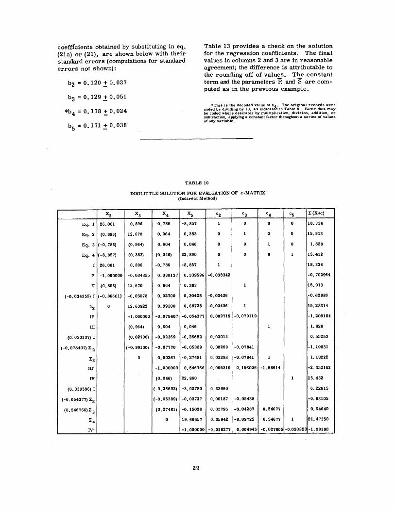
coefficients obtained by substituting in eq. (21a) or (21), are shown below with their standard errors (computations for standard errors not shown):

Table 13 provides a check on the solution for the regression coefficients. The final values in colunms 2 and 3 are in reasonable agreement; the difference is attributable to the rounding off of values. The constant term and the parameters R and S are com­puted as in the previous example.

b2 = o. 120 .± o. 037

b3 = o. 129 .± o. 051

*b4 = o. 178 :to. 024

b5 = 0.171.±0.038

x2

Eq. 1 26.081

Eq. 2 (0. 896)

Eq. 3 (-0.786)

Eq. 4 ( -8. 857)

I 26.081

I' -1.000000

II (0. 896)

( -0. 034355) I (-0. 89601)

~ 0

II'

III

(0. 030137) I

*'This is the decoded value of b4 . The original records were coded by dividing by 10, as indicatea in Table 9. Basic data may be coded where desirable by multiplication, division, addition, or subtraction, applying a constant factor throughout a series of values of any variable.

TAB~E 10

DOOLITTLE SOLUTION FOR EVALUATION OF c-MATRIX (Indirect Method)

x3 x4 x5 c2 c3 c4 c5 . l:. (X +c)

0.896 -0.786 -8.857 1 0 0 0 18.334

12.670 0.964 0.383 0 1 0 0 15.913

(0. 964) 0.604 0.046 0 0 1 0 1. 828

(0.383) (0. 046) 22.860 0 0 0 1 15.432

0.896 -0.786 -8.857 1 18.334

-0.034355 0.030137 0.339596 -0.038342 -0. 702964

12.670 0.964 0.383 1 15.913

-0.03078 0.02700 0.30428 -0.03436 -0.62986

12.63922 0.99100 0.68728 -0.03436 1 15.28314

-1.000000 -0.078407 -0.054377 o. 002719 -0.079119 -1. 209184

(0.964) 0.604 0.046 1 1.828

(0. 02700) -0.02369 -0.26692 0.03014 0.55253

( -0. 078407) l: 2 (-0. 99100) -0.07770 -0.05369 0.00269 -0.07841 -1.19831

1:3 0 0.50261 -0.27481 o. 03283 -0.07841 1 1.18222

III' -1.000000 0.546766 -0.065319 0.156006 -1.98614 -2.352162

IV (0. 046) 22.860 1 15.432

(0. 339596) I (-0.26692) -3.00780 0.33960 6.22615

(-0. 054377) l:2 (-0.05389) -o. 03737 0.00187 -0.05438 -0.83105

(0. 546766) l: 3 (0.27481) -0.15026 0.01795 -0.04287 0.54677 0.64640

l:4 0 19.66457 0.35942 -0.09725 o. 54677 1 21.47350

IV' -1.000000 -0.018277 0.004945i -0.027805 -0.050853 -1.09190

29

~ 0

c22

0.03834

0.00621

0.00227

0.00033

0.04715

C32

-0.00168

-0.00478

-0.00315

-0.00961

Back Solution on c2 ..

c23 c24 c25

-0.00272 0.06532 0.01828

-0.00099 0.00999 0.01828

-0.00590 0.07531

-0.00961

Back Solution on c3

C33 C34 C35

0.07912 -0.15600 -0.00495

0.00027 -0.00270 -0.00495

0.01244 -0.15870

0.09183

TABLE 10 (Continued)

Eq. 4 Check c42

22.860 0.418 0.00944

0.046 0.003 0.06042

0.383 -0.004 0.00545

-8.857 -0.417 0.07531

0 0

Eq. 4 Check c52

0.01727 22.860 -0.113

0.00084 0.046 -0.007

0.00017 0.383 0.035

0.01828 -8.857 0.085

0 0

Back Solution on c 4

c43 c44 c45 Eq. 4 Check

1.98961 0.02780

-0.00151 0.01520 0.02780 22.860 0.636

-0.15719 2.00481 0.046 0.092

-0.15870 0.383 -0.061

-8.857 -0.667

0 0

Back Solution on c5

c53 c54 c55 Eq. 4 Check!

0.05085 -0.00277 0.02780 0.05085 22.860 1.162

-0.00218 0.02780 0.046 0.001

-0.00495 0.383 -0.002

-8.857 -0.162

1 0.999

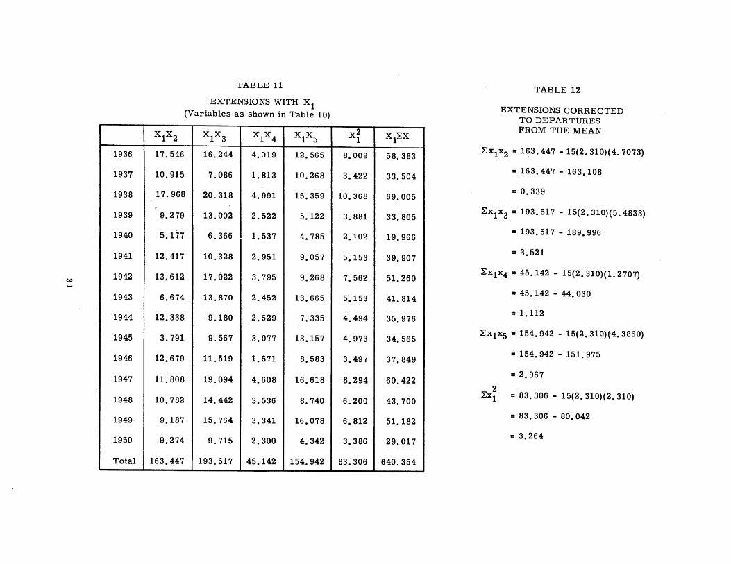
w

""""

1936

1937

1938

1939

1940

1941

1942

1943

1944

1945

1946

1947

1948

1949

1950

Total

x1x2

17.546

10.915

TABLE 11

EXTENSIONS WITH x 1 (Variables as shown in Table 10)

x1x3 x1x4 x1x5

16.244 4.019 12.565

7.086 1.813 10.268

17.968 20.31.8 4.991 15.359

9. 279 13.002 2.522 5.122

5.177 6.366 . 1.537 4.785

12.417 10.328 2.951 9.057

13.612 17.022 3.795 9.268

6.674 13.870 2.452 13.665

12.338 9.180 2.629 7 .• 335

3.791 9.567 3.077 13.157

12.679 11.519 1.571 8.583

11.808 19.094 4.608 16.618

10.782 14.442 3.536 8.740

9.187 15.764 3.341 16.078

9.274 9.715 2.300 4.342

163.447 193.517 45.142 154.942

x2 1 X12:X

8.009 58.383

3.422 33.504

10.368 69.005

3.881 33.805

2.102 19.966

5.153 39.907

7.562 51.260

5.153 41.814

4.494 35.976

4.973 34.565

3.497 37.849

8.294 60.422

6.200 43.700

6.812 51.182

3.386 29.017

83.306 640.354

TABLE 12

EXTENSIONS CORRECTED TO DEPARTURES FROM THE MEAN

LX1X2 = 163.447 - 15(2. 310)(4. 7073)

= 16 3 • 44 7 - 16 3 • 1 0 8

= o. 339

LX1X3 = 193.517 - 15(2. 310)(5. 4833)

= 193. 517 - 189. 996

= 3. 521

LX1 x4 = 45. 142 - 15(2. 310)(1. 2707)

= 45.142 - 44.030

= 1.112

LX1X5 = 154.942 - 15(2. 310)(4. 3860)

= 154. 942 - 151. 975

= 2. 967

LX~ = 83.306 - 15(2. 310)(2. 310)

= 83. 306 - 80.042

= 3. 264

x2

x3

:x4

x5

TABLE 13

CHECK ON COMPUTATION OF REGRESSION COEFFICIENTS, AND SOLUTIONS FOR R, S, AND a

1 2 3 4 5 6 (Eq. 4from (X1 from (Means from

(Reg. Coef.) Tables 10 & 12) ( 1• 2) Table 12) (1·.,4) Table 9)

0.120 -8. 857 -1.063 0.339 0.041 4.707

0.129 0.383 0.049 3.521 0.454 5.483

1.778 0.046 0 .. 082 1.112 1. 977 1. 271

0.1706 22.860 3.900 2.967 0.506 4.386 -- --2.967 2.968 3.264 2.978 2.310

R2 = 2. 978 3.264

R =.Jo. 9124

= o. 9124 = o. 955

_2 2 n-1 'R =..Jo. 878 R = 1 - (1-R )-n-m

14 = 1 - (1-0. 912)10 =- o. 937

= o. 878

_2 =3.264~2.978 s s =-Jo. 0286

n- m

0.286 = 0. 169 (169, 000 acre-feet) =--

10

= o. 0286

a= 2.310-4.277

= - 1. 967

Multiple regression equation:

Y = 0.120X2 + 0.129X3 + 0.178X4 + O. 171X5 - 1. 967

In this indirect procedure the c values serve both to determine the standard deviation of the multiple regression coefficients, and in computing the regression coefficients with equation (21).

32

7

( 1. 6)

0.565

0.707

2.257

0.748

4.277

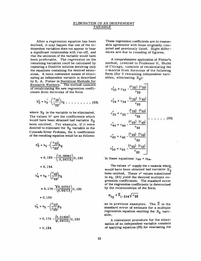
ELIMINATION OF AN INDEPENDENT VARIABLE

After a regression equation has been derived, it may happen that one of the in-:­dependent variables does not appear to bear a significant relationship with run-off, and that the omission of the variable would have been preferable. The regression on the remaining variables could be calculated by repeating a Doolittle solution involving only the equations containing the desired exten­sions. A more convenient means of elimi­nating an independent variable is described by R. A. Fisher in Statistical Methods for Research Workers. The method consists of recalculating the new regression coeffi­cients from formulas of the form

b' - b. ( c32) b 3 - 3 - c . 2 •..•••... (22) 22

where X2 is the variable to be eliminated. The values b' are the coefficients which would have been obtained had variable x 2 been omitted. For example, if it were desired to eliminate the x2 variable in the Colorado River Problem, the b coefficients of the resulting equation would be as follows:

L-o. 00961) = o. 129 -;\ o. 04715 0.120

= 0.154

1(0.00753) = o. 178 - o. 04715 o. 120

= 0. 159

= o 171 - (o. 01828)o 120 • \0.04715 •

= 0.124

33

These regression coefficients are in reason­able agreement with those originally com­puted and previously listed. Slight differ­ences are due to rounding of figures.

A comprehensive application of Fisher's method, credited to Professor H. Shultz of Chicago, consists of recalculating the c-matrix from formulas of the following form (for 3 remaining independent vari­ables, eliminating X2):

1 (C 42) (C52) c45 = c45 - ----­

c22

• (c52) (c52) c55 = c55 -

·In these equations Cab = Cba.

The values c' supply the c -matrix which would have been obtained had variable x; been omitted. These c' values substituted in eq. (21) yield the desired multiple re­gression coefficients. The standard error of the regression coefficients is determined by the relationships of the form

as in previous examples. The S is the standard error of estimate for a multiple regression equation omitting the ~ vari­able.

A convenient procedure for the elimi­nation of an independent variable consists of applying equation (22) for evaluating the

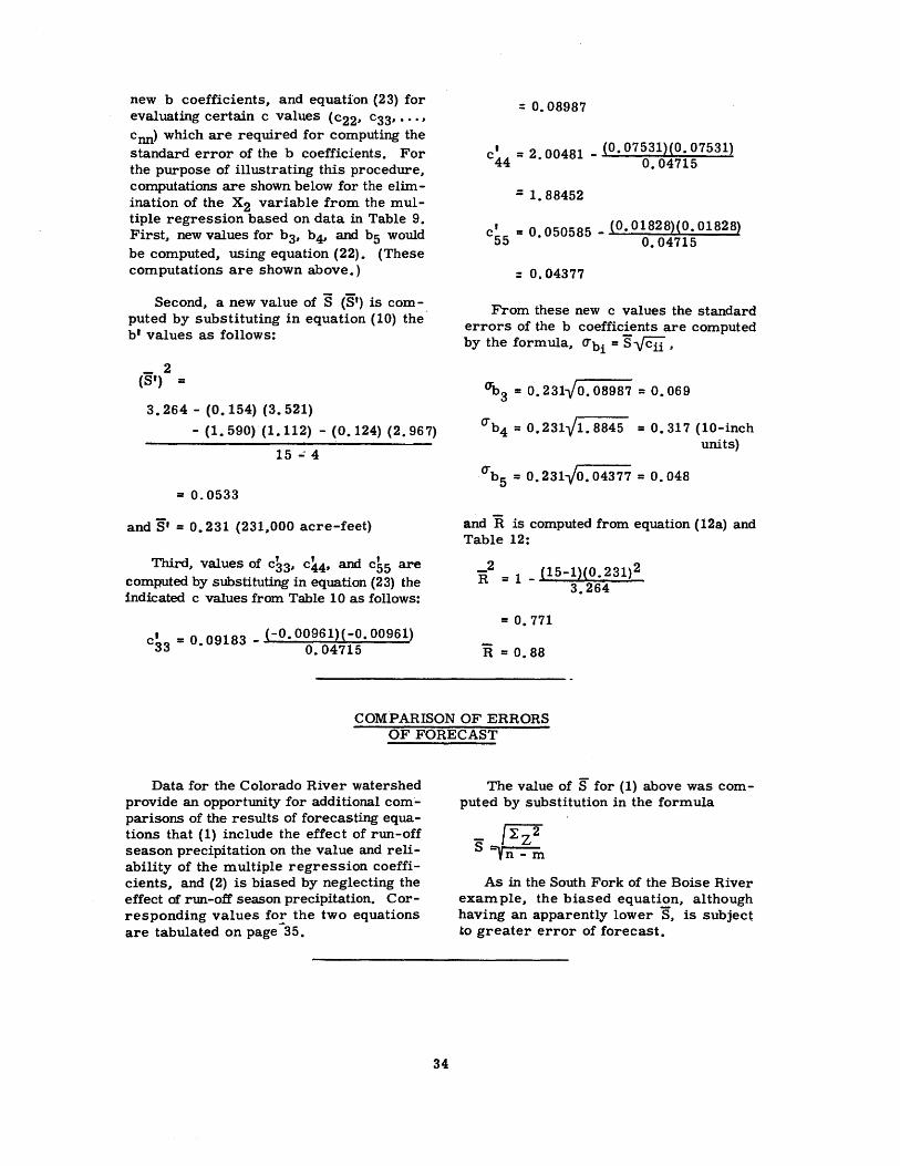
new b coefficients., and equation (23) for evaluating certain c values ( c22" c33 ..... , cnn) which are required for computing the standard error of the b coefficients. For the purpose of illustrating this procedure, computations are shown below for the elim­ination of the x2 variable from the mul­tiple regression based on data in Table 9. First., new values for b 3., b~ and b5 would be computed., using equation (22). (These computations are shown above.)

Second, a new value of S {S1) is com­puted by substituting in equation (10) the b 1 values as follows:

- 2 (S') = 3. 264 - (0. 154) {3. 521)

- {1. 590) (1. 112) - (0. 124) {2. 96 7)

15..; 4

= 0. 0533

and s• = o. 231 (231.,000 acre-feet)

Third, values of c33.. c44.. and c55 are computed by substituting in equation (23) the indicated c values from Table 10 as follows:

c' = 0 09183 _ ( -o. 00961)( -o. 00961) 33 ° 0.04715

= o. 08987

I : 2 00481 _ (0. 07531)(0. 07531) c44 · 0.04715

= 1. 88452

c' = 0 050585 _ (0. 01828)(0. 01828) 55 • 0.04715

= 0.04377

From these new c values the standard errors of the b coefficients are computed by the formula., <Tbi = S-Vcif.

<Tb3 = o. 231,jo. 08987 = o. 069

crb4 = 0.231Vl. 8845 = 0. 317 (10-inch units)

<Tb5 = 0.231-/0.04377 = 0.048

and R is computed from equation ( 12a) and Table 12:

rl = 1 _ (15-1)(0. 231)2 3.264

= o. 771

'R = o. 88

COMPARISON OF ERRORS OF FORECAST

Data for the Colorado River watershed provide an opportunity for additional com~ parisons of the results of forecasting equa­tions that (1) include the effect of run-off season precipitation on the value and reli­ability of the multiple regression coeffi­cients., and (2) is biased by neglecting the effect of run-off season precipitation. Cor­responding values for the two equations are tabulated on page~35.

34

The value of S for (1) above was com­puted by substitution in the formula

- /l;z2 S:,~

tn- m

As in the South Fork of the Boise River example., the biased equation, although having an apparently lower S, is subject to greater error of forecast.

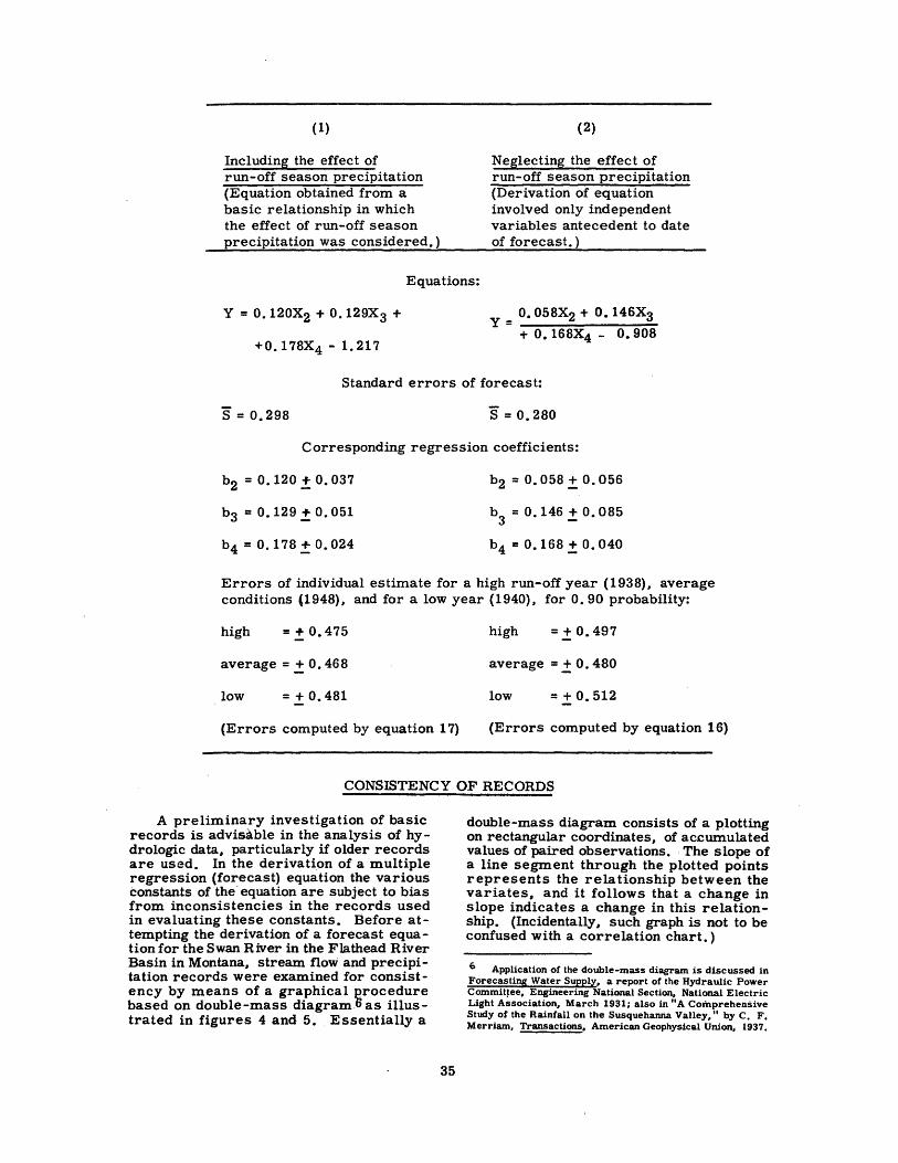
(1)

Including the effect of run-off season precipitation (Equation obtained from a basic relationship in which the effect of run-off season precipitation was considered.)

(2)

Neglecting the effect of run-off season precipitation (Derivation of equation involved only independent variables antecedent to date of forecast.)

Equations:

Y = 0.120X2 + 0.129X3 +

+ 0. 1 78X4 - 1. 217

0. 058X2 + 0. 146X3 Y=

+ 0. l68X4 - O. 908

Standard errors of forecast:

s = 0.298 s = o. 280

Corresponding regression coefficients:

b2 = o. 120 .± o. 037

b3 = o. 129 .:to. 051

b4 = o. 178 .± o. 024

b2 = o. 058:!: o. 056

b3 = o. 146 .± o. 085

b4 = o. 168.:!: o. 040

Errors of individual estimate for a high run-off year (1938L average conditions (1948), and for a low year ( 1940L for 0. 90 probability:

high = .,. o. 475 high = + 0.497

average = .± 0. 46 8 average = + 0. 480

low =.:!: o. 481 low = + o. 512

(Errors computed by equation 1 7) (Errors computed by equation 16)

CONSISTENCY OF RECORDS

A preliminary investigation of basic records is advisable in the analysis of hy­drologic data, particularly if older records are used. In the derivation of a multiple regression (forecast) equation the various constants of the· equation are subject to bias from inconsistencies in the records used in evaluating these constants. Before at­tempting the derivation of a forecast equa­tion for the Swan River in the Flathead River Basin in Montana, stream flow and precipi­tation records were examined for consist­ency by means of a graphical procedure based on double-mass diagram.B as illus­trated in figures 4 and 5. Essentially a

35

double-mass diagram consists of a plotting on rectangular coordinates, of accumulated values of paired observations. The slope of a line segment through the plotted points represents the relationship between the variates, and it follows that a change in slope indicates a change in this relation­ship. (Incidentally, such graph is not to be confused with a correlation chart.)

6 Application of the double-mass diagram is discussed in Forecasting Water Supply. a report of the Hydraulic Power Commit~ee. Engineering National Section. National Electric Light Association. March 1931; also in "A Comprehensive Study of the Rainfall on the Susquehanna Valley," by c. F. Merriam, Transactions. American Geophysical Union, 1937.

In Figure 4, accumulated values of a 7-station mean precipitation are shown as ab­scissae and accumulated precipitation re­corded at individual stations are shown as ordinates, each station having its own zero point along the vertical axis.

Of the seven precipitation stations, only the gage at Trout Creek was reported in the station histories as having been relocated. ·According to the history this gage was moved in 1930 and again in 1942.· Changes in ob­served values of precipitation· resulting from these relocations are evidenced by abrupt changes in slope of the trend line for the Trout Creek Station, figure 5. To place

·these records on a basis equivalent to that of current Trout Creek data, adjustment factors of 1 • 03 and 0. 94, respectively, were applied to the Trout Creek records obtained at the two earlier locations. Changes as small as thlS make no appreciable difference in a seven-station average, nor in the final correlation. However, such an examination

~ ., d 0 .... ~ as ~ .... PI ..... 0

2: J:lc

'd Cl) I) a ~ .... 0 ..,a .. 0 as-2! ~(I)

Cl) I)

A -'= -t (,) 0 ~~ J.t as tO·-X ...

I > J.t ..... OJ 'd .·.g s:: ~

..... 0

0

'a a T ... 0 ~ 0 as 1 j ~ •

of data is desirable, since in many series of records changes appear which are of suffi­cient magnitude to materially affect the use­fulness of the data.

The double -mass diagram in Figure 5 consists of a plotting of accumulated esti .. mates of discharges as abscissae and ac­cumulated observed discharges as ordinates. The estimates of discharge were obtained from a simple regression (not shown) of October-July runoff upon October-March precipitation .. the regression line being de­termined by records of recent years of rea­sonably consistent data. The change in the slope of the line, about 1932, in Figure 5 indicates a variation in recorded flow as related to estimated fl.ows .. or as related to precipitation. Runoff records prior to the indicated date of change in slope should be adjusted by the factor 0. 76 if they are to be considered as a part of a consistent rec­ord.

Jecarled. October-March accumulated mean precipita{,J.OD· of 7 stations

(inches)

Figure 4 - Double Mass Diagram of Precipitation Data. Individual Stations vs. Average for the Area.

36

:: ~~~~~~~~~~~~~~~~~~~~~~~~~~~--+""T"I,. ----rl-----~+--_-_-_:I~ ~~~:1 ~~~·T"~i:._--.j,!~ / __ "' =-'"~-~ 1 1 I )/[· 1927.,

Precipitation Stations I i' 1. l I~ i ~/

0 w > 0:: w (/)

m 0

13~--+----i

121---1-----l

1-----t----+---+---+-- 1\,.(o . If

Kalispell j I I ! J~~(1}2~ _j Lonepine 1---+---+--lt----' ~ .. /1'/ · , Pleasant Volley I ~,~1~9 1 j

I 1---1-----l Polson r------1--+---Hi....._~~, · i -~ St. Ignatius !l231930 1 !

1

. I 0 1931 I ! Thompson Falls , ' +. I

~ 10 1----1----1 Trout Creek . r7·1932 ! i --~-f-----l

~ 9~--~-~--~---r--~----r---+--~-~~wl~9~3333~--1-·--~l ---~ii __ -4-~ a:: u_ I I / . l I

~ § ·~--~-~---+---+---l--+---u~934 : , 1

I a::o 7~--+---~-~~-+-~--~-~~~--+---4---r---+---~--r-~ wo lA T ll III 0 1936 j

1

o..: 1--

6 ~1937 I u l 0 3e I 0 w ....... <( _J

::> :E ::> u u <(

5~--~-~--+----+ ~~~~--~---+--~--~--+----~---+--~---+-·--R.:'~y 939 i

41---+--+--+~~j~940 r-~::>~941 1

1 Staff gage replaced by water

3 1---+--+---~ •V'.___941: ...... 2 __ W---+-stoge recorder October, .1_,9,_3_1_-i----t-- __

---

2

17943 .,

I y 1944 f-----·- t--- ~------ --- ___ ,___ __ yt94,5

l/146 o~-~--~--~--~---~--~-----~---~--~---~--~--~~--~--~L-~

0 2 3 4 5 6 7 B 9 10 II 12 I 3 I 4 15 1,000,000 A.F.

ACCUMULATED OCTOBER-JULY RUNOFF, ESTIMATED FROM PRECIPITATION- RUNOFF COORELATION

Figure 5 - Double Mass Diagram~ Estimated vs. Observed Runoff.

It was mentioned above that the precipi­tation-runoff regression line used in esti­mating runoff was positioned by recent years of reasonably consistent data. A de­cision as to the period to be used requires some exploratory plotting. In this example~ a trial plotting would indicate that the pe­riod~ 1932-1946 ~ would be satisfactory for such correlation. An alternative and some• what simpler procedure for examining the consistency of..runoff records may be used if two e-ssential requirements are met; namely~ that the precipitation-runoff re­gression line pass through or near the ori­gin, and that the precipitation-runoff rela­tionship be essentially linear. If these mini­mum conditions are satisJied, then the double mass· diagram may consist of accumulated

37

precipitation plotted against accumulated runoff.

To satisfy oneself that a change in pre­cipitation-runoff relati.onship~ as shown in Figure 5~ is not a result of inconsistencies in the recorded precipitation~ it is advis­able to use adjusted precipitation data in the initial precipitation-runoff correlation.

The use of long periods of reliable rec­ords is~ of course~ desirable in developing forecasting.procedures. However~ in some cases the accuracy of earlier records may be in doubt; also. data on certain important causal factors may not be available for early years. In many cases a shorter rec-

ord, such as for 15 years, may contain data on extreme conditions, thus covering a wide range of events. In such cases the use of the shorter period of more accurate

and adequate data should be given consider­ation. With short periods of record the errors of estimate are calculable and allow­ance can be made for them.

DISCHARGE FROM LARGE RIVER BASINS

In each of the foregoing forecasting problems, consideration was limited to an application of multiple correlation analysis to a single tributary within a large river system. When applying the method illus­trated to the forecasting of the probable discharge of the trunk stream of such a river system, a division of the system into subbasins for separate analysis, followed by an integration of these component parts into a basin forecast, would have certain advantages. Benefit of the tributary analy­ses could derive from the local use of fore­casts within individual areas. Further­more, causal factors within a particular

tributary basin wouldbe expected to cor­relate more closely with discharge of that tributary than with total trunk discharge which reflects events of all portions of the drainage area. This is particularly true in large river systems which drain heter­ogeneous climatic zones. The closer cor­relation provides greater reliability in the multiple regression coefficients. Through such a subdivision of the basin for analysis, individual tributary areas in which fore­casting relationships are weakest become evident, and an improvement in techniques or need for additional basic data in these particular areas may be indicated.

MULTIPLE CORRELATION COMPUTATIONS ON

ELECTRONIC COMPUTING MACHINES

Increased use of multiple correlation in solving engineering problems, partic.u­larly hydrologic problems, and the need for obtaining results in a minimum of .time led to investigations into the possible use of electronic computing machines in per­forming the laborious computations involved.

Multiple correlation provides a means of detezm.ining the way in which one variable (dependent variable) changes when two or more. other variables (independent variables) change. Since most hydrologic relationships involve multiple causation, the needs for this method of approach are mariy and var­ied. The use of multiple correlation in fore­casting and the computations involved in the procedure are illustrated in preceding sec­tions of this monograph.

To analyze, adequately and economi­cally, the data involved in hydrologic rela­tionships, a complete solution of multiple correlation problems on an electronic com­puting machine was considered--the deri-

38

vation of a forecasting equation and the de­termination of the coefficient of multiple correlation, the standard errors of e.sti­mate, and the standard errors of the par­tial regression coefficients. The procedure outlined in the following pages provides for the derivation of a number of trial equations involving various factors and combinations of factors which could logically be expected to influence runoff.

The planning for this solution may be divided into two distinct parts:

Part 1. The organizing of the proce­dures, in accordance with fundamentals of correlation analysis, indicating the opera­tions to be performed and the sequence of operations. (Only these fundamentals will be dis­cussed.)

Part 2. The programing and wiring of the machine to carry out the operations indicated in Part 1. Since this programing will vary for different machines. no detq.iled discussion is in­cluded in the following outline. Part 1 may be followed in any programing.

In organizing the procedures. the writer divided the processing of data into three phases, for which suitable forms were pre­pared, indicating the operations to be per­formed in each phase. A fourth form was prepared upon which the results may .be summarized. The forms enable the solutlon on machines of somewhat limited storage capacity. With the more versatile machines, some of the intermediate transcribing of data could be eliminated. Although parti­cular emphasis has been placed on multiple correlation, the procedures described are applicable as well to the s~ple ~-va~iable correlation. For analyses 1nvolvmg srmple correlation only. a separate form "Simple Correlation Computations," a copy of which is shown as FormE, would simplify opera­tions. However, for mixed simple and mul­tiple correlations. the use of the multiple correlation forms throughout would be pref­erable to a change in the processing. The machine procedure is applicable to linear. nonlinear, or joint relationships.

Briefly summarized, the three phases are as follows:

1 . The summations of the ex ten­sions of the basic data, corrected to departures from the means. are com­puted and tabulated.

2. The normal equations are solved simultaneously to determine the partial regression coefficients and to evaluate the covariance matrix.

3. Values of the coefficient of mul­tiple correlation, standard error of ex­timate, standard error of the partial re­gression coefficients, and the constant term of the equation are computed.

To facilitate the adaptation of the pro­cedures to automatic computing machine methods, the writer suggests th~ follo~g expression for a direct evaluahon of H"" :

-2 = 1 _ (n - 1) S ~x2

1

(lla)

39

Details of the operations indicated on the various forms are outlined in the fol­lowing steps, the underscored paragraph headings indicating the forms used.

~orm& and Procedures

Form A

This form is completed in duplicate for machine processing. Information is contained as follows:

A. Problem number. problem name, date of forecast.

B. Basic data--X 1 • dependent vari­able, x2 x 3 - -X , independent variables. n

C. Description of variables.

D. Totals of lines and of columns.

E. Means of columns. (An added dec­imal place in the mean provides for a satisfactory check on later computations.)

F. Groups of variables (indicated by check marks) which are to be in­cluded in trial equations. Groups, are numbered for identification. In numbering problems and groups a simple numbering system is de­sirable, as Problem 1, 2. 3 ....• Group 1, 2, 3 ...

From the data contained on Form A, summations of extensions of departures from the means are computed on the electronic or other high-speed computers (such extensions are illustrated in Tables 2 and 3 ).

Form B

This form on translucent paper. is in­tended for duplication when completed. In making the entries, a carbon backup is rec­ommended for better prints.

Procedures are as follows:

A. Enter problem number. problem name. and date of forecast.

B. Enter on Form B summations of extensions of departures from the means for all variables. disregard­ing groups. These extensions are

taken from the machine tabulations (not shown) resulting from machine processing of data contained on Form A. The entries are located by line and column designations; i.e.~ the x2 x3 value is found in the X 2 line and X 3 column of the machine tabulation, and is entered in the x2 line and x3 column of the form 6 as well as in the X3 line and x 2 column of the form, making a symmetrical matrix.

C . Obtain prints of the completed form. The number required for each prob­lem is equal to the number of groups (trial equations) indicated on Form A.

D. On the prints~ obtained (in "C" above), circle the quantities comprising the normal equations 6 i.e. 6 corre­

. sponding to the groups checked on Form A . Enter the line totals in the summation column.

E. Prints prepared in "D" are ready for simultaneous solutions of the indi­cated sets of normal equations by machine methods.

Forme

Values to be entered in this form are obtained from three sources as indicated below.

From.Form A enter:

A. Problem number, name~ forecast date.

B. Group number in Column 0.

C. Subscripts of independent variables in Column 3.

D. Means of independent variables in Column 4 opposite the correspond­ing subscript in Column 3.

E. n-1 in Column 2 (years of record less l).

F. n-m in Column 2 (years of record less the number of constants in the regression equation; or n-lless the number of entries in Column 3 of this form).

From machine tabulations of summations of extensions (or from Form B):

G. Values of E X1Xi in Column 6 and of EX~ in Column 2.

40

From the machine tabulations completed in "E" under Form B, above.

H. Values of bi and cii.

This form is ready for machine compu­tations to determine values ofR, S, CTb, and a. The column headings indicate the mathe­matical operations to be performed. Insofar as machine operations are concerned, no entries need be made in Columns 86 9, 10, 11, 126 13~ 15, 16. These columns facili­tate computations by manual methods as de­sired, as for an initial check on processing. or where a few extra trial equations may be required.

FormD

This form is on a type of paper from which prints may be obtained if extra copies of the final results are desired. The form is completed as follows:

A. Problem number 6 name, date of forecast, and group numbers.

B. Brief descriptions of variables.

C . Values of the partial regression co­efficients, b's; and of the standard errors of the partial regression co­efficients, CTb; and values of R, S", and a.

D. Obtain prints of the completed form D as required.

This is the form which will be of interest to the analyst, since it contains .all trial equations, the variates involved, and meas­ures of reliability for each equation and a measure of the significance of each variate. The various trial equations are identified by group (line) numbers in the first column~ and these num hers should be made to corre­spond with those on Form A. Entries on this form complete the cycle.

The above procedures are, as previously described, adaptable to computing machines with somewhat limited capabilities. In re­cent years, electronic computers which can be programmed to carry out the successive operations outlined above without the manual transcriptions of data shown on Forms B and C, have become readily available. A machine program which offers the most in economy and utility is one which provides

at the end of Phase 1 (extensions of de­partures from means of data on Form A) for a selection of desired sets of normal equations. This selection eliminates the need for repetitious accumulations of prod­ucts in Phase 1, which would otherwise be required in investigating alternative com­binations of variables.

41

Advancements in machine processing of data have, through a saving of time and la­bor, contributed much to the attractiveness of employing correlation analysis.

This monograph was prepared under the general supervision of J. R. Riter, Chief, Division of Project Investigations.

GPO 833303

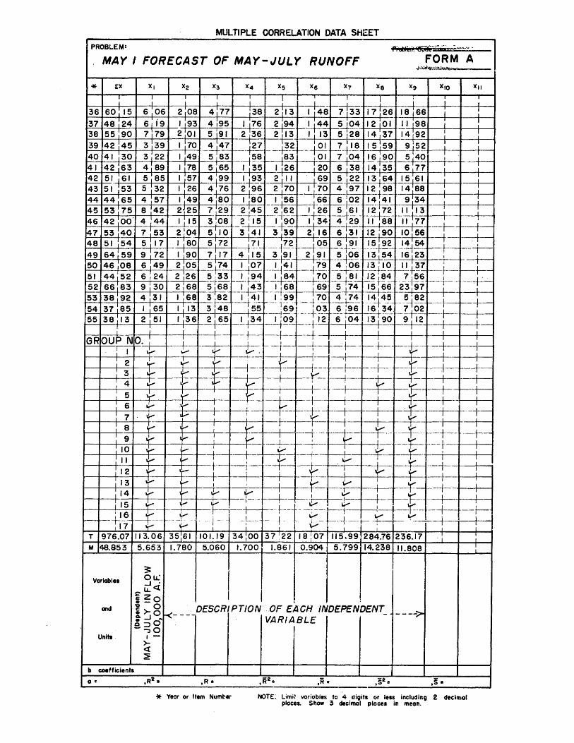
MULTIPLE CORRELATION DATA SHEET PROBLEM:

MAY I FORECAST OF MAY-JULY RUNOFF FORM A

Variables

ond

Units

b coefficients

0 c

3

i~~ I I I I I>- 8 ~--~-_DESCRIPTION' OF EA'CH INDEPENDENT_ c!; 3 0 1' VARIABLE J -'--:;,0 I->­

<{

~

,R • ,'R" ,sa=

---->

,s • * Year or Item Numt-er NOTE: Lirriit variables to 4 digits or leas including 2 decimal

places. Show 3 decimal places in mean.

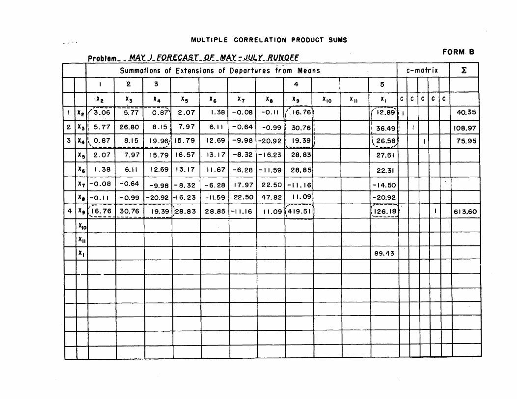
MULTIPLE CORRELATION PRODUCT SUMS

Problem __ M.4'r _l_fO_REC/4_S..T __ Qf: _M~_y_ ~-J_U.LY_.RIJN.QEE FORM. B

Summations of Extensions of Departures from Means c-matrix I '2 3 4 5

)(2 )(3 x4 )(5 )(6 )(7 x, x, x,o Xu X1 I C I C I C I C I C

5~771--o ~a7'J 2. o1 ,

I. 38 I -0.08 I -0.11 1/. 16 .. 76ll I I

I I X21('3:0 ... 6 I

r'i 2.89'~ , 1 II

40.35

2 1 x31! 5. 77 26.80 8.15 I 7.97 6.11 1 -0.641 -0.99 [ 30.761: I I' I 36.49 I l I :_t:_ I

108.97

e.~: j_ ~:_._9~)1 15.79 3 I X4l~ 0.87 ' ...

12.691-9.981-20.921: 19.39v "------- -

\ 26.581 I I I , __ ___ .,, 75.95

X5l 2.07 . 7.97 I 15.791 16.57 13. I 7 1 -8.32 1-16.23 I 28.83 27.51

X61 I .38 6.11 12.69113.17 I 11.671-6.281-11.591 28.85 22.31

X71-0.08I-0.641 -9.981-8.321-6.281 17.971 22.501-11.16 -14.50

Xel-0. II I -0.99 l-2.0.92 l-16. 23 I -11.59 I 22.50 I 4 7. 82 I II. 09 -20.92

4 I x, (_i~~ :~1-~~:_7_6_1_~?.:~~])28~83T 28~85,-1-1.16 r~ 1.09 r419.51ll I

I~ 126,18 '-----_....J_

613.60

X1o

Xu

)(I 89~43

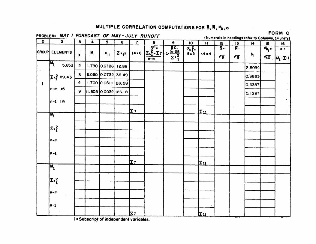
MULTIPLE CORRELATION COMPUTATIONS FOR §, ~. crb,a

RUNOFF FORM C

0 2 3 4 5 6 7 8 9 ~- ---- ----- ·-- -----····- .. -·-·· ~ .... _ ................. ,. ..... .,.

10 1.1 12 13 14 15 16 s2= R2= crbf= 5= R·= Obi= a=

Ix~~I7 1 (n-1)8 ~ROUP ELEMENTS i M· . c ii Ix1xi 14x6 '-:::y 8x5 14x4 Vi vg bi YtO * . I

M1-Iu n-m Ixt IM1 5.653 2 1:.780 0.6786 12.89 2.5084

~xf 89.43 3 5.060 0.0732 36.49 0.3883

I 4 1.700 0.061 t 26.58 0.9387 n-m 15

9 11.808 0.0032 126.18 0.1287

n-1 19

I7 Itt Mt

Ix2 1

n-m

n-1

I1 Itt M1

Ix~

n-m

n-1

I1 I11 i = Subscript of independent variables.

- . ·-· ·- ~-

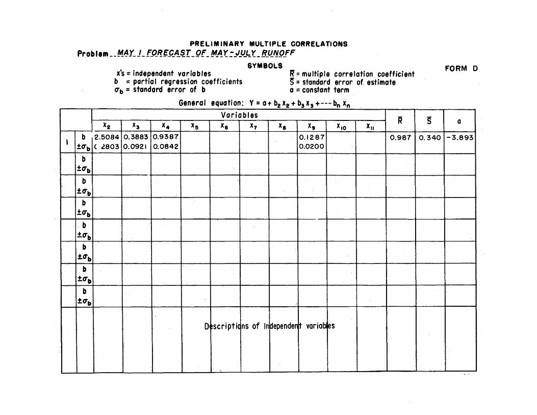
I

PRELIMINARY MULTIPLE CORRELATIONS Prob I em __ M~Y~ J _· f_QI!.~.PA$_ r _ Qf _ !!f_f! '( ~ _J_u_L:_ r. _ B_u_ ~gfF

SYMBOLS x's =independent variables R" =multiple correlation coefficient

b = partial regression coefficients ~: standard error of. estimate ub = standard error of b a = constant term

General equation: Y = a+ b2 x2 + b3 X3 +--- bn Xn

Variables R x2 X! x ... Xs x6 x7 X a x, x,o x ..

b 2.5084 0.3883 0.9387 0.1287 0.987 ±O"b ( l803 0.0921 0.0842 0.0200

b ±crb

b ±crb

b ±O"b

.. b ±.0" b

b .:I:.CTb

b :t.crb

b ±crb

D ~scriptic ns of In dependen t variab ~s

\

FORM D

5 a

0.340 -3.893

~ I

- .

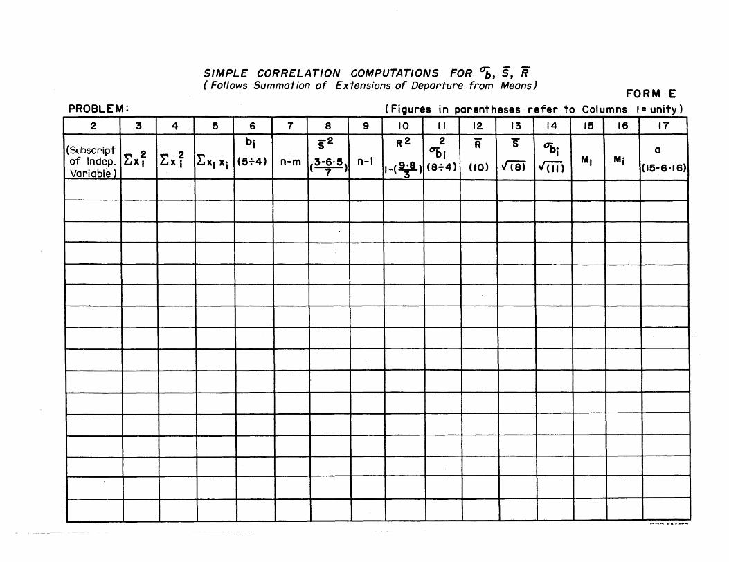
PROBLEM:

2 3 4

{Subscript Ex~ !:x ~ of lndep.

variable}

SIMPLE CORRELATION COMPUTATIONS FOR ~~ S, R (Follows Summation of Extensions of Departure from Means)

FORM E (Figures in parentheses refer to Columns I= unity}

5 6 7 8 9 10 II 12 13 14 15 16 17 b· -2 R2 2 R s ot,i I s

ot,i a Lx1 xi (5+4) 3-6·5 n-1 Ml Mi n-m 1-<Y.> (8+4) ( 10) "18) "fiil (15-6 ·16) ( 7 )

--- -- .. ·--