Multiple Comparison Procedures Comfort Ratings of 13 Fabric Types A.V. Cardello, C. Winterhalter, and H.G. Schultz (2003). "Predicting the Handle and Comfort

Multiple Comparison Procedures

Comfort Ratings of 13 Fabric Types

A.V. Cardello, C. Winterhalter, and H.G. Schultz (2003). "Predicting the Handle and Comfort of Military Clothing Fabrics from Sensory and Instrumental Data: Development and Application of New Psychophysical Methods," Textile Research Journal, Vol. 73, pp. 221-237.

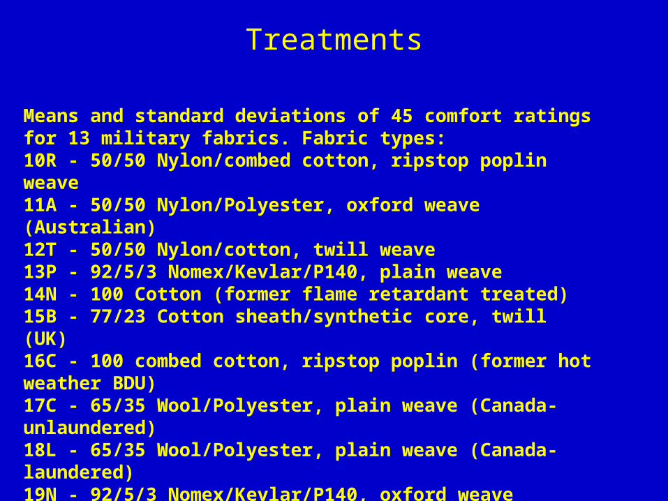
Treatments

Means and standard deviations of 45 comfort ratings for 13 military fabrics. Fabric types: 10R - 50/50 Nylon/combed cotton, ripstop poplin weave 11A - 50/50 Nylon/Polyester, oxford weave (Australian) 12T - 50/50 Nylon/cotton, twill weave 13P - 92/5/3 Nomex/Kevlar/P140, plain weave 14N - 100 Cotton (former flame retardant treated) 15B - 77/23 Cotton sheath/synthetic core, twill (UK) 16C - 100 combed cotton, ripstop poplin (former hot weather BDU) 17C - 65/35 Wool/Polyester, plain weave (Canada-unlaundered) 18L - 65/35 Wool/Polyester, plain weave (Canada-laundered) 19N - 92/5/3 Nomex/Kevlar/P140, oxford weave 20J - Carded cotton sheath/nylon core, plain weave (Canada) 124 - 100 Pima cotton ripstop poplin (experimental) 176 - 50/50 Nylon carded cotton ripstop poplin weave

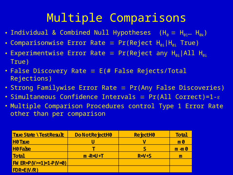
Multiple Comparisons• Individual & Combined Null Hypotheses (H0 H01… H0k)

• Comparisonwise Error Rate Pr(Reject H0i|H0i True)

• Experimentwise Error Rate Pr(Reject any H0i|All H0i True)

• False Discovery Rate E(# False Rejects/Total Rejections)• Strong Familywise Error Rate Pr(Any False Discoveries)• Simultaneous Confidence Intervals Pr(All Correct)=1-• Multiple Comparison Procedures control Type 1 Error Rate

other than per comparisonTrue State \ Test Result Do Not Reject H0 Reject H0 TotalH0 True U V m0H0 False T S m-m0Total m-R=U+T R=V+S mFWER=P(V>=1)=1-P(V=0)FDR=E(V/R)

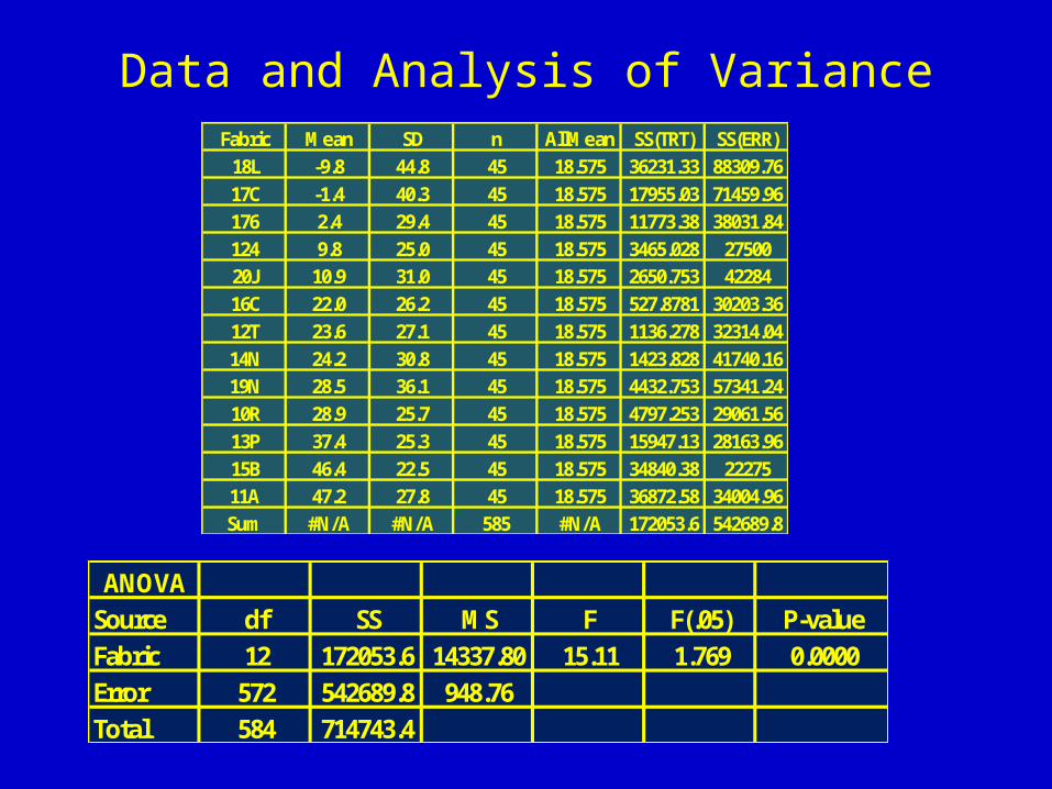
Data and Analysis of VarianceFabric Mean SD n AllMean SS(TRT) SS(ERR)

18L -9.8 44.8 45 18.575 36231.33 88309.7617C -1.4 40.3 45 18.575 17955.03 71459.96176 2.4 29.4 45 18.575 11773.38 38031.84124 9.8 25.0 45 18.575 3465.028 2750020J 10.9 31.0 45 18.575 2650.753 4228416C 22.0 26.2 45 18.575 527.8781 30203.3612T 23.6 27.1 45 18.575 1136.278 32314.0414N 24.2 30.8 45 18.575 1423.828 41740.1619N 28.5 36.1 45 18.575 4432.753 57341.2410R 28.9 25.7 45 18.575 4797.253 29061.5613P 37.4 25.3 45 18.575 15947.13 28163.9615B 46.4 22.5 45 18.575 34840.38 2227511A 47.2 27.8 45 18.575 36872.58 34004.96Sum #N/A #N/A 585 #N/A 172053.6 542689.8

ANOVASource df SS MS F F(.05) P-valueFabric 12 172053.6 14337.80 15.11 1.769 0.0000Error 572 542689.8 948.76Total 584 714743.4

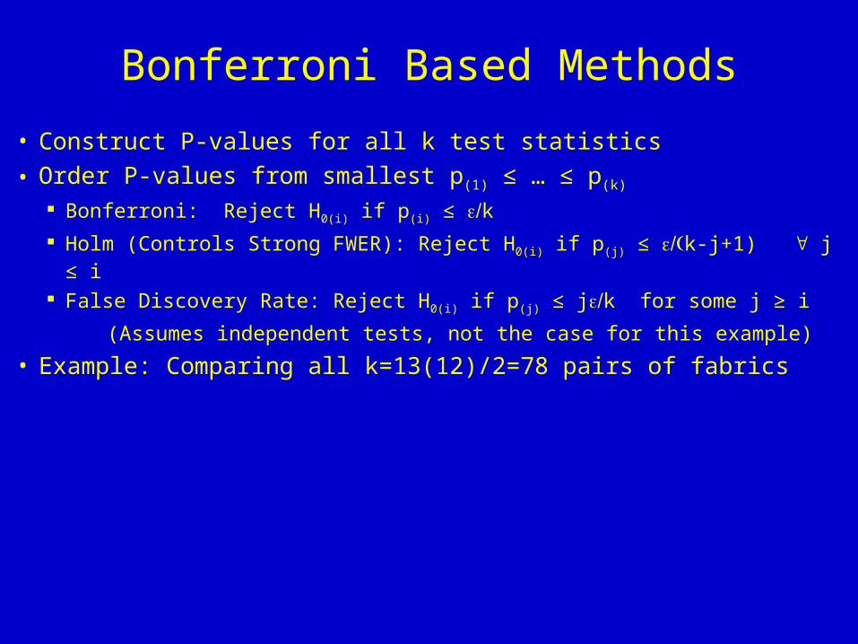
Bonferroni Based Methods

• Construct P-values for all k test statistics• Order P-values from smallest p(1) ≤ … ≤ p(k)

Bonferroni: Reject H0(i) if p(i) ≤ k Holm (Controls Strong FWER): Reject H0(i) if p(j) ≤ k-j+1) j ≤ i

False Discovery Rate: Reject H0(i) if p(j) ≤ jk for some j ≥ i

(Assumes independent tests, not the case for this example)

• Example: Comparing all k=13(12)/2=78 pairs of fabrics

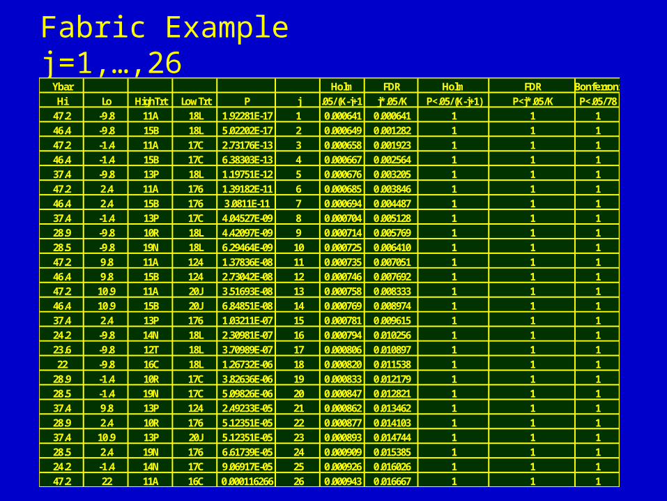
Fabric Example j=1,…,26Ybar Holm FDR Holm FDR Bonferroni

Hi Lo HighTrt LowTrt P j .05/(K-j+1) j*.05/K P<.05/(K-j+1) P<j*.05/K P<.05/7847.2 -9.8 11A 18L 1.92281E-17 1 0.000641 0.000641 1 1 146.4 -9.8 15B 18L 5.02202E-17 2 0.000649 0.001282 1 1 147.2 -1.4 11A 17C 2.73176E-13 3 0.000658 0.001923 1 1 146.4 -1.4 15B 17C 6.38303E-13 4 0.000667 0.002564 1 1 137.4 -9.8 13P 18L 1.19751E-12 5 0.000676 0.003205 1 1 147.2 2.4 11A 176 1.39182E-11 6 0.000685 0.003846 1 1 146.4 2.4 15B 176 3.0811E-11 7 0.000694 0.004487 1 1 137.4 -1.4 13P 17C 4.04527E-09 8 0.000704 0.005128 1 1 128.9 -9.8 10R 18L 4.42097E-09 9 0.000714 0.005769 1 1 128.5 -9.8 19N 18L 6.29464E-09 10 0.000725 0.006410 1 1 147.2 9.8 11A 124 1.37836E-08 11 0.000735 0.007051 1 1 146.4 9.8 15B 124 2.73042E-08 12 0.000746 0.007692 1 1 147.2 10.9 11A 20J 3.51693E-08 13 0.000758 0.008333 1 1 146.4 10.9 15B 20J 6.84851E-08 14 0.000769 0.008974 1 1 137.4 2.4 13P 176 1.03211E-07 15 0.000781 0.009615 1 1 124.2 -9.8 14N 18L 2.30981E-07 16 0.000794 0.010256 1 1 123.6 -9.8 12T 18L 3.70989E-07 17 0.000806 0.010897 1 1 122 -9.8 16C 18L 1.26732E-06 18 0.000820 0.011538 1 1 1

28.9 -1.4 10R 17C 3.82636E-06 19 0.000833 0.012179 1 1 128.5 -1.4 19N 17C 5.09826E-06 20 0.000847 0.012821 1 1 137.4 9.8 13P 124 2.49233E-05 21 0.000862 0.013462 1 1 128.9 2.4 10R 176 5.12351E-05 22 0.000877 0.014103 1 1 137.4 10.9 13P 20J 5.12351E-05 23 0.000893 0.014744 1 1 128.5 2.4 19N 176 6.61739E-05 24 0.000909 0.015385 1 1 124.2 -1.4 14N 17C 9.06917E-05 25 0.000926 0.016026 1 1 147.2 22 11A 16C 0.000116266 26 0.000943 0.016667 1 1 1

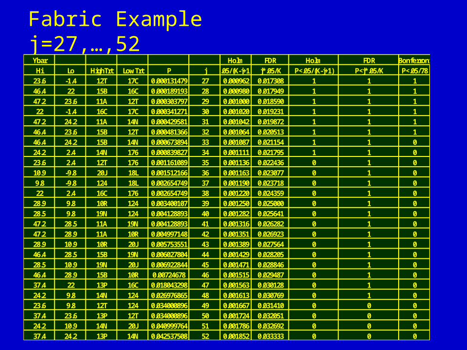
Fabric Example j=27,…,52Ybar Holm FDR Holm FDR Bonferroni

Hi Lo HighTrt LowTrt P j .05/(K-j+1) j*.05/K P<.05/(K-j+1) P<j*.05/K P<.05/7823.6 -1.4 12T 17C 0.000131479 27 0.000962 0.017308 1 1 146.4 22 15B 16C 0.000189193 28 0.000980 0.017949 1 1 147.2 23.6 11A 12T 0.000303797 29 0.001000 0.018590 1 1 122 -1.4 16C 17C 0.000341271 30 0.001020 0.019231 1 1 1

47.2 24.2 11A 14N 0.000429581 31 0.001042 0.019872 1 1 146.4 23.6 15B 12T 0.000481366 32 0.001064 0.020513 1 1 146.4 24.2 15B 14N 0.000673894 33 0.001087 0.021154 1 1 024.2 2.4 14N 176 0.000839827 34 0.001111 0.021795 1 1 023.6 2.4 12T 176 0.001161089 35 0.001136 0.022436 0 1 010.9 -9.8 20J 18L 0.001512166 36 0.001163 0.023077 0 1 09.8 -9.8 124 18L 0.002654749 37 0.001190 0.023718 0 1 022 2.4 16C 176 0.002654749 38 0.001220 0.024359 0 1 0

28.9 9.8 10R 124 0.003400107 39 0.001250 0.025000 0 1 028.5 9.8 19N 124 0.004128893 40 0.001282 0.025641 0 1 047.2 28.5 11A 19N 0.004128893 41 0.001316 0.026282 0 1 047.2 28.9 11A 10R 0.004997148 42 0.001351 0.026923 0 1 028.9 10.9 10R 20J 0.005753551 43 0.001389 0.027564 0 1 046.4 28.5 15B 19N 0.006027804 44 0.001429 0.028205 0 1 028.5 10.9 19N 20J 0.006922844 45 0.001471 0.028846 0 1 046.4 28.9 15B 10R 0.00724678 46 0.001515 0.029487 0 1 037.4 22 13P 16C 0.018043298 47 0.001563 0.030128 0 1 024.2 9.8 14N 124 0.026976865 48 0.001613 0.030769 0 1 023.6 9.8 12T 124 0.034000896 49 0.001667 0.031410 0 0 037.4 23.6 13P 12T 0.034000896 50 0.001724 0.032051 0 0 024.2 10.9 14N 20J 0.040999764 51 0.001786 0.032692 0 0 037.4 24.2 13P 14N 0.042537508 52 0.001852 0.033333 0 0 0

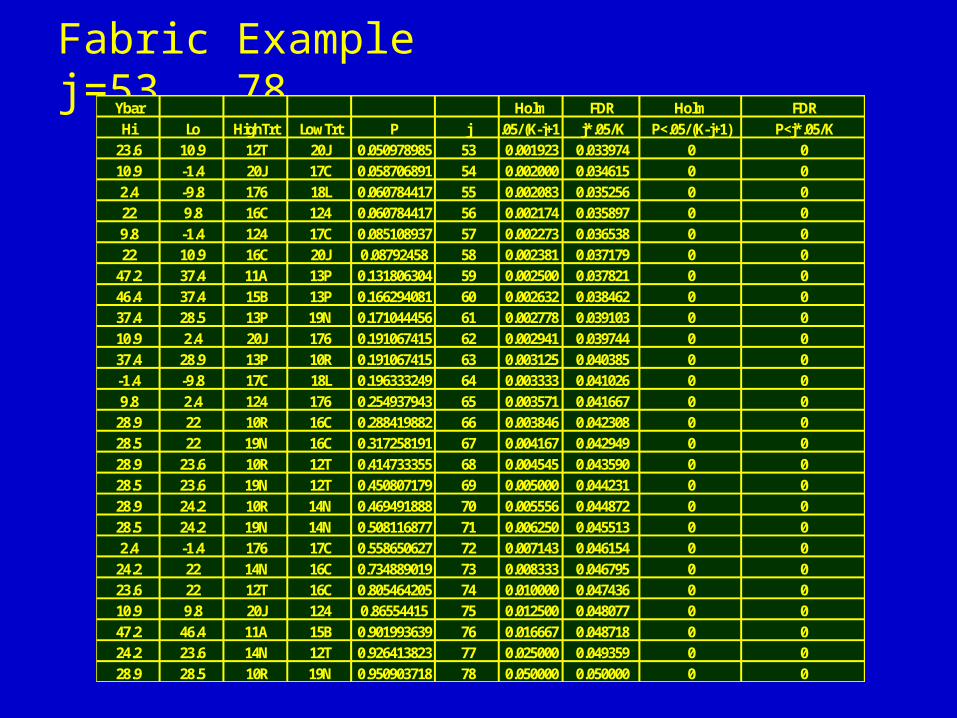
Fabric Example j=53,…,78Ybar Holm FDR Holm FDR

Hi Lo HighTrt LowTrt P j .05/(K-j+1) j*.05/K P<.05/(K-j+1) P<j*.05/K23.6 10.9 12T 20J 0.050978985 53 0.001923 0.033974 0 010.9 -1.4 20J 17C 0.058706891 54 0.002000 0.034615 0 02.4 -9.8 176 18L 0.060784417 55 0.002083 0.035256 0 022 9.8 16C 124 0.060784417 56 0.002174 0.035897 0 09.8 -1.4 124 17C 0.085108937 57 0.002273 0.036538 0 022 10.9 16C 20J 0.08792458 58 0.002381 0.037179 0 0

47.2 37.4 11A 13P 0.131806304 59 0.002500 0.037821 0 046.4 37.4 15B 13P 0.166294081 60 0.002632 0.038462 0 037.4 28.5 13P 19N 0.171044456 61 0.002778 0.039103 0 010.9 2.4 20J 176 0.191067415 62 0.002941 0.039744 0 037.4 28.9 13P 10R 0.191067415 63 0.003125 0.040385 0 0-1.4 -9.8 17C 18L 0.196333249 64 0.003333 0.041026 0 09.8 2.4 124 176 0.254937943 65 0.003571 0.041667 0 0

28.9 22 10R 16C 0.288419882 66 0.003846 0.042308 0 028.5 22 19N 16C 0.317258191 67 0.004167 0.042949 0 028.9 23.6 10R 12T 0.414733355 68 0.004545 0.043590 0 028.5 23.6 19N 12T 0.450807179 69 0.005000 0.044231 0 028.9 24.2 10R 14N 0.469491888 70 0.005556 0.044872 0 028.5 24.2 19N 14N 0.508116877 71 0.006250 0.045513 0 02.4 -1.4 176 17C 0.558650627 72 0.007143 0.046154 0 0

24.2 22 14N 16C 0.734889019 73 0.008333 0.046795 0 023.6 22 12T 16C 0.805464205 74 0.010000 0.047436 0 010.9 9.8 20J 124 0.86554415 75 0.012500 0.048077 0 047.2 46.4 11A 15B 0.901993639 76 0.016667 0.048718 0 024.2 23.6 14N 12T 0.926413823 77 0.025000 0.049359 0 028.9 28.5 10R 19N 0.950903718 78 0.050000 0.050000 0 0

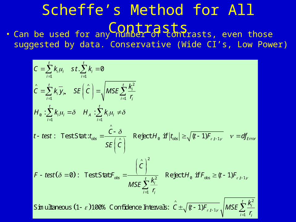
Scheffe’s Method for All Contrasts• Can be used for any number of contrasts, even those

suggested by data. Conservative (Wide CI’s, Low Power)

1 1

2^ ^

1 1

01 1

^

0 , 1,^

2^

. . 0

: :

: Test Stat : Reject if ( 1)

0 : Test Stat:

t t

i i ii i

t ti

i ii i i

t t

i i A i ii i

obs obs t Error

obs

C k s t k

kC k y SE C MSE

r

H k H k

Ct test t H t t F df

SE C

CF test F

M

0 obs , 1,2

1

2^

, 1,1

Reject if ( 1)

Simultaneous 1 100% Confidence Intervals: ( 1)

tti

i i

ti

ti i

H F t Fk

SEr

kC t F MSE

r

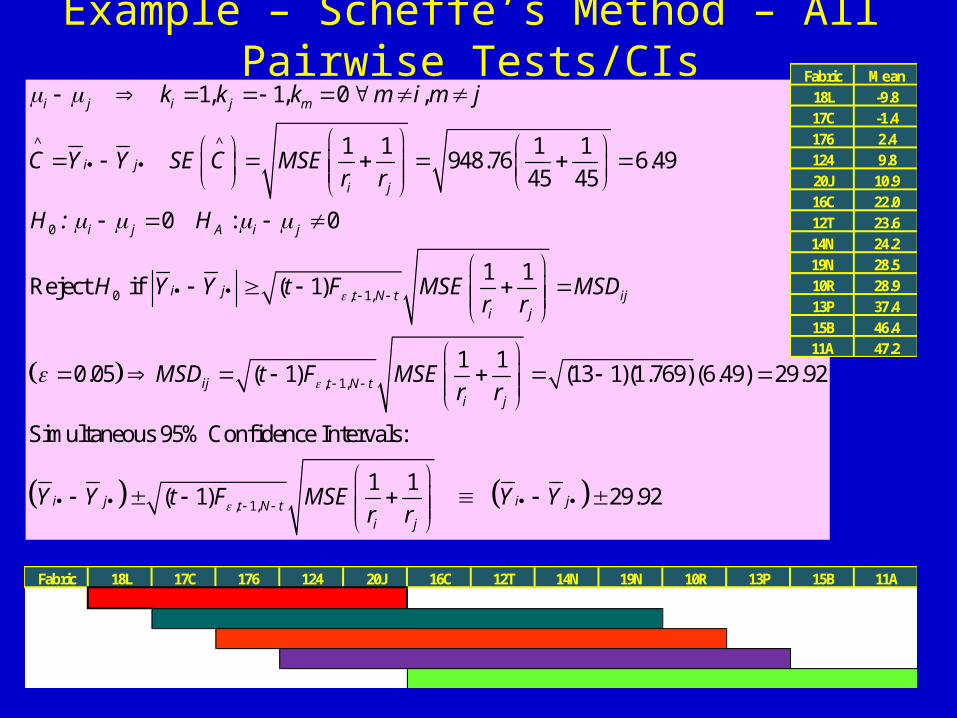
Example – Scheffe’s Method – All Pairwise Tests/CIs

^ ^

0

0 , 1,

, 1

1, 1, 0 ,

1 1 1 1948.76 6.49

45 45

0 : 0

1 1Reject if ( 1)

0.05 ( 1)

i j i j m

i j

i j

i j A i j

i j t N t iji j

ij t

k k k m i m j

C Y Y SE C MSEr r

H : H

H Y Y t F MSE MSDr r

MSD t F

,

, 1,

1 1(13 1)(1.769)(6.49) 29.92

Simultaneous 95% Confidence Intervals:

1 1( 1) 29.92

N ti j

i j i jt N ti j

MSEr r

Y Y t F MSE Y Yr r

Fabric 18L 17C 176 124 20J 16C 12T 14N 19N 10R 13P 15B 11A

Fabric Mean18L -9.817C -1.4176 2.4124 9.820J 10.916C 22.012T 23.614N 24.219N 28.510R 28.913P 37.415B 46.411A 47.2

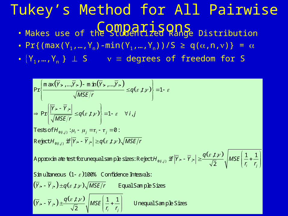
Tukey’s Method for All Pairwise Comparisons• Makes use of the Studentized Range Distribution• Pr{(max(Y1,…,Yn)-min(Y1,…,Yn))/S ≥ q(,n,)} =

• Y1,…,Yn } S degrees of freedom for S

1 1

0( , )

0( , )

max ,..., min ,...,Pr , , 1

Pr , , 1 ,

Tests of : 0 :

Reject if , ,

Approximate test for unequal sample si

t t

i j

i j i j i j

i ji j

Y Y Y Yq t

MSE r

Y Yq t i j

MSE r

H

H Y Y q t MSE r

0( , )

, , 1 1zes: Reject if

2

Simultaneous 1 100% Confidence Intervals:

, , Equal Sample Sizes

, , 1 1 Unequal Sample

2

i ji ji j

i j

i j

i j

q tH Y Y MSE

r r

Y Y q t MSE r

q tY Y MSE

r r

Sizes

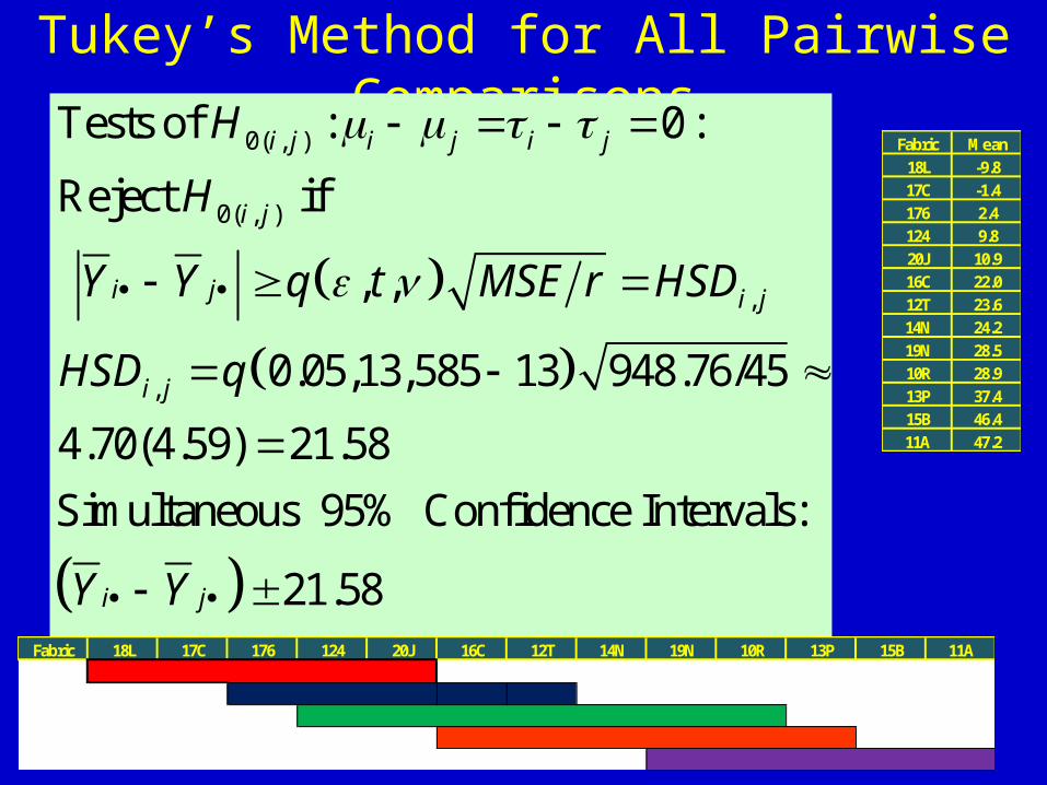
Tukey’s Method for All Pairwise Comparisons

0( , )

0( , )

,

,

Tests of : 0 :

Reject if

, ,

0.05,13,585 13 948.76/45

4.70(4.59) 21.58

Simultaneous 95% Confidence Intervals:

21.58

i j i j i j

i j

i j i j

i j

i j

H

H

Y Y q t MSE r HSD

HSD q

Y Y



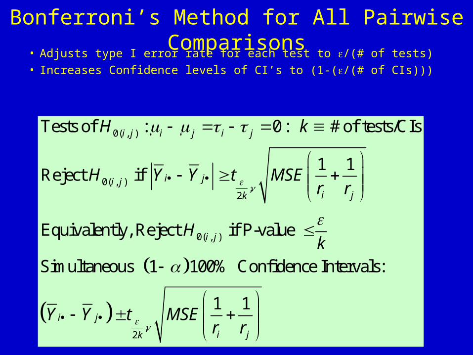
Bonferroni’s Method for All Pairwise Comparisons• Adjusts type I error rate for each test to /(# of tests)• Increases Confidence levels of CI’s to (1-(/(# of CIs)))

0( , )

0( , ),

2

0( , )

2

Tests of : 0 : # of tests/CIs

1 1Reject if

Equivalently, Reject if P-value


i j i j i j

i ji ji jk

i j

i j

k

H k

H Y Y t MSEr r

Hk

Y Y t

,

1 1

i j

MSEr r

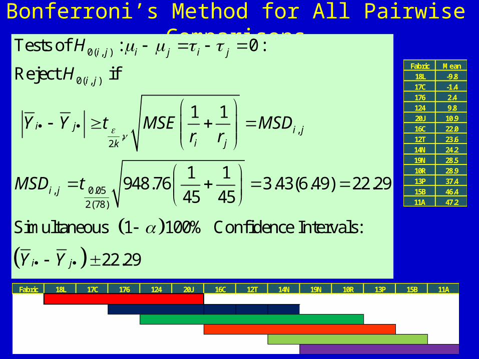
Bonferroni’s Method for All Pairwise Comparisons

0( , )

0( , )

,,

2

, 0.05

2(78)

Tests of : 0 :

Reject if

1 1

1 1948.76 3.43(6.49) 22.29

45 45


22.29

i j i j i j

i j

i j i ji jk

i j

i j

H

H

Y Y t MSE MSDr r

MSD t

Y Y



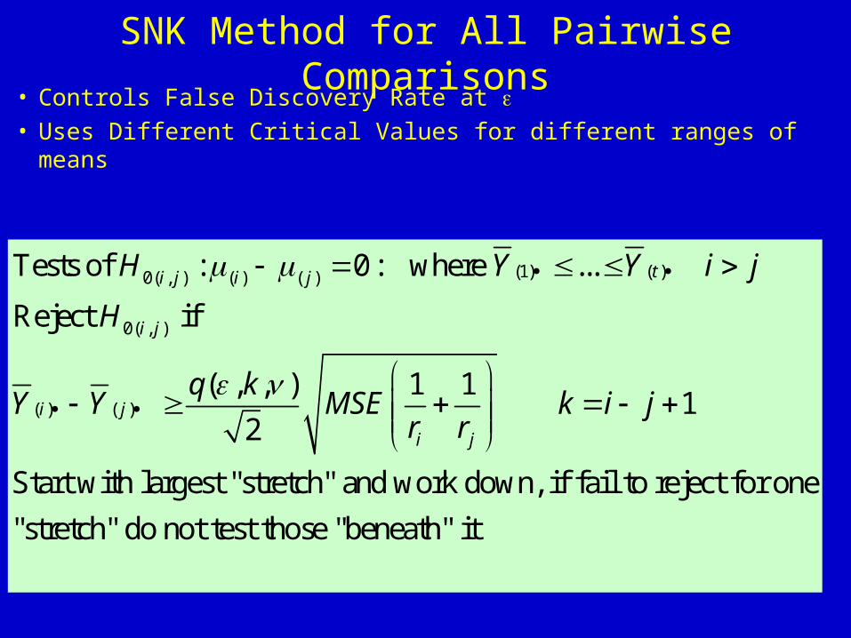
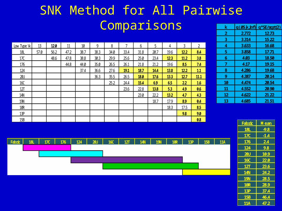
SNK Method for All Pairwise Comparisons• Controls False Discovery Rate at • Uses Different Critical Values for different ranges of means

(1) ( )0( , ) ( ) ( )

0( , )

( ) ( )

Tests of : 0 : where ...

Reject if

( , , ) 1 1 1

2

Start with largest "stretch" and work down, if fail to reject for one

"stretch" d

ti j i j

i j

i j

i j

H Y Y i j

H

q kY Y MSE k i j

r r

o not test those "beneath" it

SNK Method for All Pairwise Comparisons

0( , ) ( ) ( )

(1) ( )

0( , )

( ) ( )

Tests of : 0 :

where ...

Reject if

( , , ) 1 1 1

2

( , , ) 1 1 ( , , )948.76 (6.49)

45 452 2

i j i j

t

i j

i j ki j

k

H

Y Y i j

H

q kY Y MSE MSD k i j

r r

q k q kMSD


k q(.05,k,inf) q*SE/sqrt(2)2 2.772 12.733 3.314 15.224 3.633 16.685 3.858 17.716 4.03 18.507 4.17 19.158 4.286 19.689 4.387 20.1410 4.474 20.5411 4.552 20.9012 4.622 21.2213 4.685 21.51


SNK Method for All Pairwise Comparisons


k q(.05,k,inf) q*SE/sqrt(2)2 2.772 12.733 3.314 15.224 3.633 16.685 3.858 17.716 4.03 18.507 4.17 19.158 4.286 19.689 4.387 20.1410 4.474 20.5411 4.552 20.9012 4.622 21.2213 4.685 21.51

Low Type \k 13 12.0 11 10 9 8 7 6 5 4 3 218L 57.0 56.2 47.2 38.7 38.3 34.0 33.4 31.8 20.7 19.6 12.2 8.417C 48.6 47.8 38.8 30.3 29.9 25.6 25.0 23.4 12.3 11.2 3.8176 44.8 44.0 35.0 26.5 26.1 21.8 21.2 19.6 8.5 7.4124 37.4 36.6 27.6 19.1 18.7 14.4 13.8 12.2 1.120J 36.3 35.5 26.5 18.0 17.6 13.3 12.7 11.116C 25.2 24.4 15.4 6.9 6.5 2.2 1.612T 23.6 22.8 13.8 5.3 4.9 0.614N 23.0 22.2 13.2 4.7 4.319N 18.7 17.9 8.9 0.410R 18.3 17.5 8.513P 9.8 9.015B 0.8


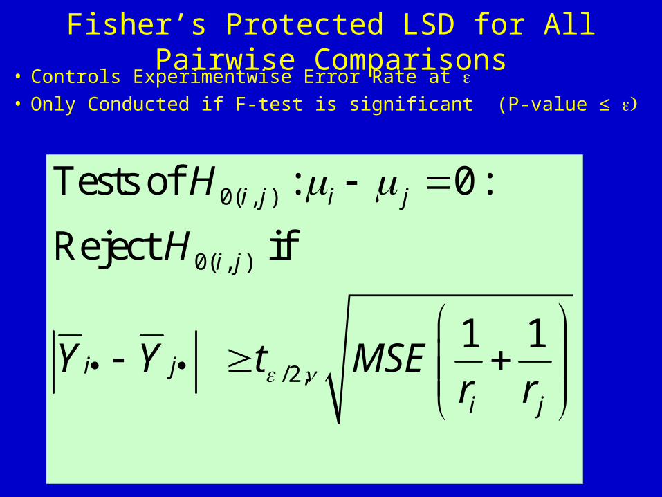
Fisher’s Protected LSD for All Pairwise Comparisons• Controls Experimentwise Error Rate at • Only Conducted if F-test is significant (P-value ≤

0( , )

0( , )

/2,

Tests of : 0 :

Reject if

1 1

i j i j

i j

i j

i j

H

H

Y Y t MSEr r

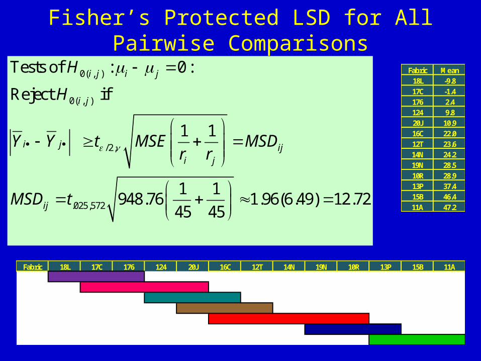
Fisher’s Protected LSD for All Pairwise Comparisons

0( , )

0( , )

/2,

.025,572

Tests of : 0 :

Reject if

1 1

1 1948.76 1.96(6.49) 12.72

45 45

i j i j

i j

i j iji j

ij

H

H

Y Y t MSE MSDr r

MSD t



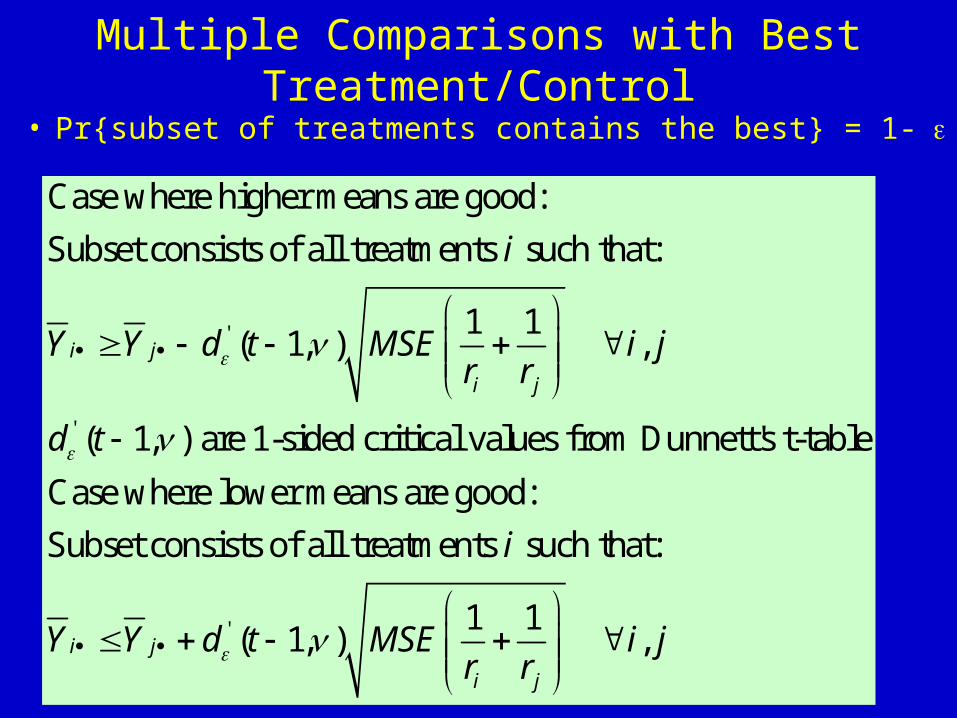
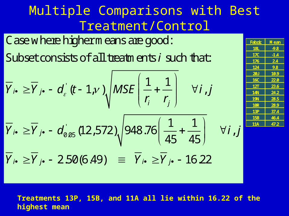
Multiple Comparisons with Best Treatment/Control

• Pr{subset of treatments contains the best} = 1-

'

'

Case where higher means are good:

Subset consists of all treatments such that:

1 1( 1, ) ,

( 1, ) are 1-sided critical values from Dunnett's t-table

Case where lower mea

i j

i j

i

Y Y d t MSE i jr r

d t

'

ns are good:


1 1( 1, ) ,i j

i j

i

Y Y d t MSE i jr r

Multiple Comparisons with Best Treatment/Control

'

'0.05

Case where higher means are good:


1 1( 1, ) ,

1 1(12,572) 948.76 ,

45 45

2.50(6.49) 16.22

i j

i j

i j

i j i j

i

Y Y d t MSE i jr r

Y Y d i j

Y Y Y Y


Treatments 13P, 15B, and 11A all lie within 16.22 of the highest mean

Documents

Multiple Comparison Procedures Comfort Ratings of 13 Fabric Types A.V. Cardello, C. Winterhalter, and H.G. Schultz (2003). "Predicting the Handle and Comfort