MULTIPLE-CHOICE QUESTIONS (MCQ) EXAMINATION … · MULTIPLE-CHOICE QUESTIONS (MCQ) EXAMINATION DURATION: 100 MINUTES Annotations to the assignments and the solution sheet This is

University of Duisburg-Essen

Prof. Dr.-Ing. Axel Hunger Institute of Computer Engineering

WS 2017 / 2018

DEMO-EXAMINATION Test and Reliability of Digital Systems Page: 1 of 19

Name Matriculation number Type

MULTIPLE-CHOICE QUESTIONS (MCQ) EXAMINATION

DURATION: 100 MINUTES

Annotations to the assignments and the solution sheet This is a multiple choice examination, that means:

Solution approaches are not assessed.

For each subtask there is only one correct solution.

For each subtask you are allowed to mark one box only. If two or more boxes for a subtask are marked, no points will be given for this subtask.

Note the following points

In addition to the assignment sheets there is a solution sheet.

Mark the appropriate box(es) on the solution sheet! Any answer on the ASSIGNMENT SHEETS will NOT be considered.

It is not possible to correct markings in the solution sheet. In case of errors request a new solution sheet. Any earlier solution sheet is substituted only as immediate exchange old against new. The previous erroneous or invalid sheet will be destroyed by the invigilating staff. In case of submission of multiple sheets neither will be evaluated.

Any substitution of solution sheets is only possible up to 5 minutes before the official end of the examination time.

Only use the sheets enclosed in the envelope or otherwise provided by the supervisors. Don't use any other paper. If you need more paper ask the supervisors.

Return everything, i.e. assignment sheets, solution sheet and any additional sheets - used and un-used. Only exams that are returned completely will be assessed.

FILL-IN YOUR NAME AND MATRICULATION NUMBER ON THE ASSIGNMENT SHEET AND THE SOLUTION SHEET!



WS 2017 / 2018



(6 Points)

1.1 Welche der folgenden Aussagen ist wahr?

A: Die Formel für die Ausfallwahrscheinlichkeit lautet F(t)=−𝑑

𝑑𝑡𝑅(𝑡)

B: Bei der Reserve ist ein Teil betriebsführend, während ein oder mehrere Teilsystem(e) vorgehalten werden um im Falle eines Ausfalles zu übernehmen.

C: Der D-Algorithmus benötigt keine Kenntnisse über den Aufbau des Schaltkreises

D: Die genäherte Funktionswerte der Verteilungsfunktion an der Stelle 2σ→95,5% lautet F(x=μ+2·σ)=0,841

E: None of these.

1.2 Welche der folgenden Aussagen ist wahr?

F: Bei der kalten Reserve laufen die Hauptkomponenten und die Reserveeinheit parallel und unabhängig nebeneinander.

G:

Folgendes Bild beschreibt qualitative den Verlauf der Ausfallrate bei negativer Exponentialverteilung:

H: Diagnostisches Testen findet immer die geringste Anzahl an Testmustern

I: Die Bool‘sche Differenz kann verwendet werden um interne Fehler unveränderter Schaltungen aufzudecken.

J: None of these.

λ(x)

x



WS 2017 / 2018



(16 Punkte)

2.1 Für die Produktionsreihe eines Gerätes wurde eine mittlere Lebensdauer von 100000h ermittelt. Die Lebensdauer ist negativ exponentialverteilt.

Wie groß ist die Wahrscheinlichkeit, dass ein Gerät aus dieser Produktionsreihe 20000 Betriebsstunden überlebt? (Runden sie auf die 3. Nachkommastelle)

A: R(tm) = 0,787 B: R(tm) = 0,802 C: R(tm) = 0,819

D: R(tm) = 0,844 E: R(tm) = 0,901 F: None of these.

2.2 Auf einer 1000 km langen Autobahnstrecke kommt es durchschnittlich 200 mal pro Jahr zu Behinderungen, die eine Verzögerung von mehr als 30 Minuten zur Folge haben.

Mit welcher Wahrscheinlichkeit kommt es auf einem 200 km langen Abschnitt dieser Strecke zu mindestens zwei Behinderungen dieser Art an einem Tag? (Gerundet auf die 4. Nachkommastelle)

G: P(X > 1) = 0,011 H: P(X > 1) = 0,0098 I: P(X > 1) = 0,0075

J: P(X > 1) = 0,0056 K: P(X > 1) = 0,0038 L: None of these.

2.3 Auf einer 1000 km langen Autobahnstrecke kommt es durchschnittlich 200 mal pro Jahr zu Behinderungen, die eine Verzögerung von mehr als 30 Minuten zur Folge haben.

Mit welcher Wahrscheinlichkeit kommt es auf einem 200 km langen Abschnitt dieser Strecke zu genau drei Behinderungen dieser Art an einem Tag, unter der Voraussetzung, dass es an dem Tag bereits mindestens eine Behinderung gab? (Gerundet auf die 6. Nachkommastelle)

M: P(X=3 | X ≥ 1) = 4,894 • 10-3 N: P(X=3 | X ≥ 1) = 3,022 • 10-3

O: P(X=3 | X ≥ 1) = 2,896 • 10-3 P: P(X=3 | X ≥ 1) = 1,896 • 10-3

Q: P(X=3 | X ≥ 1) = 0,449 • 10-3 R: None of these.



WS 2017 / 2018



(9 Points) Gegeben sei ein Gerät, welches aus zwei Komponenten besteht. Nach Ausfall einer Komponente (Ausfallrate λ) wird sie mit der Rate μ wieder instandgesetzt. Der Zustand einer Komponente wird mit ix (instand) und dx (defekt) bezeichnet.

Abb. 3-1 zeigt die Reduzierte Markov-Kette des genannten Systems, Abb. 3-2 die zugehörigen Systemzustände.

i1 ʌ i2 = MZ0

(i1 ʌ d2) ˅ (d1 ʌ i2) = MZ1

d1 ʌ d2 = MZ2

Abb. 3-1: Markov-Kette Abb. 3-2: Systemzustände

3.1 Welche der folgenden Markov-Ketten repräsentiert die nicht-reduzierte Markov-Kette der Systemzustände aus Abb. 3-1

A:

B:

C:

D:

E: None of these.



WS 2017 / 2018



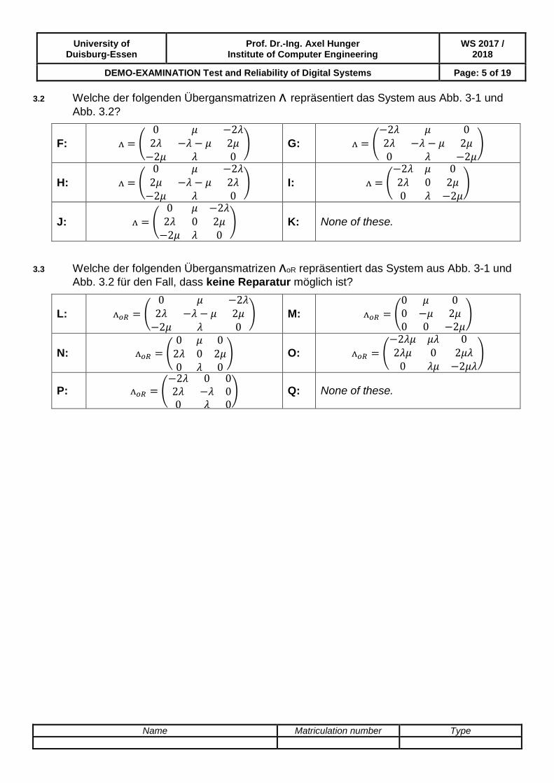
3.2 Welche der folgenden Übergansmatrizen ʌ repräsentiert das System aus Abb. 3-1 und

Abb. 3.2?

F: ʌ = (0 𝜇 −2𝜆

2𝜆 −𝜆 − 𝜇 2𝜇−2𝜇 𝜆 0

) G: ʌ = (−2𝜆 𝜇 02𝜆 −𝜆 − 𝜇 2𝜇0 𝜆 −2𝜇

)

H: ʌ = (0 𝜇 −2𝜆

2𝜇 −𝜆 − 𝜇 2𝜆−2𝜇 𝜆 0

) I: ʌ = (−2𝜆 𝜇 02𝜆 0 2𝜇0 𝜆 −2𝜇

)

J: ʌ = (0 𝜇 −2𝜆

2𝜆 0 2𝜇−2𝜇 𝜆 0

) K: None of these.

3.3 Welche der folgenden Übergansmatrizen ʌoR repräsentiert das System aus Abb. 3-1 und

Abb. 3.2 für den Fall, dass keine Reparatur möglich ist?

L: ʌ𝑜𝑅 = (0 𝜇 −2𝜆

2𝜆 −𝜆 − 𝜇 2𝜇−2𝜇 𝜆 0

) M: ʌ𝑜𝑅 = (0 𝜇 00 −𝜇 2𝜇0 0 −2𝜇

)

N: ʌ𝑜𝑅 = (0 𝜇 0

2𝜆 0 2𝜇0 𝜆 0

) O: ʌ𝑜𝑅 = (−2𝜆𝜇 𝜇𝜆 02𝜆𝜇 0 2𝜇𝜆

0 𝜆𝜇 −2𝜇𝜆)

P: ʌ𝑜𝑅 = (−2𝜆 0 02𝜆 −𝜆 00 𝜆 0

) Q: None of these.



WS 2017 / 2018



(21 Points) Ein Automobilhersteller beginnt mit der Großserienproduktion eines neuen Fahrzeugmodells. Während der Entwicklungsphase wurden 15 Getriebeeinheiten verbaut, deren Laufleistungen bei Ausfall wie folgt dokumentiert wurden:

Getriebe 1 2 3 4 5 6 7 8 9 10 11 12 13 14 15

Lebensdauer (in 1000 km)

340 310 320 320 310 330 300 320 330 300 310 350 280 330 320

Tabelle 4-1: Lebensdauer

4.1 Wählen Sie durch Untersuchung der Stichprobe eine geeignete Lebensdauerverteilung für die produzierten Getriebeeinheiten. Welche der folgenden Ergebnisse repräsentieren den Mittelwert und die Varianz für die Werte aus Tabelle 4-1?

A: �̅̂� = 299000 𝑘𝑚 ; �̂� = 14503 𝑘𝑚 B: �̅̂� = 306000 𝑘𝑚 ; �̂� = 16804 𝑘𝑚

C: �̅̂� = 318000 𝑘𝑚 ; �̂� = 17403 𝑘𝑚 D: �̅̂� = 306000 𝑘𝑚 ; �̂� = 14503 𝑘𝑚

E: �̅̂� = 318000 𝑘𝑚 ; �̂� = 16804 𝑘𝑚 F: �̅̂� = 299000 𝑘𝑚 ; �̂� = 17403 𝑘𝑚

G: None of these.

Die Lebensdauer einer Motorsteuergeräte-Produktionsreihe von wird von der zugehörigen Qualitätsmanagement-Abteilung mit folgenden Parametern beschrieben:

μ = 6000h (Betriebsstunden) σ = 700h (Betriebsstunden)

4.2 Wie groß ist die Wahrscheinlichkeit, dass ein Motorsteuergerät der gleichen Produktionsreihe im Zeitraum von μ-σ bis μ+σ ausfällt? (Gerundet auf die 4. Nachkommastelle)

H: 𝑃(𝜇 − 𝜎 ≤ 𝑥 ≤ 𝜇 + 𝜎) = 0,5774 I: 𝑃(𝜇 − 𝜎 ≤ 𝑥 ≤ 𝜇 + 𝜎) = 0,6826

J: 𝑃(𝜇 − 𝜎 ≤ 𝑥 ≤ 𝜇 + 𝜎) = 0,6122 K: 𝑃(𝜇 − 𝜎 ≤ 𝑥 ≤ 𝜇 + 𝜎) = 0,7264

L: 𝑃(𝜇 − 𝜎 ≤ 𝑥 ≤ 𝜇 + 𝜎) = 0,6673 M: None of these.

4.3 Welche Lebensdauer erreicht ein Motorsteuergerät mit einer Wahrscheinlichkeit von p=0.8?

N: 𝑥 = 206 ℎ O: 𝑥 = 1644 ℎ P: 𝑥 = 2011 ℎ

Q: 𝑥 = 4572 ℎ R: 𝑥 = 5412 ℎ S: None of these.



WS 2017 / 2018



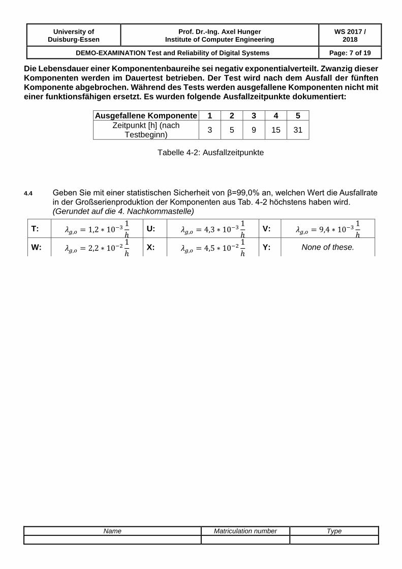
Die Lebensdauer einer Komponentenbaureihe sei negativ exponentialverteilt. Zwanzig dieser Komponenten werden im Dauertest betrieben. Der Test wird nach dem Ausfall der fünften Komponente abgebrochen. Während des Tests werden ausgefallene Komponenten nicht mit einer funktionsfähigen ersetzt. Es wurden folgende Ausfallzeitpunkte dokumentiert:

Ausgefallene Komponente 1 2 3 4 5

Zeitpunkt [h] (nach Testbeginn)

3 5 9 15 31

Tabelle 4-2: Ausfallzeitpunkte

4.4 Geben Sie mit einer statistischen Sicherheit von β=99,0% an, welchen Wert die Ausfallrate in der Großserienproduktion der Komponenten aus Tab. 4-2 höchstens haben wird. (Gerundet auf die 4. Nachkommastelle)

T: 𝜆𝑔,𝑜 = 1,2 ∗ 10−31

ℎ U: 𝜆𝑔,𝑜 = 4,3 ∗ 10−3

1

ℎ V: 𝜆𝑔,𝑜 = 9,4 ∗ 10−3

1

ℎ

W: 𝜆𝑔,𝑜 = 2,2 ∗ 10−21

ℎ X: 𝜆𝑔,𝑜 = 4,5 ∗ 10−2

1

ℎ Y: None of these.



WS 2017 / 2018



(15 Points) Gegeben ist der logische Schaltkreis aus Abb. 5-1, welcher die Funktion Z(x1, x2, x3) realisiert. Der (unvollständige) Fehlertabellenausschnitt aus Abb. 5-2 muss vervollständigt werden um einzelne stuck-at Fehler des Schaltkreises zu analysieren. Die stuck-at Fehler am Ausgang Z werden ignoriert.

Abb. 5-1: Logischer Schaltkreis

Input and fault free output Output Z under condition of a single stuck-at-fault (sa0 / sa1)

Testmuster X1 X2 X3 Z X1|sa0 X1|sa1 X2|sa0 X2|sa1 X3|sa0 X3|sa1 y1|sa0 y1|sa1 y2|sa0 y2|sa1

TP1 0 0 0 1 0 1 0 1 1 0 1 1

TP2 0 0 1 1 0 1 1 1 1 0 1 1

TP3 0 1 0 0 0 0 0 0 1 0 1 0 1

TP4 0 1 1 1 1 1 1 0 1 1 0 1

TP5 1 0 0 0 0 0 0 0 0 0 0 1

TP6 1 0 1 0 0 0 0 0 0 0 1

TP7 1 1 0 0 0 0 0 0 0 1 0 1 0 1

TP8 1 1 1 1 1 1 1 0 1 1 0 1

Abb. 5-2: (Unvollständige) Fehlertabelle

5.1 Wie viele Fehleräquivalenzklassen können von den stuck-at-Fehlern aus der Tabelle in Abb. 5-2 gebildet werden?

A: 5 Fehleräquivalenzklassen B: 6 Fehleräquivalenzklassen

C: 7 Fehleräquivalenzklassen D: 8 Fehleräquivalenzklassen

E: None of these.



WS 2017 / 2018



Gegeben ist der Ausschnitt einer Fehlertabelle für Ausgangswerte bei einzelnen stuck-at Fehlern eines nicht näher spezifizierten Schaltkreises. Die stuck-at Fehler am Ausgang Z werden ignoriert.

Input and fault free output Output Z under condition of a single stuck-at-fault (sa0 / sa1)

Test X1 X2 X3 Z X1|sa0 X1|sa1 X2|sa0 X2|sa1 X3|sa0 X3|sa1 y1|sa0 y1|sa1 y2|sa0 y2|sa1 y3|sa0 y3|sa1

TP1 0 0 0 0 0 1 0 1 0 0 0 0 0 0 0 0

TP2 0 0 1 1 1 0 0 0 1 1 1 1 1 1 1 1

TP3 0 1 0 1 1 1 0 1 0 0 1 1 0 1 0 0

TP4 0 1 1 0 0 0 0 0 0 0 1 0 0 0 0 0

TP5 1 0 0 1 0 1 1 1 1 0 1 1 0 1 0 1

TP6 1 0 1 0 0 0 0 0 0 0 1 0 0 1 0 1

TP7 1 1 0 0 0 1 1 1 0 0 1 0 0 1 0 1

TP8 1 1 1 0 0 0 0 0 0 0 1 0 0 0 0 1

Abb. 5-3: Fehlertabelle mit möglichen Testmustern (TPX =̂ Testmuster X)

5.2 Welches der folgenden Testmustersets erfüllt das Kriterium für das minimale Testmuster-Set für die Tabelle aus Abb. 5-3?

F: TPmin = (TP2,TP3,TP5,TP7) G: TPmin = (TP1,TP4,TP5,TP6)

H: TPmin = (TP3,TP5,TP7) I: TPmin = (TP4,TP5,TP7,TP8)

J: Das minimale Testset enthält alle Testmuster aus Fig. 4-3

K: None of these.

5.3 Welche der folgenden Fehlerauflistungen entspricht dem vollständigen Set aus Fehlern, die über diagnostisches Testen der Tabelle aus Abb. 5-3 gefunden werden können?

L: x2|sa0, y1|sa0, y2|sa1 & y3|sa1 M: x1|sa1, x2|sa0 & y1|sa1

N: x1|sa0 & x2|sa0 O: x1|sa0, x3|sa0, y1|sa1 & y2|sa1

y1|sa1,y2|sa0 & y3|sa0 P: None of these.



WS 2017 / 2018



(9 Points) Gegeben ist der logische Schaltkreis aus Abb. 6.1, welcher die logische Funktion Z(x1,x2,x3) realisiert.


Lösung der Schaltungsgleichung: 𝑍 = 𝑥2 + 𝑥1̅̅̅ ∗ 𝑥3̅̅ ̅ + 𝑥3

6.1 Welche der folgenden logischen Funktionen ist das Resultat der Bool‘schen Differenz 𝛿𝑍

𝑥2

für den Schaltkreis aus Abb. 6-1?

A: 𝑥1 ∗ 𝑥3 B: 𝑥1 + 𝑥3 C: 𝑥1 ∗ 𝑥3

D: 𝑥1 + 𝑥3 E: 𝑥1 + 𝑥3 F: 𝑥1 ∗ �̅�3

G: None of these.

6.2 Welches der folgenden Testmuster qualifiziert sich um den primären Eingang x1 des Schaltkreises aus Abb. 6-1 auf einzelne stuck-at Fehler zu testen?

H: 𝑥1 𝑥2 𝑥3

0 1 0

I: 𝑥1 𝑥2 𝑥3

1 1 0

J: 𝑥1 𝑥2 𝑥3

1 0 1

K: 𝑥1 𝑥2 𝑥3

0 0 0

L: 𝑥1 𝑥2 𝑥3

1 1 1

M: 𝑥1 𝑥2 𝑥3

0 0 1

N: None of these.



WS 2017 / 2018



(14 Points)

Gegeben ist der logische Schaltkreis aus Abb. 7.1, welcher die logische Funktion Z(x1, x2, x3, x4) realisiert.


7.1 Welche der folgenden Tabellen repräsentiert das Ergebnis einer Pfadsensitivierung für einen einzelnen stuck-at-one Fehler am internen Knoten y2 (y2|sa1), des Schaltkreises aus Abb. 7-1?

A: x1 x2 x3 x4 y1 y2 y3 y4 Z

1 1 0 0 1 1 1 1 0

B: x1 x2 x3 x4 y1 y2 y3 y4 Z

1 1 0 0 1 1 0 0 1

C: x1 x2 x3 x4 y1 y2 y3 y4 Z

0 0 1 1 0 0 1 1 0

D: x1 x2 x3 x4 y1 y2 y3 y4 Z

1 1 1 1 0 0 1 1 0

E: x1 x2 x3 x4 y1 y2 y3 y4 Z

0 1 0 1 1 1 0 1 1

F: x1 x2 x3 x4 y1 y2 y3 y4 Z

0 1 0 0 1 0 0 0 1

G: Due to collision, no test pattern can be found H: None of these.



WS 2017 / 2018



Gegeben ist der logische Schaltkreis aus Abb. 7.2, welcher die logische Funktion Z(x1, x2, x3, x4, x5) realisiert.

Fig. 7-2: Logischer Schaltkreis

7.2 Welche der folgenden Tabellen repräsentiert das Ergebnis einer Pfadsensitivierung für einen einzelnen stuck-at-one Fehler am internen Knoten d1 (d1|sa1), des Schaltkreises aus Abb. 7-2?

I: x1 x2 x3 x4 x5 y1 y2 y3 y4 y5 y6 Z

1 1 0 1 1 1 1 0 1 0 0 0

J: x1 x2 x3 x4 x5 y1 y2 y3 y4 y5 y6 Z

1 0 0 0 0 0 1 1 0 1 0 0

K: x1 x2 x3 x4 x5 y1 y2 y3 y4 y5 y6 Z

0 0 0 1 1 1 0 0 1 1 0 1

L: x1 x2 x3 x4 x5 y1 y2 y3 y4 y5 y6 Z

1 0 0 1 1 0 1 0 0 1 0 0

M: x1 x2 x3 x4 x5 y1 y2 y3 y4 y5 y6 Z

0 0 1 1 1 1 0 0 1 1 0 1

N: Due to collision, no test pattern can be found

O: None of these.



WS 2017 / 2018



(10 Points)

Gegeben ist der logische Schaltkreis aus Abb. 7.2, welcher die logische Funktion Z(x1, x2, x3, x4) realisiert.

Fig. 8.1: Logischer Schaltkreis

8.1 Welches der folgenden generellen Test-Sets repräsentiert das komplette Resultat einer D-Algorithmus Analyse von einzelnen stuck-at Fehlern an der Stelle y2, des Schaltkreises aus Abb. 8-1?

A: x1 x2 x3 x4

& x1 x2 x3 x4

& x1 x2 x3 x4

& x1 x2 x3 x4

1 D 0 0 1 �̅� 0 0 0 D 0 0 0 �̅� 0 0

B: x1 x2 x3 x4

& x1 x2 x3 x4

& x1 x2 x3 x4

0 D 1 1 0 �̅� 1 1 1 D 1 1

C: x1 x2 x3 x4

& x1 x2 x3 x4

& x1 x2 x3 x4

& x1 x2 x3 x4

0 D 1 1 0 �̅� 1 1 1 D 1 1 1 �̅� 1 1

D: x1 x2 x3 x4

& x1 x2 x3 x4

0 D 1 1 0 �̅� 1 1

E: x1 x2 x3 x4

& x1 x2 x3 x4

0 D 1 X 0 �̅� 1 X

F: x1 x2 x3 x4

& x1 x2 x3 x4

& x1 x2 x3 x4

X D 0 1 X �̅� 0 1 X �̅� 1 1

G: Due to collision, no test pattern can be found

H: None of these.



WS 2017 / 2018



8.2 Welches der folgenden generellen Test-Sets repräsentiert das komplette Resultat einer D-Algorithmus Analyse von einzelnen stuck-at Fehlern an der Stelle x4, des Schaltkreises aus Abb. 8-1?

I: x1 x2 x3 x4

& x1 x2 x3 x4

& x1 x2 x3 x4

& x1 x2 x3 x4

0 1 0 �̅� 0 1 0 D 1 1 0 �̅� 1 1 0 D

J: x1 x2 x3 x4

& x1 x2 x3 x4

& x1 x2 x3 x4

1 1 1 D 1 1 1 �̅� 1 1 0 �̅�

K: x1 x2 x3 x4

& x1 x2 x3 x4

& x1 x2 x3 x4

& x1 x2 x3 x4

X 1 1 D X 1 1 �̅� X 1 0 D X 1 0 �̅�

L: x1 x2 x3 x4

& x1 x2 x3 x4

X 0 1 �̅� X 0 1 D

M: x1 x2 x3 x4

& x1 x2 x3 x4

0 0 1 �̅� 1 0 1 D

N: x1 x2 x3 x4

& x1 x2 x3 x4

& x1 x2 x3 x4

X 1 X �̅� X 1 X D X 0 X D

O: Due to collision, no test pattern can be found

P: None of these.



WS 2017 / 2018



Tabellen, Hilfsblätter:

𝜒2-Verteilung: 𝜒𝑖,𝛽2 =

𝑖 ↓ \𝛽 → 𝟎, 𝟎𝟎𝟏 𝟎, 𝟎𝟎𝟓 𝟎, 𝟎𝟏𝟎 𝟎, 𝟎𝟓𝟎 𝟎, 𝟏𝟎𝟎 𝟎, 𝟓𝟎𝟎 𝟎, 𝟗𝟎𝟎 𝟎, 𝟗𝟓𝟎 𝟎, 𝟗𝟗𝟎 𝟎, 𝟗𝟗𝟓 𝟎, 𝟗𝟗𝟗

𝛽 =1

√2𝜋∫ 𝑒−

𝑧′2

2𝑑𝑧′

+𝑧𝛽

−𝑧𝛽

𝑧𝛽 =

Standardormalverteilg.:



WS 2017 / 2018



Studentsche t-Verteilung: S̃i,β =

𝒊\𝜷 𝟎. 𝟔𝟎 𝟎. 𝟕𝟓 𝟎. 𝟗𝟎 𝟎. 𝟗𝟓 𝟎. 𝟗𝟔 𝟎. 𝟗𝟕𝟓 𝟎. 𝟗𝟖 𝟎. 𝟗𝟗 𝟎. 𝟗𝟗𝟓 𝟎. 𝟗𝟗𝟕𝟓 𝟎. 𝟗𝟗𝟗 𝟎. 𝟗𝟗𝟗𝟓

Qu

elle

n:

Ta

be

lle C

hi-Q

ua

dra

t-Ve

rteilu

ng

:

[http

://vile

s.u

ni-o

lde

nb

urg

.de

/na

vte

st/v

iles2

/kap

itel0

2_

The

ore

tisch

e~

~lV

erte

ilun

ge

n/m

odu

l03_

Chi-Q

ua

dra

t-

Ve

rteilu

ng

/ebe

ne

01

_K

on

ze

pte

~~

lun

d~

~lD

efin

ition

en

/ko

nzep

te_

htm

l_m

57

d6

ac1

.gif]

Ta

be

lle S

tud

en

tsch

e T

-Ve

rteilu

ng

:

[http

://3.b

p.b

log

spo

t.co

m/_

C63

75

Wo

yY

P0

/TH

Vq

QkJR

qb

I/AA

AA

AA

AA

AS

U/M

L7

g-O

PP

gu

g/s

16

00

/Stu

de

nt-t-ta

ble

.png

]

Ta

be

lle z

ur S

tan

dard

norm

alv

erte

ilun

g:

[Sch

nie

de

r; VL

-Fo

lien

Te

ch

nis

che

Zu

verlä

ssig

ke

it, 9. V

L]



WS 2017 / 2018



Transformation einer Normalverteilung 𝒩(𝜇, 𝜎) in Standardnormalverteil'g 𝒩(0,1):

𝑧 =𝑥 − 𝜇

𝜎

Funktionswerte der Standardnormalverteilung 𝑭𝓝(𝟎,𝟏)(𝒛) =:

[Quelle: http://www.mathematik.hu-berlin.de/~riedle/sommer07/WTheorie/tabellenormal.pdf]

𝑧



WS 2017 / 2018



Berechnung einseitiger Konfidenzintervalle

Verteilungstyp Mittelwert Streuung Basisverteilung

Normalverteilung

Untere Vertrauensgrenze:

𝑇 ≥ �̂� −𝜎

√𝑁∙ �̃�𝛽

Obere Vertrauensgrenze:

𝑇 ≤ �̂� +𝜎

√𝑁∙ �̃�𝛽

𝜎 bekannt �̃�𝛽 Standardnormalverteilung

1

√2𝜋∫ 𝑒−

𝑧′2

2 𝑑𝑧 ′ = 𝛽+∞

−�̃�𝛽

1

√2𝜋∫ 𝑒−

𝑧′2

2 𝑑𝑧 ′ = 𝛽+�̃�𝛽

−∞

Normalverteilung


𝑇 ≥ �̂� −�̂�

√𝑁�̃�𝑁−1,𝛽


𝑇 ≤ �̂� +�̂�

√𝑁�̃�𝑁−1,𝛽

𝜎 unbekannt

→ Stichprobenvarianz

berechnen:

�̂�2 =1

𝑁 − 1∑ (𝑇𝑖 − �̂�)

2𝑁

𝑖=1

�̃� Student-Verteilung 1

√2𝜋∫ 𝑒−

𝑧′2

2 𝑑𝑧 ′ = 𝛽+∞

−�̃�𝑁,𝛽

1

√2𝜋∫ 𝑒−

𝑧′2

2 𝑑𝑧 ′ = 𝛽+�̃�𝑁,𝛽

−∞

Normalverteilung 𝑇 unbekannt siehe zweiseitige

Vertrauensintervalle

Exponentialverteilung

(Abbruch nach 𝑘 Ausfällen)


𝜆 ≥𝜒2

2𝑘,1−𝛽

2𝑘�̂�


𝜆 ≤𝜒2

2𝑘,𝛽

2𝑘�̂�

- 𝜒2-Verteilung

∫ 𝑓𝑘(𝜒′2)𝑑𝜒 ′2 = 𝛽+∞

𝜒2𝑘,𝛽

∫ 𝑓𝑘(𝜒′2)𝑑𝜒 ′2 = 𝛽𝜒2

𝑘,𝛽

0

Weibullverteilung


𝑇 ≥ (2𝑁

𝜒22𝑁,𝛽

)

1𝑏

�̂�


𝑇 ≤ (2𝑁

𝜒22𝑁,1−𝛽

)

1𝑏

�̂�

b bekannt 𝜒2-Verteilung

∫ 𝑓𝑁(𝜒′2)𝑑𝜒 ′2 = 𝛽+∞

𝜒2𝑁,𝛽

∫ 𝑓𝑁(𝜒′2)𝑑𝜒 ′2 = 𝛽𝜒2

𝑁,𝛽

0



WS 2017 / 2018



Berechnung zweieitiger Konfidenzintervalle

Verteilungstyp Mittelwert Streuung Basisverteilung

Normalverteilung

�̂� −𝜎

√𝑁∙ 𝑧1+ß

2≤ �̅� ≤ �̂� +

𝜎

√𝑁∙ 𝑧1+ß

2 𝜎 bekannt �̃�𝛽 Standard-

normalverteilung

1

√2𝜋∫ 𝑒−

𝑧′2

2 𝑑𝑧′

+𝑧ß

−𝑧ß

= ß

Normalverteilung

�̂� −�̂�

√𝑁�̃�

𝑁−1,1+ß

2≤ �̅� ≤ �̂� +

�̂�

√𝑁�̃�

𝑁−1,1+ß

2

𝜎 unbekannt

→ Stichprobenvarianz berechnen:

�̂�2 =1

𝑁 − 1∑ (𝑇𝑖 − �̂�)

2𝑁

𝑖=1

�̃� Student-Verteilung

∫ 𝑓𝑁(𝑧′)𝑑𝑧′ = ß

+�̃�𝑁,ß

−�̃�𝑁,ß

Normalverteilung

�̂� unbekannt 𝑁 − 1

𝜒2𝑁−1,

1+ß2

�̂�2 ≤ �̂�2 ≤𝑁 − 1

𝜒2𝑁−1,

1−ß2

�̂�2 𝜒2-Verteilung

∫ 𝑓𝑁(𝜒′2)𝑑𝜒′2 = ß

𝜒𝑁,ß2

0

Exponentialverteilung

(Abbruch nach 𝑘 Ausfällen)

�̂�

𝜒2

2𝑘,1−ß

2

2𝑘≤ 𝜆 ≤ �̂�

𝜒2

2𝑘,1+ß

2

2𝑘

- 𝜒2-Verteilung

∫ 𝑓𝑘(𝜒′2)𝑑𝜒′2 = ß

𝜒𝑘,ß2

0

Weibullverteilung (2𝑁

𝜒22𝑁,

1+ß2

)

1𝑏

�̂� ≤ 𝑇 ≤ (2𝑁

𝜒22𝑁,

1−ß2

)

1𝑏

�̂�

b bekannt 𝜒2-Verteilung

∫ 𝑓𝑁(𝜒′2)𝑑𝜒′2 = ß

𝜒𝑁,ß2

0

Documents

MULTIPLE-CHOICE QUESTIONS (MCQ) EXAMINATION … · MULTIPLE-CHOICE QUESTIONS (MCQ) EXAMINATION DURATION: 100 MINUTES Annotations to the assignments and the solution sheet This is