Multimodel SuperEnsemble technique for quantitative ...D. Cane and M. Milelli: Multimodel SuperEnsemble technique for quantitative precipitation forecasts 267 10 model 1 model 2 model

Nat. Hazards Earth Syst. Sci., 10, 265–273, 2010www.nat-hazards-earth-syst-sci.net/10/265/2010/© Author(s) 2010. This work is distributed underthe Creative Commons Attribution 3.0 License.

Natural Hazardsand Earth

System Sciences

Multimodel SuperEnsemble technique for quantitative precipitationforecasts in Piemonte region

D. Cane and M. Milelli

Regional Environmental Protection Agency – Arpa Piemonte, Torino, Italy

Received: 12 February 2009 – Revised: 3 November 2009 – Accepted: 26 January 2010 – Published: 12 February 2010

Abstract. The Multimodel SuperEnsemble technique isa powerful post-processing method for the estimation ofweather forecast parameters reducing direct model output er-rors. It has been applied to real time NWP, TRMM-SSM/Ibased multi-analysis, Seasonal Climate Forecasts and Hur-ricane Forecasts. The novelty of this approach lies in themethodology, which differs from ensemble analysis tech-niques used elsewhere.

Several model outputs are put together with adequateweights to obtain a combined estimation of meteorologicalparameters. Weights are calculated by least-square mini-mization of the difference between the model and the ob-served field during a so-called training period. Although itcan be applied successfully on the continuous parameters liketemperature, humidity, wind speed and mean sea level pres-sure, the Multimodel SuperEnsemble gives good results alsowhen applied on the precipitation, a parameter quite diffi-cult to handle with standard post-processing methods. Herewe present our methodology for the Multimodel precipitationforecasts, involving a new accurate statistical method for biascorrection and a wide spectrum of results over Piemonte verydense non-GTS weather station network.

1 Introduction

Quantitative precipitation forecast (QPF) is one of the moredifficult tasks in the weather forecasts, and any attempt inevaluating the uncertainty of the precipitation forecast con-tributes to a better characterization of the weather effects onthe territory. The uncertainty in the QPF evaluation propa-gates down to the hydrological evaluation of the discharge

Correspondence to:D. Cane([email protected])

forecast in small and medium-sized catchments that are typ-ical of the Mediterranean area.

From a given forecast dataset obtained from different mod-els, many ensemble techniques can be applied, like the “poorman” ensemble (Eq. 1), a simple average of the models (re-quiring no training period), or a bias corrected ensemble(Eq. 2).

S =1

N

N∑i=1

Fi (1)

S = O +1

N

N∑i=1

(Fi −F i

)(2)

As suggested by the name, the Multimodel SuperEnsemblemethod (Krishnamurti et al., 1999, 2000, 2002; Williford etal., 2002) requires several model outputs, which are weightedwith an adequate set of weights calculated during the so-called training period (Eq. 3).

S = O +

N∑i=1

ai

(Fi −F i

)(3)

whereN is the number of models,ai are the SuperEnsem-ble weights,Fi is the forecast value,F i is the mean forecastvalue in the training period andO is the mean observation inthe training period.

The calculation of the parametersai is given by the mini-misation of the mean square deviation

G =

T∑k=1

(Sk −Ok)2 (4)

whereT is the training period length (days). By derivation

Published by Copernicus Publications on behalf of the European Geosciences Union.

http://creativecommons.org/licenses/by/3.0/

266 D. Cane and M. Milelli: Multimodel SuperEnsemble technique for quantitative precipitation forecasts

we obtain a set ofN equations:

T∑k=1

(F1k

−F 1)2 T∑

k=1

(F1k

−F 1)(

F2k−F 2

)···

T∑k=1

(F1k

−F 1)(

FNk−FN

)T∑

k=1

(F2k

−F 2)(

F1k−F 1

) T∑k=1

(F2k

−F 2)2 ...

.... . .

...T∑

k=1

(FNk

−FN

)(F1k

−F 1)

··· ···

T∑k=1

(FNk

−FN

)2

·

a1.........

aN

=

T∑k=1

(F1k

−F 1)(

Ok −O)

...

...T∑

k=1

(FNk

−FN

)(Ok −O

)

(5)

We then solve these equations using the Gauss-Jordanmethod.

In this paper, we will focus on the quantitative precipita-tion forecast, and in detail, we firstly examine the ensem-ble properties (Sect. 2), then we introduce a modification tothe Multimodel technique (Sect. 3) that we consider appro-priate for this variable. In Sect. 4 we describe the resultsobtained with or without this correction (Sect. 4.1), the com-parison among Multimodel SuperEnsemble, Ensemble, andPoor Man Ensemble (Sect. 4.2) and the performance of theoperational version of the technique which is running dailyat ARPA Piemonte (Sect. 4.3). Eventually in Sect. 5 we drawsome conclusion.

2 Ensemble evaluation

The ensemble approach and the related weighting techniquescan be easily applied on variables like temperature or windspeed (Cane and Milelli, 2005, 2006), but a certain atten-tion must be put in applying Multimodel SuperEnsemble ona variable like precipitation. There are in fact theoretical andempirical evidences to support the fact that precipitation, asthe atmospheric turbulence, has a so-called multi-fractal be-haviour (see for instance Lovejoy et al., 1996). This impliesthat similar features are observed in precipitation fields ona continuum of spatial scales from the very small (centime-tres) to the very large (kilometres). This also implies thatthe numerical models bring along the quantitative precipita-tion forecast not only their intrinsic error, but also the un-certainty due to the stochastic properties of the precipitationfield. Therefore, it is important to study firstly the character-istics of the data ensemble itself, without the application ofany weight.

A standard technique for the evaluation of the reliabilityof an ensemble (that is whether the observed probability dis-tribution is well represented by the ensemble) is the rank his-togram (see for example Anderson, 1996 or Hamill, 2001),obtained by counting the rank of observations with respectto the ensemble member values. Precipitation forecast hasto be treated with care, because the value is often equal tozero (i.e. no precipitation is forecasted or observed). In these

cases, we can find a certain number of equal forecasts andthe ranking of the observation can be among one of theseequal values. Considering the example in Fig. 1: the rank ofthe observation can be assigned, is not unique. If we chooseone of these ranks systematically, we could have an uncor-rect calculation of the rank histogram. We then applied arandom choice to all the cases where the rank is not uniquelydetermined, in order not to force the data towards an artificialdistribution.

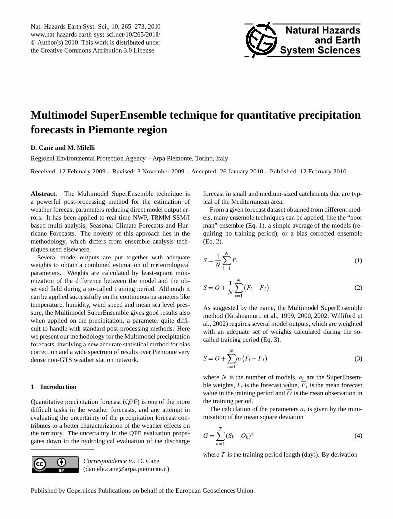
Arpa Piemonte manages a wide non-GTS weather stationnetwork. For this work, we used the data collected in the pe-riod March 2006–August 2008 from 342 stations. The datawere averaged over the 13 warning areas designed by ARPAPiemonte in collaboration with the Civil Protection Depart-ment (Fig. 2) on a 6-h basis up to +72 h and for each of themthe maximum values of observed precipitation has been as-signed. Each warning areas so identified contains on average26 stations, with a minimum of 11 and a maximum of 39.The chosen spatial scale is practical for the use in an alertsystem in medium- and large-scale catchments, but it is toomuch coarse for the discharge calculations in the smallestcatchments. Finer resolution calculation are still under in-vestigation.

The models used in this research work are the ECMWFIFS global model (resolution: 0.25◦) and the 0.0625◦

resolution limited area models of the COSMO Consor-tium covering North-Wester Italy: COSMO-I7 (developedby USAM, ARPA-SIM, ARPA Piemonte), COSMO-EU(Deutscher Wetterdienst) and COSMO-7 (MeteoSwiss). Ithas to be highlighted that our operational implementation(see Sect. 4.3) is based on the forecasts given by the ECMWFmodel and by the Italian COSMO model only (seewww.cosmo-model.orgfor a more comprehensive overview of theConsortium activities and developments). The model fore-casts are assigned to the same warning areas by taking theaverage and maximum values of the gridpoints falling intothe given area. (ECMWF model:∼5 points/warning area;COSMO models:∼56 points/warning area)

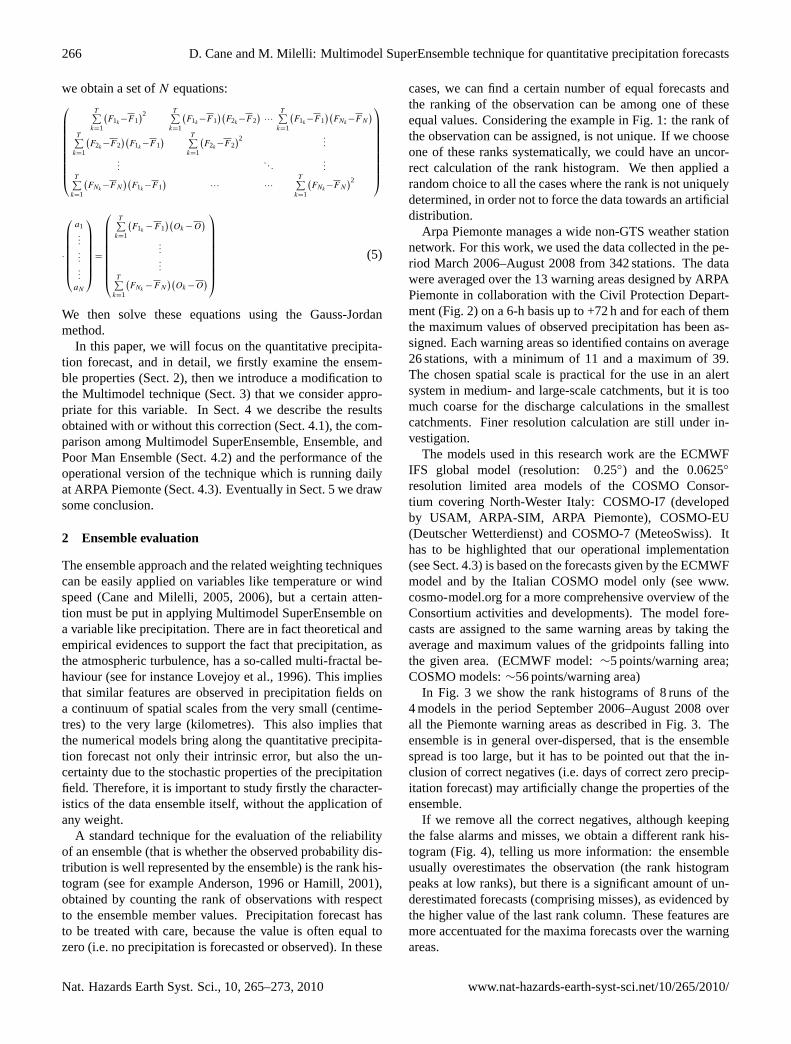
In Fig. 3 we show the rank histograms of 8 runs of the4 models in the period September 2006–August 2008 overall the Piemonte warning areas as described in Fig. 3. Theensemble is in general over-dispersed, that is the ensemblespread is too large, but it has to be pointed out that the in-clusion of correct negatives (i.e. days of correct zero precip-itation forecast) may artificially change the properties of theensemble.

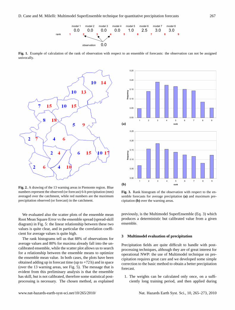
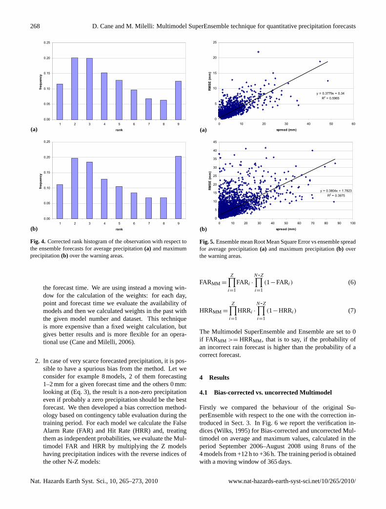
If we remove all the correct negatives, although keepingthe false alarms and misses, we obtain a different rank his-togram (Fig. 4), telling us more information: the ensembleusually overestimates the observation (the rank histogrampeaks at low ranks), but there is a significant amount of un-derestimated forecasts (comprising misses), as evidenced bythe higher value of the last rank column. These features aremore accentuated for the maxima forecasts over the warningareas.

Nat. Hazards Earth Syst. Sci., 10, 265–273, 2010 www.nat-hazards-earth-syst-sci.net/10/265/2010/

www.cosmo-model.org

www.cosmo-model.org

D. Cane and M. Milelli: Multimodel SuperEnsemble technique for quantitative precipitation forecasts 267

10

model 1 model 2 model 3 model 4 model 5 model 6 model 7 model 8

0.0 0.0 0.0 0.0 1.0 2.5 3.0 3.0rank 1 2 3 4 5 6 7 8 9

observation 0.0

Figure 1. Example of calculation of the rank of observation with respect to an ensemble of

forecasts: the observation can not be assigned univocally.

Figure 2. A drawing of the 13 warning areas in Piemonte region. Blue numbers represent the

observed (or forecast) 6-hours precipitation (mm) averaged over the catchment, while red

numbers are the maximum precipitation observed (or forecast) in the catchment.

Fig. 1. Example of calculation of the rank of observation with respect to an ensemble of forecasts: the observation can not be assignedunivocally.

10

model 1 model 2 model 3 model 4 model 5 model 6 model 7 model 8

0.0 0.0 0.0 0.0 1.0 2.5 3.0 3.0rank 1 2 3 4 5 6 7 8 9

observation 0.0

Figure 1. Example of calculation of the rank of observation with respect to an ensemble of

forecasts: the observation can not be assigned univocally.

Figure 2. A drawing of the 13 warning areas in Piemonte region. Blue numbers represent the

observed (or forecast) 6-hours precipitation (mm) averaged over the catchment, while red

numbers are the maximum precipitation observed (or forecast) in the catchment.

Fig. 2. A drawing of the 13 warning areas in Piemonte region. Bluenumbers represent the observed (or forecast) 6-h precipitation (mm)averaged over the catchment, while red numbers are the maximumprecipitation observed (or forecast) in the catchment.

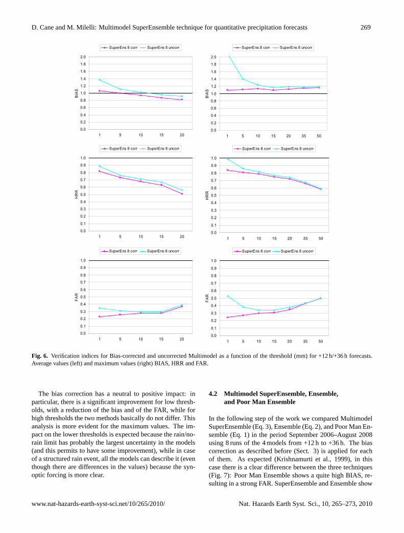
We evaluated also the scatter plots of the ensemble meanRoot Mean Square Error vs the ensemble spread (spread-skilldiagram) in Fig. 5: the linear relationship between these twovalues is quite clear, and in particular the correlation coeffi-cient for average values is quite high.

The rank histograms tell us that 88% of observations foraverage values and 80% for maxima already fall into the un-calibrated ensemble, while the scatter plot allows us to searchfor a relationship between the ensemble means to optimizethe ensemble mean value. In both cases, the plots have beenobtained adding up in forecast time (up to +72 h) and in space(over the 13 warning areas, see Fig. 5). The message that isevident from this preliminary analysis is that the ensemblehas skill, but is not calibrated, therefore some statistical post-processing is necessary. The chosen method, as explained

(a)

11

a)

0.00

0.05

0.10

0.15

0.20

0.25

1 2 3 4 5 6 7 8 9

rank

freq

uenc

y

b)

0.00

0.05

0.10

0.15

0.20

0.25

1 2 3 4 5 6 7 8 9

rank

freq

uenc

y

Figure 3: Rank histogram of the observation with respect to the ensemble forecasts for

average precipitation (a) and maximum precipitation (b) over the warning areas.

(b)

11

a)

0.00

0.05

0.10

0.15

0.20

0.25

1 2 3 4 5 6 7 8 9

rank

freq

uenc

y

b)

0.00

0.05

0.10

0.15

0.20

0.25

1 2 3 4 5 6 7 8 9

rank

freq

uenc

y

Figure 3: Rank histogram of the observation with respect to the ensemble forecasts for

average precipitation (a) and maximum precipitation (b) over the warning areas.

Fig. 3. Rank histogram of the observation with respect to the en-semble forecasts for average precipitation(a) and maximum pre-cipitation(b) over the warning areas.

previously, is the Multimodel SuperEnsemble (Eq. 3) whichproduces a deterministic but calibrated value from a givenensemble.

3 Multimodel evaluation of precipitation

Precipitation fields are quite difficult to handle with post-processing techniques, although they are of great interest foroperational NWP: the use of Multimodel technique on pre-cipitation requires great care and we developed some simplecorrection to the basic method to obtain a better precipitationforecast.

1. The weights can be calculated only once, on a suffi-ciently long training period, and then applied during

www.nat-hazards-earth-syst-sci.net/10/265/2010/ Nat. Hazards Earth Syst. Sci., 10, 265–273, 2010


(a)

12

a)

0.00

0.05

0.10

0.15

0.20

0.25

1 2 3 4 5 6 7 8 9

rank

freq

uenc

y

b)

0.00

0.05

0.10

0.15

0.20

0.25

1 2 3 4 5 6 7 8 9

rank

frequ

ency

Figure 4: Corrected rank histogram of the observation with respect to the ensemble forecasts

for average precipitation (a) and maximum precipitation (b) over the warning areas.

(b)

12

a)

0.00

0.05

0.10

0.15

0.20

0.25

1 2 3 4 5 6 7 8 9

rank

freq

uenc

y

b)

0.00

0.05

0.10

0.15

0.20

0.25

1 2 3 4 5 6 7 8 9

rank

frequ

ency

Figure 4: Corrected rank histogram of the observation with respect to the ensemble forecasts

for average precipitation (a) and maximum precipitation (b) over the warning areas.

Fig. 4. Corrected rank histogram of the observation with respect tothe ensemble forecasts for average precipitation(a) and maximumprecipitation(b) over the warning areas.

the forecast time. We are using instead a moving win-dow for the calculation of the weights: for each day,point and forecast time we evaluate the availability ofmodels and then we calculated weights in the past withthe given model number and dataset. This techniqueis more expensive than a fixed weight calculation, butgives better results and is more flexible for an opera-tional use (Cane and Milelli, 2006).

2. In case of very scarce forecasted precipitation, it is pos-sible to have a spurious bias from the method. Let weconsider for example 8 models, 2 of them forecasting1–2 mm for a given forecast time and the others 0 mm:looking at (Eq. 3), the result is a non-zero precipitationeven if probably a zero precipitation should be the bestforecast. We then developed a bias correction method-ology based on contingency table evaluation during thetraining period. For each model we calculate the FalseAlarm Rate (FAR) and Hit Rate (HRR) and, treatingthem as independent probabilities, we evaluate the Mul-timodel FAR and HRR by multiplying the Z modelshaving precipitation indices with the reverse indices ofthe other N-Z models:

(a)

13

a)

y = 0.3779x + 0.34R2 = 0.5965

0

5

10

15

20

25

0 10 20 30 40 50 60

spread (mm)

RMSE

(mm

)

b)

y = 0.3804x + 1.7823R2 = 0.3975

0

5

10

15

20

25

30

35

40

45

0 10 20 30 40 50 60 70 80 90 100

spread (mm)

RMSE

(mm

)

Figure 5: Ensemble mean Root Mean Square Error vs ensemble spread for average

precipitation (a) and maximum precipitation (b) over the warning areas.

(b)

13

a)

y = 0.3779x + 0.34R2 = 0.5965

0

5

10

15

20

25

0 10 20 30 40 50 60

spread (mm)

RMSE

(mm

)

b)

y = 0.3804x + 1.7823R2 = 0.3975

0

5

10

15

20

25

30

35

40

45

0 10 20 30 40 50 60 70 80 90 100

spread (mm)

RMSE

(mm

)

Figure 5: Ensemble mean Root Mean Square Error vs ensemble spread for average

precipitation (a) and maximum precipitation (b) over the warning areas.

Fig. 5. Ensemble mean Root Mean Square Error vs ensemble spreadfor average precipitation(a) and maximum precipitation(b) overthe warning areas.

FARMM =

Z∏i=1

FARi ·

N-Z∏i=1

(1−FARi) (6)

HRRMM =

Z∏i=1

HRRi ·

N-Z∏i=1

(1−HRRi) (7)

The Multimodel SuperEnsemble and Ensemble are set to 0if FARMM >= HRRMM , that is to say, if the probability ofan incorrect rain forecast is higher than the probability of acorrect forecast.

4 Results

4.1 Bias-corrected vs. uncorrected Multimodel

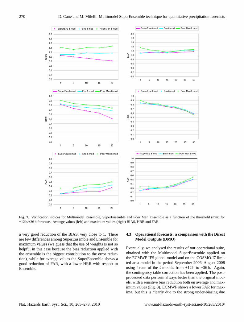
Firstly we compared the behaviour of the original Su-perEnsemble with respect to the one with the correction in-troduced in Sect. 3. In Fig. 6 we report the verification in-dices (Wilks, 1995) for Bias-corrected and uncorrected Mul-timodel on average and maximum values, calculated in theperiod September 2006–August 2008 using 8 runs of the4 models from +12 h to +36 h. The training period is obtainedwith a moving window of 365 days.



0.0

0.2

0.4

0.6

0.8

1.0

1.2

1.4

1.6

1.8

2.0

1 5 10 15 20

BIA

S

SuperEns 8 corr SuperEns 8 uncorr

0.0

0.2

0.4

0.6

0.8

1.0

1.2

1.4

1.6

1.8

2.0

1 5 10 15 20 35 50

BIA

S


0.0

0.1

0.2

0.3

0.4

0.5

0.6

0.7

0.8

0.9

1.0

1 5 10 15 20

HR

R


0.0

0.1

0.2

0.3

0.4

0.5

0.6

0.7

0.8

0.9

1.0

1 5 10 15 20 35 50

HR

R


0.0

0.1

0.2

0.3

0.4

0.5

0.6

0.7

0.8

0.9

1.0

1 5 10 15 20

FAR


0.0

0.1

0.2

0.3

0.4

0.5

0.6

0.7

0.8

0.9

1.0

1 5 10 15 20 35 50

FAR


Fig. 6. Verification indices for Bias-corrected and uncorrected Multimodel as a function of the threshold (mm) for +12 h/+36 h forecasts.Average values (left) and maximum values (right) BIAS, HRR and FAR.

The bias correction has a neutral to positive impact: inparticular, there is a significant improvement for low thresh-olds, with a reduction of the bias and of the FAR, while forhigh thresholds the two methods basically do not differ. Thisanalysis is more evident for the maximum values. The im-pact on the lower thresholds is expected because the rain/no-rain limit has probably the largest uncertainty in the models(and this permits to have some improvement), while in caseof a structured rain event, all the models can describe it (eventhough there are differences in the values) because the syn-optic forcing is more clear.

4.2 Multimodel SuperEnsemble, Ensemble,and Poor Man Ensemble

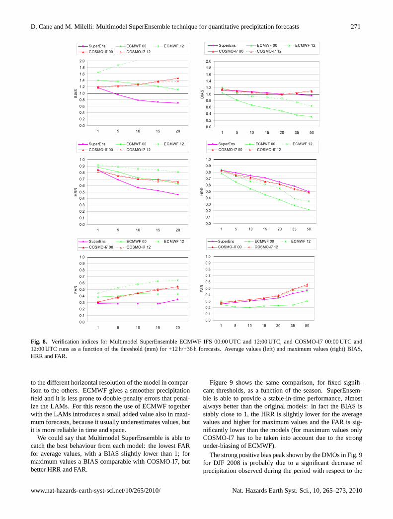
In the following step of the work we compared MultimodelSuperEnsemble (Eq. 3), Ensemble (Eq. 2), and Poor Man En-semble (Eq. 1) in the period September 2006–August 2008using 8 runs of the 4 models from +12 h to +36 h. The biascorrection as described before (Sect. 3) is applied for eachof them. As expected (Krishnamurti et al., 1999), in thiscase there is a clear difference between the three techniques(Fig. 7): Poor Man Ensemble shows a quite high BIAS, re-sulting in a strong FAR. SuperEnsemble and Ensemble show



0.0

0.2

0.4

0.6

0.8

1.0

1.2

1.4

1.6

1.8

2.0

1 5 10 15 20

BIA

S

SuperEns 8 mod Ens 8 mod Poor Man 8 mod

0.0

0.2

0.4

0.6

0.8

1.0

1.2

1.4

1.6

1.8

2.0

1 5 10 15 20 35 50

BIA

S


0.0

0.1

0.2

0.3

0.4

0.5

0.6

0.7

0.8

0.9

1.0

1 5 10 15 20

HR

R


0.0

0.1

0.2

0.3

0.4

0.5

0.6

0.7

0.8

0.9

1.0

1 5 10 15 20 35 50

HR

R


0.0

0.1

0.2

0.3

0.4

0.5

0.6

0.7

0.8

0.9

1.0

1 5 10 15 20

FAR


0.0

0.1

0.2

0.3

0.4

0.5

0.6

0.7

0.8

0.9

1.0

1 5 10 15 20 35 50

FAR


Fig. 7. Verification indices for Multimodel Ensemble, SuperEnsemble and Poor Man Ensemble as a function of the threshold (mm) for+12 h/+36 h forecasts. Average values (left) and maximum values (right) BIAS, HRR and FAR.

a very good reduction of the BIAS, very close to 1. Thereare few differences among SuperEnsemble and Ensemble formaximum values (we guess that the use of weights is not sohelpful in this case because the bias reduction applied withthe ensemble is the biggest contribution to the error reduc-tion), while for average values the SuperEnsemble shows agood reduction of FAR, with a lower HRR with respect toEnsemble.

4.3 Operational forecasts: a comparison with the DirectModel Outputs (DMO)

Eventually, we analysed the results of our operational suite,obtained with the Multimodel SuperEnsemble applied onthe ECMWF IFS global model and on the COSMO-I7 limi-ted area model in the period September 2006–August 2008using 4 runs of the 2 models from +12 h to +36 h. Again,the contingency table correction has been applied. The post-processed data perform always better than the original mod-els, with a sensitive bias reduction both on average and max-imum values (Fig. 8). ECMWF shows a lower FAR for max-ima, but this is clearly due to the strong under-biasing due



0.0

0.2

0.40.6

0.8

1.0

1.2

1.41.6

1.8

2.0

1 5 10 15 20

BIA

S

SuperEns ECMWF 00 ECMWF 12COSMO-I7 00 COSMO-I7 12

0.0

0.2

0.4

0.6

0.81.0

1.2

1.4

1.6

1.8

2.0

1 5 10 15 20 35 50

BIA

S


0.0

0.1

0.2

0.3

0.40.5

0.6

0.7

0.8

0.9

1.0

1 5 10 15 20

HR

R


0.0

0.1

0.2

0.3

0.4

0.5

0.6

0.7

0.8

0.9

1.0

1 5 10 15 20 35 50

HR

R


0.0

0.1

0.2

0.3

0.4

0.5

0.6

0.7

0.8

0.9

1.0

1 5 10 15 20

FAR


0.0

0.1

0.2

0.3

0.4

0.5

0.6

0.7

0.8

0.9

1.0

1 5 10 15 20 35 50

FAR


FIG. 8 Fig. 8. Verification indices for Multimodel SuperEnsemble ECMWF IFS 00:00 UTC and 12:00 UTC, and COSMO-I7 00:00 UTC and

12:00 UTC runs as a function of the threshold (mm) for +12 h/+36 h forecasts. Average values (left) and maximum values (right) BIAS,HRR and FAR.

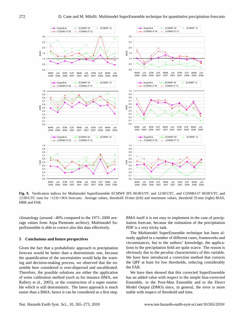
to the different horizontal resolution of the model in compar-ison to the others. ECMWF gives a smoother precipitationfield and it is less prone to double-penalty errors that penal-ize the LAMs. For this reason the use of ECMWF togetherwith the LAMs introduces a small added value also in maxi-mum forecasts, because it usually underestimates values, butit is more reliable in time and space.

We could say that Multimodel SuperEnsemble is able tocatch the best behaviour from each model: the lowest FARfor average values, with a BIAS slightly lower than 1; formaximum values a BIAS comparable with COSMO-I7, butbetter HRR and FAR.

Figure 9 shows the same comparison, for fixed signifi-cant thresholds, as a function of the season. SuperEnsem-ble is able to provide a stable-in-time performance, almostalways better than the original models: in fact the BIAS isstably close to 1, the HRR is slightly lower for the averagevalues and higher for maximum values and the FAR is sig-nificantly lower than the models (for maximum values onlyCOSMO-I7 has to be taken into account due to the strongunder-biasing of ECMWF).

The strong positive bias peak shown by the DMOs in Fig. 9for DJF 2008 is probably due to a significant decrease ofprecipitation observed during the period with respect to the



0.0

0.5

1.0

1.5

2.0

2.5

3.0

MAM2006

JJA2006

SON2006

DJF2007

MAM2007

JJA2007

SON2007

DJF2008

MAM2008

JJA2008

BIA

S


0.0

0.5

1.0

1.5

2.0

2.5

3.0

MAM2006

JJA2006

SON2006

DJF2007

MAM2007

JJA2007

SON2007

DJF2008

MAM2008

JJA2008

BIA

S


0.00.10.20.30.40.50.60.70.80.91.0

MAM2006

JJA2006

SON2006

DJF2007

MAM2007

JJA2007

SON2007

DJF2008

MAM2008

JJA2008

HR

R


0.00.10.20.30.40.50.60.70.80.91.0

MAM2006

JJA2006

SON2006

DJF2007

MAM2007

JJA2007

SON2007

DJF2008

MAM2008

JJA2008

HR

R


0.00.10.20.30.40.50.60.70.80.91.0

MAM2006

JJA2006

SON2006

DJF2007

MAM2007

JJA2007

SON2007

DJF2008

MAM2008

JJA2008

FAR


0.00.10.20.30.40.50.60.70.80.91.0

MAM2006

JJA2006

SON2006

DJF2007

MAM2007

JJA2007

SON2007

DJF2008

MAM2008

JJA2008

FAR


Fig. 9. Verification indices for Multimodel SuperEnsemble ECMWF IFS 00:00 UTC and 12:00 UTC, and COSMO-I7 00:00 UTC and12:00 UTC runs for +12 h/+36 h forecasts. Average values, threshold 10 mm (left) and maximum values, threshold 35 mm (right) BIAS,HRR and FAR.

climatology (around –40% compared to the 1971–2000 ave-rage values from Arpa Piemonte archive); Multimodel Su-perEnsemble is able to correct also this data effectively.

5 Conclusions and future perspectives

Given the fact that a probabilistic approach to precipitationforecast would be better than a deterministic one, becausethe quantification of the uncertainties would help the warn-ing and decision-making process, we observed that the en-semble here considered is over-dispersed and uncalibrated.Therefore, the possible solutions are either the applicationof some calibration method (such as for instance BMA, seeRaftery et al., 2005), or the construction of a super ensem-ble which is still deterministic. The latest approach is mucheasier than a BMA, hence it can be considered as a first step.

BMA itself it is not easy to implement in the case of precip-itation forecast, because the estimation of the precipitationPDF is a very tricky task.

The Multimodel SuperEnsemble technique has been al-ready applied in a number of different cases, frameworks andcircumstances, but to the authors’ knowledge, the applica-tions to the precipitation field are quite scarce. The reason isobviously due to the peculiar characteristics of this variable.We have here introduced a correction method that correctsthe QPF at least for low thresholds, reducing considerablythe FAR.

We have then showed that this corrected SuperEnsemblehas an added value with respect to the simple bias-correctedEnsemble, to the Poor-Man Ensemble and to the DirectModel Output (DMO) since, in general, the error is morestable with respect of threshold and time.



We are now working on Multimodel SuperEnsemble errorevaluation methods, including bootstrap, and on ensemblecalibration methods, in order to keep a probabilistic point ofview. We are trying to evaluate the correct PDF of the Multi-model forecasts starting from the observed PDF conditionedto the forecasts, combining Multimodel SuperEnsemble anda BMA-like ensemble dressing: the first results are encour-aging and we are planning to apply the so-found probabilisticprecipitation forecasts as the input of our hydrologic chain,in order to evaluate the uncertainties in the discharge calcu-lations. The use of finer spatial resolution (for example: atstation locations) will be necessary for this application.

Moreover we are working on the downscaling of RegionalClimatic Models with a Multimodel SuperEnsemble tech-nique: in this case we use as training period the control runsand we apply the weights calculated in this period to themodel scenarios.

Acknowledgements.This work is supported by the ItalianCivil Protection Department. We wish to thank our colleaguesElena Oberto and Marco Turco for the useful discussions about theprecipitation bias correction and Renata Pelosini for her support.

Edited by: S. Michaelides, K. Savvidou, and F. TymviosReviewed by: two anonymous referees

References

Anderson, J. L.: A method for producing and evaluating probabilis-tic forecasts from ensemble model integrations, J. Climate, 9,1518–1530, 1996.

Cane, D. and Milelli, M.: Use of Multimodel SuperEnsemble Tech-nique for Mountain-area weather forecast in the Olympic Areaof Torino 2006, Croat. Met. J., 40, 215–219, 2005.

Cane, D. and Milelli, M.: Weather forecasts with Multimodel Su-perEnsemble Technique in a complex orography region, Meteo-rol. Z., 15(2), 1–8, 2006.

Hamill, T. M.: Interpretation of rank histograms for verifying en-semble forecasts, Mon. Weather Rev., 129, 550–560, 2001.

Krishnamurti, T. N., Kishtawal, C. M., Larow, T. E., Bachiochi, D.R., Zhang, Z., Williford, C. E., Gadgil, S., and Surendran, S.: Im-proved weather and seasonal climate forecasts from MultimodelSuperensemble, Science, 285, 1548–1550, 1999.

Krishnamurti, T. N., Kishtawal, C. M., Larow, T. E., Bachiochi, D.R., Zhang, Z., Williford, C. E., Gadgil, S., and Surendran, S.:Multi-model superensemble forecasts for weather and seasonalclimate, J. Climate, 13, 4217–4227, 2000.

Krishnamurti, T. N., Stefanova, L., Chakraborty, A., Vijaya Ku-mar, T. S. V., Cocke, S., Bachiochi, D. R., and Mackey, B.: Sea-sonal Forecasts of precipitation anomalies for North Americanand Asian Monsoons, J. Meteorol. Soc. Jpn, 80(6), 1415–1426,2002.

Lovejoy, S., Duncan, M. R., and Schertzer, D.: Scalar multi-fractalradar observer’s problem, J. Geophys. Res.-Atmos., 101(D21),26479–26491, 1996.

Raftery, A. E., Gneiting, T., Balabdaoui, F., and Polakowski, M.:Using a Bayesian model averaging to calibrate forecast ensem-bles, Mon. Weather Rev., 133, 1155–1174, 2005.

Wilks, D. S.: Statistical Methods in the Atmospheric Sciences. AnIntroduction, Academic Press, San Diego, 467 pp., 1995.

Williford, C. E., Krishnamurti, T. N., Correa-Torres, R. J., Cocke,S., Christidis, Z., and Vijaya Kumar, T. S. V.: Real Time Mul-tianalysis/Multimodel Superensemble Forecasts of Precipitationusing TRMM and SSM/I Products, Mon. Weather Rev., 131/8,1878–1894, 2002.


Documents

Multimodel SuperEnsemble technique for quantitative ...D. Cane and M. Milelli: Multimodel SuperEnsemble technique for quantitative precipitation forecasts 267 10 model 1 model 2 model